Identifying Temporal Change in Urban Water Bodies Using OpenStreetMap and Landsat Imagery: A Study of Hangzhou City

Abstract

As one of the most important ecosystems, the water body is losing water during the rapid development of the city. To understand the impacts on water body change during the rapid urbanization period, this study combines data from the OpenStreetMap platform with Landsat 5/Thematic Mapper images to effectively and accurately identify small urban water bodies. The findings indicate that the trained U-net convolutional neural network (U-Net) water body extraction model and loss function combining Focal Loss and Dice Loss adopted in this study demonstrate high precision in identifying water bodies within the main urban area of Hangzhou, with an accuracy rate of 94.3%. Trends of decrease in water areas with a continuous increase in landscape fragmentation, particularly for the plain river network, were observed from 1985 to 2010, indicating a weaker connection between water bodies resulting from rapid urbanization. Large patches of water bodies, such as natural lakes and big rivers, located at divisions at the edge of the city are susceptible to disappearing during the rapid outward expansion. However, due to the limitations and strict control of development, water bodies, referring to as wetland, slender canals, and plain river networks, in the traditional center division of the city, are preserved well. Combined with the random forest classification method and the U-Net water body extraction model, land use changes from 1985 to 2010 are calculated. Reclamation along the Qiantang River accounts for the largest conversion area between water bodies and cultivated land, constituting more than 90% of the total land use change area, followed by the conversion of water bodies into construction land, particularly in the northeast of Xixi Wetland. Notably, the conversion of various land use types within Xixi Wetland into construction land plays a significant role in the rise of the carbon footprint.

1. Introduction

Urban water bodies, including rivers, springs, lakes, streams, reservoirs, and ponds, are crucial components of natural and man-made aquatic ecosystems. They serve as vital resources for preserving public health, sustaining both human productivity and urban ecology, and protecting the quality of urban environments [1,2,3]. Accurately capturing the evolving characteristics of urban water bodies is crucial for ensuring the sufficiency of available water resources, regulating the regional climate, and mitigating the heat island effect in cities [4].

However, traditional field methods used to analyze urban water bodies, such as field sampling for the analysis of water quality, underwater sediment analysis, meteorological observations, and biodiversity surveys, are time-consuming and labor-intensive. In contrast, rapid advances in satellite remote sensing (RS) [5,6,7] technology have enabled efficient qualitative and quantitative monitoring of urban water bodies over large areas [8,9]. In recent years, RS with high-resolution satellites has greatly contributed to fine-scale ground observation. The Landsat series of satellites, first launched in 1972 by the United States, has consistently provided earth observation images with relatively high spatial resolution. This is particularly useful for long-term observation through the recovery and reconstruction of historical satellite data with high precision, especially in the study of land use change and related trends. Furthermore, the 30 m resolution of Landsat imagery is adequate for observing most surface water resources, especially medium-large water bodies, even those that are intricately shaped, such as linear, circular, and irregularly distributed water bodies [10,11,12,13]. However, with the improving requirements of observation, the identification and extraction of small water bodies using satellite images with a ground resolution of 30 m or so need to be further improved in terms of accuracy and efficiency. Moreover, the traditional water body extraction methods based on satellite RS technology have defects in determining the threshold for water body identification and have low levels of precision and a low degree of automation [14,15,16].

In recent years, the development of computing hardware and related technology has led to significant advancements in computing power, enabling rapid progress in the field of machine learning. Prominent machine learning methods, such as maximum likelihood estimation [17], support vector machine (SVM) [18], and random forest (RF) [19], have been extensively applied in image classification, quantitative RS inversion, and water body extraction [20,21]. However, it should be noted that machine learning relies on artificial feature extraction and requires a substantial number of samples to train the classifier. The quality of these samples directly affects the accuracy of water body extraction. Obtaining a sufficient quantity of high-quality training samples for large-scale water bodies can be challenging [22,23], thus hindering machine learning in the recognition of ground objects based on satellite RS images. Deep learning, specifically convolutional neural networks, has emerged as a powerful tool in satellite image processing [8,24,25]. It offers potential solutions for object extraction, image segmentation, and image classification, among others [26,27].

The present study takes the city of Hangzhou in Zhejiang, China, as a study area to establish methods to accurately identify the changes in water body areas in cities with rapid urbanization, to illustrate how urbanization changes the water body, including area and landscape fragmentation, and to reveal the potential effect of changes in water bodies on regional carbon sinks and sources. The study is designed with the following three goals: (1) to propose an applicable deep learning algorithm and procedure that has good performance in extracting small and/or slender water bodies and other land use types with acceptable accuracy from Landsat5/Thematic Mapper (TM) imagery; (2) to identify the main factor affecting the interannual changes in the area, patches, and landscape fragmentation of water bodies within the main urban area of Hangzhou from 1986–2010, a period of rapid urbanization; and (3) to analyze the carbon footprint when water body areas were changed into other land use types, including cultivated land, woodland, grassland, construction land, and unused land in Hangzhou. The study aims to be beneficial to the urban management and protection of water resources during rapid urbanization and provide a method that can be used to accurately estimate carbon sinks and sources.

2. Research Area and Data Acquisition

2.1. Study Area

This study focuses on the water bodies within the main urban area of the city of Hangzhou. Hangzhou, the capital of Zhejiang Province, is situated in the alluvial plain of the Yangtze River Delta in eastern China and is geographically positioned between 29°11′–30°33′N and 118°21′–120°30′E. The city features an intricate network of slender rivers and a variety of lakes, ponds, springs, and reservoirs of various sizes and shapes, forming an extensive plain water system spanning in all directions and accounting for approximately 8% of the city’s total area. As a historically significant city renowned for its rich water culture, Hangzhou has notable water bodies, including the oldest canal system in China, the picturesque West Lake, and Xixi Wetland Reserve [28,29]. In addition, the Qiantang River flows around the city in the northeast and connects with the trumpet-shaped Hangzhou Bay. With the world-famous QianTang Tide, saline water intrusion has endangered the safety and quality of drinking water for a long time. Hangzhou has expanded rapidly in recent decades, resulting in significant changes in land use patterns. The increasing demand for land has led to a reduction in the water area, thereby greatly affecting the distribution characteristics of surface water [30,31,32]. A map of eastern China and the latest administrative division map of Hangzhou are shown in Figure 1.

2.2. Research Data

2.2.1. Satellite Data

This study used the Landsat series satellite imagery to derive the spatial and temporal distribution of water bodies and land use pattern change in the study area. The satellite images were selected based on the following criteria: (1) A time series of images was visually selected when significant changes in water bodies occurred. The period of 1985–2010 was selected because more frequent and dramatic changes in water area and patches occurred at this time when compared with the periods before 1985 and after 2010. (2) Using the satellite images with the same sensor, the imaging time of Landsat 5 ranged from 1984 to 2013, which effectively covered the period of this study and ensured the consistency of satellite data and quality. (3) With the goal of using satellite images with good quality, only images with less than 10% cloud cover were used. (4) To avoid the influence of water level changes caused by weather, only satellite images acquired in the dry season were selected whenever possible. Detailed information about the selected images is shown in Table 1. Landsat5/TM images with column 119 and row 39 were downloaded from the Geospatial Data Cloud (https://www.gscloud.cn).

2.2.2. OpenStreetMap Data

OpenStreetMap (OSM) is a non-commercial platform (www.openstreetmap.org) that is spontaneously provided and maintained by hobbyists worldwide. It offers a wide range of data, including data about highways, railways, water bodies, buildings, and administrative borders [33]. The OSM website is freely available and allows users to set up their own servers and modify data with detailed and updated geographic information worldwide. However, the reliability and quality of the data on the OSM platform are affected by the expertise of its users, the accuracy of data acquisition equipment, and inconsistencies in data sources [34,35]. The present study used OSM data to create data labels that align with Landsat 5 and TM images. The OSM drainage data, which includes high-precision information on topological relationships and essential related attributes such as latitude, longitude, and other relevant spatial details, was used to correct the satellite images.

Table 1. Information on selected Landsat 5/Thematic Mapper (TM) satellite images.

Year	Data	Cloud Cover	Number
1985	11 January	1.56%	LT51190391985011HAJ00
1986	03 March	0%	LT51190391986062HAJ00
1988	05 December	0%	LT51190391988340HAJ00
1990	08 October	0%	LT51190391990281HAJ00
1992	15 January	1%	LT51190391992015BJC0
1994	12 May	0%	LT51190391994132XXX02
1995	09 December	0%	LT51190391995343CLT00
1996	11 December	0%	LT51190391996346CLT00
1998	17 December	0%	LT51190391998351HAJ00
2000	17 September	0%	LT51190392000261BJC00
2002	11 February	0%	LT51190392002042BJC00
2004	14 October	0%	LT51190392004288BJC00
2005	17 October	0.18%	LT51190392005290BJC02
2006	29 May	4.4%	LT51190392006149BJC00
2008	28 February	0%	LT51190392008059BJC00
2010	18 December	7%	LT51190392010352BJC00

Table 1. Information on selected Landsat 5/Thematic Mapper (TM) satellite images.

Year	Data	Cloud Cover	Number
1985	11 January	1.56%	LT51190391985011HAJ00
1986	03 March	0%	LT51190391986062HAJ00
1988	05 December	0%	LT51190391988340HAJ00
1990	08 October	0%	LT51190391990281HAJ00
1992	15 January	1%	LT51190391992015BJC0
1994	12 May	0%	LT51190391994132XXX02
1995	09 December	0%	LT51190391995343CLT00
1996	11 December	0%	LT51190391996346CLT00
1998	17 December	0%	LT51190391998351HAJ00
2000	17 September	0%	LT51190392000261BJC00
2002	11 February	0%	LT51190392002042BJC00
2004	14 October	0%	LT51190392004288BJC00
2005	17 October	0.18%	LT51190392005290BJC02
2006	29 May	4.4%	LT51190392006149BJC00
2008	28 February	0%	LT51190392008059BJC00
2010	18 December	7%	LT51190392010352BJC00

3. Methodology

Figure 2 illustrates the fundamental technical workflow of this study. First, the selected Landsat5/TM images from 1985–2010 and OSM data were pre-processed to generate a dataset of water bodies for training the U-net convolutional neural network (U-Net) deep learning model. The proposed method underwent a series of accuracy evaluations and model optimizations. Second, the trained U-Net model was compared with traditional water body extraction models, including the modified normalized difference water index (MNDWI), automated water body extraction index (AWEI), and SVM. The advantages of U-Net deep learning technology in this context were assessed. Third, the trained U-Net model was used to extract water bodies from the main urban area of Hangzhou from 1986 to 2010, enabling a comprehensive analysis of interannual changes in area, patch number, and landscape fragmentation. The main stimulation inducing the changes in the water area was identified. Meanwhile, the RF method was employed to classify land use within the main urban area of Hangzhou, facilitating an assessment of variations in carbon footprint under rapid urbanization over a distinct period.

3.1. Data Preprocessing

Before the satellite data were used for extracting water bodies and classifying different land use types, radiometric calibration, geometric correction, and atmospheric correction were performed with Environment for Visualizing Images (ENVI) software, Version 5.3 (Exelis VIS, Boulder, Colorado, CO, USA). It should be noted that atmospheric correction is particularly crucial to deriving accurate water information by mitigating the influence of the atmosphere. In the present study, the atmospheric correction tool in ENVI allows for precise correction and employed an elevation setting of 0.08 km, an urban aerosol model, and a 2-band aerosol inversion method. The latest administrative vector boundary data of the main urban area of Hangzhou (https://www.webmap.cn/commres.do?method=dataDownload, accessed on 30 April 2024) was used to crop the image to the study area.

To overcome inaccuracies in the data from the OSM platform, the OSM vector data for the water area in the main urban area of Hangzhou were adjusted to align with the actual Landsat 5/TM image using ArcGIS Version 10.8 software (Environmental Systems Research Institute, Redlands, CA, USA). This involves removing non-water areas, adding missing water areas, and modifying the vector data to accurately represent the actual water bodies.

3.2. Making Training Samples

The labeled data for water bodies consisted of binary raster data, comprising two parts: water bodies and non-water bodies. To obtain water body labeling data that aligned with the satellite images, the Landsat 5/TM images were cropped and resampled using ArcGIS. Values of 1 and 0 were assigned to water body regions and background regions, respectively (Figure 3).

The large number of parameters in the annotation dataset used in the present study could lead to memory overflow when these data are moved into the network. Moreover, a small sample size may not contain sufficient information about the water bodies, resulting in overfitting of the water body extraction model. Therefore, a large number of training samples and high complexity are required [36]. In the present study, data augmentation techniques such as rotation, flipping, and adding noise information were applied to the water body dataset, expanding the training dataset to approximately 2352 samples specifically for the water bodies in Hangzhou City. During model training, 60% of the samples were chosen as the training set, 20% as the validation set, and the remaining 20% as the test set.

3.3. Machine Learning

This study employed two machine-learning methods. Among them, U-Net based on the loss function optimization method is utilized to establish a water body extraction model, while RF is used to construct a land use type classification model.

3.3.1. U-Net

The U-Net deep learning model follows an “encoder-decoder” architecture. This experiment used the deep learning framework PyTorch, which provides a pre-trained U-Net network model.

The training process of the U-Net model is depicted in Figure 4. The original image samples and their corresponding samples are fed into the constructed network model. Through a series of upsampling and downsampling operations, the network generates predicted feature maps. Initially, the values in the convolution kernels are initialized with random numbers following a Gaussian distribution. These values are then gradually adjusted based on the previously mentioned loss function. The predicted feature maps are passed through a Softmax function to obtain the predicted probability distribution. The labeled samples are then compared with the predicted feature maps, and the loss value is calculated using the loss function. Through backpropagation, the model iteratively updates the parameters to minimize the loss value, resulting in a more accurate classification. Finally, the Adam optimizer is employed to update the parameters.

The loss function plays a crucial role in evaluating the disparity between the predicted and actual values produced by the model. A smaller loss function signifies the better performance of the model. Different loss functions can yield varying effects when used with different models.

During the training stage, the model takes the training data as input and produces predicted values through a series of calculations. By computing the differences between the predicted and actual values (represented as the loss value), the model updates the parameters within the network. As the training progresses, the predicted values generated by the model gradually approach the actual values, leading to improved learning outcomes.

3.3.2. Loss Function

The U-Net method generally adopts a pixel-based cross-entropy loss function. However, the incorrect identification of a water body with a small area may occur. To improve the recognition accuracy of small water bodies from the perspective of optimizing the loss function, a combination loss function combining Focal and Dice Losses was adopted in this study.

The Focal Loss is a kind of loss function that is used to solve model performance problems caused by a data imbalance in the image field. The definition formula for the two types of semantic segmentation is as follows:

$$\mathrm{FL}=\{\begin{array}{c}-\alpha {\left(1-p_n\right)}^r\log \left(p_n\right),r_n=1\\ -\left(1-\alpha \right){p_n}^r\log \left(1-p_n\right),r_n=0\end{array}$$

(1)

where p_n is the predicted value, and r_n is the true value of the sample. In addition, α is a balance factor, which is used to balance the unbalanced ratio of positive and negative samples, while γ is a parameter used to adjust the speed of the weight decline of a simple sample [37].

Dice Loss is a metric function used to evaluate the similarity between two samples; it ranges from 0 to 1. A higher value indicates greater similarity. Dice Loss operates on output and ground-truthed rasters, assessing the overlap between the two. For binary semantic segmentation tasks, the expression for Dice Loss can be given as:

$$\mathrm{DL}=1-\frac{{\sum }_{n=1}^N{p}_n{r}_n+\epsilon }{{\sum }_{n=1}^N{p}_n+r_n+\epsilon }-\frac{{\sum }_{n=1}^N(1-p_n)\left(1-r_n\right)+\epsilon }{{\sum }_{n=1}^{N}2-p_n-r_n+\epsilon }$$

(2)

where N is the total number of pixels, p_n is the predicted result, r_n is the true value of the sample, and ε is the adjustment parameter used to avoid the denominator being 0 [38].

The combination of Focal Loss and Dice Loss requires attention to scale both to the same order of magnitude, using −log to zoom in on Dice Loss and alpha to zoom out on Focal Loss.

3.3.3. Random Forest

The RF algorithm is a supervised classification method [39]. It uses the concept of ensemble learning by integrating multiple decision trees into a forest. Each decision tree within the forest independently classifies the input sample data, and the final classification is determined based on the majority vote from all the trees.

For the same batch of data samples, the same algorithm can only produce one tree. However, by repeatedly sampling a certain number of subsamples from the original dataset and creating new classifiers from each subsample, multiple classifiers can be obtained. The final output is determined by selecting the class with the highest number of votes among the classifiers.

3.4. Water Body Extraction Models and Accuracy Evaluation

3.4.1. Water Body Extraction Models

To verify the effect of water body extraction with U-Net, commonly used water body extraction methods, including MNDWI, AWEI, and SVM, were used to make the comparison.

An MNDWI is an improved normalized water body index [40] used to overcome the frequent noise of the normalized difference water index. An MNDWI has the advantage of distinguishing shadows from water bodies. The formula for MNDWI is as follows:

$$\mathrm{MNDWI}=\frac{\mathrm{Green}-\mathrm{MIR}}{\mathrm{Green}+\mathrm{MIR}}$$

(3)

where Green and MIR are the reflectance of green and mid-infrared bands of Landsat 5 and TM data, respectively.

An AWEI index has been proven to be conducive to eliminating urban shadows. The method is mainly divided into two types: AWEI_nsh and AWEI_sh, which are used when shadows are insignificant and significant, respectively. The formulas are as follows:

$${\mathrm{AWEI}}_{\mathrm{nsh}}=4\left(\mathrm{B}2-\mathrm{B}5\right)-\left(0.25\mathrm{B}4+2.75\mathrm{B}7\right)$$

(4)

$${\mathrm{AWEI}}_{\mathrm{sh}}=\mathrm{B}1+2.5\mathrm{B}2-1.5\left(\mathrm{B}4+\mathrm{B}5\right)-0.25\mathrm{B}7$$

(5)

where B1, B2, B4, B5, and B7 are values of bands 1, 2, 4, 5, and 7 of Landsat5/TM images, respectively.

An SVM is a supervised learning method that needs to manually select samples that can represent known categories and automatically classify images according to the information in these samples [41]. Sample selection is the key to high-precision water body extraction by an SVM. Water bodies and other land categories from the main urban area of Hangzhou were selected as training samples in this study. Totals of 200 water bodies and 500 non-water samples were manually selected, and then water bodies were extracted with an SVM.

3.4.2. Accuracy Evaluation

The classification results were divided into true positive (TP), false positive (FP), true negative (TN), and false negative (FN). The specific criteria are shown in

Table 2. Criteria for water body and non-water land classification results.

	True Value	Water	Non-Water
Predicted Value
Water body		True positive	False positive
Non-water body		False negative	True negative

.

Based on the four scenarios, this study selected the following five metrics to evaluate the accuracy of the water body extraction model: accuracy, precision, recall, F1 score, and mean intersection over union (mIoU) [19]. The calculation formulas for these metrics are as follows:

$$\mathrm{Accuracy}=\frac{\mathrm{TP}+\mathrm{TN}}{\mathrm{TP}+\mathrm{FN}+\mathrm{FP}+\mathrm{TN}}$$

(6)

$$\mathrm{Precision}=\frac{\mathrm{TP}}{\mathrm{TP}+\mathrm{FP}}$$

(7)

$$\mathrm{Recall}=\frac{\mathrm{TP}}{\mathrm{TP}+\mathrm{FN}}$$

(8)

$$F1=2\times \frac{\mathrm{Precision}\times \mathrm{Recall}}{\mathrm{Precision}+\mathrm{Recall}}$$

(9)

$$\mathrm{mIoU}=\frac{\mathrm{TP}}{\mathrm{FP}+\mathrm{FN}+\mathrm{TP}}$$

(10)

3.5. Land Use Types and Carbon Footprint Estimation

Based on the national standard of the People’s Republic of China, “Classification of Land Use Status” [42], the present study divided the transformation of water body area into five types: construction land, cultivated land, woodland, grassland, and unused land. The carbon footprint is the difference between carbon emission (carbon source) and carbon uptake (carbon sink). The carbon footprint of cultivated land, woodland, grassland, water area, and unused land was directly calculated using a fixed carbon footprint coefficient. The calculation formula is as follows:

$$C_i={\displaystyle \sum }{A}_i\times a_i$$

(11)

where C_i is the carbon footprint, A_i is the area of a certain type of land, and a_i is the carbon footprint coefficient of a certain type of land.

4. Results

4.1. Assessment of Water Bodies Extraction Accuracy Based on U-Net

In this study, the efficiency of water body extraction by U-Net was subjectively compared with results by MNDWI, AWEI, and SVM methods, as depicted in Figure 5. The results showed that all four methods effectively captured the majority of surface water in the main urban area of Hangzhou. However, certain limitations arose when dealing with different methods to identify small water bodies. For instance, MNDWI, AWEI, and SVM all presented difficulties in dealing with the slender rivers of a canal network or when analyzing the Xixi Wetland, which is comprised of numerous small water bodies. Xixi Wetland and West Lake waters are marked in Figure 5. It can be seen that the U-Net model can accurately identify Xixi Wetland and West Lake waters. Moreover, the MNDWI method even misclassified non-water bodies as water bodies. As a comparison, visually, the U-Net method exhibited higher accuracy in water body extraction.

The water body extraction accuracy of the test dataset was further calculated and compared objectively using the five quantitative metrics, as shown in

Table 3. Water body extraction accuracy evaluation of different methods.

Method	Accuracy	Precision	Recall	F1 Score	mIoU	Training Times
MNDWI	0.862	0.853	0.849	0.857	0.842	2 min
AWEI	0.901	0.893	0.884	0.871	0.870	5 min
SVM	0.889	0.892	0.878	0.867	0.870	30 min
U-Net	0.943	0.952	0.919	0.937	0.891	48 h

Note: MNDWI, modified normalized difference water index; AWEI, automated water body extraction index; SVM, support vector machine; U-Net, U-net convolutional neural network; and mIoU, mean intersection over union.

. The U-Net method achieved a water body identification accuracy of 94%, followed by AWEI, SVM, and MNDWI with progressively lower accuracies. However, it is noteworthy that both SVM and U-Net are more time-consuming than MNDWI and AWEI. Despite the longer training time associated with the U-Net, it offers a higher level of automation in water prediction and is not susceptible to human interference.

4.2. Water Body Extraction in the Main Urban Area of Hangzhou

The water bodies in the main urban area of Hangzhou have exhibited minimal changes year by year. To better identify significant changes in water bodies and to avoid the minimal influence of seasonal climate and variations in precipitation on the extraction results, the trained U-Net model was employed to extract water bodies from pre-processed Landsat 5/TM imagery every 2 years. A total of 13 extraction results were obtained and are shown in Figure 6. The general distribution pattern of water bodies in the main urban area of Hangzhou has remained relatively stable over the past 25 years. The prominent features include the Qiantang River, West Lake, Xixi Wetland, the Great Canal network, and numerous scattered small water bodies.

4.3. Landscape Fragmentation Calculation

In addition to the water body area change, water body fragmentation is also an important index indicating the impact of urbanization. The water bodies were considered as a single type of landscape. A single index of landscape fragmentation was used to indicate the structural composition and spatial configuration of water bodies. The formula used for calculating the degree of landscape fragmentation is as follows:

$$\mathrm{C}=\frac{NP}{CA}$$

(12)

where NP, CA, and C represent the number of patches of water, the total patch area, and the landscape fragmentation, respectively, to characterize the degree of fragmentation in the water body distribution and to indicate the density of water body patches in the region.

Fragstats software (University of Massachusetts, Massachusetts, USA, Version 4.2.1) was used to calculate the number of water body patches every 2 years, combined with the total patch area (CA, km²) and the landscape fragmentation index (C, in 1/km²) (

Table 4. Results of the landscape fragmentation index from 1986 to 2010.

Year	NP	CA	C
1986	1301	317.29	4.10
1988	1332	283.44	4.70
1990	1297	283.12	4.58
1992	1288	280.36	4.60
1994	1296	267.80	4.84
1996	1310	256.30	5.11
1998	1322	254.16	5.20
2000	1457	256.60	5.69
2002	1456	256.31	5.68
2004	1442	252.54	5.71
2006	1369	234.38	5.84
2008	1287	225.37	5.71
2010	1256	221.91	5.66

Note: NP, number of patches of water; CA, total patch area; and C, landscape fragmentation.

).

5. Discussion

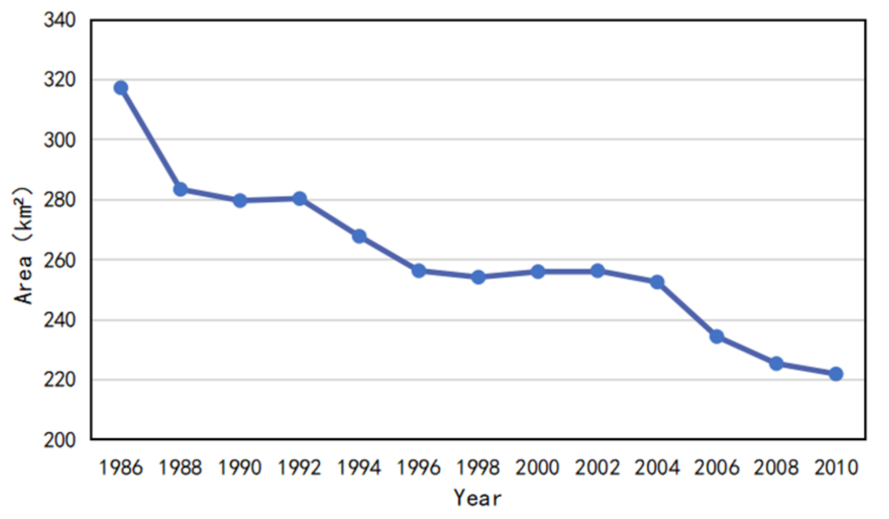
5.1. Interannual Variation of Water Bodies in the Main Urban Area of Hangzhou

To capture the temporal changes of water bodies in the main urban area of Hangzhou, this study quantified the water area by counting the number of water pixels (30 m × 30 m) in the extraction results. The change in water area extracted from 1986 to 2010 is illustrated in Figure 7. The results showed that the total water area in the main urban area of Hangzhou decreased over time. Three obvious periods of change in water body area were observed: (1) 1986–1988: the water body area decreased by 33.85 km²; (2) 1992–1996: the water body area decreased by 12.56 km²; and (3) 2004–2010: the water body area decreased by 30.63 km². It should be noted that the decrease in water area is mainly reflected in the decrease in water bodies in Xixi Wetland and on the eastern side of the Qiantang River. Meanwhile, two plateau periods with unchanged water area can be observed in Figure 7: the water body area stayed at approximately 280 km² from 1988 to 1992 and 255 km² from 1996 to 2004. To more accurately understand the main reasons for the change in water area in the main urban area of Hangzhou, the waters of the Qiantang River and Xixi Wetland were analyzed separately.

5.2. Interannual Variation in Water Bodies in Xixi Wetland

Xixi Wetland is compromised by a rich variety of land use types distributed in the connected waters. This study regards this wetland as a whole as a result of concerns that urbanization mainly intrudes from the border to the internal parts of the wetland and because it is necessary to avoid the impact of extraction error due to very fine-scale water bodies and interruption from various types of land use. A dramatic change in the area of Xixi Wetland occurred from 1990 to 2000 (Figure 8 and Figure 9).

The main and dramatic reduction in water area was observed in the northeastern part of Xixi Wetland, particularly from 1994 to 2000, which corresponds to the city’s westward expansion. The original northeastern area of the wetland had disappeared by 2000. No distinct changes in water area or shape were observed after 2000. The disappearance of water bodies in the northeastern part of Xixi Wetland from 1990 to 2000 accounted for approximately 19% of the total reduction of the water area in the main urban area of Hangzhou at that time.

5.3. Interannual Variation in the Water Body in the Vicinity of the Qiantang River

The water area of the Qiantang River in the main urban area exhibited a significant decreasing trend during the study period, particularly in the eastern part of Qiantang District (Figure 10). Although the changes in the water area of the Qiantang River in the main urban area of Hangzhou may not be as prominent when compared with the entire water area of the Qiantang River, they hold considerable significance in the overall change in the water area of the main urban area of Hangzhou.

Through the interannual analysis of change in water area on the eastern side of the Qiantang River in the main urban area of Hangzhou from 1986 to 2010, it can be found that the water area of the Qiantang River rapidly decreased in the three stages of 1986–1988, 1992–1996, and 2004–2008 (Figure 11), with a total decrease of approximately 78% in the main urban area of Hangzhou.

Specifically, the water area along the bank of the Qiantang River decreased by approximately 36.99 km² from 1986 to 1988, exceeding the reduced area of other water bodies in the main urban areas of Hangzhou during the same period. Between 1992 and 1996, the water body area in this region decreased by 20.69 km², which accounted for approximately 80% of the total decrease in water area in the main urban area of Hangzhou during the same period. Similarly, from 2004 to 2008, the water area here decreased by approximately 13.13 km², representing approximately 50% of the total decrease in water bodies. These findings indicate significant changes in water resource management policy occurred for the Qiantang River beginning in the 1980s.

As a whole, the decrease in water area in the Hangzhou section of the Qiantang River was the main factor causing the change in water area in Hangzhou. During the period 1992–1996, the northeastern part of Xixi Wetland was vanishing under the westward expansion of the city; this decrease in water area cannot be ignored. The total area of water lost on the eastern side of the Qiantang River in Hangzhou contributed to approximately 78% of the total water area reduction from 1986 to 2010 in the main urban area of Hangzhou. The change in the spatial extent of other water bodies accounted for 20% of the total reduction in water area in the main urban areas of Hangzhou.

5.4. Landscape Fragmentation Analysis

In addition to the change in water area, the number of water body patches decreased during urbanization. A landscape fragmentation analysis was performed to assess these changes.

Figure 12 shows that the number of water patches in the main urban area of Hangzhou consistently remained above 1000. From 1986 to 2000, the number of patches exhibited an increasing trend, while from 2000 to 2010, it displayed a decreasing trend. The peak number of patches was recorded in 2000, reaching 1457.

The total patch area, which is synonymous with the total water area, showed a declining pattern between 1986 and 2010. Over the 25-year period, landscape fragmentation exhibited an upward trend, indicating an increase in the number of water patches per square kilometer, or smaller reduction in the number of water patches than in the total water patch area. The intensification of landscape fragmentation and the impairment of water body connectivity were then implied. However, a sudden increase in patches in 1998–2000, followed by a sharp decline starting in 2004, was observed. It is noteworthy that from 20 July to 14 September 2000, at least five typhoons made landfall in Zhejiang Province. The satellite image used for the year 2000 was taken on 17 September, just a few days after the last of these typhoons, Saomai, made landfall. The effects of the typhoons were combined with the astronomical high tide of the Qiantang River, which is world-famous for its very high tide. Therefore, the sudden increase in water patches and areas can be attributed to extreme weather events. In addition, the rapid decline of patch numbers after 2004 is consistent with the rapid disappearance of water areas and the expansion of construction land (Figure 12). The south bank of the Qiantang River should be the main area, with a rapid decline in the number of patches and water area.

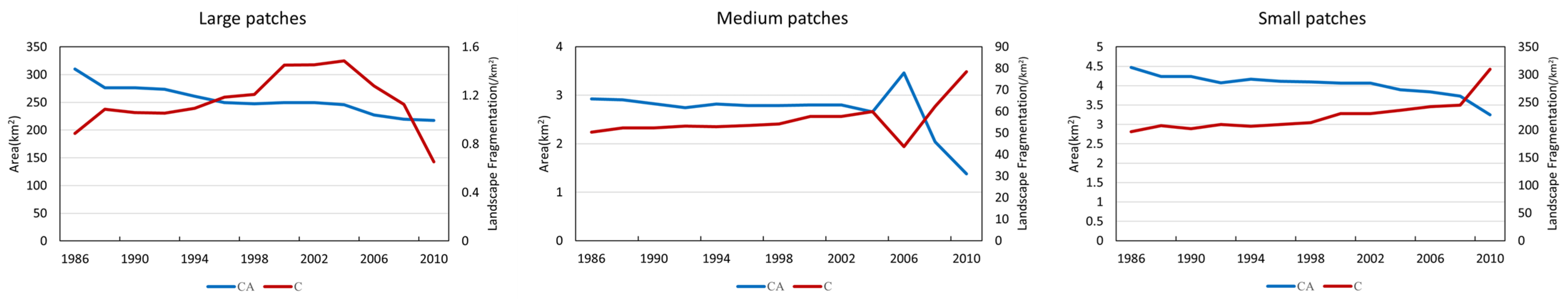
5.4.1. Variation of Landscape Fragmentation with Different Sizes

To observe the impacts on water bodies of different sizes, we classified the bodies into small, medium, and large sizes according to threshold values of 0.005 km², 0.01 km², and 0.01 km². The variation of the water area, patch number, and landscape fragmentation of different sizes were calculated. The results are shown in Figure 13.

It is noted that the change trend of both the water area and patch number is different, corresponding to different sizes of water bodies from 1986 to 2010. The area of large patches continued to decline, but fragmentation increased continuously before 2004 and then began to decline. For patches of medium size, both the area and fragmentation changed slightly, but with a reverse tendency. However, there was a drastic decrease in fragmentation after 2004, followed by a rapid increase after 2006. Whereas the water area showed an inversely drastic change. It is noteworthy that both the area and fragmentation of the small patches basically showed stable and inverse variation; the obvious change was observed in 2008, resulting in an increase in fragmentation degree and a decrease in area.

5.4.2. Variation of Landscape Fragmentation of Water Body in Different Divisions

The landscape fragmentation of water bodies in different divisions of the main urban area of Hangzhou City was calculated and shown in Figure 14.

The landscape fragmentation index in different divisions varied greatly depending on the development degree, respectively. As the traditional center of the main urban area of Hangchou City, Xihu Division, Shangcheng Division, Xiacheng Division, and Gongshu Division changed relatively stable due to the limitations and strict control of development. The fragmentation index of the original Jianggan Division fluctuated greatly, which was closely related to the balance between urbanization and protection of the canal and plain river network during the eastward urbanization of Hangzhou City. In addition, with efficient wetland management and canal dredging and reconstruction, the water area of Gongshu, Shangcheng, and Xiacheng Divisions even increased slightly. It should be noted that the fragmentation index of the Gongshu and Yuhang Divisions was high, but with different causes. The high fragmentation index of Gongshu Division was due to the large number of relatively small water area, whereas the high fragmentation index of Yuhang Division could be attributed to the wide distribution of large ponds or lakes. The patch number was more than 500.

It is noteworthy that the fragmentation index of Yuhang and Xiaoshan Divisions increased, indicating the particularly profound impact of rapid urbanization on the edge of the city. It should be noted that the water area in Xiaoshan Division showed an obvious decline, although it had the largest water area among the eight divisions in Hangzhou. The water area decreased from 198.39 km² in 1986 to 120.10 km² in 2010, while the fragmentation index continuously increased, which indicated the loss of large water bodies during the rapid development. Meanwhile, the water area of Yuhang Division decreased significantly along with its urbanization development, particularly after 2000. The water area decreased by about 45% in 2010 with a distinct increase in fragmentation index.

6. Carbon Footprint Analysis of Water Body Change

6.1. Determination of Carbon Footprint Coefficients

By comprehensively considering the geographical location, climatic zone, and main vegetation types in Hangzhou, the carbon footprint coefficient of each land use type was determined based on previous studies (

Table 5. Carbon footprint coefficients of various land use types.

Land Use Type	Cultivated Land [43]	Woodland [44]	Grassland [44]	Water Area [45]	Unused Land [45]	Construction Land [46]
Carbon footprint coefficient (t·hm−2)	0.497	−0.644	−0.021	−0.218	−0.005	65.300

). Then, based on the calculation of the transformation matrix of land use types, the carbon footprints in the evolution process of water were calculated.

6.2. Land Classification

In this study, the RF classification method was applied to classify the land use types other than water bodies. It is worth noting that water body extraction for Landsat data was performed every year from 1985 to 2010 in this study; both land type classification of all types analyzed here and water body extraction were performed in the same year. To highlight the changes in land use over time, Landsat 5/TM images were selected every 5 years from 1985 to 2010 for the classification; the results are shown in Figure 15.

A Kappa coefficient was used to verify the classification results, and its calculation formula is as follows:

$$\mathrm{Kappa}=\frac{P_0-P_e}{1-P_e}$$

(13)

In the above formula,

$${\mathrm{P}}_0=\frac{\mathrm{TP}+\mathrm{TN}}{{\mathrm{N}}^2}$$

(14)

$${\mathrm{P}}_{\mathrm{e}}=\frac{\left(\mathrm{TP}+\mathrm{FP}\right)\times \left(\mathrm{TP}+\mathrm{FN}\right)+\left(\mathrm{TN}+\mathrm{FN}\right)\times \left(\mathrm{TN}+\mathrm{FP}\right)}{{\mathrm{N}}^2}$$

(15)

where N is the total number of pixels. The accuracy of the Kappa coefficient was 88%, indicating reliable classification. As shown in Figure 13, cultivated land covers the largest part of the main urban area of Hangzhou, while woodland is predominantly located in the peripheral areas. Grassland and unused land occupy a relatively small area, while the construction land is primarily concentrated along both sides of the Qiantang River, and its area has been expanding over time.

6.3. Transformation of Water Bodies into Other Types of Land and Related Calculations

The transformation of water areas can be classified into two cases: (1) the transformation of water areas into other land use types; and (2) the transformation of other land use types into water areas. By aggregating the conversion areas in both directions, the net conversion areas for each land use type and water area can be obtained, as presented in

Table 6. Net conversion areas (km²) of water bodies to five land use types.

Year	Land Use Types
	Cultivated Land	Woodland	Grassland	Construction Land	Unused Land
1985–1990	3756	−12	−1	18	0.00
1990–1995	1134	−15	0.00	134	0.00
1995–2000	971	−24	5	203	0.00
2000–2005	1768	56	11	334	0.18
2005–2010	1160	2	1	39	−2

.

As shown in Table 6, the conversion area between water bodies and cultivated land was the largest, exceeding 90% during the periods 1985–1990 and 2005–2010. This conversion mainly occurred on the eastern side of the Qiantang River, where most water bodies were transformed into cultivated land. This situation is quite similar to that on the southern bank of Hangzhou Bay [47]. Additionally, the water area in the eastern Xixi Wetland was primarily converted into construction land. The decrease in water bodies in these two regions significantly contributed to the changes in land use.

6.4. Analysis of Carbon Footprint Change in Water Body Transformation

According to the carbon footprint coefficients for different types of land use and the conversion area between water area and other land use types in Section 5.1, the carbon footprint of land use in each period was estimated. The estimation formula is as follows:

$${\mathrm{C}}_e={\displaystyle \sum }{A}_i\times \left(a_i-a_w\right)$$

(16)

where C_e is the carbon footprint of land use type i; A_i is the area of land use type i (cultivated land, woodland, grassland, unused land, and construction land); a_i is the carbon footprint coefficient of land use type i; and a_w is the carbon footprint coefficient of water bodies.

According to Equation (16), the carbon footprint change caused by land use type transformation every 5 years from 1985 to 2010 was calculated, and the results are shown in

Table 7. Changes in carbon footprint from water bodies compared to other land use types.

Year	1985–1990	1990–1995	1995–2000	2000−2005	2005−2010
Carbon footprint/t	3068	9324	13,762	23,521	3096

.

The carbon footprints resulting from the transformation of water areas increased during each 5-year period from 1985 to 2005 (Table 7), which is consistent with the water areas converted into urbanized areas, which also increased during this period (Table 6). These findings indicate that the transformation of water bodies into urbanized areas contributed the most to the carbon footprint among all land use type changes. It is noteworthy that the change in carbon footprint from 2005 to 2010 exhibited a moderating trend. Correspondingly, the transformation of water bodies into construction land was minimal during this period (Table 6).

In summary, the transformation of the water area into construction land contributed significantly to the increase of the carbon footprint of Hangzhou. From 1985 to 2005, due to the process of urbanization, the water area converted into construction land increased in Hangzhou, which led to a continuous increase in the carbon footprint, an increase that peaked from 2000 to 2005. From 2005 to 2010, the area of water converted to construction land decreased, resulting in a reduced carbon footprint.

6.5. Correlation Analysis of Landscape Fragmentation and Carbon Footprint

Distinctly different change patterns between landscape fragmentation and carbon emissions were observed in the main urban area of Hangzhou (Figure 16). Landscape fragmentation continued to increase during the period 1988–2000, followed by a sudden increase during the period 1998–2000, which meant landscape fragmentation peaked at a high level during the period 2000–2010. The change in landscape fragmentation showed little fluctuation between 5.66 and 5.84 after 2010. In comparison, the change in carbon footprint continued to increase during the period 1985–2005 and reached a maximum during the period 2000–2005. Through comparison, it was found that the change in landscape fragmentation in the main urban area of Hangzhou suddenly intensified during the period 1998–2000, and the connectivity of water bodies in the urban area decreased, which led to a deterioration in water quality. Eutrophication and poor water quality easily lead to anaerobic conditions in water bodies and increase their carbon footprint, which may also be one of the reasons for the increase in the carbon footprint from 2000 to 2005.

7. Conclusions

This study used Landsat 5/TM imagery to extract water bodies in the main urban area of Hangzhou from 1986 to 2010. The changes in the area, number of patches, and landscape fragmentation of water bodies were analyzed to reveal the impact of recent rapid urbanization. Carbon footprint changes associated with the transformation between water and other land uses were also calculated. The study reached the following conclusions:

Based on the U-Net deep learning algorithm, a combined loss function incorporating both Focal and Dice Losses was employed to improve the accuracy of small water body extraction from Landsat 5/TM images with 30 m spatial resolution. The classification accuracy achieved by the U-Net model reached 94.3%. In addition, the RF classification method combined with a U-Net water body extraction model was used to classify the land use of the main urban area of Hangzhou. The RF classification accuracy can reach 88%, apart from the classification of water bodies.

The reduction of water area in the main urban area of Hangzhou primarily occurred between 1986 and 2010. The main factors contributing to this reduction were the Qiantang River reclamation and encroachment on the Xixi Wetland during urban expansion. Qiantang River reclamation was most prominent from 1986 to 1988, accounting for most of the reduction in urban water areas in Hangzhou. The decline in the spatial extent of Xixi Wetland was significant from 1990 to 2000 and was mainly concentrated in the northeast region. The decrease in the spatial extent of Xixi Wetland accounted for 19% of the total water body reduction in Hangzhou. Large patches of water bodies, such as natural lakes and big rivers, located at the edge of the city are susceptible to disappearing during the rapid outward expansion. However, due to the limitations and strict control of development, water bodies, referred to as wetland, slender canals, and plain river networks, in the traditional center division of the city, are preserved well.

The conversion between water bodies and cultivated land was most significant, followed by the conversion between water bodies and construction land. Notably, the conversion of water areas to particularly construction land resulted in an increasing carbon footprint, which accounted for over 90% of the total carbon footprint increase caused by land use change. In particular, the transformation of water bodies into construction land, especially in the context of Xixi Wetland, accounted for one of the critical factors inducing the change in carbon footprint during the urbanization period.

The findings of this research have important implications for the effective management of urban water resources, the protection of urban aquatic ecosystems, and accurately estimating regional dual-carbon targets.

References

1. Yang, X.; Qin, Q.; Grussenmeyer, P.; Koehl, M. Urban surface water body detection with suppressed built-up noise based on water indices from Sentinel-2 MSI imagery. Remote Sens. Environ. 2018, 219, 259–270. [Google Scholar] [CrossRef]
2. Wang, H.; Li, C. Analysis of scale effect and change characteristics of ecological landscape pattern in urban waters. Arab. J. Geosci. 2021, 14, 569. [Google Scholar] [CrossRef]
3. Steele, M.K.; Heffernan, J.B. Morphological characteristics of urban water bodies: Mechanisms of change and implications for ecosystem function. Ecol. Appl. 2014, 24, 1070–1084. [Google Scholar] [CrossRef]
4. Chen, L.; Zhou, B.; Man, W.; Liu, M. Landsat-Based Monitoring of the Heat Effects of Urbanization Directions and Types in Hangzhou City from 2000 to 2020. Remote Sens. 2021, 13, 4268. [Google Scholar] [CrossRef]
5. Bartolucci, L.A.; Robinson, B.F.; Silva, L.F. Field measurements of the spectral response of natural waters. Photogramm. Eng. Remote Sens. 1977, 43, 595–598. [Google Scholar]
6. Shamsuzzoha, M.; Ahamed, T. Shoreline Change Assessment in the Coastal Region of Bangladesh Delta Using Tasseled Cap Transformation from Satellite Remote Sensing Dataset. Remote Sens. 2023, 15, 295. [Google Scholar] [CrossRef]
7. Yao, J.; Sun, S.; Zhai, H.; Feger, K.-H.; Zhang, L.; Tang, X.; Li, G.; Wang, Q. Dynamic monitoring of the largest reservoir in North China based on multi-source satellite remote sensing from 2013 to 2022: Water area, water level, water storage and water quality. Ecol. Indic. 2022, 144, 109470. [Google Scholar] [CrossRef]
8. Yang, L.; Tian, S.; Yu, L.; Ye, F.; Qian, J.; Qian, Y. Deep learning for extracting water body from Landsat imagery. Int. J. Innov. Comput. Inf. Control 2015, 11, 1913–1929. [Google Scholar]
9. Chen, J.; Zhu, W.; Tian, Y.Q.; Yu, Q. Monitoring dissolved organic carbon by combining Landsat-8 and Sentinel-2 satellites: Case study in Saginaw River estuary, Lake Huron. Sci. Total Environ. 2020, 718, 137374. [Google Scholar] [CrossRef]
10. Xia, H.; Zhao, J.; Qin, Y.; Yang, J.; Cui, Y.; Song, H.; Ma, L.; Jin, N.; Meng, Q. Changes in water surface area during 1989–2017 in the Huai River Basin using Landsat data and Google earth engine. Remote Sens. 2019, 11, 1824. [Google Scholar] [CrossRef]
11. Du, J.; Kimball, J.S.; Galantowicz, J.; Kim, S.B.; Chan, S.K.; Reichle, R.; Jones, L.A.; Watts, J.D. Assessing global surface water inundation dynamics using combined satellite information from SMAP, AMSR2 and Landsat. Remote Sens. Environ. 2018, 213, 1–17. [Google Scholar] [CrossRef] [PubMed]
12. Deng, Y.; Jiang, W.; Tang, Z.; Li, J.; Lv, J.; Chen, Z.; Jia, K. Spatio-temporal change of lake water extent in Wuhan urban agglomeration based on Landsat images from 1987 to 2015. Remote Sens. 2017, 9, 270. [Google Scholar] [CrossRef]
13. Fisher, A.; Flood, N.; Danaher, T. Comparing Landsat water index methods for automated water classification in eastern Australia. Remote Sens. Environ. 2016, 175, 167–182. [Google Scholar] [CrossRef]
14. Li, Y.; Gong, X.; Guo, Z.; Xu, K.; Hu, D.; Zhou, H. An index and approach for water extraction using Landsat–OLI data. Int. J. Remote Sens. 2016, 37, 3611–3635. [Google Scholar] [CrossRef]
15. Feng, S.; Fan, F. Impervious surface extraction based on different methods from multiple spatial resolution images: A comprehensive comparison. Int. J. Digit. Earth 2021, 14, 1148–1174. [Google Scholar] [CrossRef]
16. Li, L.; Su, H.; Du, Q.; Wu, T. A novel surface water index using local background information for long term and large-scale Landsat images. ISPRS J. Photogramm. Remote Sens. 2021, 172, 59–78. [Google Scholar] [CrossRef]
17. Peng, J.; Li, L.; Tang, Y.Y. Maximum Likelihood Estimation-Based Joint Sparse Representation for the Classification of Hyperspectral Remote Sensing Images. IEEE Trans. Neural Netw. Learn. Syst. 2019, 30, 1790–1802. [Google Scholar] [CrossRef] [PubMed]
18. Gandhimathi Alias Usha, S.; Vasuki, S. Improved segmentation and change detection of multi-spectral satellite imagery using graph cut based clustering and multiclass SVM. Multimed. Tools Appl. 2017, 77, 15353–15383. [Google Scholar] [CrossRef]
19. Wang, Y.; Li, Z.; Zeng, C.; Xia, G.-S.; Shen, H. An urban water extraction method combining deep learning and Google Earth engine. IEEE J. Sel. Top. Appl. Earth Obs. Remote Sens. 2020, 13, 769–782. [Google Scholar] [CrossRef]
20. Zhang, Y.; Gao, J.; Wang, J. Detailed mapping of a salt farm from Landsat TM imagery using neural network and maximum likelihood classifiers: A comparison. Int. J. Remote Sens. 2007, 28, 2077–2089. [Google Scholar] [CrossRef]
21. Ko, B.C.; Kim, H.H.; Nam, J.Y. Classification of Potential Water Bodies Using Landsat 8 OLI and a Combination of Two Boosted Random Forest Classifiers. Sensors 2015, 15, 13763–13777. [Google Scholar] [CrossRef] [PubMed]
22. Shi, Y.; Qi, Z.; Liu, X.; Niu, N.; Zhang, H. Urban land use and land cover classification using multisource remote sensing images and social media data. Remote Sens. 2019, 11, 2719. [Google Scholar] [CrossRef]
23. Konapala, G.; Kumar, S.V.; Ahmad, S.K. Exploring Sentinel-1 and Sentinel-2 diversity for flood inundation mapping using deep learning. ISPRS J. Photogramm. Remote Sens. 2021, 180, 163–173. [Google Scholar] [CrossRef]
24. Rezaee, M.; Mahdianpari, M.; Zhang, Y.; Salehi, B. Deep convolutional neural network for complex wetland classification using optical remote sensing imagery. IEEE J. Sel. Top. Appl. Earth Obs. Remote Sens. 2018, 11, 3030–3039. [Google Scholar] [CrossRef]
25. Xia, M.; Qian, J.; Zhang, X.; Liu, J.; Xu, Y. River segmentation based on separable attention residual network. J. Appl. Remote Sens. 2020, 14, 032602. [Google Scholar] [CrossRef]
26. Wu, F.; Wang, C.; Zhang, H.; Li, J.; Li, L.; Chen, W.; Zhang, B. Built-up area mapping in China from GF-3 SAR imagery based on the framework of deep learning. Remote Sens. Environ. 2021, 262, 112515. [Google Scholar] [CrossRef]
27. Siddique, N.; Paheding, S.; Elkin, C.P.; Devabhaktuni, V. U-net and its variants for medical image segmentation: A review of theory and applications. IEEE Access 2021, 9, 82031–82057. [Google Scholar] [CrossRef]
28. Li, F.; Sun, W.; Yang, G.; Weng, Q. Investigating spatiotemporal patterns of surface urban heat islands in the Hangzhou Metropolitan Area, China, 2000–2015. Remote Sens. 2019, 11, 1553. [Google Scholar] [CrossRef]
29. Lin, Y.; Jim, C.Y.; Deng, J.; Wang, Z. Urbanization effect on spatiotemporal thermal patterns and changes in Hangzhou (China). Build. Environ. 2018, 145, 166–176. [Google Scholar] [CrossRef]
30. Du, N.; Ottens, H.; Sliuzas, R. Spatial impact of urban expansion on surface water bodies—A case study of Wuhan, China. Landsc. Urban Plan. 2010, 94, 175–185. [Google Scholar] [CrossRef]
31. Cobbinah, P.B.; Korah, P.I.; Bardoe, J.B.; Darkwah, R.M.; Nunbogu, A.M. Contested urban spaces in unplanned urbanization: Wetlands under siege. Cities 2022, 121, 103489. [Google Scholar] [CrossRef]
32. Kuang, W.; Liu, J.; Dong, J.; Chi, W.; Zhang, C. The rapid and massive urban and industrial land expansions in China between 1990 and 2010: A CLUD-based analysis of their trajectories, patterns, and drivers. Landsc. Urban Plan. 2016, 145, 21–33. [Google Scholar] [CrossRef]
33. Goodchild, M.F. Citizens as sensors: The world of volunteered geography. GeoJournal 2007, 69, 211–221. [Google Scholar] [CrossRef]
34. Neis, P.; Zipf, A. Analyzing the contributor activity of a volunteered geographic information project—The case of OpenStreetMap. ISPRS Int. J. Geo-Inf. 2012, 1, 146–165. [Google Scholar] [CrossRef]
35. Haklay, M. How good is volunteered geographical information? A comparative study of OpenStreetMap and Ordnance Survey datasets. Environ. Plan. B Plan. Des. 2010, 37, 682–703. [Google Scholar] [CrossRef]
36. Goodfellow, I.J.; Shlens, J.; Szegedy, C. Explaining and harnessing adversarial examples. arXiv 2014, arXiv:1412.6572. [Google Scholar]
37. Lin, T.-Y.; Goyal, P.; Girshick, R.; He, K.; Dollár, P. Focal loss for dense object detection. In Proceedings of the IEEE International Conference on Computer Vision, Venice, Italy, 22–29 October 2017; pp. 2980–2988. [Google Scholar]
38. Zhu, Z.; Liu, C.; Yang, D.; Yuille, A.; Xu, D. V-NAS: Neural architecture search for volumetric medical image segmentation. In Proceedings of the 2019 International Conference on 3D Vision (3DV), Québec, QC, Canada, 16–19 September 2019; pp. 240–248. [Google Scholar]
39. Barton, I.J.; Bathols, J.M. Monitoring floods with AVHRR. Remote Sens. Environ. 1989, 30, 89–94. [Google Scholar] [CrossRef]
40. Xu, H. Modification of normalised difference water index (NDWI) to enhance open water features in remotely sensed imagery. Int. J. Remote Sens. 2006, 27, 3025–3033. [Google Scholar] [CrossRef]
41. Maulik, U.; Chakraborty, D. Learning with transductive SVM for semisupervised pixel classification of remote sensing imagery. ISPRS J. Photogramm. Remote Sens. 2013, 77, 66–78. [Google Scholar] [CrossRef]
42. GB/T 21010-2007; Current Land Use Classification. General Administration of Quality Supervision, Inspection and Quarantine of the PRC, and Standardization Administration of the PRC: Beijing, China, 2007.
43. Cai, Z.; Kang, G.; Tsuruta, H.; Mosier, A. Estimate of CH4 Emissions from Year-Round Flooded Rice Fields During Rice Growing Season in China. Pedosphere 2005, 15, 66–71. [Google Scholar]
44. Fang, J.; Piao, S.; Field, C.B.; Pan, Y.; Guo, Q.; Zhou, L.; Peng, C.; Tao, S. Increasing net primary production in China from 1982 to 1999. Front. Ecol. Environ. 2003, 1, 293–297. [Google Scholar] [CrossRef]
45. Lai, L.; Huang, X.J. Environmental cost accounting of chemical fertilizer utilization in China. In Proceedings of the 2008 2nd International Conference on Bioinformatics and Biomedical Engineering, Shanghai, China, 16–18 May 2008; pp. 4229–4232. [Google Scholar]
46. Luijten, J. A systematic method for generating land use patterns using stochastic rules and basic landscape characteristics: Results for a Colombian hillside watershed. Agric. Ecosyst. Environ. 2003, 95, 427–441. [Google Scholar] [CrossRef]
47. Liang, J.; Chen, C.; Song, Y.; Sun, W.; Gang Yang, G. Long-term mapping of land use and cover changes using Landsat images on the Google Earth Engine Cloud Platform in bay area—A case study of Hangzhou Bay, China. Sustain. Horiz. 2023, 7, 100061–100081. [Google Scholar] [CrossRef]
Figure 1. (a) Location of Hangzhou City (indicated by a red dot ●) on a digital elevation map including Anhui, Jiangsu, and Zhejiang Provinces and Shanghai City within the Yangtze River Delta; the map comes from the US National Aeronautics and Space Administration’s Shuttle Radar Topography Mission and has a 90 m resolution. (b) For administrative divisions of Hangzhou in 2021, data is sourced from the National Geographic Information Resources Directory Service.
Remotesensing 16 02579 g001
Figure 2. The technical roadmap of this study. Note: MNDWI, modified normalized difference water index; AWEI, automated water body extraction index (AWEI); SVM, support vector machine; and OSM, OpenStreetMap software.
Remotesensing 16 02579 g002
Figure 3. Labelling data of the water body for Hangzhou City that aligns with the satellite images: (a) original Landsat 5/Thematic Mapper image of Hangzhou City in 2010; (b) labeling data of the water body processed by ArcGIS.
Remotesensing 16 02579 g003
Figure 4. Training process of water body extraction algorithm based on the U-Net model. Note: OSM, OpenStreetMap platform.
Remotesensing 16 02579 g004
Figure 5. Comparison of water body extraction results by different methods: (a) the original Land-sat5/Thematic Mapper image acquired in 2010; (b) modified normalized difference water index; (c) automated water body extraction index; (d) SVM; and (e) U-Net.
Remotesensing 16 02579 g005
Figure 6. Water body extraction results of the U-Net model every 2 years from 1986 to 2010 are shown in (am), respectively.
Remotesensing 16 02579 g006
Figure 7. Biennial changes of water area from 1986 to 2010 in the main urban area of Hangzhou, Zhejiang, China.
Remotesensing 16 02579 g007
Figure 8. Water body extraction from Xixi Wetland every 2 years from 1990 to 2000 is shown in (af), respectively.
Remotesensing 16 02579 g008
Figure 9. Reduction of water area of Xixi Wetland every 2 years from 1990 to 2000.
Remotesensing 16 02579 g009
Figure 10. Tailored Landsat5/Thematic Mapper image where the Qiantang River meanders through Zhejiang Province. The red square represents part of the main urban area of Hangzhou, where the Qiantang River flows. The blue shading represents the section of the Qiantang River with dramatic change.
Remotesensing 16 02579 g010
Figure 11. Significant variation in the water area in the eastern side of the Qiantang River in the main urban area of Hangzhou in (a) 1986–1988, (b) 1992–1996, (c) 2004–2008, and (d) Graph of the biennial changes in the water area of the Qiantang River in the main urban area of Hangzhou City from 1986 to 2010.
Remotesensing 16 02579 g011
Figure 12. Graph of the biennial changes in the number of water body patches and landscape fragmentation from 1986 to 2010.
Remotesensing 16 02579 g012
Figure 13. The variation of both the water area and fragmentation with different sizes.
Remotesensing 16 02579 g013
Figure 14. The variation of both the water area and fragmentation in different divisions.
Remotesensing 16 02579 g014
Figure 15. Land use classification results every 5 years from 1985 to 2020 are shown in (af), respectively.
Remotesensing 16 02579 g015
Figure 16. Biennial changes in (a) landscape fragmentation and (b) carbon footprint from 1985 to 2010.
Remotesensing 16 02579 g016