Imaging Seafloor Features Using Multipath Arrival Structures

Abstract

In this paper, we propose an imaging method for seafloor features based on multipath arrival structures. The bistatic sonar system employed consists of a vertical transmitting array and a horizontal towed array. The conventional back projection (BP) method, which considers the direct path from the source to the seafloor scatterer and then to the receiver, is used in this system. However, discrepancies between the calculated delay values and the actual propagation delay result in projection deviations and offsets in the seafloor features within sound intensity images. To address this issue, we analyze the multipath structures from the source to the scatterer and then to the receiver based on ray theory. The delay at each grid is calculated using different multipaths, considering the distances from the seafloor grids to the source and the receiver. In the direct zone, the delay is determined using the direct ray and the surface reflection ray, while in the bottom bounce area, the delay is calculated using the bottom–surface reflection ray and the surface–bottom–surface reflection ray. Numerical simulations and experimental results demonstrate that the proposed method rectifies the delay calculation issues inherent in the conventional method. This adjustment enhances the accuracy of the projection, thereby improving the imaging quality of seafloor features.

1. Introduction

Underwater acoustic imaging is crucial for obtaining ocean environment information, which provides guidance for underwater navigation and resource exploration through the visualization of seabed characteristics. Traditional equipment, such as side-scan sonar and multi-beam bathymetric sonar, usually generate striped seafloor images. In contrast, the ocean acoustic waveguide remote sensing (OAWRS) system [1,2], consisting of a vertical transmitting array and a horizontal towed array, collects a wide range of oceanographic information on a large spatial scale. This system utilizes the characteristics of acoustic propagation in the marine environment, including the existence of acoustic channels and waveguide modes. Specifically, the OAWRS system can perform wide-area imaging in the range of tens of kilometers, providing visualizations of islands [3,4,5], volcanoes, and fish shoals [6,7,8,9,10,11,12], as well as marine mammals [13,14], which is attracting increasing attention.

Previous studies have shown a relationship between seafloor topography and the intensity of scattered signals [15,16,17,18,19]. Following the beamforming of received data from the horizontal array, coordinate transformation was performed to determine the origin of scattered echoes by comparing it with the bathymetry. Data obtained during experiments at the Mid-Atlantic Ridge (MAR) indicated that prominent echoes emanate from steep slopes, and that the left–right ambiguity of the horizontal array is distinguished by considering propagation losses [16,17]. Furthermore, researchers employed a long-range bistatic sonar system to conduct single and bistatic imaging experiments in the continental shelf region [20,21,22]. By multiplying the beam output data by half of the measured sound speed, they were converted into beam range data. Afterwards, the beam range data were projected to a Cartesian coordinate grid to image the features of a preset inflatable tubular target and subsurface river channel. Additionally, Preston and Ellis [23,24,25] processed towed array data into beam data, and overlaid polar scattering plots of the beam outputs on the bathymetry to distinguish unknown seafloor features by comparing the model and data results. Considering the impact of propagation loss, the minimum echo intensity at each moment was regarded as background and then subtracted from the original image [26,27,28]. The imaging results corresponded to rocks, shipwrecks, and ridges.

However, in the aforementioned studies, several problems exist in the conventional back projection (BP) method [29] used to project the beam outputs to the seafloor grid. Firstly, to simplify calculations in shallow water, the horizontal distance is employed instead of the true acoustic path. Secondly, with this approach, the effects of multipath propagation are often disregarded in deep-water environments, with only the direct path from the source to the seafloor and then to the receiver being considered. These simplifications result in inaccurate acoustic distance estimations, thus leading to discrepancies between the calculated delay and the true propagation time of the signal. Consequently, this lack of precision can cause misalignment in the projection process, thereby impacting the accuracy of seafloor feature detection and recognition.

In this paper, a back projection imaging method based on multipath arrival structures (MAS-BP) is proposed. According to the range between the seafloor grid and the source, as well as the receiver, we employ various eigenrays for delay calculation to enhance the accuracy of projection processing. The effectiveness of this approach is confirmed by theoretical derivation and numerical simulations. Additionally, the proposed method is applied to process the experimental data. By comparing the bathymetry with the generated sound intensity image, the efficacy of the proposed method in reducing position deviation is confirmed.

This paper is organized as follows: Section 2 introduces the receiving signal model and its simplification. Section 3 presents the imaging method based on multipath structures and a comparison with the conventional method. Section 4 shows the numerical simulations and Section 5 presents the experimental results. Finally, Section 6 summarizes the conclusions.

2. Receiving Signal Model

2.1. General Form of Receiving Signal Model

A bistatic sonar system for imaging seafloor features composed of a vertical transmitting array and a horizontal receiving array is considered, and an acoustic imaging scene is shown in Figure 1. The signal from the vertical transmitting array is scattered across the seafloor and received by the towed array during each transmission, and then a seafloor image of the received sound pressure level is generated for every transmission.

It is assumed that the depth of the water is denoted as H and that the sound speed is c. The center coordinate of the $L_S$-element vertical transmitting array is $\left(x_{\mathrm{S}},y_{\mathrm{S}},z_{\mathrm{S}}\right)$, with an element spacing of $d_{\mathrm{S}}$. The first element of the $L_{\mathrm{R}}$-element horizontal receiving array with an element spacing of $d_{\mathrm{R}}$ is set as the reference, and its coordinate is $\left(x_{\mathrm{R}},y_{\mathrm{R}},z_{\mathrm{R}}\right)$. The normal direction of the vertical array and that of the horizontal array are denoted as 0°, and the clockwise direction corresponds to the positive angle of the transmitting beam. The receiving beam angle is denoted as −90° when pointing to the No. 1 element, and it is denoted as 90° when pointing to the last array element. The heading angle of the receiving array is $\gamma$. The heading angle mentioned in this paper is defined as 0° in the positive direction of the x-axis, and the positive angle is in the counterclockwise direction.

For a bistatic sonar, the incident plane and the scattering plane are typically not in the same plane. Consequently, a three-dimensional scattering function $g\left({\alpha }_{\mathrm{inc}},{\alpha }_{\mathrm{scatt}},\phi \right)$ is employed to describe the seabed scattering. Assume that the coordinate of the scatterer on the unit area of the seafloor is $\left(x_i,y_i,z_i\right),i=1,2,\dots ,K.$ Moreover, its horizontal distance to the center of the transmitting array and the reference element of the receiving array are $r_{\mathrm{S}i}$ and $r_{\mathrm{R}i}$, respectively. The grazing angle of the eigenray at the source and that at the receiver are denoted as ${\beta }_{\mathrm{S}}$ and ${\beta }_{\mathrm{R}}$. ${\alpha }_{\mathrm{inc}}$, ${\alpha }_{\mathrm{scatt}}$, and ${\phi }_i$ represent the incident grazing angle, the scattered grazing angle, and the scattered azimuth angle, respectively. Meanwhile, ${\theta }_i$ represents the angle between the scattering plane and the normal direction of the receiving array.

According to ray theory, the received signal of the lth element of the receiving array can be expressed as:

$$p_l\left(t\right)={\displaystyle \sum _{m=1}^M{\displaystyle \sum _{n=1}^N{A}_{\mathrm{inc},m}{A}_{\mathrm{scatt},n}{B}_{\mathrm{S}}\left({\beta }_{\mathrm{S}m};{\theta }_{\mathrm{S}}\right)}}s\left(t-{\tau }_{\mathrm{inc},m}-{\tau }_{\mathrm{scatt},n}\right)e^{-j\omega \left(l-1\right)d_{\mathrm{R}}\sin {{\theta }^{\prime }}_{i,n}/c}$$

(1)

where $s\left(t\right)$ represents the transmitting signal, $\omega =2\pi f$ is the angular frequency, and f is the frequency of the source. $B_{\mathrm{S}}\left({\beta }_{Sm};{\theta }_{\mathrm{S}}\right)$ is the beam pattern function of the transmitting array, where ${\theta }_{\mathrm{S}}$ denotes the angle of the transmitting beam. The meanings of the other parameters in Equation (1) are as follows:

• M and N: the number of incident eigenrays and the number of scattered eigenrays.
• $A_{\mathrm{inc},m}$ and ${\tau }_{\mathrm{inc},m}$: the amplitude and propagation delay of the mth incident eigenray.
• $A_{\mathrm{scatt},n}$ and ${\tau }_{\mathrm{scatt},n}$: the amplitude and propagation delay of the nth scattered eigenray.
• ${\alpha }_{\mathrm{inc},m}$ and ${\alpha }_{\mathrm{scatt},n}$: the incident grazing angle of the mth incident eigenray and the scattered grazing angle of the nth scattered eigenray.
• ${{\theta }^{\prime }}_{i,n}$: the direction of the arrival angle of the nth scattered eigenray, where $\sin {{\theta }^{\prime }}_{i,n}=\sin {\theta }_i\cos {\beta }_{\mathrm{R}n}$.

The equations for the amplitude and the propagation delay are as follows:

$$\left\{\begin{array}{l}{A}_{\mathrm{inc},m}=\sqrt{\frac{W\cos {\beta }_{\mathrm{S}m}}{r_{\mathrm{S}i}{\left|\partial r_{\mathrm{S}i}/\partial {\beta }_{\mathrm{S}m}\right|}_{{\beta }_{\mathrm{S}m}}\sin {\alpha }_{\mathrm{inc},m}}}\\ {\tau }_{\mathrm{inc},m}=\left(r_{\mathrm{S}i}\cos {\beta }_{\mathrm{S}m}+{\displaystyle {\int }_{z_{\mathrm{S}}}^H\sqrt{{\eta }^2\left(z\right)-{\cos }^2{\beta }_{\mathrm{S}m}}dz}\right)/c\end{array}\right.$$

(2)

$$\left\{\begin{array}{l}{A}_{\mathrm{scatt},n}=\sqrt{\frac{W\cos {\beta }_{\mathrm{R}n}}{r_{\mathrm{R}i}{\left|\partial r_{\mathrm{R}i}/\partial {\beta }_{\mathrm{R}n}\right|}_{{\beta }_{\mathrm{R}n}}\sin {\alpha }_{\mathrm{scatt},n}}}\\ {\tau }_{\mathrm{scatt},n}=\left(r_{\mathrm{R}i}\cos {\beta }_{\mathrm{R}n}+{\displaystyle {\int }_{z_{\mathrm{R}}}^H\sqrt{{\eta }^2\left(z\right)-{\cos }^2{\beta }_{\mathrm{R}n}}dz}\right)/c\end{array}\right.$$

(3)

where W represents the radiated power per unit solid angle and $\eta \left(z\right)=c\left(z\right)/c\left(z_{\mathrm{S}}\right)$ is the refractive rate. In this research, we employ the Bellhop ray model to compute the amplitude and propagation delay of the eigenrays.

Using the conventional scattering model in references [30,31], the three-dimensional scattering function $g\left({\alpha }_{\mathrm{inc}},{\alpha }_{\mathrm{scatt}},\phi \right)$ is expressed as:

$$G\left({\alpha }_{\mathrm{inc},m},{\alpha }_{\mathrm{scatt},n},{\phi }_i\right)={\left|g\left({\alpha }_{\mathrm{inc},m},{\alpha }_{\mathrm{scatt},n},{\phi }_i\right)\right|}^2=\mu {\alpha }_{\mathrm{inc},m}{\alpha }_{\mathrm{scatt},n}+\nu {\left(1+\Delta \Omega \right)}^2{e}^{\frac{-\Delta \Omega }{2{\sigma }^2}}$$

(4)

$$\Delta \Omega =\frac{{\cos }^2{\alpha }_{\mathrm{inc},m}+{\cos }^2{\alpha }_{\mathrm{scatt},n}-2\cos {\alpha }_{\mathrm{inc},m}\cos {\alpha }_{\mathrm{scatt},n}\cos {\phi }_i}{{\left(\sin {\alpha }_{\mathrm{inc},m}+\sin {\alpha }_{\mathrm{scatt},n}\right)}^2}$$

(5)

where $\mu$ represents the backscattering intensity, $\nu$ is the lateral scattering intensity, $\sigma$ is the lateral scattering deviation, and $\Delta \Omega$ denotes the deviation between the scattered eigenray and the mirror reflection direction (${\phi }_i=0^{\circ }$).

2.2. Simplification of the Receiving Signal Model

Since the energy of the secondary and multiple reflected rays is weak, the received signal model is simplified by analyzing the multipath structure in this section. Ignoring the secondary reflected rays, only four types of rays between the sound source or receiver and the scatterer are considered, which are the direct ray (DR), surface reflection ray (SR), bottom–surface reflection ray (BSR), and surface–bottom–surface reflection ray (SBSR).

The Bellhop ray model can be utilized to compute the eigenray path in the seafloor grid. Based on the horizontal distance from the source or receiver to the seafloor grid, we can calculate the presence of the DR or SR. This outcome is employed to distinguish between the seafloor grid located within the direct zone or the bottom bounce zone. In scenarios where the distance between the seafloor scatterer and the source or the receiver is relatively short, the SR and DR are the primary rays. When the scatterer is situated in the bottom bounce zone, the BSR and SBSR become the predominant rays.

The multipath structures from the source to the seafloor scatterer and then to the receiver are shown in Figure 2. Depending on the distance from the scatterer to the sound source and receiver, there are four types of multipath structures: (a) SR/DR-SR/DR; (b) SR/DR-BSR/SBSR; (c) BSR/SBSR-SR/DR; and (d) BSR/SBSR-BSR/SBSR. Consequently, the incident rays and scattered rays in Equation (1) are simplified into two rays.

Figure 3 shows the eigenray path between the source and the scatterer, as well as the changes in exit angle at the source with the distance and those in the incident grazing angle at the scatterer, when the scatterer is in different locations. As illustrated in Figure 3, exit angles ${\beta }_{\mathrm{S}1}$ and ${\beta }_{\mathrm{S}2}$ are approximately equal, indicating that ${\beta }_{\mathrm{S}1}\approx \left|{\beta }_{\mathrm{S}2}\right|\approx {\overline{\beta }}_{\mathrm{S}}$. Similarly, the incident grazing angles, named ${\alpha }_{\mathrm{inc},1}$ and ${\alpha }_{\mathrm{inc},2}$, of the two rays are also approximately equal, demonstrating that ${\alpha }_{\mathrm{inc},1}\approx {\alpha }_{\mathrm{inc},2}\approx {\overline{\alpha }}_{\mathrm{inc}}$. For the scatterer and the receiver, in accordance with the principle of reciprocity, scattered grazing angles ${\alpha }_{\mathrm{scatt},1}$ and ${\alpha }_{\mathrm{scatt},2}$ are approximately equal; that is, ${\alpha }_{\mathrm{scatt},1}\approx {\alpha }_{\mathrm{scatt},2}\approx {\overline{\alpha }}_{\mathrm{scatt}}$. Furthermore, the grazing angles of the two scattered rays at the receiver are approximately equal; that is, ${\beta }_{\mathrm{R}1}\approx \left|{\beta }_{\mathrm{R}2}\right|\approx {\overline{\beta }}_{\mathrm{R}}$.

According to the above theoretical derivation, the beam pattern function $B_{\mathrm{S}}\left({\beta }_{\mathrm{S}m};{\theta }_{\mathrm{S}}\right)$, the three-dimensional scattering function $g\left({\alpha }_{\mathrm{inc},m},{\alpha }_{\mathrm{scatt},n},{\phi }_i\right)$, and $\sin {{\theta }^{\prime }}_{i,n}$ in Equation (1) can be simplified into the following expressions:

$$B_{\mathrm{S}}\left({\beta }_{\mathrm{S}1};{\theta }_{\mathrm{S}}\right)\approx B_{\mathrm{S}}\left(\left|{\beta }_{\mathrm{S}2}\right|;{\theta }_{\mathrm{S}}\right)\approx B_{\mathrm{S}}\left(\left|{\overline{\beta }}_{\mathrm{S}}\right|;{\theta }_{\mathrm{S}}\right)$$

(6)

$$g\left({\alpha }_{\mathrm{inc},m},{\alpha }_{\mathrm{scatt},n},{\phi }_i\right)\approx g\left({\overline{\alpha }}_{\mathrm{inc}},{\overline{\alpha }}_{\mathrm{scatt}},{\phi }_i\right), m,n=1,2$$

(7)

$$\sin {{\theta }^{\prime }}_{i,1}\approx \sin {{\theta }^{\prime }}_{i,2}\approx \sin {{\overline{\theta }}^{\prime }}_i$$

(8)

The following expression can be obtained combined with Equations (6)–(8):

$$p_l\left(t\right)=g\left({\overline{\alpha }}_{\mathrm{inc}},{\overline{\alpha }}_{\mathrm{scatt}},{\phi }_i\right)\left[{\displaystyle \sum _{m=1}^2{\displaystyle \sum _{n=1}^2{A}_{\mathrm{inc},m}{A}_{\mathrm{scatt},n}{B}_{\mathrm{S}}\left({\beta }_{\mathrm{S}m};{\theta }_{\mathrm{S}}\right)s\left(t-{\tau }_{\mathrm{inc},m}-{\tau }_{\mathrm{scatt},n}\right)}}\right]e^{-j\omega \left(l-1\right)d_{\mathrm{R}}\sin {{\overline{\theta }}_i}^{\prime }/c}$$

(9)

3. Generating Seafloor Images Using Multipath Structures

3.1. The Proposed MAS-BP Imaging Method

A diagram of the beam outputs projected onto the seafloor grids is shown in Figure 4. For the receiving signal established in Section 2, conventional beamforming is used to determine the arrival angle of echoes and matching filtering is used to determine the travel time. The array element data are converted into beamtime data via the above two steps, and then the beam–time outputs are mapped to the Cartesian coordinate grid using the projection method to generate the seafloor image.

By assuming that the weighted vector of the receiving array is denoted as $w={\left[w_1,w_2,\dots ,w_{L_{\mathrm{R}}}\right]}^{\mathrm{T}}$ and the angle of the receiving beam is ${\theta }_{\mathrm{R}}$, the beam–time output at this angle can be expressed as:

$$\begin{array}{c}{p}_{\mathrm{MF}}\left({\theta }_{\mathrm{R}},t\right)={\displaystyle \sum _{l=1}^{L_{\mathrm{R}}}{w}_l^{*}\left[p_l\left(t\right)\otimes s^{*}\left(-t\right)\right]}\\ \hspace{1em}\hspace{1em}\hspace{1em}\hspace{1em} =g\left({\overline{\alpha }}_{\mathrm{inc}},{\overline{\alpha }}_{\mathrm{scatt}},{\phi }_i\right)B_{\mathrm{R}}\left({{\overline{\theta }}^{\prime }}_i;{\theta }_{\mathrm{R}}\right)\left[{\displaystyle \sum _{m=1}^2{\displaystyle \sum _{n=1}^2{A}_{\mathrm{inc},m}{A}_{\mathrm{scatt},n}{B}_{\mathrm{S}}\left({\beta }_{\mathrm{S}m};{\theta }_{\mathrm{S}}\right)q_s\left(t-{\tau }_{\mathrm{inc},m}-{\tau }_{\mathrm{scatt},n}\right)}}\right]\end{array}$$

(10)

where the superscript * indicates conjugation, $B_{\mathrm{R}}\left({{\overline{\theta }}^{\prime }}_i;{\theta }_{\mathrm{R}}\right)$ represents the beam pattern of the horizontal receiving array using the conventional beamforming method, and $q_s\left(t\right)$ is the correlation function of the transmitting signal $s\left(t\right)$. Accordingly, the sound intensity amplitude is expressed as follows:

$$I_{\mathrm{MF}}\left({\theta }_{\mathrm{R}},t\right)=G\left({\overline{\alpha }}_{\mathrm{inc}},{\overline{\alpha }}_{\mathrm{scatt}},\phi \right){\left|B_{\mathrm{R}}\left({{\overline{\theta }}^{\prime }}_i;{\theta }_{\mathrm{R}}\right)\right|}^2{\left|{\displaystyle \sum _{m=1}^2{\displaystyle \sum _{n=1}^2{A}_{\mathrm{inc},m}{A}_{\mathrm{scatt},n}{B}_{\mathrm{S}}\left({\beta }_{\mathrm{S}m};{\theta }_{\mathrm{S}}\right)q_s\left(t-{\tau }_{\mathrm{inc},m}-{\tau }_{\mathrm{scatt},n}\right)}}\right|}^2$$

(11)

By taking the seafloor grid at coordinate $\left(x_i,y_i,H\right)$ as an example, the MAS-BP imaging method proposed in this paper is described as follows. The first step is to calculate the arrival angle ${\widehat{\theta }}_{\mathrm{MAS}-\mathrm{BP}}\left(x_i,y_i\right)$ of the scattered eigenrays, which is calculated using the following expression:

$$\left\{\begin{array}{l}\sin {\widehat{\theta }}_{\mathrm{MAS}-\mathrm{BP}}\left(x_i,y_i\right)=\sin \widehat{\theta }\left(x_i,y_i\right)\cos {\beta }_{\mathrm{R}i}\\ \widehat{\theta }\left(x_i,y_i\right)=〈U,V〉-\pi /2\\ U=\left(x_i-x_{\mathrm{R}},y_i-y_{\mathrm{R}},0\right)\\ V=\left(\cos \gamma ,\sin \gamma ,0\right)\\ {\beta }_{\mathrm{R}i}=\left({\beta }_{\mathrm{R}1}+{\beta }_{\mathrm{R}2}\right)/2\end{array}\right.$$

(12)

where the mathematical symbol < > represents the angle between two vectors, $U$ indicates the vector from the receiving array to the grid, and $V$ indicates the heading vector of the receiving array. Depending on the distance from the scatterer to the receiver, different types of eigenrays are used to calculate angle ${\beta }_{\mathrm{R}i}$. Considering the following two cases, when the distance is relatively close, ${\beta }_{\mathrm{R}1}$ and ${\beta }_{\mathrm{R}2}$ are calculated using the DR and SR, respectively. The calculations are as follows:

$$\left\{\begin{array}{l}{\beta }_{\mathrm{R}1}=\arctan \left[\left(H-z_{\mathrm{R}}\right)/r_{\mathrm{R}i}\right]\\ {\beta }_{\mathrm{R}2}=\arctan \left[\left(H+z_{\mathrm{R}}\right)/r_{\mathrm{R}i}\right]\end{array}\right.$$

(13)

When the distance is far, the SBR and SBSR are used to calculate the angle ${\beta }_{\mathrm{R}1}$ and ${\beta }_{\mathrm{R}2}$, then the calculations are as follows:

$$\left\{\begin{array}{l}{\beta }_{\mathrm{R}1}=\arctan \left[\left(3H-z_{\mathrm{R}}\right)/r_{\mathrm{R}i}\right]\\ {\beta }_{\mathrm{R}2}=\arctan \left[\left(3H+z_{\mathrm{R}}\right)/r_{\mathrm{R}i}\right]\end{array}\right.$$

(14)

The second step is to calculate the delay $\widehat{\tau }\left(x_i,y_i\right)$. Similarly, to the calculation of the arrival angle, two cases are considered for the calculation of the delay: ${\tau }_{\mathrm{inc}}$ or ${\tau }_{\mathrm{scatt}}$. Taking ${\tau }_{\mathrm{inc}}$ as an example, in the first case, when the grid at coordinate $\left(x_i,y_i,H\right)$ is close to the source, the expressions for calculating the travel time of the DR and SR are as follows:

$$\left\{\begin{array}{l}{\tau }_{\mathrm{inc},1}=\sqrt{r_{\mathrm{S}i}^2+{\left(H-z_{\mathrm{S}}\right)}^2}/c\\ {\tau }_{\mathrm{inc},2}=\sqrt{r_{\mathrm{S}i}^2+{\left(H+z_{\mathrm{S}}\right)}^2}/c\end{array}\right.$$

(15)

In the second case, when the distance between the grid and the source is far, the delay expressions using the BSR and SBSR are as follows:

$$\left\{\begin{array}{l}{\tau }_{\mathrm{inc},1}=\sqrt{r_{\mathrm{S}i}^2+{\left(3H-z_{\mathrm{S}}\right)}^2}/c\\ {\tau }_{\mathrm{inc},2}=\sqrt{r_{\mathrm{S}i}^2+{\left(3H+z_{\mathrm{S}}\right)}^2}/c\end{array}\right.$$

(16)

Combining Equations (15) and (16), the average value of ${\tau }_{\mathrm{inc},1}$ and ${\tau }_{\mathrm{inc},2}$ is taken as the delay ${\tau }_{\mathrm{inc}}$, and the expression is as follows:

$$\begin{array}{c}{\tau }_{\mathrm{inc}}=\frac{1}{2}\left({\tau }_{\mathrm{inc},1}+{\tau }_{\mathrm{inc},2}\right)\\ \hspace{1em} =\left\{\begin{array}{l}\begin{array}{cc}\frac{1}{2c}\left[\sqrt{r_{\mathrm{S}i}^2+{\left(H-z_{\mathrm{S}}\right)}^2}+\sqrt{r_{\mathrm{S}i}^2+{\left(H+z_{\mathrm{S}}\right)}^2}\right],& r_{\mathrm{S}i}\le R_0\end{array}\\ \begin{array}{cc}\frac{1}{2c}\left[\sqrt{r_{\mathrm{S}i}^2+{\left(3H-z_{\mathrm{S}}\right)}^2}+\sqrt{r_{\mathrm{S}i}^2+{\left(3H+z_{\mathrm{S}}\right)}^2}\right],& r_{\mathrm{S}i}>R_0\end{array}\end{array}\right.\end{array}$$

(17)

where $R_0$ represents the range from the source to the seafloor in the direct zone.

According to the reciprocity principle, $r_{\mathrm{S}i}$ and $z_{\mathrm{S}}$ in Equation (17) are replaced by $r_{\mathrm{R}i}$ and $z_{\mathrm{R}}$, respectively. The delay ${\tau }_{\mathrm{scatt}}$ is calculated as follows:

$$\begin{array}{c}{\tau }_{\mathrm{scatt}}=\frac{1}{2}\left({\tau }_{\mathrm{scatt},1}+{\tau }_{\mathrm{scatt},2}\right)\\ \hspace{1em}\hspace{1em} =\left\{\begin{array}{l}\begin{array}{cc}\frac{1}{2c}\left[\sqrt{r_{\mathrm{R}i}^2+{\left(H-z_{\mathrm{R}}\right)}^2}+\sqrt{r_{\mathrm{R}i}^2+{\left(H+z_{\mathrm{R}}\right)}^2}\right],& r_{Ri}\le {R_0}^{\prime }\end{array}\\ \begin{array}{cc}\frac{1}{2c}\left[\sqrt{r_{\mathrm{R}i}^2+{\left(3H-z_{\mathrm{R}}\right)}^2}+\sqrt{r_{\mathrm{R}i}^2+{\left(3H+z_{\mathrm{R}}\right)}^2}\right],& r_{Ri}>{R_0}^{\prime }\end{array}\end{array}\right.\end{array}$$

(18)

where ${R_0}^{\prime }$ represents the range from the receiver to the seafloor in the direct zone. The total delay ${\widehat{\tau }}_{\mathrm{MAS}-\mathrm{BP}}\left(x_i,y_i\right)$ from the source to the grid and then to the receiver is expressed as:

$${\widehat{\tau }}_{\mathrm{MAS}-\mathrm{BP}}\left(x_i,y_i\right)={\tau }_{\mathrm{inc}}+{\tau }_{\mathrm{scatt}}$$

(19)

The calculated ${\widehat{\theta }}_{\mathrm{MAS}-\mathrm{BP}}\left(x_i,y_i\right)$ and ${\widehat{\tau }}_{\mathrm{MAS}-\mathrm{BP}}\left(x_i,y_i\right)$ are substituted into Equation (11); then, $q_s\left[{\widehat{\tau }}_{\mathrm{MAS}-\mathrm{BP}}\left(x_i,y_i\right)-{\tau }_{\mathrm{inc},m}-{\tau }_{\mathrm{scatt},n}\right]\approx 1$, the sound intensity amplitude of the grid at $\left(x_i,y_i,H\right)$, is expressed as:

$$\begin{array}{c}I\left(x_i,y_i\right)=I_{\mathrm{MF}}\left[{\widehat{\theta }}^{\prime }\left(x_i,y_i\right),\widehat{\tau }\left(x_i,y_i\right)\right]\\ \hspace{1em}\hspace{1em}\hspace{1em} =G\left({\overline{\alpha }}_{\mathrm{inc}},{\overline{\alpha }}_{\mathrm{scatt}},\phi \right){\left|{\displaystyle \sum _{m=1}^2{\displaystyle \sum _{n=1}^2{A}_{\mathrm{inc},m}{A}_{\mathrm{scatt},n}{B}_{\mathrm{S}}\left({\beta }_{\mathrm{S}m};{\theta }_{\mathrm{S}}\right)}}\right|}^2\end{array}$$

(20)

To summarize, a flow chart of the MAS-BP method is shown in Figure 5.

3.2. Comparison with the Conventional BP Method

The differences between the proposed method and the traditional BP method are discussed in this section. Only the direct path from the source to the seafloor grid and then to the receiver is taken into account in the conventional method. For the grid at coordinate $\left(x_i,y_i,H\right)$, the calculation expressions of the arrival angle ${\widehat{\theta }}_{\mathrm{BP}}\left(x_i,y_i\right)$ and the delay ${\widehat{\tau }}_{\mathrm{BP}}\left(x_i,y_i\right)$ are as follows:

$$\left\{\begin{array}{l}\sin {\widehat{\theta }}_{\mathrm{BP}}\left(x_i,y_i\right)=\sin \widehat{\theta }\left(x_i,y_i\right)\cos {\beta }_{\mathrm{BP}}\\ {\beta }_{\mathrm{BP}}=\arctan \left[\left(H-z_{\mathrm{R}}\right)/r_{\mathrm{R}i}\right]\end{array}\right.$$

(21)

$${\widehat{\tau }}_{\mathrm{BP}}=\left[\sqrt{r_{\mathrm{S}i}^2+{\left(H-z_{\mathrm{S}}\right)}^2}+\sqrt{r_{\mathrm{R}i}^2+{\left(H-z_{\mathrm{R}}\right)}^2}\right]/c$$

(22)

where $\widehat{\theta }\left(x_i,y_i\right)$ is equal to that in Equation (12).

According to the theoretical derivation, when the grid is close to the source and receiver (the scene in Figure 2a), the angle and the delay calculated using the BP method are approximated to the results of the proposed method. Taking the delay value ${\tau }_{\mathrm{inc}}$ as an example, the difference $\Delta \tau$ between the proposed method and the conventional method is expressed as:

$$\Delta \tau = \frac{1}{2c}\left[\sqrt{r_{\mathrm{S}i}^2+{\left(H+z_{\mathrm{S}}\right)}^2}-\sqrt{r_{\mathrm{S}i}^2+{\left(H-z_{\mathrm{S}}\right)}^2}\right]$$

(23)

Since the source is near the sea surface, $\left(H+z_{\mathrm{S}}\right)\approx \left(H-z_{\mathrm{S}}\right)$; then, $\Delta \tau \approx 0$. The sound intensity of the grid is:

$$I_{\mathrm{BP}}\left(x_i,y_i\right)=I\left(x_i,y_i\right)=G\left({\overline{\alpha }}_{\mathrm{inc}},{\overline{\alpha }}_{\mathrm{scatt}},\phi \right){\left|{\displaystyle \sum _{m=1}^2{\displaystyle \sum _{n=1}^2{A}_{\mathrm{inc},m}{A}_{\mathrm{scatt},n}{B}_{\mathrm{S}}\left({\beta }_{\mathrm{S}m};{\theta }_{\mathrm{S}}\right)}}\right|}^2$$

(24)

When the grid is far from the sound source or the receiver, the BSR and SBSR are the main ones, and the expression of $\Delta \tau$ is as follows:

$$\Delta \tau =\frac{1}{2c}\left[\sqrt{r_{\mathrm{S}i}^2+{\left(3H-z_{\mathrm{S}}\right)}^2}+\sqrt{r_{\mathrm{S}i}^2+{\left(3H+z_{\mathrm{S}}\right)}^2}-2\sqrt{r_{\mathrm{S}i}^2+{\left(H-z_{\mathrm{S}}\right)}^2}\right]$$

(25)

where $\left(3H\pm z_{\mathrm{S}}\right)>\left(H-z_{\mathrm{S}}\right)$ and the value of $\Delta \tau$ in Equation (25) is higher than that in Equation (23). In addition, the first derivative $d\left(\Delta \tau \right)/dr<0$ and the value of $\Delta \tau$ decreases verse range. Accordingly, the delay value calculated using the BP method is less than the actual propagation delay; that is, $q_s\left[{\widehat{\tau }}_{\mathrm{BP}}\left(x_i,y_i\right)-{\tau }_{\mathrm{inc},m}-{\tau }_{\mathrm{scatt},n}\right]\ne 1$. And then the sound intensity of the grid is $I_{\mathrm{BP}}\left(x_i,y_i\right)\ne I\left(x_i,y_i\right)$.

The above derivation shows that, in the direct zone with the DR and SR, the delay values calculated using the proposed method are similar to those calculated using the BP method, and the images generated using the two methods are consistent. In the bottom bounce area, the influence of the environment on the propagation time of the receiving signal is not considered in the BP method, while the multipath structures are taken into account in the proposed method, and the calculated delay is more accurate than that of the BP method, which improves the effect of the seafloor image.

4. Numerical Simulations

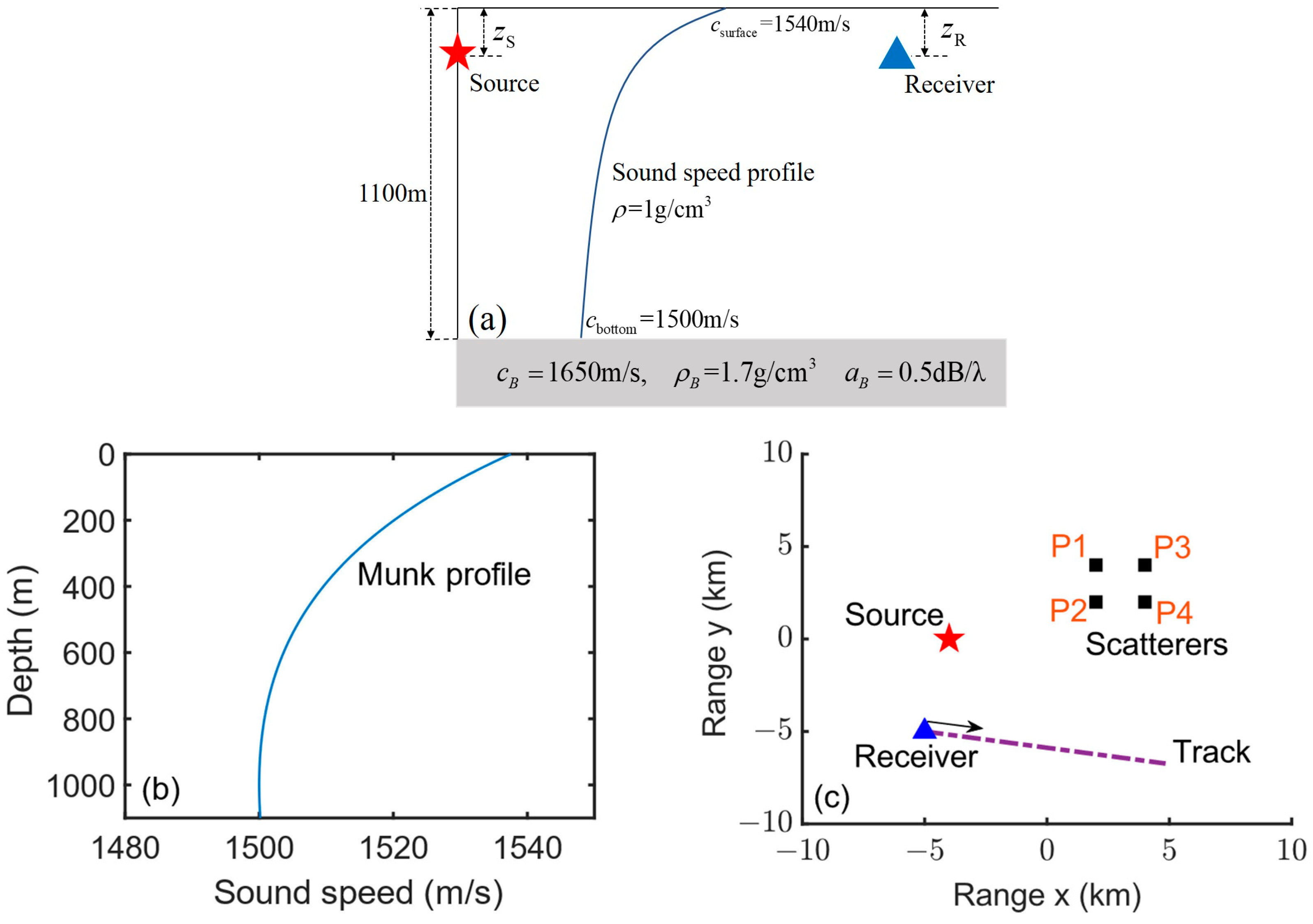
4.1. Simulation Environment and Parameters

In this section, simulations are used to verify the proposed method and the imaging results are compared with those of the BP method. The simulation environment is shown in Figure 6. The depth of the seafloor is 1100 m and the parameters of the infinite base in the single-layer seafloor model are shown in Figure 6a. The parameters of the source and the receiving array used in the simulation are consistent with the equipment parameters in the experiment. The source is a vertical transmitting array and the receiver is a horizontal towed array. The specific parameters of these two are detailed in

Table 1. The parameters of the source and the receiver in Figure 6a.

The Vertical Transmitting Array		The Horizontal Receiving Array		Frequency of the Signal
Number of Elements	Element Spacing	Number of Elements	Element Spacing	LFM
10	0.42 m	96	0.416 m	1700 Hz–1900 Hz

. A linear frequency modulation signal (LFM) is employed in the simulations, with a frequency ranging from 1700 Hz to 1900 Hz. The signal duration is 1 s and the sampling frequency is 16 kHz.

The parameters of the sound speed profile in Figure 6b are presented in

Table 2. The parameters of the Munk profile in Figure 6b.

$\mathbf{Munk} \mathbf{Profile} \mathit{c}\left(\mathit{z}\right)={\mathit{c}}_0\left\{1+\mathit{\xi }\left[{\mathit{e}}^{-\mathit{\varsigma }}-\left(1-\mathit{\varsigma }\right)\right]\right\}$$, \mathbf{Where} \mathit{\varsigma }=2\left(\mathit{z}-{\mathit{z}}_0\right)/{\mathit{B}}_{\mathit{W}}$
$\mathbf{The} \mathbf{Minimum} \mathbf{of} \mathbf{Sound} \mathbf{Speed} {\mathit{c}}_0$	$\mathbf{The} \mathbf{Depth} \mathbf{at} \mathbf{the} \mathbf{Minimum} \mathbf{of} \mathbf{Sound} \mathbf{Speed} {\mathit{z}}_0$	$\mathbf{The} \mathbf{Width} \mathbf{of} \mathbf{the} \mathbf{Waveguide} {\mathit{B}}_{\mathit{W}}$	The Extent of Deviation from the Minimum $\mathit{\xi }$
1500 m/s	1000 m	1000 m	0.57 × 10−2

. Additionally,

Table 3. The coordinates (x, y, z) for the source, the receiver, and the scatterers in Figure 6c.

The Center of the Source	The Initial Position of the Receiver	Scatterer P1	Scatterer P2	Scatterer P3	Scatterer P4
(−4 km, 0, 60 m)	(−5 km, −5 km, 60 m)	(2 km, 4 km, 1100 m)	(2 km, 2 km, 1100 m)	(4 km, 4 km, 1100 m)	(4 km, 2 km, 1100 m)

shows the coordinates of the source and the receiver, as well as those of the preset scatterers. The sound speed profile in the simulation is the Munk profile, which is obtained by using typical parameters. The minimum sound speed is 1500 m/s at a depth of 1000 m. In the top view of the imaging scene shown in Figure 6c, four scatterers are set within the range of 0 to 5 km in the x-axis direction and the range of 0 to 5 km in the y-axis direction. In the simulation, the position of the source is constant and a total of 50 receiving locations are set in the track.

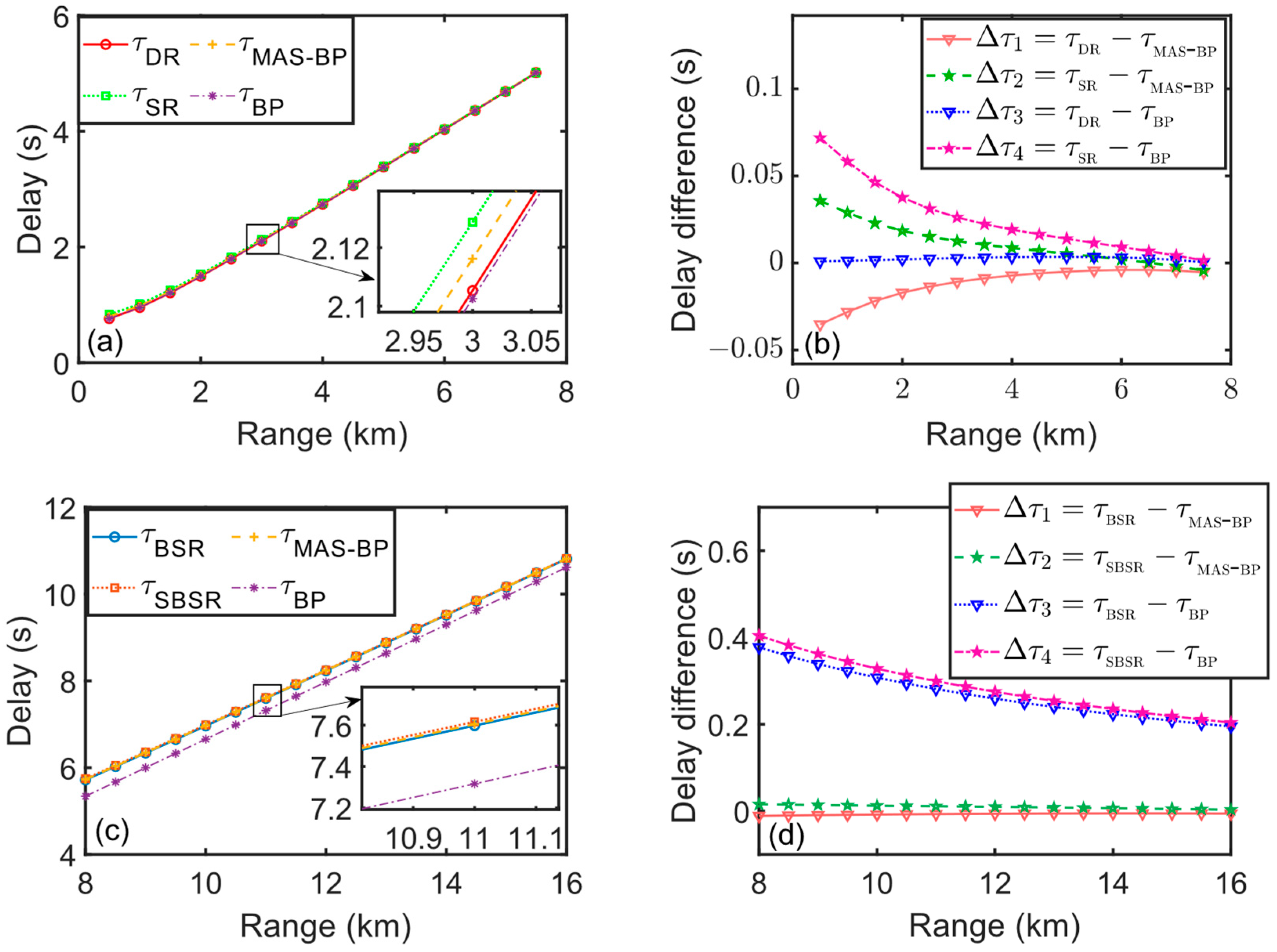
4.2. Comparison of Propagation Delay Values

The propagation time between the source and the grid calculated using the ray model, the delay calculated using the proposed MAS-BP method, and the delay calculated using the BP method are provided in Figure 7a,c. The difference between the delay calculated using the model and the results calculated using the two methods is shown in Figure 7b,d.

Figure 7a shows that the calculated delays ${\tau }_{\mathrm{MAS}-\mathrm{BP}}$ and ${\tau }_{\mathrm{BP}}$ are similar to the delays ${\tau }_{\mathrm{DR}}$ and ${\tau }_{\mathrm{SR}}$ in the direct zone, and the delay value increases monotonically with the range. In Figure 7b, since ${\tau }_{\mathrm{MAS}-\mathrm{BP}}$ is obtained from the average propagation time of the DR and SR, the difference between ${\tau }_{\mathrm{MAS}-\mathrm{BP}}$ and ${\tau }_{\mathrm{DR}}$, and that between ${\tau }_{\mathrm{MAS}-\mathrm{BP}}$ and ${\tau }_{\mathrm{SR}}$, are both within the range of 0 s to 0.05 s. The value of ${\tau }_{\mathrm{BP}}$ is close to that of ${\tau }_{\mathrm{DR}}$ and the difference is approximately 0; the difference between ${\tau }_{\mathrm{BP}}$ and ${\tau }_{\mathrm{SR}}$ is 0 s to 0.075 s. In Figure 7c,d, the value of ${\tau }_{\mathrm{MAS}-\mathrm{BP}}$ is similar to that of ${\tau }_{\mathrm{BSR}}$ and ${\tau }_{\mathrm{SBSR}}$ and the difference value is approximately 0. In contrast, the difference between ${\tau }_{\mathrm{BP}}$ and those two is more obvious, with a range from 0.2 s to 0.4 s.

Furthermore, the delay values from the source to the seafloor grid and then to the receiver calculated using the MAS-BP method and those calculated using the BP method are separately shown in Figure 8a,b. The difference between the calculation results of the two methods is shown in Figure 8c. Consistent with the theoretical analysis in Section 3, for the seafloor grid in the direct zone of the source and the receiver, the calculated results of the two methods are approximately equal. For the grid in the bottom bounce area of the source or the receiver, the difference between the two methods is in the range of 0.2 s to 0.4 s due to the absence of the DR and SR in the incident or scattering plane. Finally, for the distant grid, the BSR and SBSR are in the incident and scattering planes, without the DR and SR. The maximum value of the difference between the two methods is 0.8 s and the difference decreases with the range.

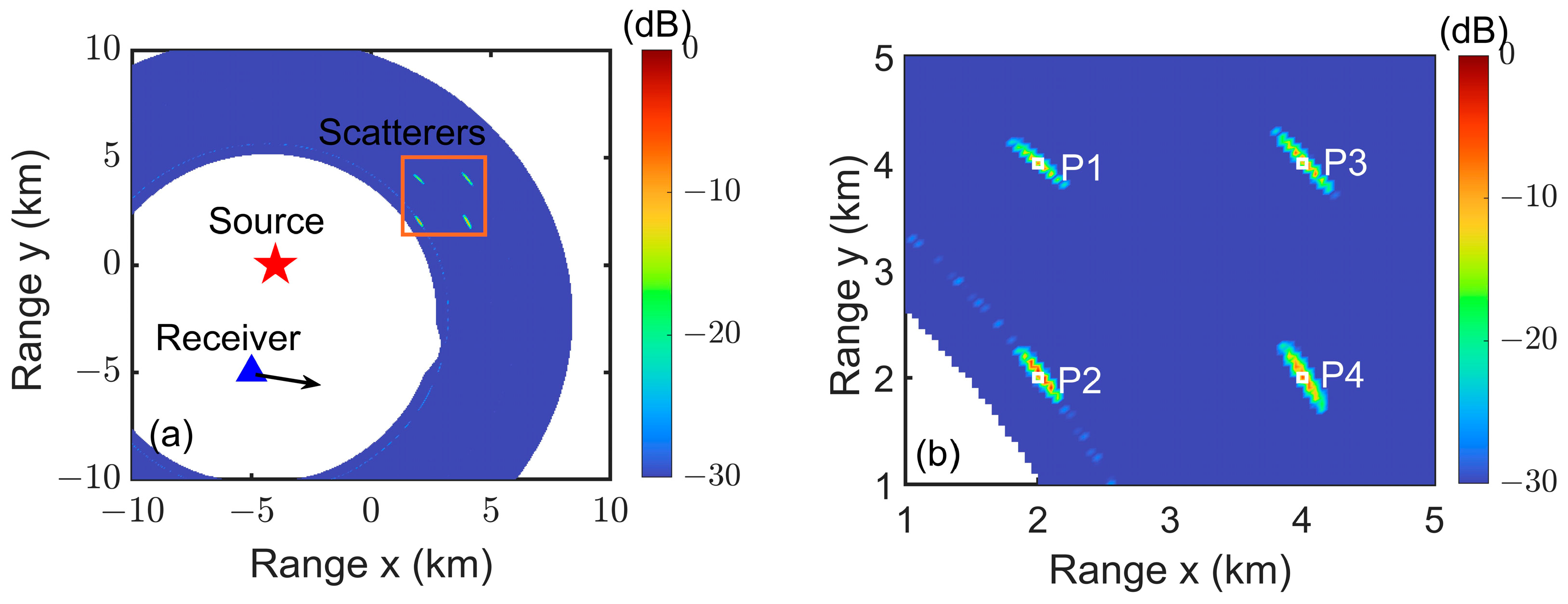
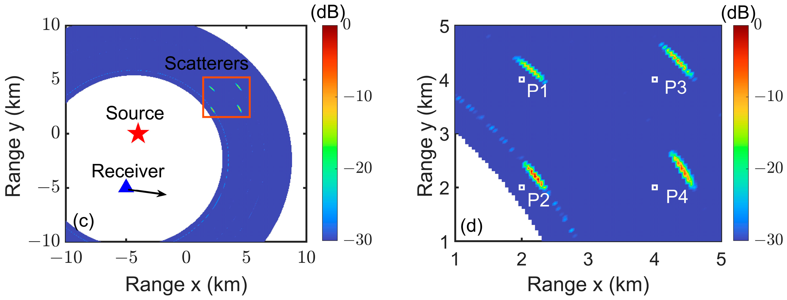
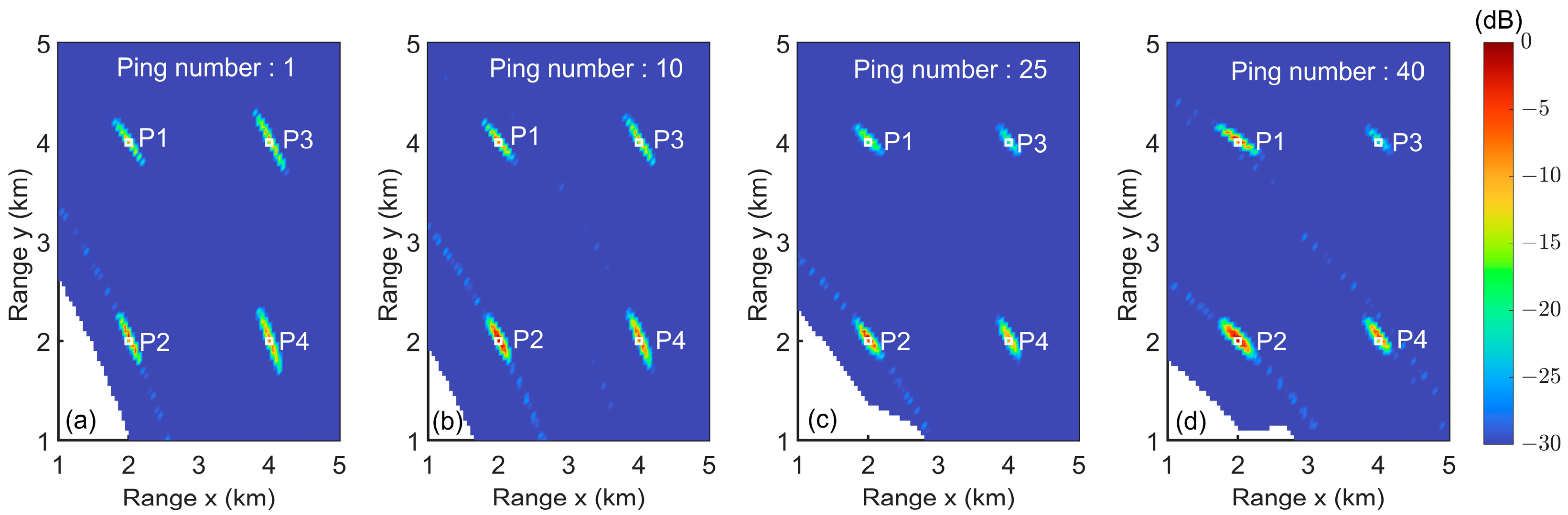
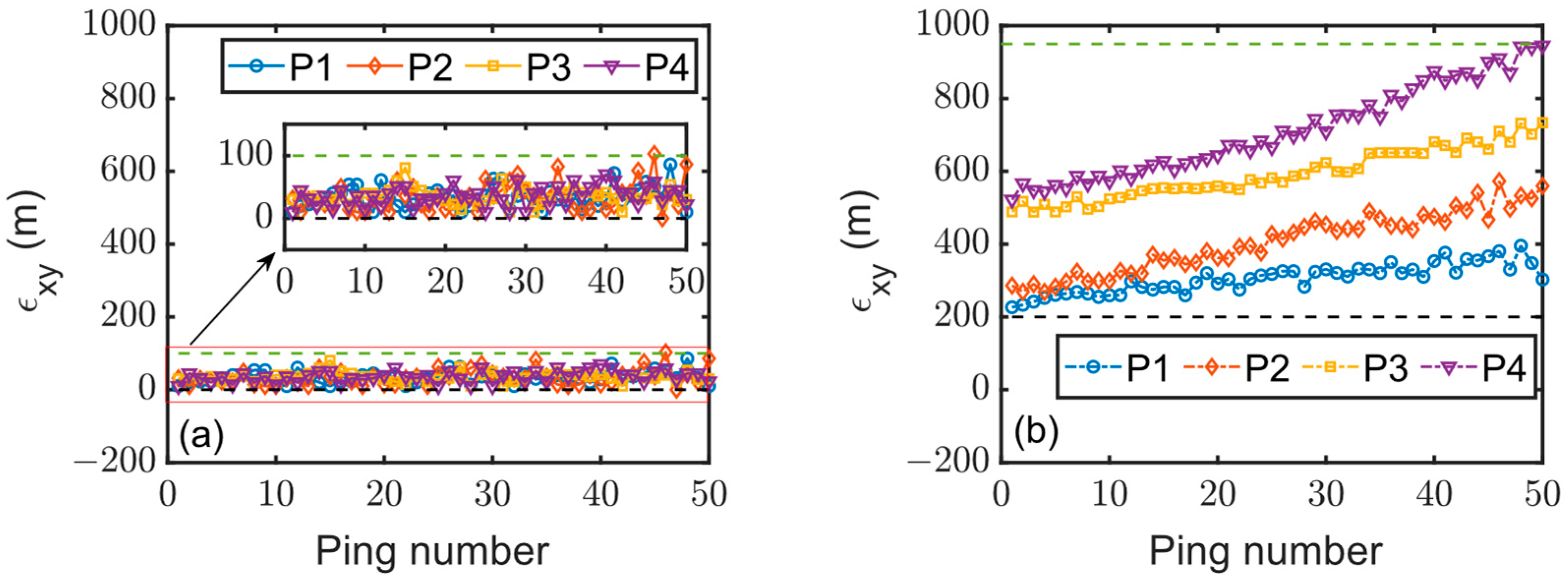
4.3. Imaging Results of Point Scatterers

In accordance with the results of the delay calculation in Section 4.2, the receiving array signals are further processed to generate a sound intensity image of the seafloor features. With the receiver at the starting position, the single-frame image obtained using the MAS-BP method and that obtained using the BP method are shown in Figure 9. The amplification of the rectangular frame areas in the images is shown in Figure 9b,d, where □ indicates the true position of the preset scatterer.

By comparing the result in Figure 9a with that in Figure 9c, it is obvious that there are four peaks in both images. The multipath structures are adopted to calculate the delay in the proposed method, and the positions of the peaks in Figure 9b are consistent with the positions of the scatterers. However, the calculated delay in the BP method is less than the actual propagation time. Consequently, the positions of the peaks are shifted to the upper right in Figure 9d, significantly deviating from the positions of the preset scatterers.

The images generated using the two methods at different receiving positions in the track are shown in Figure 10 and Figure 11. In Figure 10, the positions of the peaks in all four images are concordant with the positions of the scatterers, which verifies the effectiveness and feasibility of the MAS-BP method. Compared with the result in Figure 10, the positions of the peaks in Figure 11 change with the movement of the receiving array, and the deviation between the positions of the four peaks and the scatterers gradually increases.

To describe this deviation quantitatively, assuming that the position of the preset scatterer is $\left(x_{\mathrm{pre}},y_{\mathrm{pre}}\right)$ and the position of the peak in image is $\left(x_{\mathrm{peak}},y_{\mathrm{peak}}\right)$, the offset value ${\epsilon }_{xy}$ (unit: m) is defined as:

$${\epsilon }_{xy}=\sqrt{{\left(x_{\mathrm{peak}}-x_{\mathrm{pre}}\right)}^2+{\left(y_{\mathrm{peak}}-y_{\mathrm{pre}}\right)}^2}$$

(26)

The coordinates of the four peak points in Figure 10 and Figure 11 are extracted and the corresponding offsets are calculated using Equation (26).

Table 4. The four peak positions and offset values in Figure 10 (MAS-BP method), where the unit of coordinate (x, y) is (km, km).

The Coordinates (x, y) of the Scatterer		Ping No.1	Ping No.10	Ping No.25	Ping No.40
P1 (2, 4)	$\left(x_{\mathrm{peak}},y_{\mathrm{peak}}\right)$	(2.01, 4.00)	(2.01, 4.01)	(2.02, 4.03)	(2.02, 4.02)
	${\epsilon }_{xy}$ (m)	10	14.14	36.05	28.28
P2 (2, 2)	$\left(x_{\mathrm{peak}},y_{\mathrm{peak}}\right)$	(2.03, 2.01)	(2.01, 2.00)	(1.98, 2.06)	(1.99, 2.01)
	${\epsilon }_{xy}$ (m)	31.62	10	63.24	14.14
P3 (4, 4)	$\left(x_{\mathrm{peak}},y_{\mathrm{peak}}\right)$	(4.03, 4.00)	(4.00, 4.40)	(4.02, 4.02)	(3.99, 4.04)
	${\epsilon }_{xy}$ (m)	30	40	28.28	41.23
P4 (4, 2)	$\left(x_{\mathrm{peak}},y_{\mathrm{peak}}\right)$	(4.01, 2.00)	(4.01, 2.01)	(4.00, 2.01)	(4.00, 2.07)
	${\epsilon }_{xy}$ (m)	10	14.14	10	70.00

and

Table 5. The four peak positions and offset values in Figure 11 (BP method), where the unit of coordinate (x, y) is (km, km).

The Coordinates (x, y) of the Scatterer		Ping No.1	Ping No.10	Ping No.25	Ping No.40
P1 (2, 4)	$\left(x_{\mathrm{peak}},y_{\mathrm{peak}}\right)$	(2.17, 4.15)	(2.12, 4.23)	(2.07, 4.31)	(1.95, 4.35)
	${\epsilon }_{xy}$ (m)	226.71	259.42	317.81	353.55
P2 (2, 2)	$\left(x_{\mathrm{peak}},y_{\mathrm{peak}}\right)$	(2.23, 2.17)	(2.19, 2.23)	(2.08, 2.42)	(1.93, 2.47)
	${\epsilon }_{xy}$ (m)	286.00	298.33	427.55	475.18
P3 (4, 4)	$\left(x_{\mathrm{peak}},y_{\mathrm{peak}}\right)$	(4.36, 4.33)	(4.30, 4.43)	(4.24, 4.53)	(4.04, 4.68)
	${\epsilon }_{xy}$ (m)	488.36	524.31	581.81	681.17
P4 (4, 2)	$\left(x_{\mathrm{peak}},y_{\mathrm{peak}}\right)$	(4.42, 2.31)	(4.41, 2.40)	(4.31, 2.59)	(4.09, 2.87)
	${\epsilon }_{xy}$ (m)	522.02	572.80	666.48	874.64

present the positions and offset values of the peak points in Figure 10 and Figure 11, respectively. Along the x-axes and y-axes, the coordinates of each peak in Figure 10 closely align with those of the preset scatterers. Specifically, there is a maximum deviation of 30 m along the x-axes and 70m along the y-axis, corresponding to scatterer P4 in the image of Ping No.40. Accordingly, the offset value ${\epsilon }_{xy}$ is less than 100 m.

As shown in Table 5, the reflected eigenrays at a far distance are not considered in the BP method, resulting in a significant deviation between the positions of the peaks and those of the preset scatterers in Figure 11. The deviations of the peaks in the x-axes and y-axes exceed those presented in Table 4. Consequently, the offset value ${\epsilon }_{xy}$ varies from 226 m to 874 m.

Figure 12 shows the offset values of the four peaks in each frame image along the track. In Figure 12a, the imaging results of the four scatterers are minimally affected by the movement of the receiver, with each peak’s offset value remaining within 100 m across 50 receiving positions. Conversely, in Figure 12b, all four peak offsets exceed those in Figure 12a. Specifically, for scatterer P1, the offset ranges from 200 m to 400 m; for scatterer P2, it falls between 200 m and 500 m. Meanwhile, as scatterers P3 and P4 are further away from the source and receiver, the corresponding peaks give larger offset values ranging from 500 m to 950 m.

5. Application to Experimental Data

5.1. Experiment Description

An experiment was conducted near the northwest of the Xisha Islands in the South China Sea in June 2021. The source site and the track of the receiver, as well as the bathymetry of the experimental area, are shown in Figure 13a, where the depth data were obtained from the ETOPO1. The coordinate of the source is (111.562°E, 16.948°N). In addition, the origin is defined at the coordinates of (111.534°E, 17.005°N). The positive directions of the x-axes and y-axes correspond to east and north, respectively. The area in the center is relatively flat, with an average depth of approximately 1100 m, and the islands and reefs to the northwest are seen as significant scattering features for the imaging experiment.

The position of the source was fixed during the experiment and the receiving array moved close to the islands. Three tracks were set, with arrows indicating the heading of the receiving vessel. In Tracks 1 and 2, the receiving vessel followed a similar heading, while its position was situated to the west and east of the reefs, respectively. In Track 3, the receiving vessel was located on the eastern side of the reefs, with the heading directed towards the source.

The parameters of the transmitting array and the receiving array are shown in the simulations. The source depth was set to 60 m and an LFM signal with a frequency from 1700 Hz to 1900 Hz was transmitted, with a signal duration of 1 s. The depth of the receiving array was approximately 58 m and it was towed at a speed of 4 kn. In addition, the hydrophone sensitivity level was −142 dB.

Figure 13b shows the sound speed profile measured in the experiment, where the sound speed is constant within the depth of 0 to 50 m near the sea surface, and the value is approximately 1544.6 m/s. The sound velocity at the bottom of the sea is 1484 m/s.

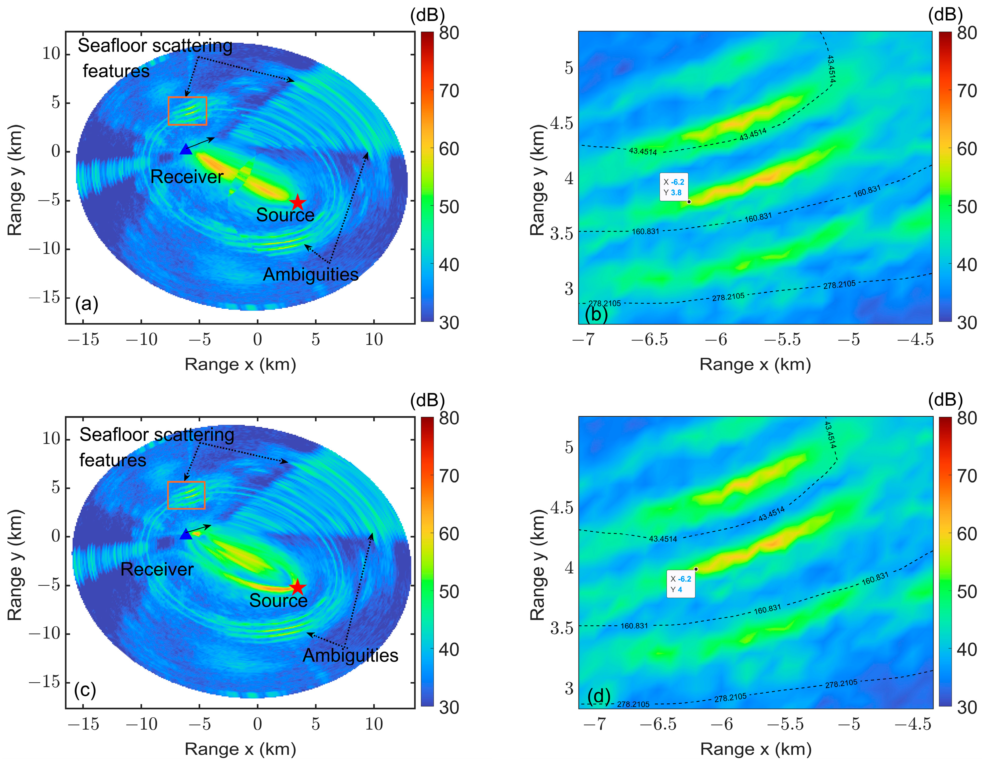
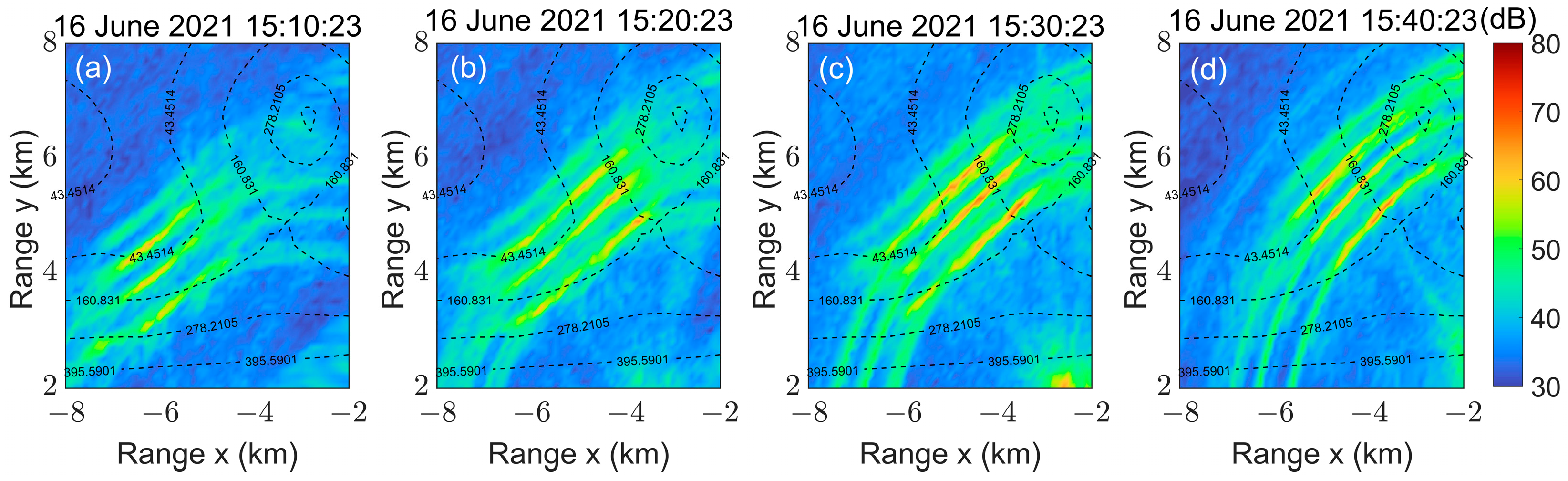
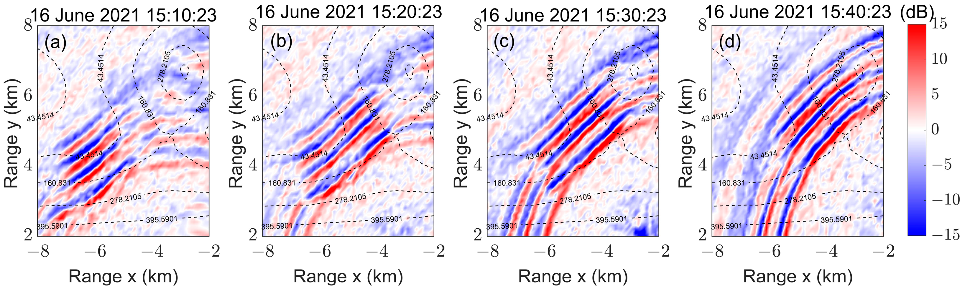
5.2. Experimental Results of Track 1

The experimental data are processed in this section. The received signals are processed using conventional beamforming and matching filtering, and then the beam outputs are projected to generate a seafloor image with the sound intensity amplitude.

Taking the experimental data collected at 15:00:23 on 16 June 2021 as an example, the data are processed using the MAS-BP method and the BP method, and the seafloor images are shown in Figure 14. Figure 14a,c present the diffuse reflection from the ocean environment and the prominent scattered echoes from the islands and reefs, as well as the background noise. During each transmission, the signals from the source–receiver plane are first received, and the region presents an elliptical area with a high amplitude of sound intensity. Subsequently, the diffuse reflection from the rough surface and the significant returns corresponding to the reefs arrive. The intensity of echoes decreases with distance due to propagation loss and absorption loss. As a result of the one-dimensionality of the horizontal array, the left–right ambiguities are almost symmetrically charted about the receiving array axis in the two images. In addition, the self-noise of the receiving ship is observed near the heading angle direction.

Figure 14b,d show the amplifications of the rectangular frame area in Figure 14a,c, respectively, with the corresponding ranges from −7 km to −4.5 km along the x-axis direction and from 3 km to 5 km along the y-axis direction. Bright stripes are observed in this area, which are the result of scattering caused by the island and reefs, and are correlated with the undulations of the terrain. To compare the positions of the reef features in the two images, a contour map of the experimental area is overlaid on the images. It can be seen that the structures of the stripes in Figure 14b,d are similar, but there are differences in specific locations. The two are essentially consistent along the x-axis direction, while the striated structures in the latter figure are shifted by 200 m compared to those of the former along the y-axis direction.

The explanation for the above phenomenon is as follows: Considering the positions of the source and the receiver, as well as the reefs in Figure 13a, the delay value calculated using the BP method is lower than the propagation time of the echoes. Consequently, the reef features in the seafloor image are shifted towards the northeast. Meanwhile, the receiving array is situated to the south of the islands and reefs, indicating minimal deviation of the reef features along the x-axis and significant deviation along the y-axis when projecting the beam outputs onto the seafloor grids. In contrast, the calculated delay is corrected using the proposed MAS-BP method, which is more closely matched to the travel time of the echoes. Therefore, the features of the reefs in the seafloor image are more consistent with the actual topography.

The imaging results obtained using the MAS-BP method and the BP method at different receiving times are shown in Figure 15 and Figure 16, respectively. Similarly, to the results shown in Figure 14, both figures present prominent striated structures within the northwestern area corresponding to the islands and reefs. Notably, the consistent appearance of striped structures indicates the presence of stable acoustic features or geological formations in the area, which provides important information for an analysis of seafloor sediment characteristics. With the movement of the receiving array, its position relative to the reefs varies significantly, resulting in the reception of echoes from different parts of the reefs. Accordingly, the areas of the reef features in the images change. Specifically, the area originally ranging from −8 km to −5 km along the x-axis and from 2 km to 6 km along the y-axis shifts to the area with a range from −6 km to −2 km along the x-axis and from 4 km to 7 km along the y-axis.

The difference in the sound intensity amplitude between Figure 15 and Figure 16 is illustrated in Figure 17. The red stripes indicate the locations of the reef features in the images generated using the MAS-BP method, while the blue stripes represent the locations of these features using the BP method. A comparative analysis reveals consistent results from both methods, with differences observed in the positions of the stripes. Similarly, to Figure 14, minimal variation in the position of the reef features is observed along the x-axis in Figure 15 and Figure 16; however, the positions of the features in Figure 16 shift from 200 m to 300 m along the y-axis.

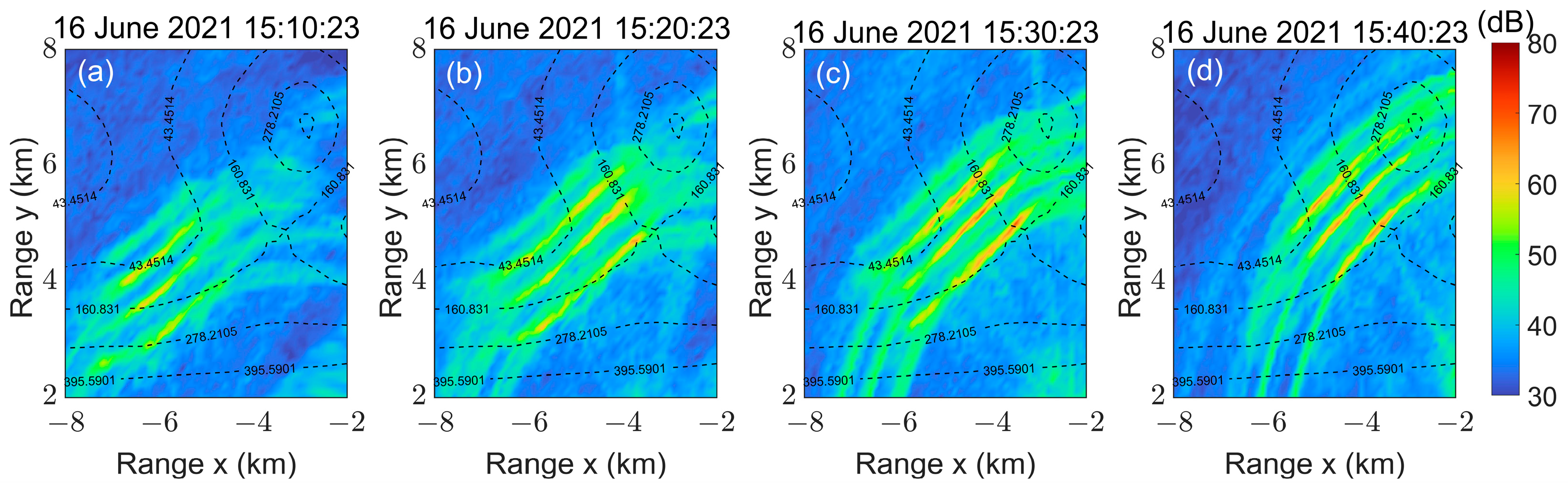
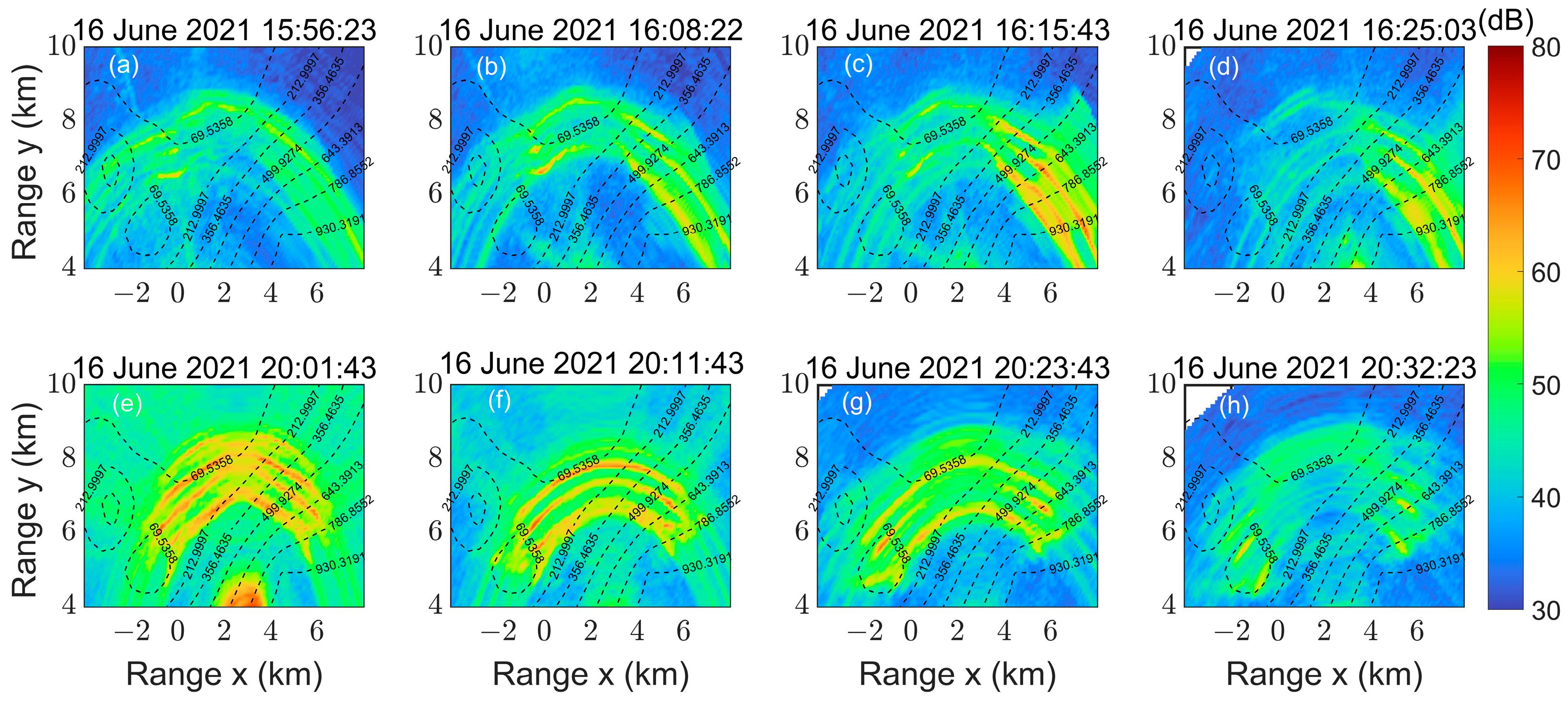
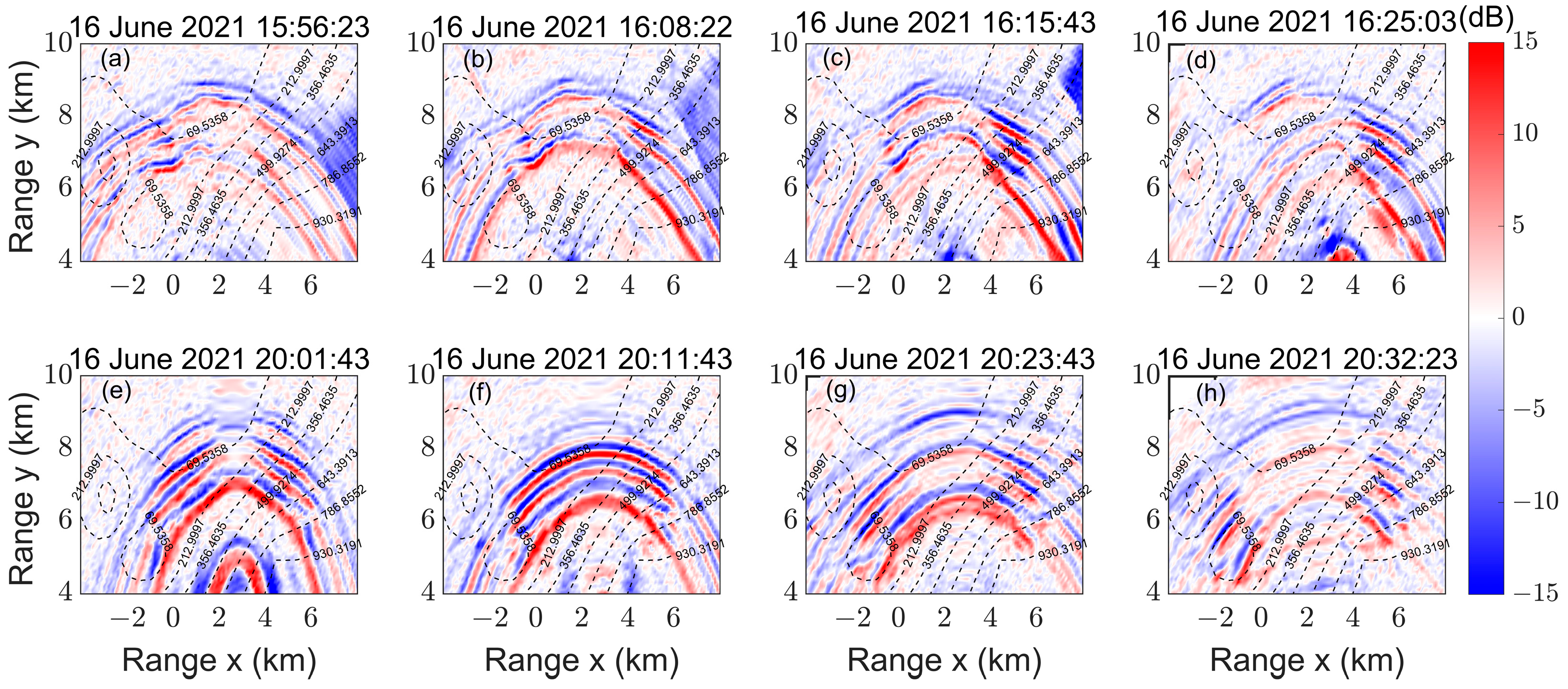
5.3. Experimental Results at Different Tracks

This section further presents the imaging results on Tracks 2 and 3. Figure 18 and Figure 19 depict the imaging outcomes obtained using the MAS-BP method and the BP method, respectively. In these two figures, subgraphs (a) to (d) correspond to Track 2, while subgraphs (e) to (h) correspond to Track 3.

Similarly, to the imaging results of Track 1, significant striped features corresponding to islands and reefs are also observed in those of Tracks 2 and 3. Since there are significant variations in the receiving positions, the area where the striped features appear is situated on the eastern side of the reefs. Specifically, it is within the region ranging from −2 km to 8 km along the x-axis and from 4 km to 9 km along the y-axis. Furthermore, despite the differing position and orientation of the receiving array in Tracks 2 and 3, the imaging results of these two tracks are consistent. This implies the presence of stable topographic features in the area. Combined with the contour lines, it is evident that the received signals predominantly come from the scattered signals on the eastern slope of the reefs. That is, the area is situated within a range of 4 km to 8 km along the x-axis and 4 km to 8 km along the y-axis.

For a specific track, changes in the position of the receiver result in corresponding shifts of the striped features in the image. However, the structure of the stripes remains unchanged, indicating that changes in position within a short time have a small impact on the imaging effect of the reefs. As the receiving array shifts, its position undergoes significant changes, resulting in the reception of scattered signals from different regions of the reefs. Consequently, the features observed in the image of each track correspond to a portion of the reefs rather than encompassing the entire area.

Figure 20 depicts the disparity in sound intensity between Figure 18 and Figure 19. Similarly, to the illustration in Figure 17, the structure of the red stripes (corresponding to Figure 18) and the blue stripes (corresponding to Figure 19) exhibits a high degree of similarity, albeit with differing spatial distributions. Specifically, the red stripes are situated closer to the reefs than the blue stripes. In the waveguide environment, the propagation delay calculated using the BP method is shorter than the actual propagation time of the seafloor grid. Therefore, when using projection to generate images, the amplitude at the grid will be projected to a further position. In other words, in the image generated using the BP method, the striped features of the reefs extend outward.

To quantitatively analyze the difference in the stripe positions, we extract the central positions of the stripes in images generated using the two methods separately, and then we calculate the distance between them. Due to the constraints of the experimental conditions, we lack an image of the true value of the sound intensity of the reef features. Therefore,

Table 6. The center coordinates (x, y) of the stripes in images generated using the two methods and the difference in distance between these two coordinates, where the unit of coordinate (x, y) is (km, km).

The Number of Data	The Center Coordinates of the Stripes for the MAS-BP Method	The Center Coordinates of the Stripes for the BP Method	The Distance Difference of Stripes (m)
Ping No.1	(−5.9, 4.2)	(−6.0, 4.3)	141.42
Ping No.2	(−5.3, 4.6)	(−5.2,4.8)	223.61
Ping No.3	(−5.0, 4.9)	(−5.1, 5.1)	223.61
Ping No.4	(−4.1, 5.6)	(−4.2, 5.8)	223.61
Ping No.5 *	(5.8, 6.0)	(5.9, 6.3)	316.23
Ping No.6 *	(5.8, 6.3)	(6.3, 6.3)	500.00
Ping No.7	(6.1, 6.0)	(6.3, 6.1)	223.61
Ping No.8	(6.6, 5.7)	(6.7, 5.8)	141.42
Ping No.9	(2.4, 7.7)	(2.7, 8.0)	424.26
Ping No.10	(1.8, 7.2)	(2.1, 7.6)	500.00
Ping No.11	(1.7, 7.2)	(1.6, 7.4)	223.61
Ping No.12	(1.6, 7.3)	(1.5, 7.7)	412.31

* Only the central location of the eastern stripes is calculated in Ping No.5 and Ping No.6.

only presents the relative distance difference in stripe positions of the two methods, with a total of 12-ping data points from three tracks.

The results in Table 6 indicate distinctions in the positions of stripes between the MAS-BP method and the BP method. Specifically, for Track 1, the stripe positions in the images generated using these two methods are concentrated and the deviation ranges from 140 m to 200 m. In Tracks 2 and 3, the slope in the eastern part of the reef is steeper, and there is a greater displacement of stripes in the BP method than in the MAS-BP method. The disparity in fringe distance between the two methods ranges from 140 m to 500 m.

By comparing the results of the two methods, it can be seen that the multipath structures should be taken into consideration when imaging the seafloor. In comparison with the BP method, the eigenrays are employed to reduce the deviation in the projection in the MAS-BP method, and the offset of the scattering features in the seafloor image is well corrected.

6. Summary and Conclusions

The propagation delay of echoes from the seafloor is influenced by the waveguide environment. In the case of a long distance, there is a significant deviation between the delay calculated using the BP method and the true value, which further results in deviations of the seafloor features in images of the sound intensity. To correct this deviation, a modified imaging method considering multipath structures is proposed in this paper.

In the proposed MAS-BP method, for short distances, the DR and SR are utilized to calculate the propagation delay, while for long distances, the BSR and SBSR are employed to calculate the propagation delay. Theoretical deduction demonstrates that the delay values calculated using the proposed method are similar to those calculated using the conventional method at short distances, leading to consistent results in seafloor imaging. At long distances, the proposed method provides more accurate calculations of the delay values than the conventional method, and it reduces the error in the projection and position deviation of the seafloor features in the images. Numerical simulations and experimental data results demonstrate the effectiveness and feasibility of the proposed method.

An accurate time delay is essential for imaging in practical applications. The proposed method offers a solution to mitigate the impact of the waveguide environment on underwater imaging. It enhances the detection and characterization of underwater features, including seafloor features and targets, which are crucial for marine exploration and environmental monitoring.

However, some limitations affect the application of this method. Firstly, the imaging range is influenced by both the distance and waveguide environment. The method becomes ineffective when the distance between the seafloor grid and the source or receiver exceeds the operational range of the eigenrays used, such as the SBSR and BSR. Secondly, this method is not suitable for environments with significant changes in seabed topography or strong ocean phenomena such as internal waves and fronts. These phenomena can lead to changes in the sound speed profile and thus affect the structure of the eigenrays. Considering these conditions, we initially propose the following solution: To address imaging at longer distances, the time delay can be calculated using multiple reflected eigenrays to extend the imaging range. For the second case, sound field models may replace the current method. By integrating accurate environmental parameter information, such as the seabed topography and sound velocity profile with distance variation, the sound field model enables a more precise calculation of the propagation time and the structure of the eigenrays.

There are many improvements to be made in future research. For example, this research is applicable to seafloor imaging and could also be utilized for target imaging in ocean environments. Considering the variations in seabed topography and the changes in sound speed resulting from significant oceanic phenomena, it is valuable to explore methods for achieving seabed or target imaging in complex environments. Meanwhile, high-resolution beamforming techniques can also be employed to enhance the imaging resolution with this approach. Furthermore, to fulfill real-time requirements, the grid division and projection with this approach can be used in parallel to enhance processing speed.

References

1. Makris, N.C.; Jagannathan, S.; Ignisca, A. Ocean Acoustic Waveguide Remote Sensing: Visualizing Life Around Seamounts. Oceanography 2010, 23, 204–205. [Google Scholar] [CrossRef]
2. Jagannathan, S.; Bertsatos, I.; Symonds, D.T.; Chen, T.; Nia, H.T.; Jain, A.D.; Andrews, M.J.; Gong, Z.; Nero, R.W.; Ngor, L.; et al. Ocean Acoustic Waveguide Remote Sensing (OAWRS) of marine ecosystems. Mar. Ecol. Prog. Ser. 2009, 395, 137–160. [Google Scholar] [CrossRef]
3. Makris, N.C.; Avelino, L.Z.; Menis, R. Deterministic Reverberation from Ocean Ridges. J. Acoust. Soc. Am. 1995, 97, 3547–3574. [Google Scholar] [CrossRef]
4. Makris, N.C.; Berkson, J.M. Long-Range Backscatter from the Mid-Atlantic Ridge. J. Acoust. Soc. Am. 1994, 95, 1865–1881. [Google Scholar] [CrossRef]
5. Zheng, Y.; Ping, X.; Li, L.; Wang, D. Maximum Likelihood Deconvolution of Beamforming Images with Signal-Dependent Speckle Fluctuations. Remote Sens. 2024, 16, 1506. [Google Scholar] [CrossRef]
6. Makris, N.C.; Ratilal, P.; Jagannathan, S.; Gong, Z.; Andrews, M.; Bertsatos, I.; Godø, O.; Nero, R.; Jech, J. Critical Population Density Triggers Rapid Formation of Vast Oceanic Fish Shoals. Science 2009, 323, 1734–1737. [Google Scholar] [CrossRef] [PubMed]
7. Makris, N.C.; Ratilal, P.; Symonds, D.T.; Jagannathan, S.; Lee, S.; Nero, R.W. Fish population and behavior revealed by instantaneous continental shelf-scale imaging. Science 2006, 311, 660–663. [Google Scholar] [CrossRef]
8. Duane, D.; Godø, O.R.; Makris, N.C. Quantification of Wide-Area Norwegian Spring-Spawning Herring Population Density with Ocean Acoustic Waveguide Remote Sensing (OAWRS). Remote Sens. 2021, 13, 4546. [Google Scholar] [CrossRef]
9. Eleftherios, K.; Ratilal, P.; Makris, N.C. Optimal Automatic Wide-Area Discrimination of Fish Shoals from Seafloor Geology with Multi-Spectral Ocean Acoustic Waveguide Remote Sensing in the Gulf of Maine. Remote Sens. 2023, 15, 437. [Google Scholar] [CrossRef]
10. Gong, Z.; Andrews, M.; Jagannathan, S.; Patel, R.; Jech, J.M.; Makris, N.C.; Ratilal, P. Low-Frequency Target Strength and Abundance of Shoaling Atlantic Herring (Clupea harengus) in the Gulf of Maine during the Ocean Acoustic Waveguide Remote Sensing 2006 Experiment. J. Acoust. Soc. Am. 2010, 127, 104–123. [Google Scholar] [CrossRef]
11. Lee, W.J.; Tang, D.; Stanton, T.K.; Thorsos, E.I. Macroscopic Observations of Diel Fish Movements around a Shallow Water Artificial Reef Using a Mid-Frequency Horizontal-Looking Sonar. J. Acoust. Soc. Am. 2018, 144, 1424–1434. [Google Scholar] [CrossRef]
12. Yi, D.H.; Gong, Z.; Jech, J.M.; Ratilal, P.; Makris, N.C. Instantaneous 3D Continental-Shelf Scale Imaging of Oceanic Fish by Multi-Spectral Resonance Sensing Reveals Group Behavior during Spawning Migration. Remote Sens. 2018, 10, 108. [Google Scholar] [CrossRef]
13. Yi, D.H.; Makris, N.C. Feasibility of Acoustic Remote Sensing of Large Herring Shoals and Seafloor by Baleen Whales. Remote Sens. 2016, 8, 693. [Google Scholar] [CrossRef]
14. Wang, D.; Huang, W.; Garcia, H.; Ratilal, P. Vocalization Source Level Distributions and Pulse Compression Gains of Diverse Baleen Whale Species in the Gulf of Maine. Remote Sens. 2016, 8, 881. [Google Scholar] [CrossRef]
15. Preston, J.R.; Akal, T.; Berkson, J. Analysis of Backscattering Data in the Tyrrhenian Sea. J. Acoust. Soc. Am. 1990, 87, 119–134. [Google Scholar] [CrossRef]
16. Makris, N.C.; Chia, C.S.; Fialkowski, L.T. The Bi-Azimuthal Scattering Distribution of an Abyssal Hill. J. Acoust. Soc. Am. 1999, 106, 2491–2512. [Google Scholar] [CrossRef]
17. Chia, C.S.; Makris, N.C.; Fialkowski, L.T. A Comparison of Bistatic Scattering from Two Geologically Distinct Abyssal Hills. J. Acoust. Soc. Am. 2000, 108, 2053–2070. [Google Scholar] [CrossRef]
18. Yang, J.; Tang, D.; Hefner, B.T.; Williams, K.L.; Preston, J.R. Overview of Midfrequency Reverberation Data Acquired During the Target and Reverberation Experiment 2013. IEEE J. Oceanic Eng. 2018, 43, 563–585. [Google Scholar] [CrossRef]
19. Jung, Y.; Lee, K. Observation of the Relationship between Ocean Bathymetry and Acoustic Bearing-Time Record Patterns Acquired during a Reverberation Experiment in the Southwestern Continental Margin of the Ulleung Basin, Korea. J. Mar. Sci. Eng. 2021, 9, 1259. [Google Scholar] [CrossRef]
20. Ratilal, P.; Lai, Y.; Symonds, D.T.; Ruhlmann, L.A.; Preston, J.R.; Scheer, E.K.; Garr, M.T.; Holland, C.W.; Goff, J.A.; Makris, N.C. Long Range Acoustic Imaging of the Continental Shelf Environment: The Acoustic Clutter Reconnaissance Experiment 2001. J. Acoust. Soc. Am. 2005, 117, 1977–1998. [Google Scholar] [CrossRef]
21. Galinde, A.; Donabed, N.; Andrews, M.; Lee, S.; Makris, N.C.; Ratilal, P. Range-Dependent Waveguide Scattering Model Calibrated for Bottom Reverberation in a Continental Shelf Environment. J. Acoust. Soc. Am. 2008, 123, 1270–1281. [Google Scholar] [CrossRef]
22. Jagannathan, S.; Küsel, E.T.; Ratilal, P.; Makris, N.C. Scattering from Extended Targets in Range-Dependent Fluctuating Ocean-Waveguides with Clutter from Theory and Experiments. J. Acoust. Soc. Am. 2012, 132, 680–693. [Google Scholar] [CrossRef]
23. Preston, J.R.; Ellis, D.D. Extracting Bottom Information from Towed-Array Reverberation Data: Part I: Measurement Methodology. J. Mar. Syst. 2009, 78 (Suppl. C), S359–S371. [Google Scholar] [CrossRef]
24. Preston, J.R. Extracting bottom information from towed-array reverberation data. Part II: Extraction procedure and modelling methodology. J. Mar. Syst. 2009, 78 (Suppl. S), S372–S381. [Google Scholar] [CrossRef]
25. Ellis, D.D.; Yang, J.; Preston, J.R.; Pecknold, S. A Normal Mode Reverberation and Target Echo Model to Interpret Towed Array Data in the Target and Reverberation Experiments. IEEE J. Ocean. Eng. 2017, 42, 344–361. [Google Scholar] [CrossRef]
26. Prior, M.K. A Scatterer Map for the Malta Plateau. IEEE J. Ocean. Eng. 2005, 30, 676–690. [Google Scholar] [CrossRef]
27. Preston, J.R.; Abraham, D.A. Statistical Analysis of Multistatic Echoes from a Shipwreck in the Malta Plateau. IEEE J. Ocean. Eng. 2015, 40, 643–656. [Google Scholar] [CrossRef]
28. Holland, C. Mapping seabed variability: Rapid surveying of coastal regions. J. Acoust. Soc. Am. 2006, 119, 1373–1387. [Google Scholar] [CrossRef]
29. Zhang, X.; Yang, P.; Tan, C.; Ying, W. BP Algorithm for the Multireceiver SAS. IET Radar Sonar Navig. 2019, 13, 830–838. [Google Scholar] [CrossRef]
30. Ellis, D.D.; Crowe, D.V. Bistatic reverberation calculations using a three-dimensional scattering function. J. Acoust. Soc. Am. 1991, 89, 2207–2214. [Google Scholar] [CrossRef]
31. Wang, L.; Qin, J.; Fu, D.; Li, Z.; Liu, J.; Weng, J. Bottom reverberation for large receiving depth in deep water. Acta Phys. Sin. 2019, 68, 134303. [Google Scholar] [CrossRef]
Figure 1. Acoustic imaging scene of bistatic sonar. (a) Side view. (b) Top view.
Remotesensing 16 02586 g001
Figure 2. The multipath structures from the source to the seafloor scatterer and then to the receiver. (a) SR/DR-SR/DR. (b) SR/DR-BSR/SBSR. (c) BSR/SBSR-SR/DR. (d) BSR/SBSR-BSR/SBSR.
Remotesensing 16 02586 g002
Figure 3. The eigenray path, the exit angle of the eigenray at the source, and the grazing angle of the eigenray at the scatterer. (a) Eigenray path in the direct zone. (b) The grazing angle varies with range in the direct zone. (c) Eigenray path in the bottom bounce zone. (d) The grazing angle varies with range in the bottom bounce zone.
Remotesensing 16 02586 g003
Figure 4. Projection of the beam output onto the image of seafloor features.
Remotesensing 16 02586 g004
Figure 5. Flow chart of the MAS-BP method.
Remotesensing 16 02586 g005
Figure 6. Simulation environment. (a) The parameters of the simulation environment. (b) The Munk profile employed in the simulation. (c) Top view of the imaging scene.
Remotesensing 16 02586 g006
Figure 7. The delay value varies with range. (a) The delay value in the direct zone. (b) The delay difference in the direct zone. (c) The delay value in the bottom bounce zone. (d) The delay difference in the bottom bounce zone.
Remotesensing 16 02586 g007
Figure 8. The delay calculated using the MAS-BP method and the BP method. (a) The MAS-BP method. (b) The BP method. (c) The delay difference between the MAS-BP method and the BP method.
Remotesensing 16 02586 g008
Figure 9. Imaging results of scatterers generated using the MAS-BP method and the BP method. (a) The MAS-BP method. (b) Amplification of rectangular frame area in Figure 9a. (c) The BP method. (d) Amplification of rectangular frame area in Figure 9c.
Remotesensing 16 02586 g009aRemotesensing 16 02586 g009b
Figure 10. Images generated using the MAS-BP method at four receiving positions. (a) Position No.1. (b) Position No.10. (c) Position No.25. (d) Position No.40.
Remotesensing 16 02586 g010
Figure 11. Images generated using the BP method at four receiving positions. (a) Position No.1. (b) Position No.10. (c) Position No.25. (d) Position No.40.
Remotesensing 16 02586 g011
Figure 12. The peak offset values of four scatterers in each image in the track. (a) The results of the MAS-BP method. (b) The results of the BP method.
Remotesensing 16 02586 g012
Figure 13. Experimental environment. (a) Bathymetry of the experimental area. (b) The measured sound speed profile.
Remotesensing 16 02586 g013
Figure 14. Imaging results of experimental data processed using the MAS-BP method and the BP method. (a) The image generated using the MAS-BP method. (b) Amplification of rectangular frame area in Figure 14a. (c) The image generated using the BP method. (d) Amplification of rectangular frame area in Figure 14c.
Remotesensing 16 02586 g014
Figure 15. Imaging results of experimental data processed using the MAS-BP method at different receiving times. (a) 16 June 2021 15:10:23. (b) 16 June 2021 15:20:23. (c) 16 June 2021 15:30:23. (d) 16 June 2021 15:40:23.
Remotesensing 16 02586 g015
Figure 16. Imaging results of experimental data processed using the BP method at different receiving times. (a) 16 June 2021 15:10:23. (b) 16 June 2021 15:20:23. (c) 16 June 2021 15:30:23. (d) 16 June 2021 15:40:23.
Remotesensing 16 02586 g016
Figure 17. The difference between the amplitude of sound intensity in Figure 15 and that in Figure 16 at different receiving times. (a) 16 June 2021 15:10:23. (b) 16 June 2021 15:20:23. (c) 16 June 2021 15:30:23. (d) 16 June 2021 15:40:23.
Remotesensing 16 02586 g017
Figure 18. Imaging results of experimental data processed using the MAS-BP method, where (ad) correspond to Track 2 and (eh) correspond to Track 3. (a) 16 June 2021 15:56:23. (b) 16 June 2021 16:08:22. (c) 16 June 2021 16:15:43. (d) 16 June 2021 16:25:03. (e) 16 June 2021 20:01:43. (f) 16 June 2021 20:11:43. (g) 16 June 2021 20:23:43. (h) 16 June 2021 20:32:23.
Remotesensing 16 02586 g018
Figure 19. Imaging results of experimental data processed using the BP method, where (ad) correspond to Track 2 and (eh) correspond to Track 3. (a) 16 June 2021 15:56:23. (b) 16 June 2021 16:08:22. (c) 16 June 2021 16:15:43. (d) 16 June 2021 16:25:03. (e) 16 June 2021 20:01:43. (f) 16 June 2021 20:11:43. (g) 16 June 2021 20:23:43. (h) 16 June 2021 20:32:23.
Remotesensing 16 02586 g019
Figure 20. The difference between the amplitude of sound intensity in Figure 18 and that in Figure 19, where (ad) correspond to Track 2 and (eh) correspond to Track 3. (a) 16 June 2021 15:56:23. (b) 16 June 2021 16:08:22. (c) 16 June 2021 16:15:43. (d) 16 June 2021 16:25:03. (e) 16 June 2021 20:01:43. (f) 16 June 2021 20:11:43. (g) 16 June 2021 20:23:43. (h) 16 June 2021 20:32:23.
Remotesensing 16 02586 g020