Spatial Distribution and Variation in Debris Cover and Flow Velocities of Glaciers during 1989–2022 in Tomur Peak Region, Tianshan Mountains

Abstract

In this study, we utilized a feature optimization method combining texture and topographical factors with the random forest (RF) approach to identify changes in the extent of the debris cover around the Tianshan Tomur Peak between 1989 and 2022. Based on Sentinel-1 image data, we extracted glacier flow velocities using an offset tracking method and conducted a long-term analysis of flow velocities in combination with existing datasets. The debris identification results for 2022 showed that the debris-covered area in the study region was 409.2 km², constituting 22.8% of the total glacier area. Over 34 years, the area of debris cover expanded by 69.4 km², reflecting a growth rate of 20.0%. Analysis revealed that glaciers in the Tomur Peak area have been decelerating at an overall rate of −4.0% per decade, with the complexity of the glacier bed environment and the instability of the glacier’s internal structure contributing to significant seasonal and interannual variability in the movement speeds of individual glaciers.

1. Introduction

According to the Sixth Assessment Report by the Intergovernmental Panel on Climate Change (IPCC), there is an increasing global rate of mass loss from mountain glaciers, with human-induced climate warming identified as the primary cause of glacier mass depletion [1]. Local glacial climate (temperature, precipitation, snowfall, etc.) along with non-climatic factors (topography, size, glacial ice temperature, etc.) result in significant spatial variability in glacier changes [1,2,3]. Located primarily in the ablation zones of glaciers, debris cover is another significant non-climatic factor influencing glacier dynamics. Thin layers of debris reduce the surface albedo of glaciers, increasing radiation absorption and thereby accelerating the melting of the underlying ice; conversely, thick debris layers act as an insulating barrier, inhibiting the melting of the ice below [4,5,6,7].

With the intensification of changes to glaciers, many debris-covered glaciers are experiencing varying degrees of expansion in their debris-covered areas [8,9,10,11,12,13], gradually highlighting the role of debris in glacier melting and movement processes. The spectral reflectance characteristics of debris, similar to those of surrounding rocks and moraine material, present a “different object with same spectrum” phenomenon, leading to the ineffectiveness of conventional glacier information extraction methods in identifying debris cover. Addressing this challenge involves considering various factors (topography, texture, surface temperature, etc.) and integrating multi-source data, becoming the primary means of enhancing the accuracy of debris cover identification [14,15,16,17]. Remote sensing spectral information of mountain glaciers exhibits high variability temporally and spatially, and debris cover characteristics like the distribution slope and surface temperature range vary as well. Machine learning methods significantly enhance work efficiency by learning target patterns and features from large datasets and automatically selecting appropriate thresholds for image classification. Neural networks, random forests, and support vector machines are machine learning methods widely applied in debris cover identification studies [11,16,17,18,19].

Glacier flow velocity serves as a key indicator reflecting glacier mass redistribution. Primarily controlled by glacier thickness, a reduction in thickness due to mass loss leads to decreased glacier velocity [20,21]. The presence of debris cover slows glacier retreat and thinning, substantially preserving terminus activity. Debris moves with the underlying ice, with its displacement speed essentially equivalent to the glacier’s surface speed. Debris movement on the ice surface and local thickness changes are mainly governed by the glacier’s horizontal velocity field [22,23,24]. The accumulation of moraine material and the development of supraglacial ponds and terminal moraine lakes make debris-covered glaciers more prone to disasters like glacial debris-flows and moraine-dammed lake outbursts [25,26,27,28]. Glacier movement is closely related to glacial disasters, and its monitoring provides crucial evidence for studying and predicting such disasters [29,30,31].

Glacier flow velocity extraction methods are classified into optical and radar remote sensing techniques. In optical remote sensing, cloud cover severely impacts image quality. For instance, in mid-latitude regions such as the Tianshan Mountains, frequent cloud cover above glaciers often results in significant data gaps [32]. The Synthetic Aperture Radar (SAR) imaging system demonstrates advantages in all-weather operation and cloud penetration [33]. Glacier velocity estimation methods using SAR data are divided into differential interferometric synthetic aperture radar (DInSAR) and offset-tracking [34]. Although DInSAR provides considerable accuracy in estimating velocities, decorrelation phenomena impede its further development and application. Conversely, offset-tracking does not face decorrelation issues and is minimally impacted by terrain undulations with short spatial baselines, suiting the mountainous terrain of debris-covered glaciers. Satellite-borne SAR systems operate in varying bands, with L, C, and X bands suitable for estimating debris-covered glacier flow velocities using offset-tracking [32,35,36,37].

The Central Tianshan Tomur Peak Region hosts China’s largest concentration of debris-covered glaciers [38]. It is relatively complicated to correctly identify debris-covered glaciers based on remote sensing data, due to the “different object with same spectrum” issue. This limitation may be addressed by employing a feature optimization method that combines texture and topographical factors with the random forest approach. To achieve this, we used Landsat satellite data to identify changes in the extent of debris cover on glaciers around the Tomur Peak from 1989 to 2022. The study estimated the surface flow velocities of Tomur-type glaciers within the study area for 2020–2022, focusing on identified debris-covered areas, using the offset-tracking method. This analysis was augmented by combining glacier flow velocity data from 1989–2020 from the ITS_LIVE dataset and the Sentinel-1 glacier motion velocity dataset [39], to conduct a long-term analysis of surface flow velocities of debris-covered glaciers within the study area.

2. Study Area

Located at the trijunction of Kazakhstan, Kyrgyzstan, and China (41°10′N–42°40′N, 79°20′E–80°55′E), the Tomur-Khan Tengri Mountain Range is depicted in Figure 1. Around 60% of this region’s land exceeds 4000 m in elevation, and its highest point, Tomur Peak, ascends to 7443.8 m. The glaciers in the Tomur Peak region are primarily dendritic large valley glaciers, characterized by their long, narrow tongues, extensive supraglacial debris cover, and well-developed thermokarst features. These glaciers can be referred to as “Tomur-type” glaciers. This study focused on Tomur-type glaciers in the Tomur Peak region, specifically those with an area greater than 40 km².

The Tomur Peak Region features a temperate continental climate, influenced by prevailing westerlies, with abundant precipitation mainly concentrated in the glacier melt season, accounting for 70% of the annual total [40,41]. The extensive elevation range of the glaciers and abundant material supply in the study area contribute to relatively high glacier velocities. Glacial processes, including erosion, transport, and deposition, are pronounced, fostering conditions for extensive development of debris cover. The melt season of glaciers in the Tomur Peak Region is from May to September. Debris cover serves as an “insulating barrier”, mitigating glacial mass loss and curtailing glacier retreat and thickness reduction, thereby preserving glacier terminus activity to some extent.

3. Data and Methods

The experimental workflow of this study is shown in Figure 2. We utilized a feature optimization random forest method, combining texture and topographical factors, to identify the extent of debris cover around Tomur Peak in Central Tianshan. The method involved extracting and optimizing spectral, topographical, and texture features. Given the significant impact of cloud cover on optical image quality, we conducted flow velocity estimation from 2021 to 2022 using the SAR-based offset-tracking method. Debris distribution enhances glacier surface features, offering favorable conditions for remote sensing estimation of glacier velocities [42]. Glacier velocity estimations within debris-covered areas tend to be more stable and accurate [43]. To ensure the reliability of our conclusions, the analysis of glacier velocity was limited to the debris-covered areas identified in 2007.

3.1. Data Sources

3.1.1. Satellite Data

Landsat image data were obtained from the USGS Earth Explorer website (http://earthexplorer.usgs.gov/, accessed on 1 July 2024), as detailed in

Table 1. List of Landsat scenes used to map supra-glacial debris.

Path-Row	Date	LANDSAT_SCENE_ID	Sensor	Cloud Cover (%)
147-031	22 August 1989	LT51470311989234ISP00	TM	3
147-031	10 September 1996	LT51470311996254ISP00	TM	3
147-031	24 August 2007	LT51470312007236IKR00	TM	10
147-031	1 September 2016	LC81470312016245LGN01	OLI	6.79
147-031	13 July 2022	LE71470312022194NPA00	ETM+	33
147-031	24 July 2022	LC91470312022205LGN01	OLI	26.48

. Cloud-covered images were excluded, and selections were made from the latter part of the glacier melt season to reduce the impact of seasonal snow cover. For 2022, two images were combined to address cloud cover. Atmospheric correction was applied to all Landsat images, converting the original brightness values (digital numbers, DNs) to surface reflectance, to mitigate sensor differences and variations in observational conditions.

We acquired Sentinel-1A data from the National Aeronautics and Space Administration (NASA)’s Alaska Satellite Facility. For glacier flow velocity estimation, this study utilized 49 single look complex (SLC) images, collected by Sentinel-1A from 2019 to 2022. The images’ orbit and frame numbers were 158 and 132, respectively, with temporal baselines of 24 or 36 days.

Table 2. Sentienl-1A SAR offset-tracking data pairs used in this study.

No.	Date-1_Date-2	No.	Date-1_Date-2
1	31 December 2020_5 February 2021	13	26 December 2021_31 January 2022
2	5 February 2021_1 March 2021	14	31 January 2022_24 February 2022
3	1 March 2021_25 March 2021	15	24 February 2022_1 April 2022
4	25 March 2021_30 April 2021	16	1 April 2022_7 May 2022
5	30 April 2021_5 June 2021	17	7 May 2022_31 May 2022
6	5 June 2021_29 June 2021	18	31 May 2022_24 June 2022
7	29 June 2021_4 August 2021	19	24 June 2022_30 July 2022
8	4 August 2021_28 August 2021	20	30 July 2022_4 September 2022
9	28 August 2021_3 October 2021	21	4 September 2022_28 September 2022
10	3 October 2021_27 October 2021	22	28 September 2022_3 November 2022
11	27 October 2021_2 December 2021	23	3 November 2022_9 December 2022
12	2 December 2021_26 December 2021	24	9 December 2022_2 January 2023

provides a list of the Sentinel-1A images.

3.1.2. Reference Data

This study utilized the Shuttle Radar Topography Mission (SRTM) version 3 DEM, with a 30 m resolution, to provide the necessary topographical information. Land surface temperature (LST) data were derived from the Landsat Level-2 Surface Temperature Science Product. Both datasets were downloaded from the USGS Earth Explorer. Temperature and precipitation data were sourced from the European Centre for Medium-Range Weather Forecasts (ECMWF)’s ERA5 dataset.

The Randolph Glacier Inventory version 6.0 (RGI 6.0), obtained from Global Land Ice Measurements from Space (GLIMS) (http://www.glims.org/RGI/, accessed on 1 July 2024), served as a reference boundary for manual editing of the extent of debris cover. Google Earth^TM provided crucial high-resolution imagery and topographical information as a reference for manual editing. Furthermore, Google Earth^TM enhanced the identification of landform types for training sample selection, improving the sample quality and accuracy. Herreid et al. [44] conducted image threshold segmentation within RGI 6.0 glacier boundaries, considering the remaining area after excluding snow and bare ice as debris cover, yielding the global debris cover extent product, referred to as the H2020 dataset in this text. The H2020 dataset was used to verify the accuracy of the debris cover identification.

The Inter-mission Time Series of Land Ice Velocity and Elevation (ITS_LIVE) dataset, from NASA’s MEaSUREs project is accessible at https://nsidc.org/apps/itslive/ (accessed on 1 July 2024). The glacier surface velocities derived from Sentinel-1 data (hereafter referred to as the S1 dataset) were obtained from the glacier portal of the University of Erlangen-Nuremberg (http://retreat.geographie.uni-erlangen.de/search, accessed on 22 April 2024). This study analyzed long-term changes in flow velocities of debris-covered glaciers by selecting ITS_LIVE data for 1989–2018 and S1 dataset data for 2019–2020.

Solar radiation data were obtained from the National Centers for Environmental Prediction and the National Center for Atmospheric Research (NCEP/NCAR) reanalysis datasets, with acquisition times matching those of the Landsat imagery. The MCD43A3 product is part of the MODIS global albedo product series, providing surface albedo values. In this study, it was used to calculate net radiation.

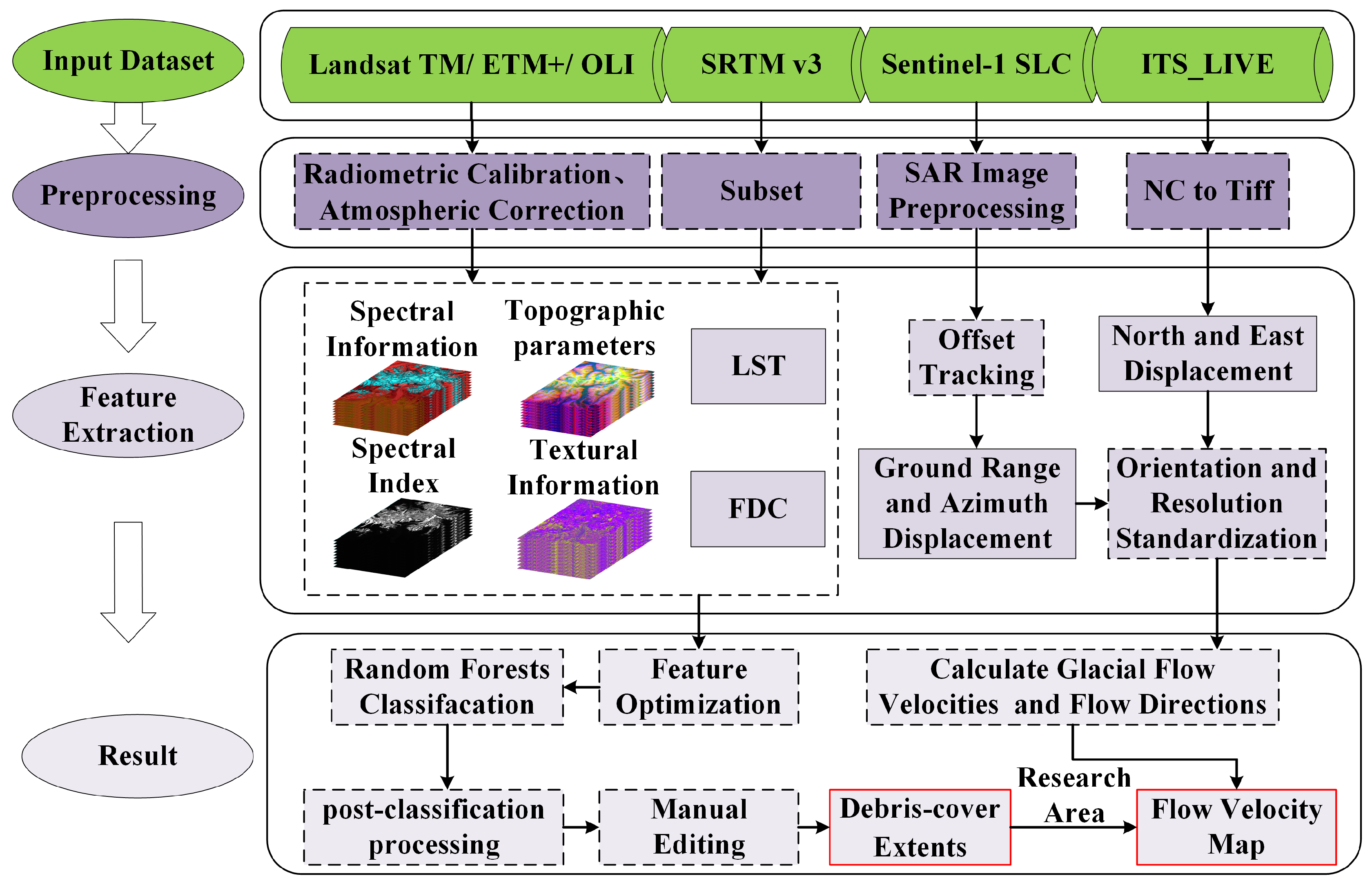
3.2. Debris Cover Extent Identification

3.2.1. Feature Extraction

Thirty feature variables were chosen for further refinement, as indicated in

Table 3. List of feature variables before optimization.

Category	No.	Feature Variable Name	Category	No.	Feature Variable Name
Spectral information	1	Blue band	Textual information	16	Entropy
	2	Green band		17	Second Moment
	3	Red band		18	Correlation
	4	NIR	Topographic parameters	19	Elevation
	5	SWIR1		20	Slope
	6	SWIR2		21	Aspect
Spectral index	7	NDVI		22	Shaded relief
	8	NDWI		23	profile convexity
	9	NDSI		24	Plan Convexity
	10	RATIO		25	Longitudinal Convexity
Textual information	11	Mean		26	Cross-sectional Convexity
	12	Variance		27	Minimum Curvature
	13	Homogeneity		28	Maximum Curvature
	14	Contrast	Others	29	LST
	15	Dissimilarity		30	FDC

. Spectral analysis utilized six Landsat imagery bands: blue, green, red, near infrared (NIR), shortwave infrared 1 (SWIR1), and shortwave infrared 2 (SWIR2). Using these bands, remote sensing indices such as the normalized difference vegetation index (NDVI), normalized difference water index (NDWI), normalized difference snow index (NDSI), and RATIO (red to shortwave infrared band ratio) were constructed. The calculation formulas for these remote sensing indices are as follows:

$$\mathrm{NDVI}=\frac{{\rho }_{NIR}-{\rho }_{red}}{{\rho }_{NIR}+{\rho }_{red}}$$

(1)

$$\mathrm{NDWI}=\frac{{\rho }_{green}-{\rho }_{NIR}}{{\rho }_{green}+{\rho }_{NIR}}$$

(2)

$$\mathrm{NDSI}=\frac{{\rho }_{green}-{\rho }_{SWIR1}}{{\rho }_{green}+{\rho }_{SWIR1}}$$

(3)

$$\mathrm{RATIO}=\frac{{\rho }_{red}}{{\rho }_{SWIR1}}$$

(4)

where ρ_NIR, ρ_red, ρ_green, and ρ_SWIR1 correspond to the reflectance values of the NIR, red, green, and SWIR1 bands, respectively.

Debris, resulting from glacier movement, feature unique textures and spatial distributions. Identifying debris cover with slope constraints and multispectral imagery yielded favorable outcomes [45]; adding texture information as a classification basis further improved the accuracy [14]. Following principal component analysis, texture information was derived via gray-level co-occurrence matrix (GLCM) operations with a 3 × 3 sliding window [46]. This texture information comprised mean, variance, homogeneity, contrast, dissimilarity, entropy, second moment, and correlation, with formulas detailed in the literature [47]. SRTM DEM provided topographical information, processed into ten features (Table 3) with ENVI 5.6 [18]. The single-period DEM did not match the image dates; however, as topographic features mainly distinguish debris from mountainous rock, this discrepancy minimally affected the classification outcomes. Changes at the glacier terminus received special attention during post-classification.

The lower temperature of debris cover compared to the surrounding terrain, due to underlying ice, facilitated debris-covered glacier boundary identification via thermal infrared remote sensing [48,49]. This study’s LST data came from the Landsat Level-2 Land Surface Temperature Science Product. Within remote sensing imagery, spectral signals of debris and bare ice frequently blend within a single pixel. To distinguish them, a linear spectral unmixing approach with debris and bare ice as endmembers generated the FDC (fractional debris cover) index as a classification feature. Debris moves along with the glacier motion, and some studies explored using glacier flow velocity for debris identification [15,50]. However, in the study area experiments, incorporating coarse-resolution flow velocity products (ITS_LIVE) as classification features did not enhance the debris identification accuracy, resulting in jagged misclassifications.

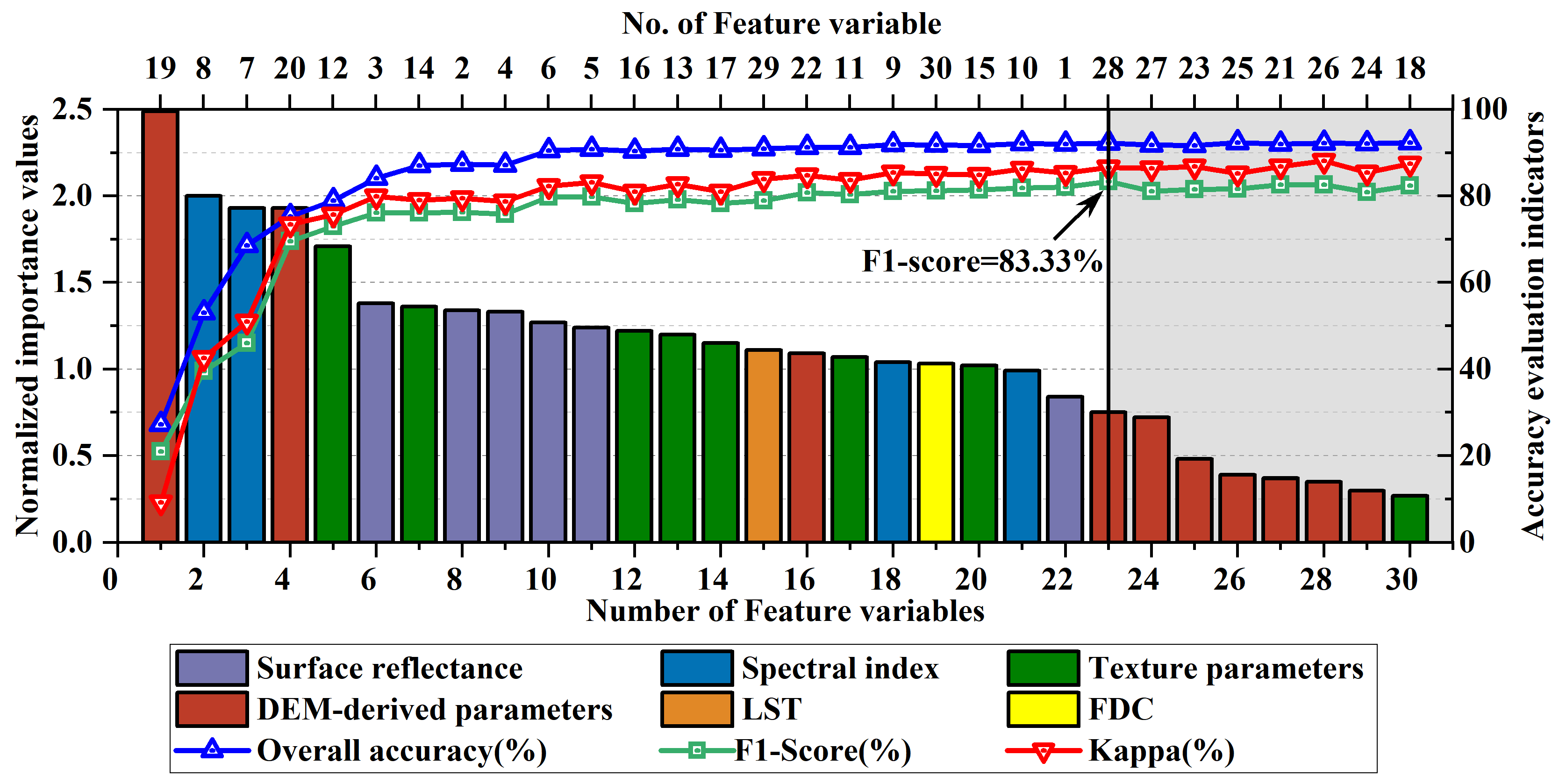
3.2.2. Feature Optimization and RF Classification

The H2020 dataset utilized the Landsat image LT51470312007236IKR00 for information gathering around Tomur Peak. This study’s sample point selection and random forest model training were based on this image. After roughly determining the proportion of various land cover types within the image frames using the H2020 dataset, we selected sample points using the stratified random sampling method. Land cover type uncertainties were verified using Google Earth^TM. Ultimately, 1726 sample points covering four debris categories—bare ice/snow, rock/bare land, and vegetation—were selected. In classifying multi-feature data with the random forest method, each feature’s importance is assessed. Within a classification and regression tree (CART), the Gini impurity is used to evaluate a feature’s classification efficacy, assigning normalized importance scores to features throughout the random forest [51].

Inherently, decision trees can select features and thresholds stepwise, but multiple local optima do not ensure a globally optimal outcome. Inspired by wrapper-based feature selection methods, this study sifted through 30 feature variables. Upon obtaining feature variable importance scores, they were ranked accordingly, and the random forest model was trained by incrementally adding features based on this ranking. The F1-score and Kappa coefficient evaluated the debris cover identification accuracy, with the F1-score as a weighted average of precision and recall [52]. The debris cover identification accuracy varied with feature count, peaking at 23 features, as depicted in Figure 3. Adhering to the highest-accuracy criterion for debris cover identification, the top 23 feature vectors were chosen as the optimal feature combination to train the random forest model. This model then classified the imagery data with the same feature combination across different periods, identifying the extent of debris cover.

Interference from moraines, seasonal snow, and shadows necessitated manual visual interpretation and correction of the automatically identified debris cover extents using remote sensing, for uses like mapping and monitoring changes in debris cover area [11,53,54,55]. Prior to manual editing, the classification results underwent median filtering to diminish “salt-and-pepper noise”, with the kernel size set to 5 × 5. For manual editing of the extent of debris cover, ArcGIS 10.8 and Google Earth^TM were employed, with visual interpretation markers including debris color texture, supraglacial ponds, glacial terminus hydrology, and topography. Debris cover identification, when combined with topographic data, effectively differentiated debris from mountainous rock, with manual editing mainly focusing on the glacier tongue terminus.

3.3. Glacier Flow Velocity Extraction

Located in a mid-latitude high mountain area, Tomur Peak Region’s severe cloud cover limited the optical image availability for the study, prompting a focus on radar remote sensing methods for extracting glacier flow velocities. While the DInSAR method provides considerable precision in velocity estimates, it requires high image coherence, due to its differential interferometric technique. Mountain glaciers’ relatively rapid flow can lead to decorrelation between images, resulting in the loss of deformation information. Conversely, offset-tracking does not encounter decorrelation issues and is minimally impacted by terrain undulations, better suiting the mountainous terrain of the study area.

Prior to cross-correlation matching, Sentinel-1A SLC images underwent processing to eliminate thermal noise, implementing multilooking and ground range projection, thereby generating backscatter intensity images. These images were subsequently registered using orbit information. For offset estimation, this study employed a frequency domain-based image cross-correlation algorithm. GCPs were uniformly placed in the master image, surrounded by 60 × 60 pixel search windows. Search windows slide across the slave image’s search area, performing cross-correlation calculations at specified step sizes. Equation (5) illustrates the frequency domain cross-correlation algorithm:

$$CC(i,j)=\mathrm{IFFT}\left(\frac{F_o(u,v)G_o^{*}(u,v)}{\left|F_o(u,v)G_o^{*}(u,v)\right|}\right)$$

(5)

In this equation, (i,j) represents the search window’s center, F₀ (u,v) and G₀ (u,v) are the fast-Fourier-transformed master and slave images, “*” indicates complex conjugation, and IFFT is the inverse Fourier transform. The correlation matrix CC measures image similarity, with its peak coordinates matching the GCP’s position in the slave image. The offset was calculated using homologous point coordinates in both master and slave images. A higher CC peak value signifies a more reliable matching result [56]. Flow velocities at GCPs exceeding 5 m/d were deemed outliers [57,58] and replaced with local weighted averages. Orbital shift errors in the total offset, arising from satellite orbit differences or attitude changes across passages, were computed and removed using a second-degree polynomial fit for global deformation. Ultimately, converting azimuthal and range displacement into north and east directions, based on radar incidence angle and satellite orientation, and performing vector composition yielded the glacier’s planar flow velocity.

4. Result

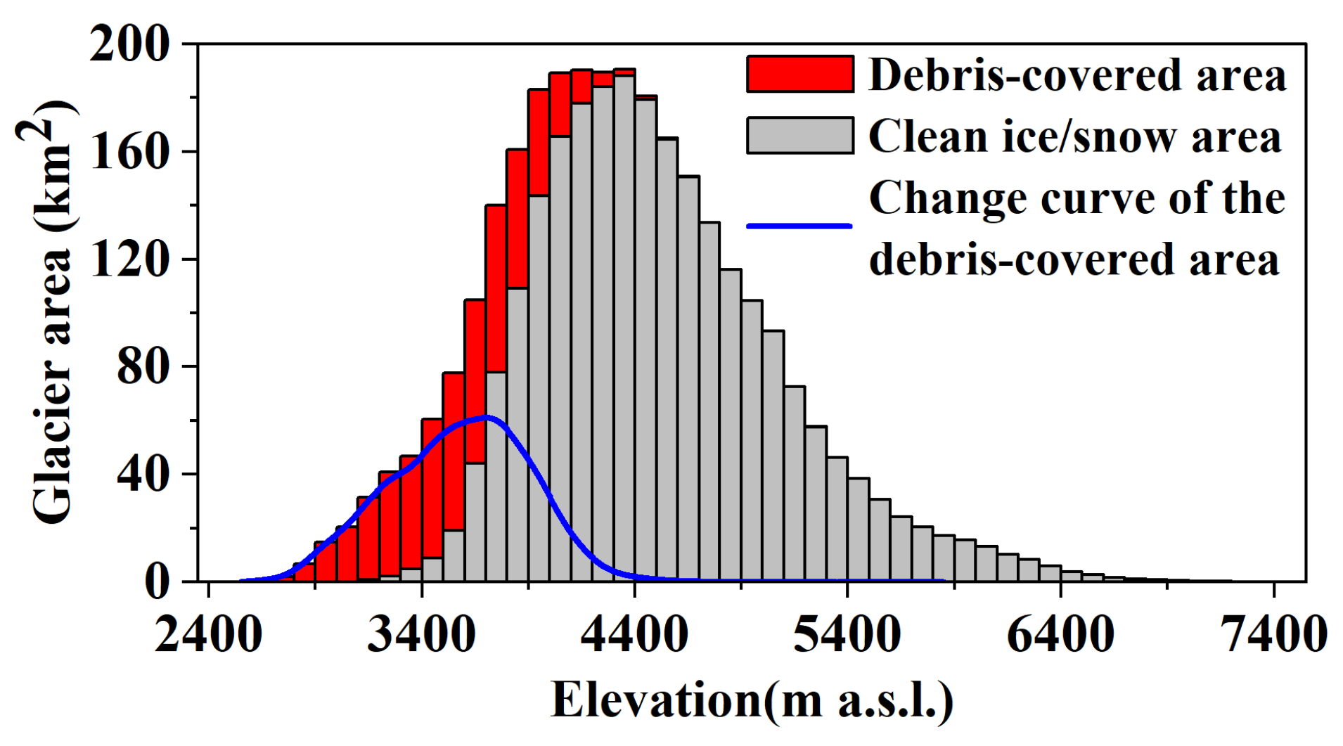
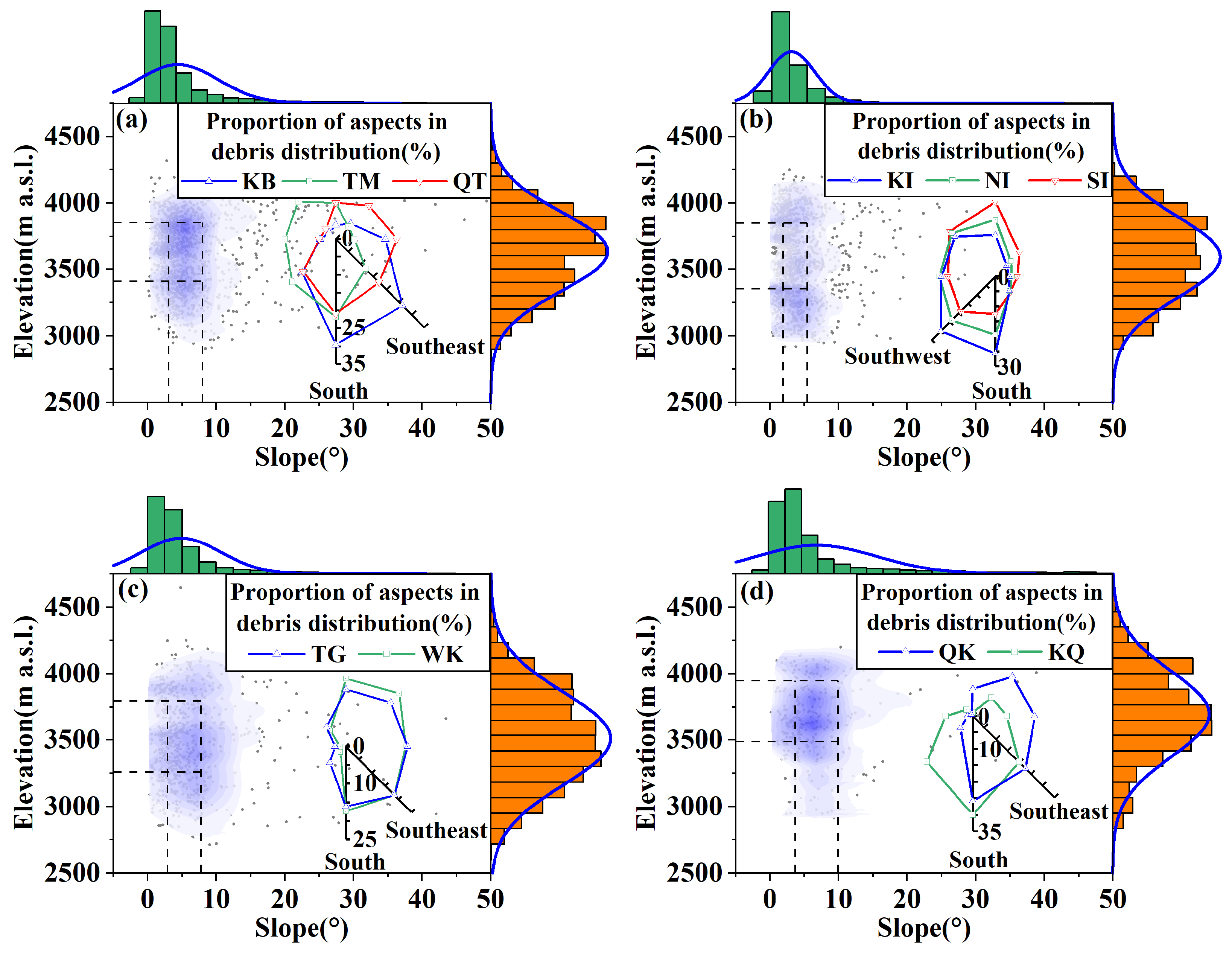
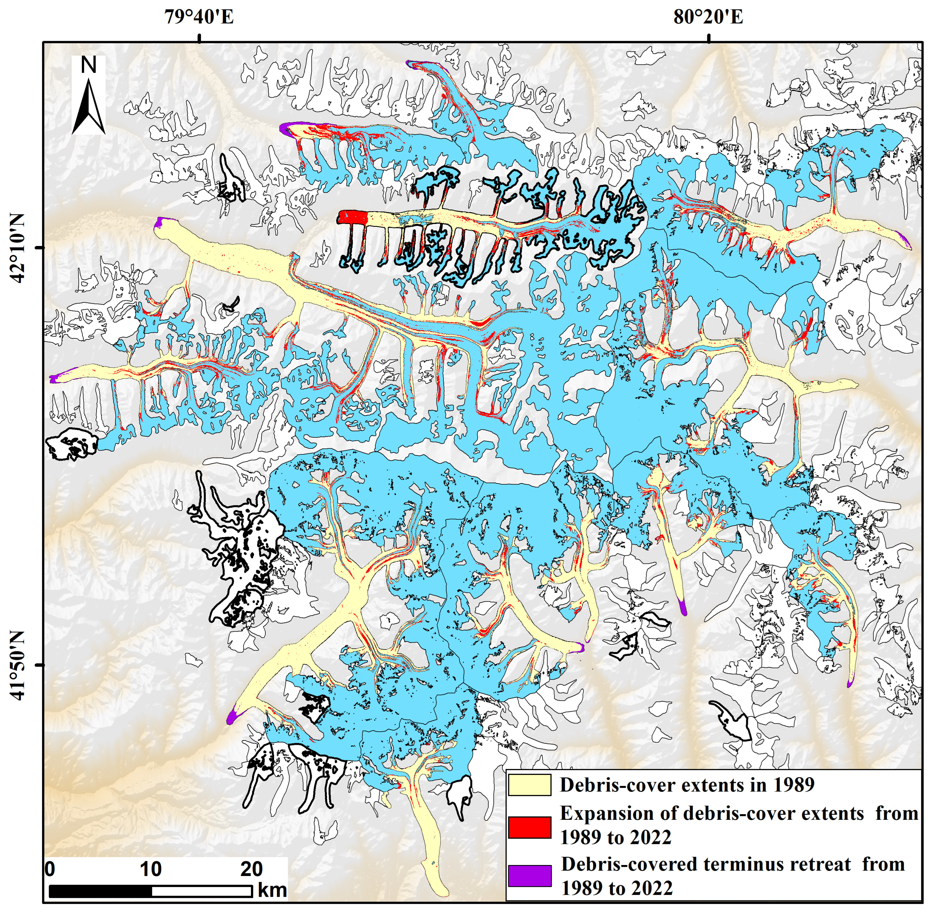
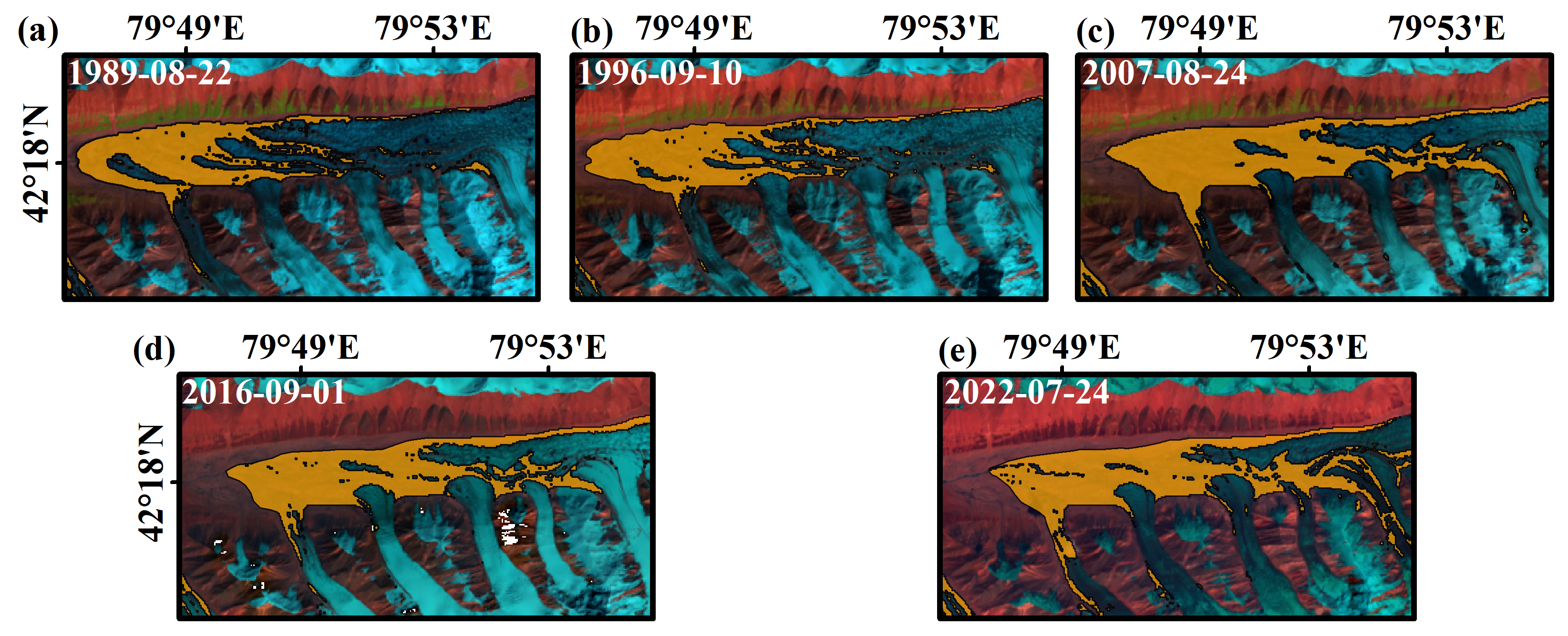
4.1. Spatial Distribution of Debris Cover

The identification results of the extent of debris cover in 2022 were analyzed, showing that the area of debris cover within the study region (409.2 km²) accounted for 22.8% of the total glacier area. The area–elevation distribution of the debris cover, as illustrated in Figure 4, shows that the debris was distributed across an elevation range of 2500 m to 4700 m. A total of 75% of the debris area was concentrated between 3300 m and 3900 m, while glaciers from 2500 m to 3100 m elevation were entirely debris-covered.

Spatial distribution patterns of debris cover across different regions are detailed in Figure 5. The elevation’s normal distribution for debris cover predominantly fell within the interquartile range of 3250 m to 3950 m, with its slope distribution similarly within 3° to 10°. Given debris primarily forms on glaciers’ gentler downstream slopes, its elevation and slope distributions are notably focused, starkly contrasting with clean ice surfaces. This rationale underscores the importance of elevation and slope as key features in the debris classification process, as depicted in Figure 3. In diverse regions, slight variances in the debris distribution’s elevation and slope predominantly stem from the glaciers’ inherent topographic features. Glaciers of greater length and scale show a narrower range in their debris slope distribution. On Tomur Peak’s northwest, larger glaciers such as North Inylchek, South Inylchek, and Kaindy exhibited a concentrated slope distribution of 1.9° to 5.4° (Figure 5b), markedly gentler and more focused than those in other regions. The aspect of the debris distribution mirrored the glaciers’ orientation.

4.2. Changes in the Extent of Debris Cover

Table 4. Changes in the extent of debris cover on glaciers in the study region from 1989 to 2022. The abbreviations of glacier names are detailed in Figure 1. ∆DebrisCov, debris coverage change; Abs. rate, absolute rate; Ann. rate, mean annual rate; Cum. area, cumulative area.

Glacier or Region	∆DebrisCov (1989–1996)		∆DebrisCov (1996–2007)		∆DebrisCov (2007–2016)		∆DebrisCov (2016–2022)		∆DebrisCov (1989–2022)
	Abs. Rate	Ann. Rate	Abs. Rate	Ann. Rate	Abs. Rate	Ann. Rate	Abs. Rate	Ann. Rate	Cum. Area	Cum. Rate
	km2·a−1	%·a−1	km2·a−1	%·a−1	km2·a−1	%·a−1	km2·a−1	%·a−1	km2	%
KB	−0.10	−0.43	0.05	0.24	0.01	0.05	0.05	0.24	0.24	1.06
TM	−0.46	−0.72	0.30	0.48	−0.09	−0.13	1.11	1.75	5.22	8.04
QT	−0.29	−0.72	0.19	0.49	0.02	0.04	0.45	1.11	2.51	6.14
KI	−0.09	−0.52	0.01	0.07	0.17	1.02	0.62	3.45	4.91	28.99
NI	−0.41	−1.69	0.51	2.40	0.57	2.17	0.58	1.83	10.89	44.70
SI	−0.87	−1.12	0.71	1.00	0.56	0.73	1.79	2.15	16.69	21.60
TG	−0.39	−1.00	0.24	0.67	0.53	1.39	0.67	1.55	8.78	22.74
WK	−0.37	−1.50	0.35	1.56	0.44	1.73	0.42	1.42	7.40	29.84
QK	−0.37	−2.73	0.26	2.32	0.03	0.23	0.30	2.17	1.79	13.05
KQ	−0.47	−2.72	0.31	2.23	−0.06	−0.33	0.57	3.52	2.39	13.77
SY	0.00	0.20	0.11	9.80	0.02	0.75	0.31	13.95	3.02	276.79
MS	0.04	0.92	0.23	4.40	0.07	0.99	0.42	5.36	5.59	115.71
Total	−3.78	−1.09	3.27	1.02	2.26	0.65	7.31	1.96	69.41	20.00

and Figure 6 show the changes in the extent of debris cover on glaciers within the Tomur Peak Region from 1989 to 2022. Over 34 years, Tomur-type glaciers saw a 69.4 km² expansion in debris cover, marking a 20.0% increase. The significant expansion of debris-covered areas on glaciers may have influenced the overall melting state in the Tomur Peak Region. From 1989 to 1996, an unusual reduction in debris cover area was observed across glaciers, with a rate of −1.09%·a⁻¹. Imagery observations indicated the extension of bare ice areas downward with glacier motion. In other time frames, all glaciers’ debris cover expanded, with the highest annual growth rate of 1.96% between 2016 and 2022, and a subsequent rate of 1.02% from 1996 to 2007.

Upward evolution, delineated by the spread of debris cover at the interface between debris-covered and clean ice areas, represented the predominant form of debris expansion in the study area. Debris expansion at glacier termini, triggered by glacier advance and surging, was more common for smaller glaciers. Larger glaciers typically possess more stable internal structures. During the study period, only the North Inylchek Glacier exhibited surge phenomena [59], resulting in the expansion of its terminal debris. Tomur Glacier, Koxqar Glacier, and Qiongtailan Glacier, located on the southwestern side of the Tomur-Khan Tengri range, showed relatively little expansion in supraglacial debris cover. Conversely, glaciers at Tomur Peak’s northern base saw a significantly higher debris area growth rate than those on the southern slope. These differences in the change in debris cover area between the northern and southern slopes can be attributed to (1) the northern slope’s glaciers having numerous narrow tributaries and pronounced fracture faces, aiding in the debris’ upward evolution; (2) the relatively isolated and smaller accumulation areas on the northern slope, which might have experience intensified mass loss due to climate warming, leading to the rapid exposure and subsequent formation of debris from moraine material at the glacier tongue; and (3) variances in sunlight exposure and climate change impacts between the slopes potentially influencing debris expansion rates.

4.3. Glacier Flow Velocity Extraction Results

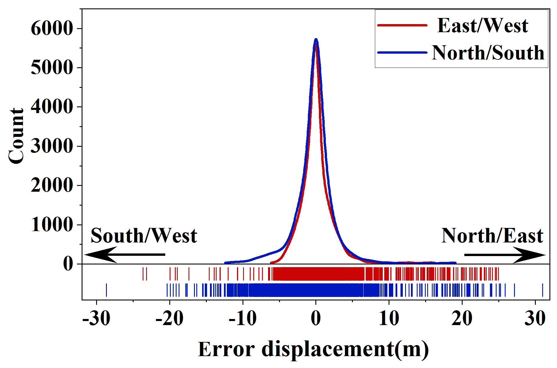
4.3.1. Error Analysis

Deformation in non-glacial areas (such as bare land) is theoretically static, serving as reliable control points for validating velocity extraction accuracy [60]. Numerous control points, well-distanced from the glaciers, were selected in the flow velocity extraction images, with their displacement values illustrated in Figure 7. Displacement values in static areas, both east–west and north–south, exhibited a roughly normal distribution, indicative of the random error distribution within the velocity extraction outcomes. The east–west directional mean error stood at 1.79 m with a standard deviation of 2.69 m, whereas the north–south errors slightly exceeded the east–west, with a mean error of 2.39 m and a standard deviation of 4.40 m.

Errors in extracting glacier velocities chiefly arise from image registration inaccuracies, errors induced by terrain, and geocoding discrepancies [61]. The primary errors occur during the image cross-correlation phase; image resolution and algorithmic limitations restrict the accuracy of velocity results. Additionally, complex surface changes on glaciers, such as precipitation, snowfall, and melting, may lead to inaccurate image matching. This study opted for shorter temporal baselines and focused on stable debris-covered areas to reduce the introduction of errors from external factors, with interpolation addressing “void values” or abrupt velocity changes due to misregistration. Given the expansive riverbeds of Tomur-type glaciers and the gentle debris-covered terrain, the terrain’s impact on the flow velocity extraction was minimal. The SRTM v3’s average absolute error in glacier regions is approximately ±8 m [62], ensuring its reliability for geocoding flow velocity extractions.

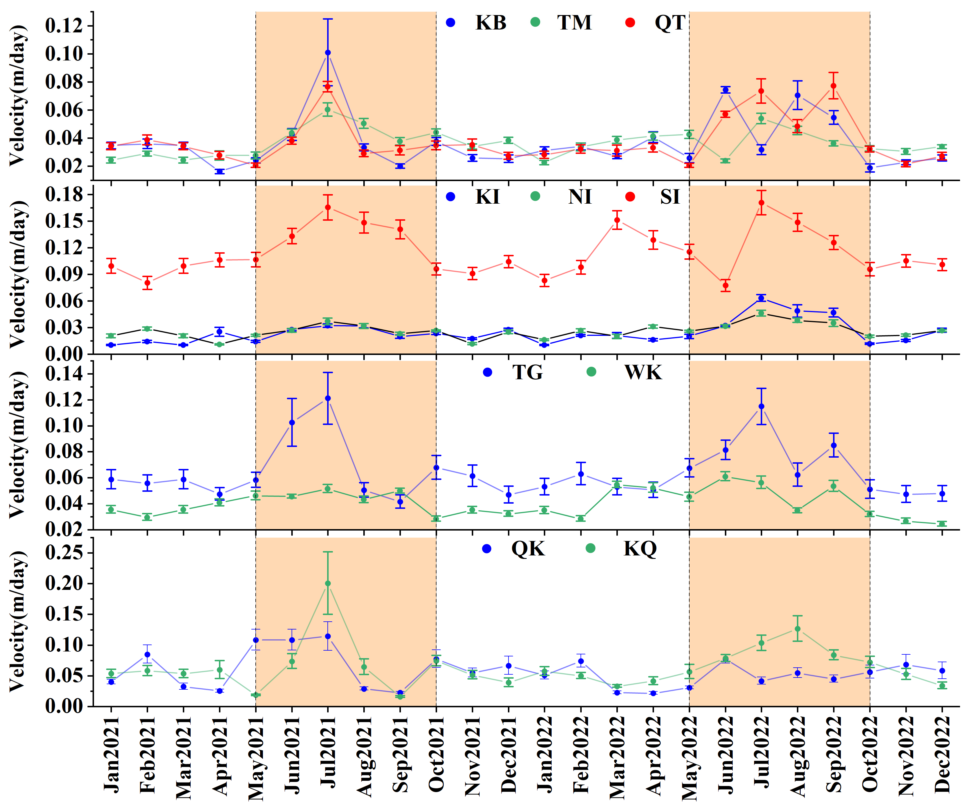
4.3.2. Seasonal Velocity Variation

Flow velocity variations along the central flow lines of glaciers are spatially and temporally stable, offering a representative overview of overall glacier flow changes. The SAR offset-tracking method was employed to extract monthly flow velocities of Tomur-type glaciers for the years 2021 and 2022. Figure 8 illustrates the variation in mean flow velocity along the glaciers’ central flow lines.

Glacier flow velocity fluctuates throughout the year, with stronger fluctuations during the melt season compared to the non-melt season. Moreover, mean velocities are generally higher in the melt season than in the non-melt season, with peak velocities frequently occurring during this period, particularly in July. Increased glacial meltwater and precipitation enhance drainage at the glacier’s base during the melt season, promoting basal motion and thereby accelerating glacier flow [42,63,64]. Furthermore, rising ice temperatures can intensify the plastic deformation of glaciers, and short-term material replenishment may heighten gravitational stress, albeit these elements have a secondary influence on glacier flow velocity.

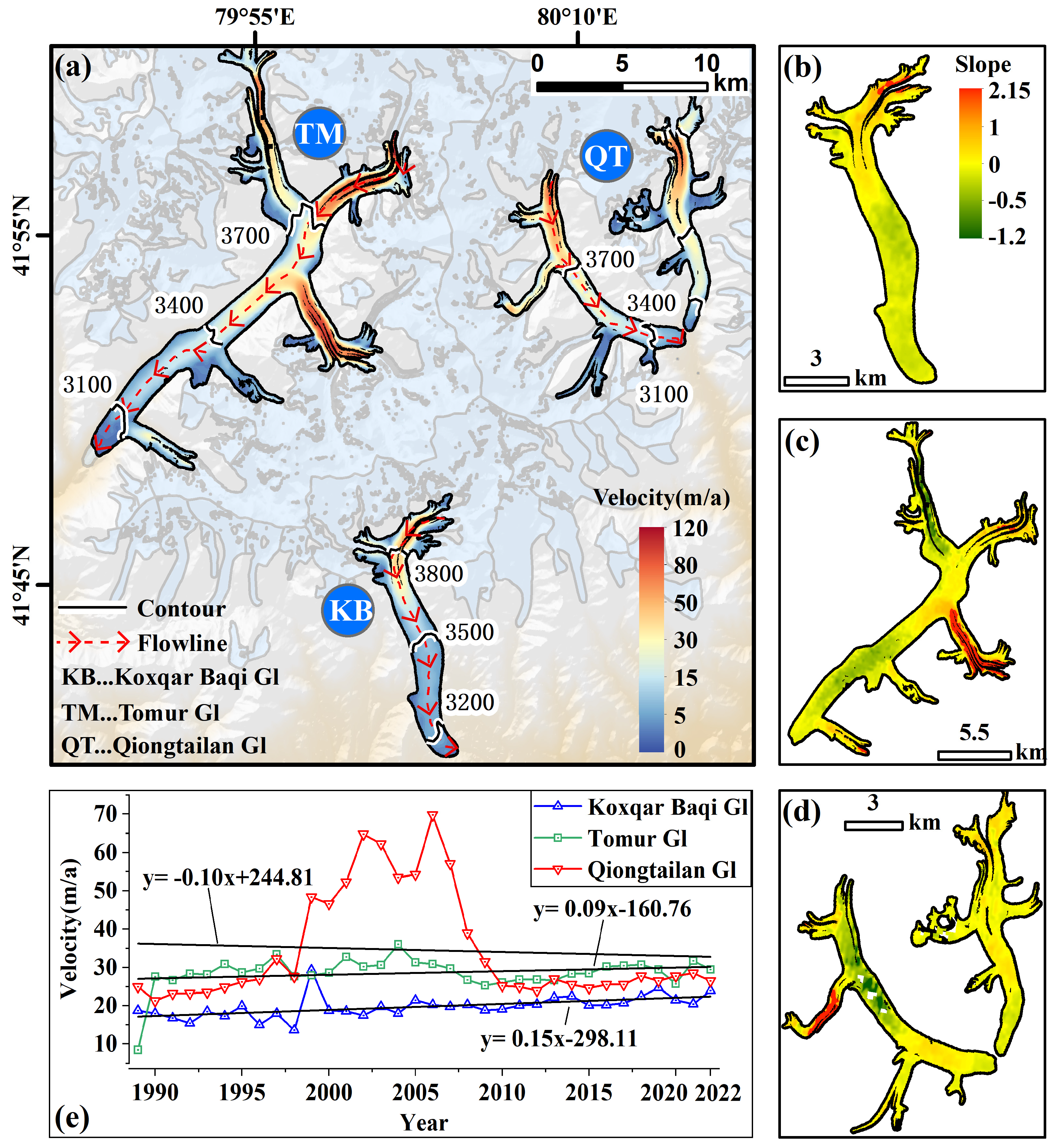
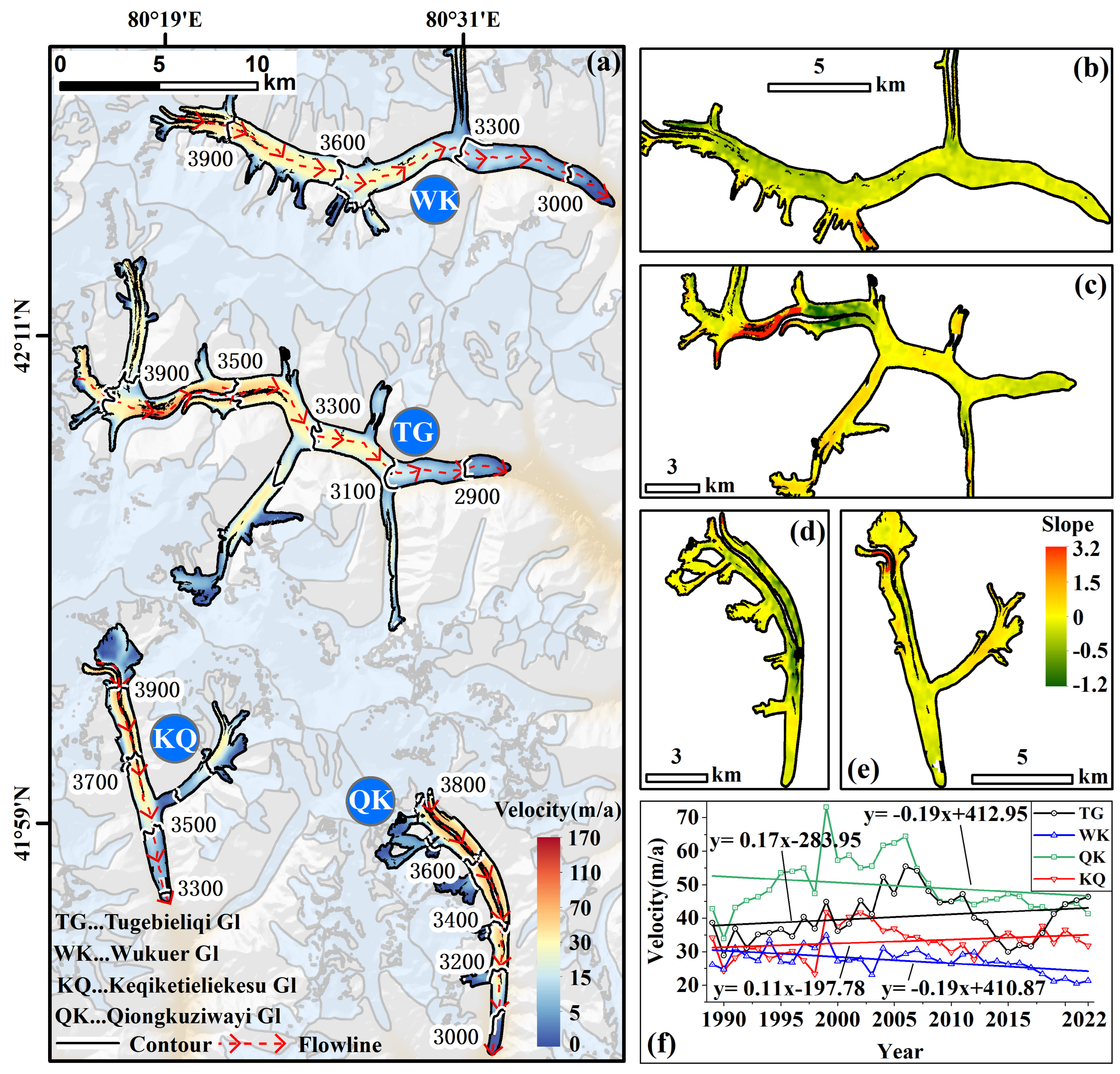
4.4. Spatiotemporal Velocity Variations

We integrated the ITS_LIVE dataset, the S1 dataset, and the glacier velocity extraction results from this study to construct a time series from 1989 to 2022. The three datasets were generated using consistent principles, namely image feature tracking. The analyzed values were averaged to prevent any single value from having an excessive error. Consequently, the time series constructed from these values reliably reflected the trends in glacier velocity.

4.4.1. Northwest Region

A time series analysis showcasing flow velocities for three glaciers in the northwest region of the Tomur-Khan Tengri Mountain Range is presented in Figure 9, with the changes in mean velocity along the central flow lines over 34 years depicted in Figure 9e.

As demonstrated in Figure 9a, the flow velocities exhibited a downward trend from the glaciers’ upper reaches to their lower extents, with velocities along the central flow lines surpassing those at the glacier edges. Owing to its large size, the average peak velocity of the South Inylchek Glacier reached 149.7 m/a. Nearly three-quarters of the main glacier stream (from 3400 m a.s.l to 4200 m a.s.l) exhibited exceptionally high movement speeds. In the last 50 years, Central Tianshan’s glaciers have experienced notable mass reductions and ongoing thinning [65,66], culminating in a widespread slowdown of glacier movement speeds. Kaindy Glacier was an exception, showing a notable uptick in flow velocity between 3450 m and 3680 m. Li et al. [66]’s research indicated that while the glacier’s forefront underwent substantial thinning between 2000 and 2012, the segment from 3500 m to 3700 m slightly thickened. A marked discrepancy in glacier thickness alterations on either side of the 3500 m contour line induced an elevation in local slope, concurrently amplifying the gravitational driving stress and thereby accelerating the glacier flow velocities.

4.4.2. Southwest Region

Time-series analyses of glacier flow velocities in the southwest sector of the Tomur-Khan Tengri Mountain Range are illustrated in Figure 10.

The large size of the tributaries of the Tomur Glacier significantly impacted the gradient distribution of the glacier velocity (Figure 10a). In the ablation zones of the Tomur and Koxqar Glaciers, certain areas were covered by thick debris layers exceeding 2 m in depth, which significantly slowed down the thinning of these glaciers. Despite a reduction in flow velocities downstream (Figure 10b,c), these glaciers’ overall velocity trend was upward (Figure 10e). The West Qiongtailan Glacier saw an unusual increase in flow velocity between 1999 and 2009 (Figure 10e), with the mean velocity at the flow line reaching 69.7 m/a in 2006, nearly 2.8 times that of the pre-1999 period. This was accompanied by a notable thickening in the glacier’s accumulation area (3430 m to 3700 m) [66]. The acceleration in the West Qiongtailan Glacier’s western branch from 1999 to 2009 might have been primarily due to thermodynamic changes at the glacier base. An increase in ice temperature likely facilitated the deformation of basal sediments and elevated the pore water pressure, thereby intensifying basal sliding or potentially causing detachment [67].

4.4.3. East Region

Time-series analyses of glacier flow velocities in the eastern sector of the Tomur-Khan Tengri Mountain Range, as depicted in Figure 11.

Among the four glaciers, the Qiongkuziwayi Glacier maintained the highest overall flow velocity. Influenced by the confluence of four western tributaries, average velocities at elevations above 3200 m exceeded 30 m/a (Figure 11a). In comparison with the Tugebieliqi and Wukuer glaciers, despite the Tugebieliqi Glacier extending only 3.7 km more, its ice volume amounted to 2.2 times that of Wukuer’s, guaranteeing higher flow velocities due to the ample material supply. Over a 34-year period, the overall velocities of Wukuer and Qiongkuziwayi Glaciers exhibited a decreasing trend (Figure 11b,d,f), while those of Tugebieliqi and Keqiketieliekesu Glaciers demonstrated an increasing trend (Figure 11c,e,f). Synthesizing data from Figure 9, Figure 10 and Figure 11, it is evident that increases in glacier flow velocity generally occurred at tributaries and their confluence points, including the southern tributaries of the Tomur Glacier and the segment between 3580 m and 3830 m of the Tugebieliqi Glacier. Areas of velocity increase are typically situated near the glacier accumulation zones, where elevations are high, melt rates are low, and material supply is abundant, resulting in increased gravitational stress between these areas and the continually thinning main glacier tongues, leading to an increase in flow velocities.

5. Discussion

5.1. Accuracy Assessment of Debris Cover Identification

Employing the optimal feature combination, the random forest classifier attained an overall classification accuracy of 92.23%, a debris cover identification accuracy of 83.33%, and a Kappa coefficient of 0.87 (Figure 3), falling within an acceptable range, with a Kappa coefficient greater than 0.8 deemed an acceptable accuracy range [68,69]. To examine the differences in performance of various machine learning methods in debris cover identification and the impact of study area size on this accuracy, the glaciers in the Tomur Peak Region and the Koxqar Glacier were classified with various machine learning methods, with their accuracies subsequently validated, as illustrated in

Table 5. Accuracy assessment of various machine learning methods for debris-cover identification in the Tumur Peak Region and Koxqar Baqi Glacier.

Feature Composite	Classifier	Tomur Peak Region		Koxqar Baqi Gl
		F1-Score	Kappa	F1-Score	Kappa
Spectral information	Random Forest	56.0%	0.53	67.8%	0.65
	Maximum Likelihood	42.3%	0.32	45.8%	0.35
	Support Vector Machine	27.9%	0.22	29.5%	0.25
	Artificial Neural Network	53.3%	0.49	61.4%	0.48
All features	Random Forest	82.4%	0.76	85.4%	0.84
	Support Vector Machine	73.2%	0.65	76.0%	0.69
Selected features	Random Forest	83.3%	0.87	88.6%	0.86

.

The accuracy of classification methods relying solely on spectral information for debris cover identification was insufficient, failing to meet the accuracy requirements for remote sensing classification. The random forest method, when considering all feature vectors, demonstrated high accuracy in debris cover identification, a metric that could be further enhanced through feature optimization. Overall, the feature optimized random forest method demonstrated significant advantages in debris cover identification. Remote sensing spectral information of mountain glaciers exhibits high spatial variability, with the characteristics of debris cover, including the distribution slope and surface temperature range, also showing considerable variation. The more limited the research scope, the more concentrated the distribution interval of debris cover features, leading to an enhanced debris identification effect. Irrespective of the classification method employed, the accuracy of debris cover identification within the Koxqar Glacier range surpassed that of the experiments conducted across the entire Tomur Peak Region, underscoring the influence of study area size on the accuracy of debris cover identification.

Although visual interpretation markers in debris-covered areas of Tomur-type glaciers are abundant and explicit, the manual editing process may still introduce subjectivity. Given the complex surface conditions in high mountain areas, the accuracy of digital elevation models (DEM) and surface temperature products may be compromised [64,70], introducing errors for which there are currently no effective solutions. Another source of uncertainty is that temporal mismatches in topographical data may result in the misclassification of features at glacier termini, necessitating adjustments during the manual editing process.

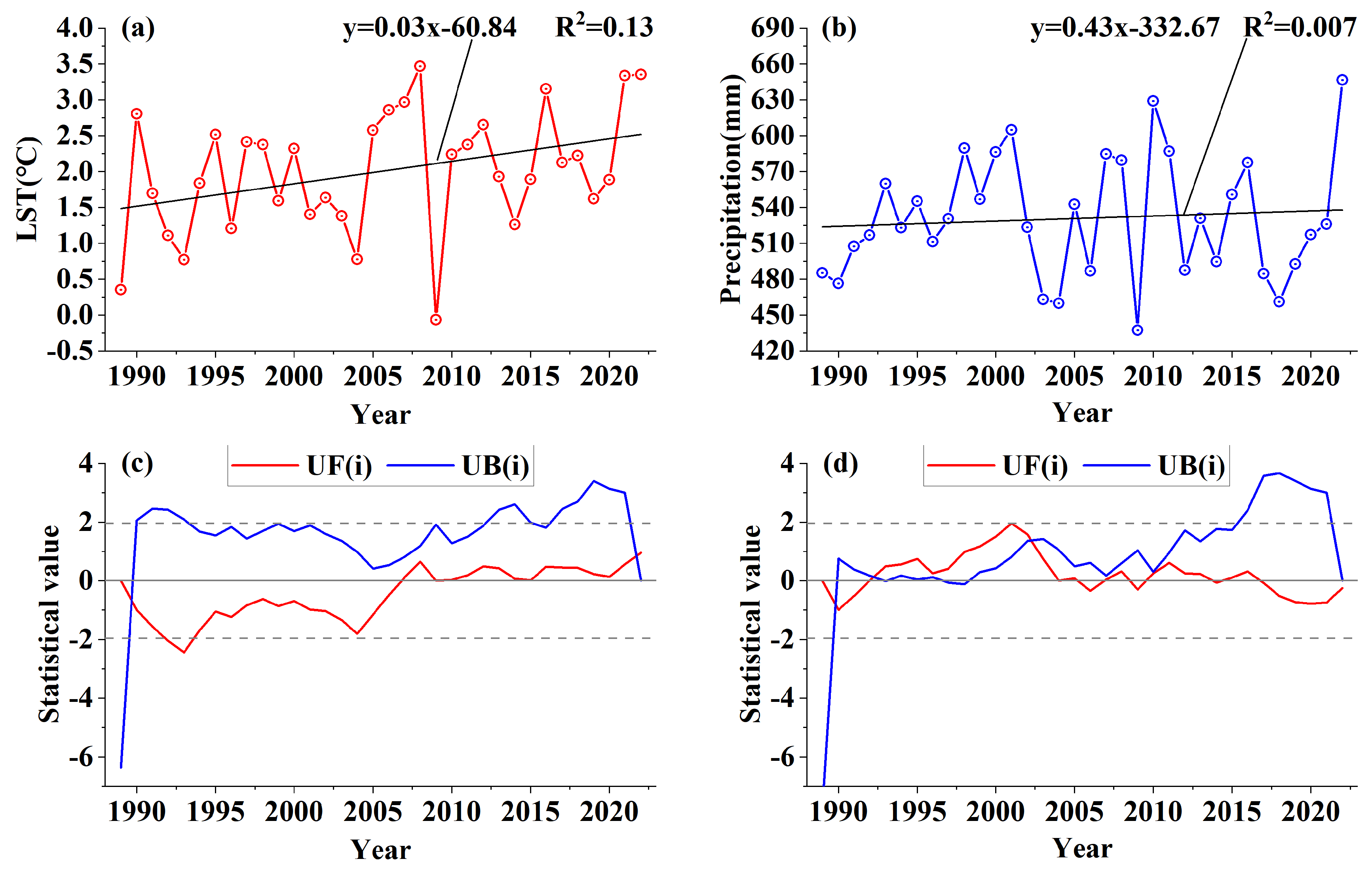
5.2. Determinants of Debris Cover Upward Evolution

Temperature and precipitation respectively govern the melting and accumulation processes of glaciers, thereby influencing their development and morphological evolution. This study obtained surface temperature and cumulative precipitation data for the melt season in the Tomur Peak region from 1989 to 2022, sourced from the ERA5 dataset, and conducted trend analyses, as depicted in Figure 12. The results of the linear regression analyses revealed a gradual upward trend in both surface temperature and cumulative precipitation within the study area over the preceding 34 years (Figure 12a,b).

Glacier length and area may expand due to glacier advancement or surging, consequently leading to the expansion of the extent of debris cover. Glacier advancement and surging are driven by complex factors, among which changes in temperature and precipitation play a significant role in affecting a glaciers’ internal stability and material accumulation upstream, often triggering surging. Upon examining the spatial distribution of surging glaciers in the Tianshan region, it was noted that these glaciers are predominantly situated in the central and western parts of the Tianshan mountains, regions where the temperature incrementally increases and precipitation gradually rises annually, with a notable concentration of surging glaciers in the Tomur Peak area [59]. The advancing and surging glaciers around Tomur Peak are predominantly small in size and not universally debris-covered; thus, the debris cover expansion attributed to glacier advancement and surging represents only a minor portion. The predominant mechanism behind debris cover expansion is its upward progression, specifically, the expansion of debris at the interface between debris-laden and clean glacier ice. In the context of global warming, similar trends in debris upward have been documented in debris-covered glaciers in diverse locations, such as the Zmutt Glacier in the Alps [71] and glaciers in the Greater Caucasus region [12]. In regions maintaining a stable glacier mass balance, the area covered by debris has not exhibited a significant increase [72].

Debris cover formation predominantly occurs through two processes: the exposure of englacial debris by glacier movement and melting, and the accumulation of weathered rock and fallen debris on the glacier surface, forming supraglacial debris. A minor increase in precipitation impacts glaciers significantly less than the effects of temperature elevation. Glaciers in the Tomur area are undergoing continuous mass loss. As englacial debris is exposed through melting, the area covered by debris continues its upward evolution. Considering the Mushketova Glacier as an example, which has exhibited significant debris cover expansion, despite a modest retreat at the glacier terminus, the debris cover area on this glacier has still expanded by nearly 1.2 times over 34 years (Table 4, Figure 13).

The Mann–Kendall test results for precipitation and temperature changes in the study area indicated a downward temperature trend and an upward precipitation trend between 1989 and 2006 (Figure 12c,d), contributing to a slower glacier mass loss. Certain studies verified a reduction in the glacier mass loss rate in the Tomur area during this period [73]. In addition to climatic factors, elements like debris cover effects, low ice temperatures, and high altitudes contribute to the glaciers in the Tomur area being more stable than those in other central Tianshan Mountain regions [40]. This may related to the minor decrease in the debris cover area in the study area from 1989 to 1996. Considering the source of debris material, glacier movement erodes the underlying and surrounding rocks, while accumulated moraine material is redistributed with glacier movement, continually supplying materials for debris cover formation. A warming climate and thinning glaciers may lead to permafrost melting and high-altitude mountain slope instability [74], triggering increased rockfalls, ice–rock avalanches, and snow–rock avalanches, which transport significant debris to glaciers [75,76], thereby facilitating the upward evolution of debris cover.

5.3. Control Factors of Glacier Flow Velocity

Gravity triggers internal deformation and basal sliding within glaciers, with the intensity of gravitational driving stress being dictated by the glacier’s thickness and slope. Therefore, glacier flow velocity predominantly relies on the glacier’s thickness and slope [3,20]. Additionally, a glacier’s size, shape, length, and topographical attributes (including elevation, altitude, and aspect) also exert an influence on its flow velocity, though to a lesser extent. Typically, the glacier’s upper and middle sections are thicker than its lower parts, with a steeper slope, resulting in a general trend of decreasing glacier flow velocities from upper to lower reaches. This pattern of velocity distribution has been documented in numerous glaciers throughout the high-mountain regions of Asia [43,77,78,79].

In the context of global climate warming, glaciers generally exhibit a thinning trend, resulting in decreased velocities for most glaciers in the high-mountain areas of Asia. Notably, glaciers in the Nyainqentanglha region have experienced the most significant deceleration, with a decrease of (37.2 ± 1.1)% per decade [20,80]. Conversely, glaciers located in the western part of the Kunlun Mountains and the Karakoram region, where the glacier mass is nearly balanced or slightly increasing, have seen a slight acceleration in flow velocities [81,82]. The annual mean velocity for all glaciers in the study area was analyzed statistically, revealing a gradual deceleration of overall glacier velocities in the Tomur region at a rate of −4.0% per decade. However, when examining individual glaciers, significant variability in flow velocities emerged, marked by considerable seasonal differences. Specifically, certain glaciers registered an increase in flow speeds over the 34-year period, a phenomenon not solely explainable by changes in glacier thickness. Basal sliding constitutes the greatest uncertainty in determining glacier flow velocities. Numerous studies agreed that variations in temperature and precipitation in the study area control the discharge at the glacier bed. Changes in subglacial water pressure influence the intensity of basal sliding, thereby causing fluctuations in glacier flow velocity [83,84]. During the mid-study period, the Kaindy and Qiongtailan Glaciers displayed marked increases in flow velocity, notwithstanding stable glacier terminus lengths, indicative of rapid material transfer and accumulation—a phenomenon characteristic of swift glacier advance [66]. More specifically, ongoing accumulation in the upper zones and alterations in thermal conditions at the glacier’s base may facilitate enhanced basal sliding or even detachment, resulting in glacier material moving from the accumulation zones to the ablation areas, thus culminating in periods of rapid movement [67].

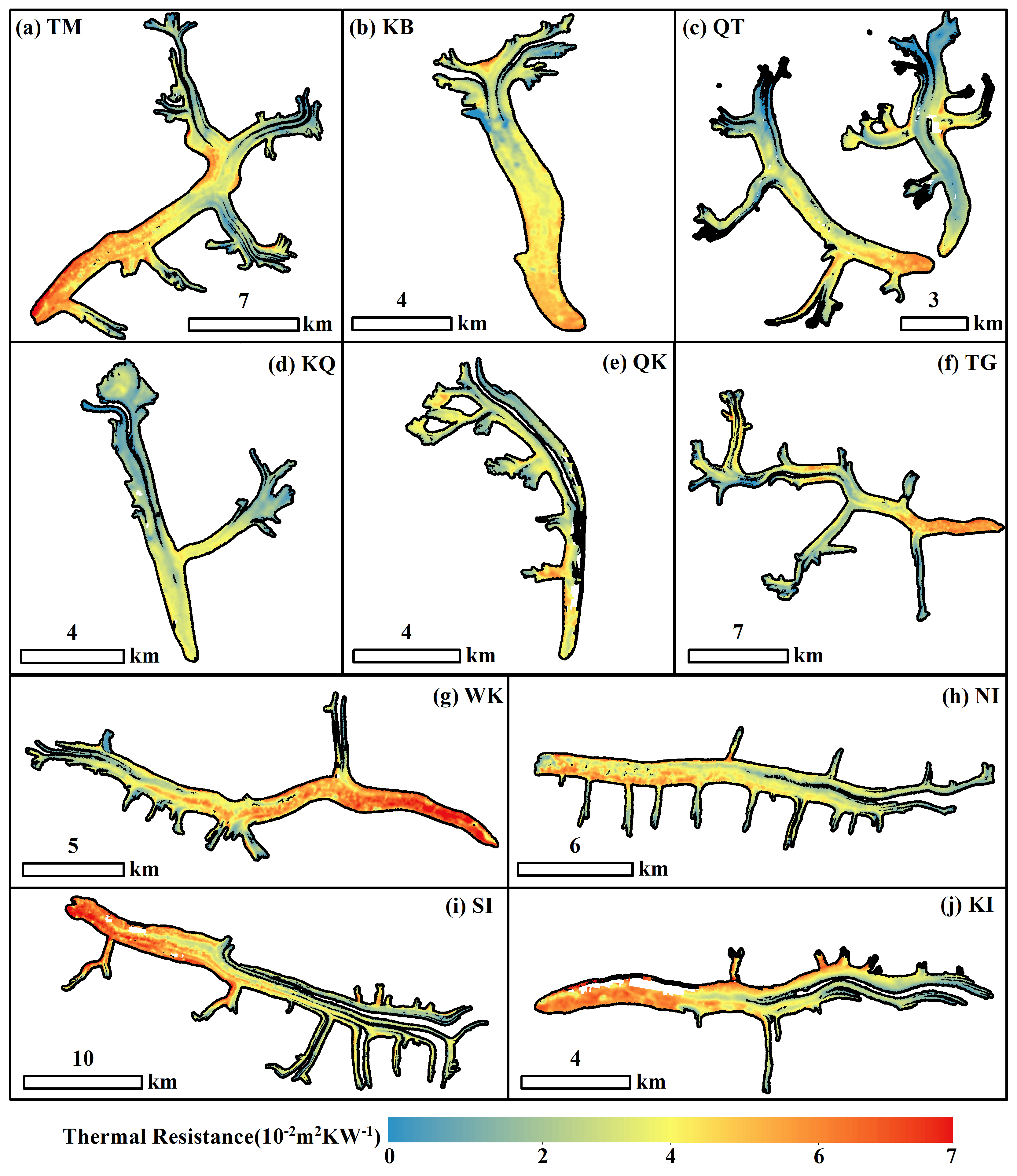
5.4. Relationship between Glacier Movement and Debris Distribution

The interaction and feedback mechanisms among climate, supraglacial debris, hydrological conditions, and glacier dynamics collectively control the ablation and morphological evolution of debris-covered glaciers, as illustrated in Figure 14. Identifying the extent of debris cover is a fundamental task in the study of debris-covered glaciers. Glacier dynamic processes are the primary driving forces behind the formation, transfer, and accumulation of supraglacial debris. The glacier’s horizontal velocity field governs the transportation of debris on the ice surface and the variations in local debris thickness.

The method of estimating the distribution of debris thickness on glaciers in the Tomur Peak region was based on remote sensing-derived land surface temperature combined with the energy balance equation, using the debris thermal resistance as a proxy indicator for debris thickness. The results are shown in Figure 15. Similar methods have been applied to study typical debris-covered glaciers in the Himalayas [85,86], Gongga Mountain [87], the Caucasus Mountains, and the China-Pakistan Economic Corridor [88]. These studies demonstrated a common characteristic: the debris thickness at the glacier terminus was greater than that in the upper middle part of the ablation zone, with the thickness increasing closer to the terminus. This characteristic is in agreement with observations and simulations of the glacier debris thickness distribution in many regions of Asian high mountains and can be regarded as a widespread phenomenon [89,90,91].

As seen in the cross-sectional profile of the glaciers, the debris thickness on both sides of the glacier generally exceeded that observed along the central flow line. A special case occurs when one side of the glacier receives a substantial input from tributaries, resulting in greater debris thickness on that side compared to the central flow line and the opposite side, as observed on the south side of the North Inylchek Glacier tongue (Figure 15h) and the north side of the Kaindy Glacier tongue (Figure 15j).

During the formation of supraglacial debris, glacier movement acts like a “conveyor belt”: debris are continuously transported to the glacier terminus, and existing debris typically remain on the glacier surface. As the glacier velocity gradually decreases to zero, the position of the debris stabilizes, and the continuous accumulation of debris leads to an increase in debris thickness. This process results in debris being primarily distributed in the middle to lower parts of the glacier, with the thickness increasing closer to the glacier terminus.

Due to the lack of extensive measured parameters (e.g., debris porosity, debris density, and glacier ablation rates), we adopted the analytical model proposed by Anderson et al. [22] instead of a numerical model to analyze the formation of the debris thickness distribution pattern. This approach simplifies the complex physical processes inherent in glaciers, only considering the instantaneous state of the glacier system. In the ablation zone of a glacier, the debris thickness can be expressed as

$$d(x)=\frac{1}{U_s}{\displaystyle {\int }_{x_e}^x\frac{Cb}{(1-\varphi )\rho }}dx$$

(6)

C represents the concentration of moraine within the ice, b represents the glacier ablation rate under the debris cover, φ represents the porosity of the debris, ρ represents the density of the debris, U_s represents the glacier surface velocity, d represents the debris thickness, x represents the distance from the glacier’s origin, and x_e denotes the position where debris first appears. Assuming C, φ, and ρ are constants throughout the glacier, the debris thickness d is controlled by the glacier surface ablation rate b and the glacier surface velocity U_s. Using the Koxqar Glacier as a case study to analyze the trend of debris thickness variation, the relationship between debris thickness and glacier elevation is shown in Figure 16.

In the elevation range of 3500 m to 3880 m, the debris thickness variation is mainly controlled by the ablation rate. Assuming a constant glacier surface velocity U_s, as the debris thickness increases, the glacier ablation rate b will continuously decrease, leading to a reduction in the debris emergence rate and a slower increase in debris thickness. This explains the trend observed in the 3500 m to 3880 m elevation range. As the debris thickness continues to increase, the glacier ablation rate b approaches zero, and the debris emergence rate also approaches zero. At this point, the glacier ablation rate b and the concentration of debris C no longer influence the debris thickness growth rate. Below 3500 m, the glacier flow velocity becomes the primary factor controlling the variation in debris thickness, with the debris thickness increasing rapidly as the inverse of the glacier surface velocity (1/Us) increases.

In the study area, the debris thickness on both sides of many glaciers is greater than that along the central flow line. A one-dimensional debris thickness analysis model can be simply applied to a two-dimensional plane, where the glacier velocity on both sides is lower than that along the central flow line. Ideally, the debris thickness would symmetrically increase from the central flow line toward both sides of the glacier. The replenishment of loose rock material from both sides of the glacier may also be a significant reason for the thicker lateral supraglacial debris.

6. Conclusions

A feature optimization random forest method, which integrated texture and topographical factors, was utilized to identify changes in the extent of debris cover on glaciers around the central Tianshan Tomur Peak from 1989 to 2022. For 2022, the study region’s debris cover area was recorded at 409.2 km², constituting 22.8% of the total glacier area, with a predominant distribution on the gentler slopes of the glaciers’ downstream areas. Over the span of 34 years, the debris cover area witnessed an expansion of 69.4 km², marking an increase of 20.0%. Influenced by various factors including the number of tributaries, glacier scale, sunlight exposure, and climate change, the rate of debris cover expansion at glaciers’ northern base on Tomur Peak significantly surpassed that on the southern slopes.

Over a 34-year period, the analysis of the changes in glacier velocity indicated that the South Inylchek Glacier exhibited the highest glacier velocity in the study area, with a peak average velocity of 149.7 m/a. Nearly three-quarters of the main glacier stream (from 3400 m a.s.l to 4200 m a.s.l) maintained exceptionally high movement speeds. As the glacier thickness decreased, the overall glacier movement in the study area gradually decelerated, at a rate of 4.0% per decade. When examining individual glaciers, there was significant variability in their velocity change trends, characterized by notable fluctuations in speed. We hypothesized that possible causes might include changes in basal water pressure, thermodynamic conditions, and internal glacier structure, which alter the intensity of basal sliding.

References

1. Hock, R.; Rasul, G.; Adler, C.; Cáceres, B.; Gruber, S.; Hirabayashi, Y.; Jackson, M.; Kääb, A.; Kang, S.; Kutuzov, S.; et al. High Mountain Areas. In IPCC Special Report on the Ocean and Cryosphere in a Changing Climate; Masson-Delmotte, V., Zhai, P., Pirani, A., Connors, S.L., Péan, C., Berger, S., Caud, N., Chen, Y., Goldfarb, L., Gomis, M.I., et al., Eds.; IPCC: Geneva, Switzerland, 2019; pp. 131–202. [Google Scholar]
2. Johnson, E.; Rupper, S. An examination of physical processes that trigger the albedo-feedback on glacier surfaces and implications for regional glacier mass balance across high mountain asia. Front. Earth Sci. 2020, 8, 129. [Google Scholar] [CrossRef]
3. Paterson, W. The Physics of Glaciers, 3rd ed.; Pergamon Press: Oxford, UK, 1994. [Google Scholar]
4. Østrem, G. Ice melting under a thin layer of moraine, and the existence of ice cores in moraine ridges. Geogr. Ann. 1959, 41, 228–230. [Google Scholar] [CrossRef]
5. Mattson, L.E.; Gardner, J.S.; Young, G.J. Ablation on debris covered glaciers: An example from the rakhiot glacier, punjab, himalaya. Int. Assoc. Hydrol. Sci. Publ. 1993, 289–296. [Google Scholar]
6. Khan, M.I. Ablation on Barpu Glacier, Karakoram Himalaya, Pakistan a Study of Melt Processes on a Faceted, Debris-Covered Ice Surface. Master’s Thesis, Wilfrid Laurier University, Waterloo, ON, Canada, 1989. [Google Scholar]
7. Takeuchi, Y.; Kayastha, R.B.; Nakawo, M. Characteristics of ablation and heat balance in debris-free and debris-covered areas on khumbu glacier, nepal himalayas, in the pre-monsoon season. Int. Assoc. Hydrol. Sci. 2000, 264, 53–62. [Google Scholar]
8. Kellerer-Pirklbauer, A.; Lieb, G.; Gspurning, J. The response of partially debris-covered valley glaciers to climate change: The Example of the Pasterze Glacier (Austria) in the period 1964 to 2006. Geogr. Ann. Ser. A Phys. Geogr. 2008, 90, 1–17. [Google Scholar] [CrossRef]
9. Thakuri, S.; Salerno, F.; Smiraglia, C.; Bolch, T.; D’Agata, C.; Viviano, G.; Tartari, G. Tracing glacier changes since the 1960s on the south slope of mt. Everest (central southern himalaya) using optical satellite imagery. Cryosphere 2014, 8, 1297–1315. [Google Scholar] [CrossRef]
10. Glasser, N.F.; Holt, T.O.; Evans, Z.D.; Davies, B.J.; Pelto, M.; Harrison, S. Recent spatial and temporal variations in debris cover on patagonian glaciers. Geomorphology 2016, 273, 202–216. [Google Scholar] [CrossRef]
11. Xie, F.; Liu, S.; Wu, K.; Zhu, Y.; Gao, Y.; Qi, M.; Duan, S.; Saifullah, M.; Tahir, A.A. Upward expansion of supra-glacial debris cover in the hunza valley, karakoram, during 1990~2019. Front. Earth Sci. 2020, 8, 308. [Google Scholar] [CrossRef]
12. Tielidze, L.G.; Bolch, T.; Wheate, R.D.; Kutuzov, S.S.; Lavrentiev, I.I.; Zemp, M. Supra-glacial debris cover changes in the greater caucasus from 1986 to 2014. Cryosphere 2020, 14, 585–598. [Google Scholar] [CrossRef]
13. Fleischer, F.; Otto, J.C.; Junker, R.R.; Hölbling, D. Evolution of debris cover on glaciers of the eastern alps, austria, between 1996 and 2015. Earth Surf. Process. Landf. 2021, 46, 1673–1691. [Google Scholar] [CrossRef]
14. Racoviteanu, A.; Williams, M.W. Decision tree and texture analysis for mapping debris-covered glaciers in the kangchenjunga area, eastern himalaya. Remote Sens. 2012, 4, 3078–3109. [Google Scholar] [CrossRef]
15. Smith, T.; Bookhagen, B.; Cannon, F. Improving semi-automated glacier mapping with a multi-method approach: Applications in central asia. Cryosphere 2015, 9, 1747–1759. [Google Scholar] [CrossRef]
16. Alifu, H.; Vuillaume, J.; Johnson, B.A.; Hirabayashi, Y. Machine-learning classification of debris-covered glaciers using a combination of sentinel-1/-2 (sar/optical), landsat 8 (thermal) and digital elevation data. Geomorphology 2020, 369, 107365. [Google Scholar] [CrossRef]
17. Lu, Y.; Zhang, Z.; Kong, Y.; Hu, K. Integration of optical, sar and dem data for automated detection of debris-covered glaciers over the western nyainqentanglha using a random forest classifier. Cold Reg. Sci. Tech. 2022, 193, 103421. [Google Scholar] [CrossRef]
18. Zhang, J.; Jia, L.; Menenti, M.; Hu, G. Glacier facies mapping using a machine-learning algorithm: The parlung zangbo basin case study. Remote Sens. 2019, 11, 452. [Google Scholar] [CrossRef]
19. Khan, A.A.; Jamil, A.; Hussain, D.; Taj, M.; Jabeen, G.; Malik, M.K. Machine-learning algorithms for mapping debris-covered glaciers: The hunza basin case study. IEEE Access 2020, 8, 12725–12734. [Google Scholar] [CrossRef]
20. Dehecq, A.; Gourmelen, N.; Gardner, A.S.; Brun, F.; Goldberg, D.; Nienow, P.W.; Berthier, E.; Vincent, C.; Wagnon, P.; Trouvé, E. Twenty-first century glacier slowdown driven by mass loss in high mountain asia. Nat. Geosci. 2019, 12, 22–27. [Google Scholar] [CrossRef]
21. Millan, R.; Mouginot, J.; Rabatel, A.; Morlighem, M. Ice velocity and thickness of the world’s glaciers. Nat. Geosci. 2022, 15, 124–129. [Google Scholar] [CrossRef]
22. Anderson, L.S.; Anderson, R.S. Modeling debris-covered glaciers: Response to steady debris deposition. Cryosphere 2016, 10, 1105–1124. [Google Scholar] [CrossRef]
23. Benn, D.; Evans, D.J. Glaciers and Glaciation; Routledge: London, UK, 2014. [Google Scholar]
24. Wirbel, A.; Jarosch, A.H.; Nicholson, L. Modelling debris transport within glaciers by advection in a full-stokes ice flow model. Cryosphere 2018, 12, 189–204. [Google Scholar] [CrossRef]
25. Watanabe, T.; Ives, J.D.; Hammond, J.E. Rapid growth of a glacial lake in khumbu himal, himalaya: Prospects for a catastrophic flood. Mt. Res. Dev. 1994, 14, 329–340. [Google Scholar] [CrossRef]
26. Benn, D.I.; Bolch, T.; Hands, K.; Gulley, J.; Luckman, A.; Nicholson, L.I.; Quincey, D.; Thompson, S.; Toumi, R.; Wiseman, S. Response of debris-covered glaciers in the mount everest region to recent warming, and implications for outburst flood hazards. Earth-Sci. Rev. 2012, 114, 156–174. [Google Scholar] [CrossRef]
27. Miles, E.S.; Watson, C.S.; Brun, F.; Berthier, E.; Esteves, M.; Quincey, D.J.; Miles, K.E.; Hubbard, B.; Wagnon, P. Glacial and geomorphic effects of a supraglacial lake drainage and outburst event, everest region, nepal himalaya. Cryosphere 2018, 12, 3891–3905. [Google Scholar] [CrossRef]
28. Zaginaev, V.; Petrakov, D.; Erokhin, S.; Meleshko, A.; Stoffel, M.; Ballesteros-Canovas, J.A. Geomorphic control on regional glacier lake outburst flood and debris flow activity over northern tien shan. Glob. Planet. Chang. 2019, 176, 50–59. [Google Scholar] [CrossRef]
29. Shangguan, D.; Liu, S.; Ding, Y.; Guo, W.; Xu, B.; Xu, J.; Jiang, Z. Characterizing the may 2015 karayaylak glacier surge in the eastern pamir plateau using remote sensing. J. Glaciol. 2016, 62, 944–953. [Google Scholar] [CrossRef]
30. Zhang, M.; Chen, F.; Tian, B.; Liang, D.; Yang, A. Characterization of kyagar glacier and lake outburst floods in 2018 based on time-series sentinel-1a data. Water 2020, 12, 184. [Google Scholar] [CrossRef]
31. Racoviteanu, A.E.; Nicholson, L.; Glasser, N.F.; Miles, E.; Harrison, S.; Reynolds, J.M. Debris-covered glacier systems and associated glacial lake outburst flood hazards: Challenges and prospects. J. Geol. Soc. 2022, 179, jgs2021-084. [Google Scholar] [CrossRef]
32. Li, J.; Li, Z.; Zhu, J.; Ding, X.; Wang, C.; Chen, J. Deriving surface motion of mountain glaciers in the tuomuer-khan tengri mountain ranges from palsar images. Glob. Planet. Chang. 2013, 101, 61–71. [Google Scholar] [CrossRef]
33. Huang, L.; Li, Z. Comparison of sar and optical data in deriving glacier velocity with feature tracking. Int. J. Remote Sens. 2011, 32, 2681–2698. [Google Scholar] [CrossRef]
34. Luckman, A.; Quincey, D.; Bevan, S.; Tedesco, M. The potential of satellite radar interferometry and feature tracking for monitoring flow rates of himalayan glaciers. Remote Sens. Environ. 2007, 111, 172–181. [Google Scholar] [CrossRef]
35. Wang, Q.; Fan, J.; Zhou, W.; Tong, L.; Guo, Z.; Liu, G.; Yuan, W.; Sousa, J.J.; Perski, Z. 3d surface velocity retrieval of mountain glacier using an offset tracking technique applied to ascending and descending sar constellation data: A case study of the yiga glacier. Int. J. Digit. Earth 2019, 12, 614–624. [Google Scholar] [CrossRef]
36. Yasuda, T.; Furuya, M. Dynamics of surge-type glaciers in west kunlun shan, northwestern tibet. J. Geophys. Res. Earth Surf. 2015, 120, 2393–2405. [Google Scholar] [CrossRef]
37. Neckel, N.; Loibl, D.; Rankl, M. Recent slowdown and thinning of debris-covered glaciers in south-eastern Tibet. Earth Planet. Sci. Lett. 2017, 464, 95–102. [Google Scholar] [CrossRef]
38. Guo, W.; Liu, S.; Xu, J.; Wu, L.; Shangguan, D.; Yao, X.; Wei, J.; Bao, W.; Yu, P.; Liu, Q.; et al. The second chinese glacier inventory: Data, methods and results. J. Glaciol. 2015, 61, 357–372. [Google Scholar] [CrossRef]
39. Friedl, P.; Seehaus, T.; Braun, M. Global time series and temporal mosaics of glacier surface velocities derived from sentinel-1 data. Earth Syst. Sci. Data 2021, 13, 4653–4675. [Google Scholar] [CrossRef]
40. Li, Z.W.; Li, J.; Ding, X.L.; Wu, L.X.; Ke, L.H.; Hu, J.; Xu, B.; Peng, F. Anomalous glacier changes in the southeast of tuomuer-khan tengri mountain ranges, central tianshan. J. Geophys. Res. Atmos. 2018, 123, 6840–6863. [Google Scholar] [CrossRef]
41. Ma, Q.; Li, Z.; Chen, Z.; Su, T.; Wu, Y.; Feng, G. Moisture changes with increasing summer precipitation in qilian and tienshan mountainous areas. Atmos. Sci. Lett. 2023, 24, e1154. [Google Scholar] [CrossRef]
42. Kääb, A. Combination of srtm3 and repeat aster data for deriving alpine glacier flow velocities in the bhutan himalaya. Remote Sens. Environ. 2005, 94, 463–474. [Google Scholar] [CrossRef]
43. Das, S.; Sharma, M.C.; Miles, K.E. Flow velocities of the debris-covered miyar glacier, western himalaya, india. Geogr. Ann. Ser. A Phys. Geogr. 2022, 104, 11–34. [Google Scholar] [CrossRef]
44. Herreid, S.; Pellicciotti, F. The state of rock debris covering earth’s glaciers. Nat. Geosci. 2020, 13, 621–627. [Google Scholar] [CrossRef]
45. Paul, F.; Huggel, C.; Kääb, A. Combining satellite multispectral image data and a digital elevation model for mapping debris-covered glaciers. Remote Sens. Environ. 2004, 89, 510–518. [Google Scholar] [CrossRef]
46. Mohanaiah, P.; Sathyanarayana, P.; Gurukumar, L. Image texture feature extraction using glcm approach. Int. J. Sci. Res. Publ. 2013, 3, 1–5. [Google Scholar]
47. Haralick, R.M.; Shanmugam, K.; Dinstein, I.H. Textural features for image classification. IEEE Trans. Syst. Man Cybern. 1973, 6, 610–621. [Google Scholar] [CrossRef]
48. Bolch, T.; Buchroithner, M.; Kunert, A.; Kamp, U. Automated delineation of debris-covered glaciers based on ASTER data. In GeoInformation in Europe; Gomarasca, M.A., Ed.; Millpress: Rotterdam, The Netherlands, 2007; pp. 403–410. [Google Scholar]
49. Shukla, A.; Arora, M.K.; Gupta, R.P. Synergistic approach for mapping debris-covered glaciers using optical–thermal remote sensing data with inputs from geomorphometric parameters. Remote Sens. Environ. 2010, 114, 1378–1387. [Google Scholar] [CrossRef]
50. Lu, Y.; Zhang, Z.; Huang, D. Glacier mapping based on random forest algorithm: A case study over the eastern pamir. Water 2020, 12, 3231. [Google Scholar] [CrossRef]
51. Disha, R.A.; Waheed, S. Performance analysis of machine learning models for intrusion detection system using gini impurity-based weighted random forest (giwrf) feature selection technique. Cybersecurity 2022, 5, 1. [Google Scholar] [CrossRef]
52. Yacouby, R.; Axman, D. Probabilistic extension of precision, recall, and f1 score for more thorough evaluation of classification models. In Proceedings of the First Workshop on Evaluation and Comparison of NLP Systems, Punta Cana, Dominican Republic, 16 March 2020; pp. 79–91. [Google Scholar]
53. Paul, F.; Bolch, T.; Kääb, A.; Nagler, T.; Nuth, C.; Scharrer, K.; Shepherd, A.; Strozzi, T.; Ticconi, F.; Bhambri, R.; et al. The glaciers climate change initiative: Methods for creating glacier area, elevation change and velocity products. Remote Sens. Environ. 2015, 162, 408–426. [Google Scholar] [CrossRef]
54. Robson, B.A.; Nuth, C.; Dahl, S.O.; Hölbling, D.; Strozzi, T.; Nielsen, P.R. Automated classification of debris-covered glaciers combining optical, sar and topographic data in an object-based environment. Remote Sens. Environ. 2015, 170, 372–387. [Google Scholar] [CrossRef]
55. Haireti, A.; Tateishi, R.; Alsaaideh, B.; Gharechelou, S. Multi-criteria technique for mapping of debris-covered and clean-ice glaciers in the shaksgam valley using landsat tm and aster gdem. J. Mt. Sci. 2016, 13, 703–714. [Google Scholar] [CrossRef]
56. Amitrano, D.; Guida, R.; Di Martino, G.; Iodice, A. Glacier monitoring using frequency domain offset tracking applied to sentinel-1 images: A product performance comparison. Remote Sens. 2019, 11, 1322. [Google Scholar] [CrossRef]
57. James, M.R.; How, P.; Wynn, P.M. Pointcatcher software: Analysis of glacial time-lapse photography and integration with multitemporal digital elevation models. J. Glaciol. 2016, 62, 159–169. [Google Scholar] [CrossRef]
58. Gómez, D.; Salvador, P.; Sanz, J.; Urbazaev, M.; Casanova, J.L. Analyzing ice dynamics using sentinel-1 data at the solheimajoküll glacier, iceland. GISci. Remote Sens. 2020, 57, 813–829. [Google Scholar] [CrossRef]
59. Zhou, S.; Yao, X.; Zhang, D.; Zhang, Y.; Liu, S.; Min, Y. Remote sensing monitoring of advancing and surging glaciers in the tien shan, 1990–2019. Remote Sens. 2021, 13, 1973. [Google Scholar] [CrossRef]
60. Strozzi, T.; Luckman, A.; Murray, T.; Wegmuller, U.; Werner, C.L. Glacier motion estimation using sar offset-tracking procedures. IEEE Trans. Geosci. Remote Sens. 2002, 40, 2384–2391. [Google Scholar] [CrossRef]
61. Kumar, V.; Venkataraman, G.; Høgda, K.A.; Larsen, Y. Estimation and validation of glacier surface motion in the northwestern himalayas using high-resolution sar intensity tracking. Int. J. Remote Sens. 2013, 34, 5518–5529. [Google Scholar] [CrossRef]
62. Liu, K.; Song, C.; Ke, L.; Jiang, L.; Pan, Y.; Ma, R. Global open-access dem performances in earth’s most rugged region high mountain asia: A multi-level assessment. Geomorphology 2019, 338, 16–26. [Google Scholar] [CrossRef]
63. Benn, D.I.; Thompson, S.; Gulley, J.; Mertes, J.; Luckman, A.; Nicholson, L. Structure and evolution of the drainage system of a himalayan debris-covered glacier, and its relationship with patterns of mass loss. Cryosphere 2017, 11, 2247–2264. [Google Scholar] [CrossRef]
64. Kraaijenbrink, P.; Meijer, S.W.; Shea, J.M.; Pellicciotti, F.; De Jong, S.M.; Immerzeel, W.W. Seasonal surface velocities of a himalayan glacier derived by automated correlation of unmanned aerial vehicle imagery. Ann. Glaciol. 2016, 57, 103–113. [Google Scholar] [CrossRef]
65. Farinotti, D.; Longuevergne, L.; Moholdt, G.; Duethmann, D.; Mölg, T.; Bolch, T.; Vorogushyn, S.; Güntner, A. Substantial glacier mass loss in the tien shan over the past 50 years. Nat. Geosci. 2015, 8, 716–722. [Google Scholar] [CrossRef]
66. Li, J.; Li, Z.; Zhu, J.; Li, X.; Xu, B.; Wang, Q.; Huang, C.; Hu, J. Early 21st century glacier thickness changes in the central tien shan. Remote Sens. Environ. 2017, 192, 12–29. [Google Scholar] [CrossRef]
67. Clarke, G.K.; Collins, S.G.; Thompson, D.E. Flow, thermal structure, and subglacial conditions of a surge-type glacier. Can. J. Earth Sci. 1984, 21, 232–240. [Google Scholar] [CrossRef]
68. Thenkabail, P.S. Remotely Sensed Data Characterization, Classification, and Accuracies; CRC Press: Boca Raton, FL, USA, 2015; ISBN 9781482217865. [Google Scholar]
69. Congalton, R.G.; Green, K. Assessing the Accuracy of Remotely Sensed Data: Principles and Practices; CRC Press: Boca Raton, FL, USA, 2019. [Google Scholar]
70. Kolecka, N.; Kozak, J. Assessment of the accuracy of srtm c-and x-band high mountain elevation data: A case study of the polish tatra mountains. Pure Appl. Geophys. 2014, 171, 897–912. [Google Scholar] [CrossRef]
71. Mölg, N.; Bolch, T.; Walter, A.; Vieli, A. Unravelling the evolution of zmuttgletscher and its debris cover since the end of the little ice age. Cryosphere 2019, 13, 1889–1909. [Google Scholar] [CrossRef]
72. Herreid, S.; Pellicciotti, F.; Ayala, A.; Chesnokova, A.; Kienholz, C.; Shea, J.; Shrestha, A. Satellite observations show no net change in the percentage of supraglacial debris-covered area in northern pakistan from 1977 to 2014. J. Glaciol. 2015, 61, 524–536. [Google Scholar] [CrossRef]
73. Pieczonka, T.; Bolch, T.; Junfeng, W.; Shiyin, L. Heterogeneous mass loss of glaciers in the aksu-tarim catchment (central tien shan) revealed by 1976 kh-9 hexagon and 2009 spot-5 stereo imagery. Remote Sens. Environ. 2013, 130, 233–244. [Google Scholar] [CrossRef]
74. Deline, P.; Gruber, S.; Delaloye, R.; Fischer, L.; Geertsema, M.; Giardino, M.; Hasler, A.; Kirkbride, M.; Krautblatter, M.; Magnin, F.; et al. Ice Loss and Slope Stability in High-Mountain Regions. In Snow and Ice-Related Hazards, Risks, and Disasters; Academic Press: Cambridge, MA, USA, 2014; pp. 521–561. ISBN 9780123964731. [Google Scholar]
75. Deline, P. Interactions between rock avalanches and glaciers in the mont blanc massif during the late holocene. Quat. Sci. Rev. 2009, 28, 1070–1083. [Google Scholar] [CrossRef]
76. Reznichenko, N.V.; Davies, T.R.; Alexander, D.J. Effects of rock avalanches on glacier behaviour and moraine formation. Geomorphology 2011, 132, 327–338. [Google Scholar] [CrossRef]
77. Satyabala, S.P. Spatiotemporal variations in surface velocity of the gangotri glacier, garhwal himalaya, india: Study using synthetic aperture radar data. Remote Sens. Environ. 2016, 181, 151–161. [Google Scholar] [CrossRef]
78. Shukla, A.; Garg, P.K. Spatio-temporal trends in the surface ice velocities of the central himalayan glaciers, india. Glob. Planet. Chang. 2020, 190, 103187. [Google Scholar] [CrossRef]
79. Das, S.; Sharma, M.C. Glacier surface velocities in the jankar chhu watershed, western himalaya, india: Study using landsat time series data (1992–2020). Remote Sens. Appl. Soc. Environ. 2021, 24, 100615. [Google Scholar] [CrossRef]
80. Heid, T.; Kääb, A. Repeat optical satellite images reveal widespread and long term decrease in land-terminating glacier speeds. Cryosphere 2012, 6, 467–478. [Google Scholar] [CrossRef]
81. Yasuda, T.; Furuya, M. Short-term glacier velocity changes at west kunlun shan, northwest tibet, detected by synthetic aperture radar data. Remote Sens. Environ. 2013, 128, 87–106. [Google Scholar] [CrossRef]
82. Dehecq, A.; Gourmelen, N.; Trouve, E. Deriving large-scale glacier velocities from a complete satellite archive: Application to the pamir–karakoram–himalaya. Remote Sens. Environ. 2015, 162, 55–66. [Google Scholar] [CrossRef]
83. Nienow, P.W.; Hubbard, A.L.; Hubbard, B.P.; Chandler, D.M.; Mair, D.W.F.; Sharp, M.J.; Willis, I.C. Hydrological controls on diurnal ice flow variability in valley glaciers. J. Geophys. Res. Earth Surf. 2005, 110, F04002. [Google Scholar] [CrossRef]
84. Vincent, C.; Moreau, L. Sliding velocity fluctuations and subglacial hydrology over the last two decades on argentière glacier, mont blanc area. J. Glaciol. 2016, 62, 805–815. [Google Scholar] [CrossRef]
85. Rounce, D.R.; Mckinney, D.C. Debris thickness of glaciers in the everest area (nepal himalaya) derived from satellite imagery using a nonlinear energy balance model. Cryosphere 2014, 8, 1317–1329. [Google Scholar] [CrossRef]
86. Fujita, K.; Sakai, A. Modelling runoff from a himalayan debris-covered glacier. Hydrol. Earth Syst. Sci. 2014, 18, 2679–2694. [Google Scholar] [CrossRef]
87. Zhang, Y.; Hirabayashi, Y.; Fujita, K.; Liu, S.; Liu, Q. Heterogeneity in supraglacial debris thickness and its role in glacier mass changes of the mount gongga. Sci. China Earth Sci. 2016, 59, 170–184. [Google Scholar] [CrossRef]
88. Wang, L.; Li, Z.; Wang, F. Spatial distribution of the debris layer on glaciers of the tuomuer peak, western tian shan. J. Earth Sci. 2011, 22, 528–538. [Google Scholar] [CrossRef]
89. Rounce, D.R.; Hock, R.; Mcnabb, R.W.; Millan, R.; Sommer, C.; Braun, M.H.; Malz, P.; Maussion, F.; Mouginot, J.; Seehaus, T.C.; et al. Distributed global debris thickness estimates reveal debris significantly impacts glacier mass balance. Geophys. Res. Lett. 2021, 48, e2020GL091311. [Google Scholar] [CrossRef] [PubMed]
90. Patel, L.K.; Sharma, P.; Thamban, M.; Singh, A.; Ravindra, R. Debris control on glacier thinning—A case study of the batal glacier, chandra basin, western himalaya. Arab. J. Geosci. 2016, 9, 309. [Google Scholar] [CrossRef]
91. Shah, S.S.; Banerjee, A.; Nainwal, H.C.; Shankar, R. Estimation of the total sub-debris ablation from point-scale ablation data on a debris-covered glacier. J. Glaciol. 2019, 65, 759–769. [Google Scholar] [CrossRef]
Figure 1. The geographical location and glacier distribution in the study area. Glaciers exceeding 40 km2 are emphasized with FDC (fractional debris cover from linear spectral unmixing) color scales.
Remotesensing 16 02587 g001
Figure 2. Workflow schematic for the semi-automatic delineation of the extent of debris cover and methodology for mapping glacier flow velocities. NC: network common data format; LST: land surface temperature.
Remotesensing 16 02587 g002
Figure 3. Normalized importance ranking for 30 feature variables, with No. corresponding to Table 3. This curve illustrates how the accuracy metrics varied as the number of feature variables increased.
Remotesensing 16 02587 g003
Figure 4. Area–altitude distributions of the debris-covered and clean ice/snow in the study region.
Remotesensing 16 02587 g004
Figure 5. Histogram showing the normal distribution of the elevation and slope for the debris-covered area, with dashed lines marking the upper and lower quartiles. (a) Southwest region (KB, TM, QT in Figure 1); (b) northwest region (KI, NI, SI in Figure 1); (c) northeast region (TG, WK in Figure 1); (d) southeast region (QK, KQ in Figure 1).
Remotesensing 16 02587 g005
Figure 6. Changes in the extent of debris-cover on glaciers (larger than 40 km2) in Tomur Peak Region from 1989 to 2022.
Remotesensing 16 02587 g006
Figure 7. An example frequency distribution of surface displacement over stable terrain areas.
Remotesensing 16 02587 g007
Figure 8. Seasonal variations in the average flow velocity along the central flow line from January 2021 to December 2022. The orange region covers the melt season of glaciers, and interval symbols indicate the 95% confidence interval of the mean flow velocity. The abbreviations of glacier names are shown in Figure 1.
Remotesensing 16 02587 g008
Figure 9. (a) Spatial distribution of average glacier flow velocities in the northwest region from 1989 to 2022; (bd) spatial distributions of the flow velocity change trend of the Kaindy Glacier, Northern Inylchek Glacier, and Southern Inylchek Glacier. Slope, slope of linear regression; (e) changes in average flow velocities along the central flow line over the past 34 years.
Remotesensing 16 02587 g009
Figure 10. (a) Same as Figure 9a, but for the southwest region; (bd) spatial distributions of the flow velocity change trend of the Koxqar Baqi Glacier, Tomur Glacier, and Qiongtailan Glacier. Slope, slope of linear regression; (e) same as Figure 9e, but for the southwest region.
Remotesensing 16 02587 g010
Figure 11. (a) Same as Figure 9a, but for the east region; (be) spatial distributions of the flow velocity change trend of the Wukuer Glacier, Tugebieliqi Glacier, Qiongkuziwayi Glacier, and Keqiketieliekesu Glacier. Slope, slope of linear regression; (f) same as Figure 9e, but for the east region.
Remotesensing 16 02587 g011
Figure 12. (a,b) Temporal variation and linear regression of regional average land surface temperature and cumulative precipitation; (c,d) Mann–Kendall test for regional average land surface temperature and cumulative precipitation.
Remotesensing 16 02587 g012
Figure 13. (ae) Upward evolution in debris cover and debris-covered terminus retreat on Mushketova Glacier from 1989 to 2022.
Remotesensing 16 02587 g013
Figure 14. Diagram of climate–debris–glacier system interactions and feedback mechanisms.
Remotesensing 16 02587 g014
Figure 15. Spatial distribution of thermal resistances of debris layers in the study area. The abbreviations of glacier names are detailed in Figure 1.
Remotesensing 16 02587 g015
Figure 16. The relationship between debris thickness and elevation along the central flowline of the Koxkar Glacier, with debris thickness estimates derived from Rounce et al. [89] is accessible at https://nsidc.org/data/hma_dte/versions/1 (accessed on 1 July 2024).
Remotesensing 16 02587 g016