Eddy-Induced Chlorophyll Profile Characteristics and Underlying Dynamic Mechanisms in the South Pacific Ocean

Abstract

Many studies have consistently demonstrated that the near-surface phytoplankton chlorophyll (Chl) levels in anticyclonic eddies (AEs) are higher than in cyclonic eddies (CEs) in the South Pacific Ocean (SPO), using remote sensing data, which is attributed to higher phytoplankton biomass or physiological adjustments in AEs. However, the characteristics of the Chl profile induced by mesoscale eddies and their underlying dynamic mechanism have not been comprehensively studied by means of field measurement, and the influence mechanism of environmental factors at different depths on Chl has not been investigated. To fill this gap, we utilized Biogeochemical-Argo (BGC-Argo) data to investigate the relationships between Chl concentration and environmental factors at different water layers and the underlying dynamic mechanisms of mesoscale eddies in the SPO. Our findings indicate that the same environmental factor can have different effects on Chl at different depths. Within a mixed layer (ML), the elevated Chl levels in AEs result from both physiological adjustments and increased phytoplankton biomass, and the former plays a more dominant role, which is induced by enhanced nutrient availability and weakened light, due to the deepening ML in AEs. At depths ranging from 50 m to 110 m, and between 110 m and 150 m (near the depth of pycnocline or the bottom of the euphotic zone), the dominant factor contributing to higher Chl levels in CEs is phytoplankton physiological adaptation driven by reduced temperature and light. At depths exceeding 150 m (beyond the euphotic zone), higher Chl in AEs is primarily caused by high phytoplankton biomass as a result of downwelling by eddy pumping. This work should advance our comprehensive understanding of the physical–biological interactions of mesoscale eddies and their impacts on primary productivity throughout the water column, and it should provide some implications for understanding the biogeochemical processes.

1. Introduction

Marine phytoplankton accounts for nearly 50% of global primary productivity and supports a huge fishery resource [1,2,3]. As one of the important components of phytoplankton cells, chlorophyll (Chl) is the main carrier for photosynthesis. The concentration of Chl, which can reflect the phytoplankton biomass to a certain extent, is an important effective indicator of marine primary productivity [4]. It also reflects physiological adaptations in cellular pigmentation that occur in response to alterations in light, temperature, and nutrient conditions in the upper ocean [5,6]. Therefore, to enhance the assessment of oceanic primary productivity and carbon cycling, it is imperative to investigate the correlation between Chl and its growth-influencing factors that are usually regulated by ocean dynamic processes.

Mesoscale eddies are rotating bodies of water that occupy 25–30% of the global ocean surface and persist for weeks to years, with horizontal scales of O(100) km and vertical scales extending thousands of meters into the ocean interior [7,8,9]. Cyclonic (anticyclonic) eddies usually induce divergence (convergence) of the ocean’s inner subsurface water under the action of Coriolis forces, and they form an upwelling (downwelling) at the center of eddies, transporting substances (nutrients, etc.) to the sea surface (bottom) [10]. The eddies facilitate the horizontal and vertical transportation of nutrients from the seawater under the combination of Coriolis force and pressure gradient force, which affects the growth of marine phytoplankton and plays a crucial role in regulating marine ecosystems and carbon cycles [10,11,12,13,14,15].

Generally speaking, AEs (CEs) induce a negative (positive) anomaly in the sea surface chlorophyll concentration, indicating that the chlorophyll levels in CEs are higher than in AEs [16]. The classic hypothesis for this paradigm states that CEs and AEs have the effect of increasing and decreasing the accumulation of phytoplankton biomass, respectively [17]. Due to the eddy pumping, CEs can bring nutrients from the deep ocean to the surface, promoting phytoplankton growth and, thus, increasing chlorophyll concentration. However, in oligotrophic oceans, such as the South Pacific Ocean (SPO), mesoscale eddies induce sea surface chlorophyll characteristics that contradict the traditional paradigm, with higher near-surface Chl in AEs than in CEs [18]. Several controversial mechanisms for explaining this anomalous phenomenon have been proposed. Some research has claimed that winter mixing enhances the productivity of AEs over CEs in subtropical gyres [19]. Another explanation is the physiological regulation of pigment changes in phytoplankton cells caused by eddy-induced changes in the upper ocean physical environment, deeming that the SPO is oligotrophic with deeper water and that the weaker-eddy kinetic energy is not enough to transport nutrients from deeper depths to the sea surface to promote phytoplankton growth, so that the reduced illumination caused by deepened mixed layer depth (MLD) becomes the main reason for the increased chlorophyll concentration in AEs but not the biomass [20,21].

Currently, the investigation of chlorophyll anomalies in the SPO primarily relies on satellite remote sensing data or numerical simulation data [19]. However, remote sensing measurements are limited to the near-surface sea, no measured data have been available to further study and verify the distribution of Chl in the ocean interior [22,23], and simulation data seem to be not always as reliable as in situ data. In addition, the characteristics of Chl regulated by mesoscale eddies, nutrient, temperature and light, vary with oceanic depth. Therefore, it was imperative to conduct a comprehensive analysis of marine environment distribution by in situ data, which had not been addressed in previous studies.

To fill this gap, this paper compared and analyzed the sea surface and profile characteristics of Chl in parts of the SPO (16°S–24°S, 160°W–144°W), based on remote sensing and BGC-Argo data. The influence of mesoscale eddies and environmental factors on Chl variations were investigated. Each eddy was matched with the Chl data from satellite remote sensing, to investigate the distribution of sea surface Chl concentration in eddies of different polarities. Furthermore, the Chl characteristics in AEs/CEs were also analyzed, using BGC-Argo data, and we studied the effects of light, nutrients, and temperature variations driven by eddies (AEs/CEs) on Chl concentration at different depths, as well as their roles in changing the intensity and depth of the subsurface chlorophyll maximum (SCM and SCMD). Our study indicated that the characteristics of Chl profiles and their driving factors vary across different depths in seawater and that the contribution of phytoplankton biomass and physiological regulation to Chl concentration is different at different depths. Quantitative assessment and clarifying of the hidden driving mechanism of Chl variations between surface and subsurface layers at different depths, or even the entire water column induced by eddies, is of great significance for open seas, with their stable, stratified structures, such as subequatorial and subtropical waters [24,25,26]. This study will have significant implications for enhancing our understanding of the biogeochemical processes associated with eddies.

2. Materials and Methods

2.1. Eddy Datasets

In this study, a delayed-time daily dataset of mesoscale eddies, designed by AVISO and distributed by CMEMS (Copernicus Marine and Environment Monitoring Services), was used, with a spatial resolution of 0.25° × 0.25°, from 2000 to 2021 [27]. The eddy data were detected from multimission altimetry datasets, and the location, length of life, radius (R), amplitude, speed, and polarity (CEs/AEs) of the eddies were contained in this dataset [7]. The method of eddy identification was based on the characteristics of closed contour lines and the single-core eddy center displayed by eddies in sea-level height anomalies [9,28]. This method is representative in eddy identification and tracking research, and it has been proven to be effective in several studies.

2.2. Multi-Satellite Merged Ocean Color Products

A variety of remote sensing products (chlorophyll concentration, particulate back-scattering coefficient, et al.) at different temporal and spatial scales were contained in multi-satellite merged ocean color products produced by the GlobColour project. The merged data can improve the spatial and temporal resolution of remote sensing data and reduce the impact of data noise caused by a single sensor. The Chl product was used in this study, with a spatial resolution of 0.25° and a temporal resolution of one day, between 2000 and 2021.

2.3. Argo and BGC-Argo Datasets

Argo is an international program that provides vertical profiles of temperature, pressure, and salinity, using a fleet of robotic instruments that drift with the ocean currents in the upper 2000 m [29]. The BGC-Argo program is a continuation of the Argo program, which, in addition to measuring the temperature, salinity, and pressure values of the three parameters, also includes chlorophyll-a, particulate backscattering coefficients (BBP), photosynthetically available radiation (PAR), oxygen (O₂), nitrate (NO₃), and pH [30,31]. These data, freely available for users and without any restriction, can be used to assess the marine hydrological environment [29,32], and they can be found on the website: https://biogeochemical-argo.org/data-access.php (accessed on 15 November 2022). The adjusted data of Chl, BBP, nitrate, PAR, and temperature produced by BGC-Argo were used [31,33,34]. These data were processed and quality-controlled as described by Wong and Chai [29,34]. The time period of the Argo and BGC-Argo profiles data was limited to between 2000 and 2021.

2.4. Data Processing

The dataset provided by AVISO for identifying and tracking eddies from 2000 to 2021 was selected. Eddies obtained through the interpolation algorithm, as well as those with an amplitude of less than 1cm or a lifetime of less than 10 days, were excluded, to reduce errors. The boundary of every eddy consisted of 20 points connected, each with a corresponding latitude and longitude. We matched the remote sensing data and BGC-Argo profile data with eddies according to latitude and longitude, and we identified whether the data were in AEs, CEs, or OE (outside the eddy). There were significant differences in the vertical resolution of these profiles; thus, we interpolated these data according to the depth where the data were measured. The spatial resolution of the interpolated profile data was 1 m in a vertical direction. In the end, these profile data were smoothed with a 15 m moving mean filter and a median filter to remove noises.

The mixed layer depth (MLD) was determined based on the temperature differential threshold criterion of 0.5 °C, with reference to the temperature at a depth of 10 m under sea level, which is widely used for areas of subtropical gyres [26,35]. The euphotic zone (ZEU) is the maximum depth at which phytoplankton can photosynthesize; approximately 95% of photosynthesis takes place here, and the ZEU was defined as PAR down to the depth of a sea surface value of 1% [36]. CPhyto (phytoplankton carbon) was calculated from the BBP, defined as Equation (1) [37,38,39,40]; it represents the quantity of phytoplankton biomass; $\theta$ was defined as the ratio between Chl and CPhyto; $\theta$ = Chl/CPhyto, which signifies the capacity of physiological adaptations in cellular pigmentation. A higher value of $\theta$ indicates a greater concentration of Chl within an individual cell:

$$CPhyto=0.19\times (BBP700\times 53607)\times (700/500)+2.5$$

(1)

For the remote sensing data, at each 1° × 1° grid in the selected area, we computed the mean relative differences of the Chl, between the AEs and the CEs. The relative difference of the Chl was defined as Chl anomaly (Chl′), which was computed as Equation (2) [19,21]. The higher the value of $Ch{l}^{\prime }$, the greater the Chl concentration in AEs compared to CEs:

$$Ch{l}^{\prime }=(\overline{Ch{l}_{AE}}-\overline{Ch{l}_{CE}})/\overline{Ch{l}_{OE}}$$

(2)

$\overline{Ch{l}_{AE}}$ indicates the mean Chl concentration in the AEs, and $\overline{Ch{l}_{CE}}$ represents the mean Chl concentration in the CEs, while $\overline{Ch{l}_{OE}}$ means the Chl average values outside the eddies. The same method was used to calculate the anomaly of Chl, CPhyto, $\theta$, temperature, PAR, and nitrate (Chl′, CPhyto′, θ′, Temp′, PAR′, Nitrate′) in the SPO, using BGC-Argo data.

3. Results

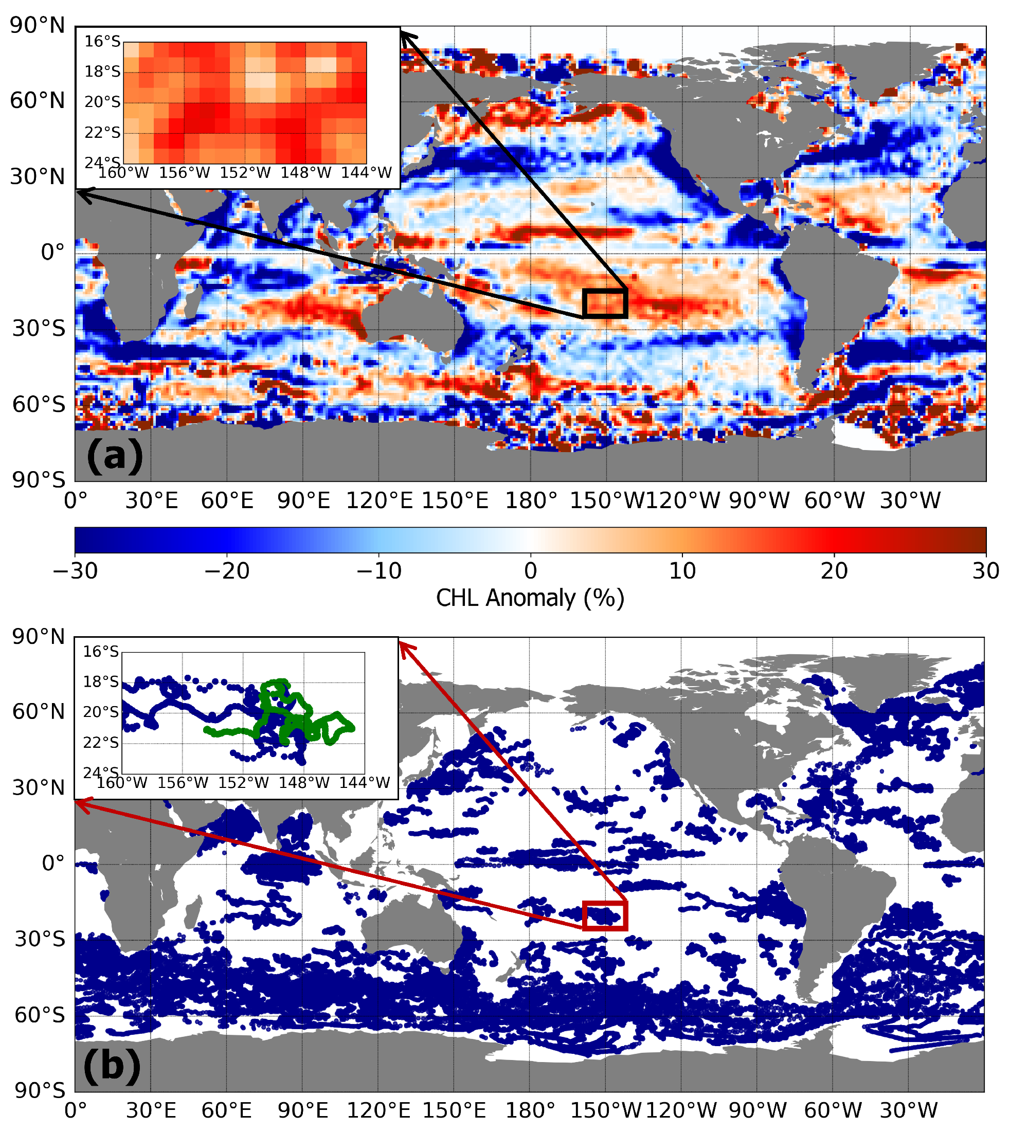
3.1. Chlorophyll Characteristics of Sea Surface

We first derived the distribution of global sea surface Chl anomalies through analysis of remote sensing data (Figure 1a). The concentration of Chl in AEs is higher than that in CEs in subtropical gyres, such as the SPO and the South Indian Ocean (SIO), and the opposite is the case with mid-latitude oceans and areas of boundary currents. To study this anomaly in sea surface and subsurface Chl characteristics, a specific area (16°S–24°S, 160°W–144°W) was selected and used to represent the SPO. In this region, the Chl′ > 0 at each 1° × 1° grid ensured the stability of Chl anomalies in this region, and the mean value peaked at 11.6%. There were hundreds of biochemical profiles containing Chl, BBP, nitrate, temperature, and light data in the selected area (Figure 1b), providing the possibility of studying Chl profile characteristics and environmental factors in this area.

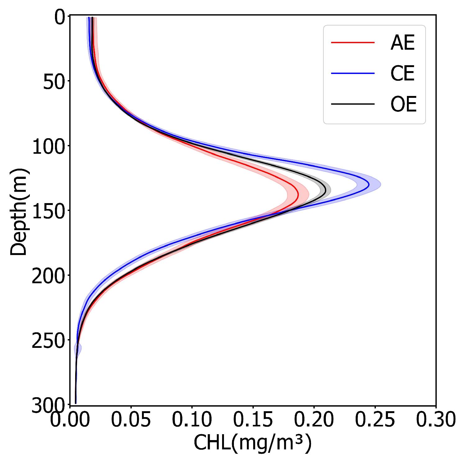
3.2. Subsurface Chlorophyll Structure in Eddies

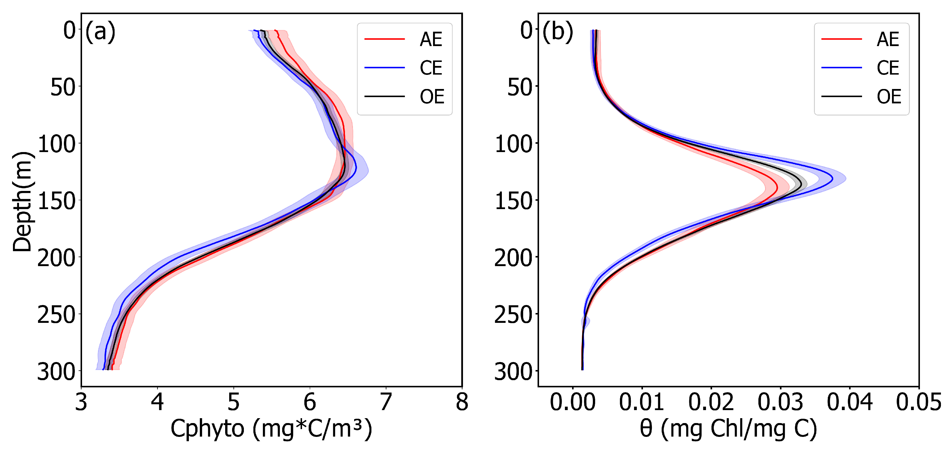
We retained 1028 biochemical profiles in the selected area. About 147 profiles were located in 41 CEs and 138 profiles in 43 AEs. All these profiles contained Chl, BBP, temperature, and PAR data, while the nitrate data were slightly less. In this study, we categorized the Chl profile into three distinct water layers: the MLD, the intermediate layer spanning from 50 m to 150 m (the middle layer was further divided into two sub-layers, one ranging from 50 m to 110 m and the other from 110 m to 150 m near the pycnocline, which encompassed the SCM), and the deep layer situated below 150 m. Then, we calculated the depth of the mixed layer, ZEU, and subsurface chlorophyll maximum depth (SCMD) (

Table 1. MLD, ZEU, and SCMD in eddies of different polarity.

	AE	CE	OE
MLD (m)	51 ± 0.73	40 ± 0.65	44 ± 0.59
ZEU (m)	126.4 ± 0.27	125.1 ± 0.25	126.6 ± 0.36
SCMD (m)	139 ± 0.76	131 ± 0.67	135 ± 0.49

), and the Chl′, CPhyto′, θ′, Temperature′, PAR′, Nitrate′, and SCM′ within the corresponding layer (

Table 2. Anomaly of Chl, CPhyto, $\theta$, temperature, PAR, and nitrate at different levels, calculated by BGC-Argo data.

Depth	Chl′	CPhyto′	θ′	Temp′	PAR′	Nitrate′
0-MLD	21% ± 2.9%	5.1% ± 1.1%	15.6% ± 1.8%	2.2% ± 0.2%	−6.3% ± 0.1%	65% ± 19.1%
50–110 m	−7.9% ± 0.5%	1.7% ± 0.4%	−9.2% ± 1.2%	3.9% ± 0.3%	6.1% ± 0.7%	35.8% ± 16.5%
110–150 m	−25% ± 1.3%	−1.2% ± 0.3%	−23.6% ± 2.5%	4.5% ± 0.1%	9.9% ± 3.2%	−10% ± 3.6%
150–300 m	12.6% ± 1.7%	4.1% ± 0.9%		4.5% ± 0.2%	5.8% ± 1.5%	−5.4% ± 0.3%
SCM	−27.7% ± 3.2%

) were also calculated. In order to better observe the differences of these vertical profile data in AEs, CEs, and OE, we also provided a supporting information document, which included enlarged images of the vertical distribution of Chl, Cphyto, $\theta$, nitrate, PAR, and temperature in AEs, CEs, and OE at different depths.

Within the mixed layer, the Chl concentration in the AEs was slightly higher than that in the CEs (Figure 2, Table 1), and the Chl′ = 21% was higher than the result of the remote sensing data. At the depths of 50–150 m in the middle layer the Chl concentration increased rapidly with depth and the Chl concentration of the CEs was significantly higher than that of the AEs, which was inconsistent with the results for the mixed layer and remote sensing. At the bottom of the middle layer (110–150 m) the SCM feature appeared, and the relative ratio of the Chl within the AEs and the CEs reached its maximum (SCM′ = −27.7%). Furthermore, the application of AEs resulted in a deepening of the SCMD, while CEs shallowed it ($SCM{D}_{AE}=139$ m, $SCM{D}_{CE}=131$ m, $SCM{D}_{OE}=135$ m). At a depth of 150 m from the sea surface there was a rapid decline in Chl concentration. Meanwhile, the Chl concentration in the AEs was higher than that in the CEs. It is worth mentioning that the depth of 150 m underwater is deeper than the ZEU, rendering it essentially in a state of “almost complete darkness” and unsuitable for phytoplankton growth. Therefore, the Chl synthesis signal was gradually attenuated, leading to a decline in biomass and a rapid reduction in Chl concentration.

In general, both phytoplankton biomass and physiological adaptations in cellular pigmentation can affect Chl concentrations [41]. Therefore, to gain a comprehensive understanding of Chl profile characteristics, CPhyto data and $\theta$ data needed to be studied.

3.3. CPhyto and $\theta$

To quantify the relationship between phytoplankton biomass, physiological adjustment and Chl, CPhyto and $\theta$ profiles were examined, using BGC-Argo data (Figure 3). The CPhyto profile data depicted the biomass distribution influenced by the AEs/CEs within the ocean’s interior (Figure 3a); $\theta$ means the concentration of pigment in phytoplankton cells (Figure 3b), and it reflects the strength of the physiological adjustment ability of phytoplankton. An increase of $\theta$ indicates a proportional rise in the concentration of Chl within the phytoplankton cell. Similar to the Chl profile, CPhyto and $\theta$ also showed a trend of first increasing and then decreasing with increasing depth. This reflected that the Chl concentration was influenced by both the physiological adjustment and biomass of the phytoplankton.

In the mixed layer, the concentration of CPhyto in the AEs was found to be higher than in the CEs, which was consistent with the Chl results. The Chl′ = 21% and the CPhyto′ = 5.1% in the mixed layer, which suggested that although the Chl in the AEs was much higher than in the CEs, the biomass was not significantly higher (Figure 3, Table 1). The $\theta$ profile precisely explains this phenomenon: θ′ = 15.6% in this layer, indicating that the pigment concentration per individual phytoplankton cell in the AEs was higher than in the CEs. That is, in the mixed layer, the higher Chl concentration in the AEs compared to the CEs was driven by both the biomass and the physiological adjustment of the phytoplankton, and it induced a higher concentration of Chl′ than CPhyto′.

Within the middle layer of 50–110 m, the concentration of CPhyto in the AEs was higher than in the CEs (CPhyto′ = 1.7%), whereas the Chl concentration in the AEs was lower (Chl′ = −7.97%). This observation suggests that increased CPhyto concentration in AEs does not lead to a higher Chl concentration compared to CEs at this layer, whereas the physiological adjustment of the phytoplankton was the primary factor contributing to the lower Chl concentration in the AEs compared to the CEs (θ′ = −9.2%), and the biomass hindered this process. At 110–150 m, the CPhyto concentration and $\theta$ in the CEs were higher than those in the AEs (CPhyto′ = −1.2%, θ′ = −23.6%). Biomass and the capacity for physiological adaptation also peaked in this layer (Figure 2 and Figure 3). The higher Chl within the CEs compared to the AEs can be attributed to the synergistic effect of enhanced biomass and physiological regulation in CEs.

At depths of 150 m and deeper, the CPhyto content was higher in the AEs than in the CEs, which was consistent with the Chl results (CPhyto′ = 4.1%, Chl′ = 12.6%). Below a 150 m water layer, light is extremely weak or absent, and it is unsuitable for photosynthesis in phytoplankton. Therefore, the physiological adjustment of phytoplankton was not within the scope of discussion in this study at this layer, and the higher Chl concentration within the AEs compared to the CEs was determined by biomass.

In conclusion, Chl concentration is influenced by biomass and by the physiological adjustment of phytoplankton, and these cannot simply be lumped together. The contribution of biomass and the physiological adjustments of phytoplankton to chlorophyll concentration vary at different depths.

4. Discussion

To further understand the mechanism of Chl anomalies, we analyzed how eddies modulate biomass and physiological adjustment through regulating nitrates, temperature, and light and, ultimately, how this influences Chl concentration, using biochemical data. In general, nitrate concentration is essential for phytoplankton growth [42]. Our study also illustrated that the nitrate and CPhyto profiles exhibited high correlations: both the nitrate concentration and the CPhyto in the AEs was higher than in the CEs in the ZEU (Figure 3a and Figure 4c, Table 2). And with the rapid decline of phytoplankton biomass, the nitrate concentration increased rapidly at around 150 m, due to the reduced consumption of nitrates (Figure 3a and Figure 4c). While temperature and light tend to affect both physiological regulation and phytoplankton growth, lower temperature and light can promote Chl synthesis in phytoplankton cells [3,4,6,43].

In the mixed layer, our research shows that higher Chl concentration in AEs compared to CEs is driven by both biomass and the physiological adjustment of phytoplankton. Whether biomass or pigment concentration is responsible for the difference in Chl concentration between AEs and CEs is ultimately determined by the influence of eddies on nutrients, temperature, and light [44]. From the perspective of phytoplankton biomass, both nitrate and temperature play crucial roles in determining biomass under optimal light conditions for phytoplankton growth [45]. On the one hand, due to the modulation mechanism of the eddies on the MLD (AEs deepen the MLD while CEs make it shallower) AEs can contact more nutrient from the bottom of the mixed layer [19,46,47,48], and the turbulent mixing enables AEs to have higher nutrient concentrations and promotes phytoplankton growth (Figure 3a and Figure 4c, Table 1). On the other hand, because of the function of the eddy pump, AEs have a higher temperature relative to CEs (Figure 4a) (temperature′ = 2.2%), and the higher temperature in the AEs promotes the metabolic capacity of the phytoplankton, which promotes the growth of the phytoplankton, increasing the biomass [49]. So, the increase in Chl resulting from the rise in biomass is attributable to the synergistic effects of elevated nitrate levels and temperature in AEs. Certainly, in addition to biomass, the physiological adaptation of phytoplankton that is induced by temperature and light is also a major factor affecting chlorophyll concentration. The higher temperature will reduce the concentration of pigment in phytoplankton cells [6], and it will finally weaken the Chl concentration within AEs, making the Chl′ lower than the CPhyto′. However, the opposite situation has emerged currently: our findings indicate that the Chl′ is higher than the CPhyto′ in the mixed layer (Table 1). This suggests that temperature may not be the primary determinant influencing phytoplankton’s physiological adjustment in the mixed layer: although the higher temperature can reduce the concentration of pigment in phytoplankton cells in AEs, the lower light makes it higher, ultimately [50]. The deepened MLD in AEs increases the vertical migration of subsurface phytoplankton, resulting in a reduction in light exposure and, thus, contributing to an increase in cellular pigment, due to light adaption [21]. Therefore, in the mixed layer of the SPO, we inferred that the biomass and phytoplankton photo-adaptation together caused higher chlorophyll concentrations in the AEs than in the CEs and that the dominant role in this process was played by phytoplankton light adaptation, as the Chl′ was three times larger than the CPhyto′ (Table 2).

At depths of 50–110 m in the middle layer, the difference in chlorophyll concentration between AEs and CEs was reversed compared to the mixed layer (Chl′ = −7.97%), and CPhyto′ was down to 1.7%. Although the higher nutrient concentration in the AEs resulted in the increased biomass and chlorophyll concentration of the phytoplankton (Nitrate′ = 35.8%), indicating a positive response to nutrient enrichment (Figure 3a and Figure 4c), the light was weakened as the water depth increased. The physiological adjustment ability of the phytoplankton also gradually increased [6,23] and, finally, became the main factor, dominating the Chl concentration (Figure 3b and Figure 4b). At the same time, the lower temperature in the CEs promoted higher Chl in the CEs compared to the AEs. Therefore, the Chl concentration in the CEs was higher than that in the AEs, mainly due to the higher physiological adjustment ability induced by the lower light and temperature of the phytoplankton in the CEs compared to the AEs, while the slightly higher biomass in the AEs did not change the process.

The depth of 110–150 m in the middle layer was a special location: the bottom of the ZEU and SCM/SCMD appeared here (Table 2, Figure 2 and Figure 4). The biomass and Chl concentration in the AEs were lower than in the CEs, which was the opposite case to that of the mixed layer, and the absolute value of the Chl′ was greater than the CPhyto′ (CPhyto′ = −1.2%, Chl′ = −25%). At this water layer, the light intensity further diminishes and tends to be negligible at the bottom of the ZEU, and the light adaptation of the phytoplankton is enhanced to a peak [26,51]. Phytoplankton physiological regulation has a strong influence on Chl concentration: even subtle differences between AEs and CEs can lead to significant variations in Chl levels at the bottom of the ZEU [6]. Thus, it can be observed that the differences in nitrate concentration, temperature, and biomass between the AEs and CEs near the bottom of the ZEU remained relatively stable compared to those in the mixed layer, while variations in the Chl concentration were maximized (Figure 2 and Figure 4). On the other hand, the convergence and subsidence of the AEs and the divergence and uplift of the CEs near the SCM resulted in the phytoplankton in the AEs being transported to deeper layers, leading to a dilution effect on the biomass. Conversely, the phytoplankton in the CEs was enriched, due to the uplifting, resulting in slightly higher biomass and Chl concentration compared with the AEs [26]. Therefore, the higher Chl concentration in the CEs was due to both an increase in biomass and higher pigment concentrations within the phytoplankton cells as a result of physiological adjustment and to the physiological adjustment induced by lower illumination playing a dominant role (CPhyto′ = −1.2%, Chl′ = −25%, θ′ = −23.6%).

Below the 150 m water layer, the Chl and biomass concentration within the AEs/CEs/OE decreased sharply, whereas the concentration of nutrients, in contrast, exhibited a significant increase (Figure 4c). A possible mechanism may be that below the depth of the ZEU and the SCM (the SCM generally occurs under the ZEU) the light was too weak or there was no light to allow phytoplankton to photosynthesize, which meant that the Chl synthesis was ‘off’ and caused a sharp reduction in biomass [6]. Also, the nitrate concentration dramatically increased in the absence of phytoplankton depletion [45,52]. Meanwhile, the downwelling sank down the phytoplankton in the AEs, and the upwelling in the CEs uplifted it, which resulted in Chl concentration and biomass higher in the AEs compared to the CEs [10].

On the whole, the phytoplankton biomass in the AEs was higher than in the CEs in the SPO (Table 1), which is consistent with previous research [19]. Recent research has shown that anticyclonic eddies aggregate pelagic predators in subtropical gyres [53]. This may be due to the fact that the increased phytoplankton volume in the AEs feeds more zooplankton and then attracts more predators. This also attests to the validity of this study from another perspective.

Additionally, the eddy pump enables CEs to transport substances such as nutrients from the deep to the shallows of the ocean, thereby facilitating phytoplankton growth. Conversely, AEs have an opposite effect. However, it has been observed that the Chl concentration, biomass, and nutrient in AEs exceed those found in CEs within the mixed layer in this region, which contradicts the traditional assumption based on eddy pumping. The reason may be that in the subtropical gyres region the eddy kinetic energy is weak [9] and that the capacity of marine stratification is stronger than in other regions. Therefore, it is difficult for CEs to carry the eutrophic water to the surface from the deep ocean through eddy pumping; however, AEs can contact more nutrients because of the deepening MLD and promote the growth of phytoplankton. This may be one of the reasons for the higher Chl concentration in AEs compared to CEs in subtropical gyres, such as the SPO and the SIO, as presented by current satellite remote sensing results.

5. Conclusions

In this study, we were the first to address the effect of mesoscale eddies on Chl profile anomalies at different depths in parts of the SPO, using remote sensing and BGC-Argo data, and we explained the mechanism of the Chl anomaly in a previous study that mainly used remote sensing data. The eddy-induced biochemical cycle is a complex process: the Chl and biomass of the phytoplankton interact with various environmental factors and adapt to each other. A single model cannot perfectly explain the characteristics of Chl and biomass distribution and the capability of primary productivity at different depths in the ocean [6]. Therefore, stratifying the ecological effects induced by eddies according to different depths provided a new idea for the assessment of marine primary productivity and biogeochemical processes under the influence of eddies.

Firstly, whether Chl concentration was influenced dominantly by biomass or by physiological adjustment was analyzed in conjunction with the profile characteristics of CPhyto and $\theta$ in the region. Then, we further analyzed how mesoscale eddies regulate biomass, physiological processes and, thus, Chl distribution by affecting nutrients, temperature, and light, using nitrate, temperature, and PAR data. The results showed that the nutrients, temperature, and light all had an effect on phytoplankton biomass and physiological adjustment, and they each had their own focus among different depths of water column.

The main findings were as follows:

(1) In mixed layer, AEs have a higher Chl concentration than CEs, driven by both biomass and the physiological adjustment of the phytoplankton, and the physiological adjustment plays a predominant role. As a result of the convergent subsidence, AEs deepen the MLD and can contact deeper nutrient lines, and the mixing of turbulent flow enables AEs to have higher nutrient concentrations and promotes phytoplankton growth. The deepening MLD in AEs increases the vertical migration of subsurface phytoplankton, resulting in a reduction in light exposure and, thus, contributing to an increase in cellular pigment due to light adaption, and the higher temperature in AEs makes a small negative contribution.

(2) At depths of 50–110 m, the Chl concentration in CEs is higher than in AEs, mainly because the light is weakened with the increase of depth, which enhances the physiological adjustment ability of the phytoplankton, which then becomes the dominant factor affecting the Chl concentration. The lower temperature and light in CEs promotes the increase of pigment in phytoplankton cells.

(3) Near the SCM at 110–150 m, CEs have higher Chl concentration than AEs, due to an increase in biomass in the CEs, on the one hand, and physiological effects, on the other. The lower temperature and light in CEs increases pigmentation in phytoplankton cells and plays a predominant role in Chl concentration, and the upwelling in the CEs causes phytoplankton to rise and accumulate there. Both of these promote a higher Chl concentration in CEs at this layer, resulting in a stronger SCM and a shallower SCMD in CEs.

(4) Below a 150 m water layer, the light is too weak to allow phytoplankton to photosynthesize, and both pigment concentration in phytoplankton and biomass decrease sharply. The higher concentration of Chl in AEs compared to CEs is mainly due to the sedimentation of phytoplankton caused by downwelling in AEs, while CEs play an opposite role.

Naturally, our current study does possess certain limitations: the restricted number of BGC-Argo samples resulted in marginally diminished data precision, and the available dataset was insufficient to adequately support an investigation into Chl variations attributed to seasonal fluctuations and other influencing factors. Furthermore, the Chl concentration induced by the central and peripheral regions of eddies exhibited dissimilar patterns, and our current dataset was insufficient for their comprehensive analysis. In the future, with the increasing of BGC-Argo profile numbers, we will conduct seasonal and quantitative analyses of environmental factors affecting Chl concentrations and biomass. The difference in Chl between the center and edge of the mesoscale eddies will be studied, the three-dimensional ecological structure of mesoscale eddies and its modulation mechanism will also be part of our research, and the research results will be more reliable. Our study will significantly contribute to the understanding of eddy-induced biogeochemical processes.

References

1. Field, C.B.; Behrenfeld, M.J.; Randerson, J.T.; Falkowski, P. Primary production of the biosphere: Integrating terrestrial and oceanic components. Science 1998, 281, 237–240. [Google Scholar] [CrossRef]
2. Chassot, E.; Bonhommeau, S.; Dulvy, N.K.; Mélin, F.; Watson, R.; Gascuel, D.; Le Pape, O. Global marine primary production constrains fisheries catches. Ecol. Lett. 2010, 13, 495–505. [Google Scholar] [CrossRef] [PubMed]
3. Feng, J.; Durant, J.M.; Stige, L.C.; Hessen, D.O.; Hjermann, D.Ø.; Zhu, L.; Llope, M.; Stenseth, N.C. Contrasting correlation patterns between environmental factors and chlorophyll levels in the global ocean. Glob. Biogeochem. Cycles 2015, 29, 2095–2107. [Google Scholar] [CrossRef]
4. Zhao, D.; Gao, L.; Xu, Y. Quantification of the impact of environmental factors on chlorophyll in the open ocean. J. Oceanol. Limnol. 2021, 39, 447–457. [Google Scholar] [CrossRef]
5. Halsey, K.H.; Jones, B.M. Phytoplankton strategies for photosynthetic energy allocation. Annu. Rev. Mar. Sci. 2015, 7, 265–297. [Google Scholar] [CrossRef] [PubMed]
6. Behrenfeld, M.J.; O’Malley, R.T.; Boss, E.S.; Westberry, T.K.; Graff, J.R.; Halsey, K.H.; Milligan, A.J.; Siegel, D.A.; Brown, M.B. Revaluating ocean warming impacts on global phytoplankton. Nat. Clim. Chang. 2016, 6, 323–330. [Google Scholar] [CrossRef]
7. Chelton, D.B.; Schlax, M.G.; Samelson, R.M. Global observations of nonlinear mesoscale eddies. Prog. Oceanogr. 2011, 91, 167–216. [Google Scholar] [CrossRef]
8. He, Q.; Zhan, H.; Cai, S.; He, Y.; Huang, G.; Zhan, W. A new assessment of mesoscale eddies in the South China Sea: Surface features, three-dimensional structures, and thermohaline transports. J. Geophys. Res. Ocean. 2018, 123, 4906–4929. [Google Scholar] [CrossRef]
9. Chen, G.; Han, G. Contrasting short-lived with long-lived mesoscale eddies in the global ocean. J. Geophys. Res. Ocean. 2019, 124, 3149–3167. [Google Scholar] [CrossRef]
10. Chelton, D.B.; Gaube, P.; Schlax, M.G.; Early, J.J.; Samelson, R.M. The influence of nonlinear mesoscale eddies on near-surface oceanic chlorophyll. Science 2011, 334, 328–332. [Google Scholar] [CrossRef]
11. Batten, S.D.; Crawford, W.R. The influence of coastal origin eddies on oceanic plankton distributions in the eastern Gulf of Alaska. Deep. Sea Res. Part II Top. Stud. Oceanogr. 2005, 52, 991–1009. [Google Scholar] [CrossRef]
12. Conway, T.M.; Palter, J.B.; de Souza, G.F. Gulf Stream rings as a source of iron to the North Atlantic subtropical gyre. Nat. Geosci. 2018, 11, 594–598. [Google Scholar] [CrossRef]
13. Xu, G.; Dong, C.; Liu, Y.; Gaube, P.; Yang, J. Chlorophyll rings around ocean eddies in the North Pacific. Sci. Rep. 2019, 9, 2056. [Google Scholar] [CrossRef]
14. Liu, Y.; Li, X.; Ren, Y. A deep learning model for oceanic mesoscale eddy detection based on multi-source remote sensing imagery. In Proceedings of the IGARSS 2020—2020 IEEE International Geoscience and Remote Sensing Symposium, Virtual, 26 September–2 October 2020; IEEE: Piscataway, NJ, USA, 2020; pp. 6762–6765. [Google Scholar]
15. Xing, Q.; Yu, H.; Wang, H.; Ito, S.I.; Chai, F. Mesoscale eddies modulate the dynamics of human fishing activities in the global midlatitude ocean. Fish Fish. 2023, 24, 527–543. [Google Scholar] [CrossRef]
16. Dawson, H.R.; Strutton, P.G.; Gaube, P. The unusual surface chlorophyll signatures of Southern Ocean eddies. J. Geophys. Res. Ocean. 2018, 123, 6053–6069. [Google Scholar] [CrossRef]
17. McGillicuddy, D.J., Jr. Mechanisms of physical-biological-biogeochemical interaction at the oceanic mesoscale. Annu. Rev. Mar. Sci. 2016, 8, 125–159. [Google Scholar] [CrossRef]
18. Gaube, P.; Chelton, D.B.; Strutton, P.G.; Behrenfeld, M.J. Satellite observations of chlorophyll, phytoplankton biomass, and Ekman pumping in nonlinear mesoscale eddies. J. Geophys. Res. Ocean. 2013, 118, 6349–6370. [Google Scholar] [CrossRef]
19. Dufois, F.; Hardman-Mountford, N.J.; Greenwood, J.; Richardson, A.J.; Feng, M.; Matear, R.J. Anticyclonic eddies are more productive than cyclonic eddies in subtropical gyres because of winter mixing. Sci. Adv. 2016, 2, e1600282. [Google Scholar] [CrossRef]
20. Arteaga, L.; Pahlow, M.; Oschlies, A. Modeled Chl: C ratio and derived estimates of phytoplankton carbon biomass and its contribution to total particulate organic carbon in the global surface ocean. Glob. Biogeochem. Cycles 2016, 30, 1791–1810. [Google Scholar] [CrossRef]
21. He, Q.; Zhan, H.; Cai, S.; Zhan, W. Eddy-induced near-surface chlorophyll anomalies in the subtropical gyres: Biomass or physiology? Geophys. Res. Lett. 2021, 48, e2020GL091975. [Google Scholar] [CrossRef]
22. Gordon, H.R.; McCluney, W. Estimation of the depth of sunlight penetration in the sea for remote sensing. Appl. Opt. 1975, 14, 413–416. [Google Scholar] [CrossRef]
23. Cornec, M.; Claustre, H.; Mignot, A.; Guidi, L.; Lacour, L.; Poteau, A.; d’Ortenzio, F.; Gentili, B.; Schmechtig, C. Deep chlorophyll maxima in the global ocean: Occurrences, drivers and characteristics. Glob. Biogeochem. Cycles 2021, 35, e2020GB006759. [Google Scholar] [CrossRef] [PubMed]
24. Letelier, R.M.; Karl, D.M.; Abbott, M.R.; Flament, P.; Freilich, M.; Lukas, R.; Strub, T. Role of late winter mesoscale events in the biogeochemical variability of the upper water column of the North Pacific Subtropical Gyre. J. Geophys. Res. Ocean. 2000, 105, 28723–28739. [Google Scholar] [CrossRef]
25. Cullen, J.J. Subsurface chlorophyll maximum layers: Enduring enigma or mystery solved? Annu. Rev. Mar. Sci. 2015, 7, 207–239. [Google Scholar] [CrossRef] [PubMed]
26. Cornec, M.; Laxenaire, R.; Speich, S.; Claustre, H. Impact of mesoscale eddies on deep chlorophyll maxima. Geophys. Res. Lett. 2021, 48, e2021GL093470. [Google Scholar] [CrossRef] [PubMed]
27. Schlax, M.G.; Chelton, D.B. The “Growing Method” of Eddy Identification and Tracking in Two and Three Dimensions; College of Earth, Ocean and Atmospheric Sciences, Oregon State University: Corvallis, OR, USA, 2016; Volume 8, p. 23. [Google Scholar]
28. Peng, L.; Chen, G.; Guan, L.; Tian, F. Contrasting westward and eastward propagating mesoscale eddies in the global ocean. IEEE Trans. Geosci. Remote Sens. 2021, 60, 4504710. [Google Scholar] [CrossRef]
29. Wong, A.P.; Wijffels, S.E.; Riser, S.C.; Pouliquen, S.; Hosoda, S.; Roemmich, D.; Gilson, J.; Johnson, G.C.; Martini, K.; Murphy, D.J.; et al. Argo data 1999–2019: Two million temperature-salinity profiles and subsurface velocity observations from a global array of profiling floats. Front. Mar. Sci. 2020, 7, 700. [Google Scholar] [CrossRef]
30. Johnson, K.; Claustre, H. The scientific rationale, design and Implementation Plan for a Biogeochemical-Argo float array. Biogeochem.-Argo Plan. Group 2016, 58, 46601. [Google Scholar]
31. Bittig, H.C.; Maurer, T.L.; Plant, J.N.; Schmechtig, C.; Wong, A.P.; Claustre, H.; Trull, T.W.; Udaya Bhaskar, T.; Boss, E.; Dall’Olmo, G.; et al. A BGC-Argo guide: Planning, deployment, data handling and usage. Front. Mar. Sci. 2019, 6, 502. [Google Scholar] [CrossRef]
32. Sukigara, C.; Inoue, R.; Sato, K.; Mino, Y.; Nagai, T.; Fassbender, A.J.; Takeshita, Y.; Bishop, S.; Oka, E. Observing intermittent biological productivity and vertical carbon transports during the spring transition with BGC Argo floats in the western North Pacific. Biogeosci. Discuss. 2022, 2022, 1–52. [Google Scholar]
33. Xing, X.; Claustre, H.; Uitz, J.; Mignot, A.; Poteau, A.; Wang, H. Seasonal variations of bio-optical properties and their interrelationships observed by B io-A rgo floats in the subpolar N orth A tlantic. J. Geophys. Res. Ocean. 2014, 119, 7372–7388. [Google Scholar] [CrossRef]
34. Chai, F.; Johnson, K.S.; Claustre, H.; Xing, X.; Wang, Y.; Boss, E.; Riser, S.; Fennel, K.; Schofield, O.; Sutton, A. Monitoring ocean biogeochemistry with autonomous platforms. Nat. Rev. Earth Environ. 2020, 1, 315–326. [Google Scholar] [CrossRef]
35. de Boyer Montégut, C.; Madec, G.; Fischer, A.S.; Lazar, A.; Iudicone, D. Mixed layer depth over the global ocean: An examination of profile data and a profile-based climatology. J. Geophys. Res. Ocean. 2004, 109. [Google Scholar] [CrossRef]
36. Wang, Y.; Yang, J.; Chen, G. Euphotic Zone Depth Anomaly in Global Mesoscale Eddies by Multi-Mission Fusion Data. Remote Sens. 2023, 15, 1062. [Google Scholar] [CrossRef]
37. Oubelkheir, K. Biogeochemical Characterization of Various Oceanic Provinces through Optical Indicators over Various Space and Time Scales. Ph.D. Thesis, Université de la Méditerraneé/CNRS, Marseille, France, 2001; p. 216. [Google Scholar]
38. Behrenfeld, M.J.; Boss, E.; Siegel, D.A.; Shea, D.M. Carbon-based ocean productivity and phytoplankton physiology from space. Glob. Biogeochem. Cycles 2005, 19. [Google Scholar] [CrossRef]
39. Stramski, D.; Reynolds, R.A.; Babin, M.; Kaczmarek, S.; Lewis, M.R.; Röttgers, R.; Sciandra, A.; Stramska, M.; Twardowski, M.; Franz, B.; et al. Relationships between the surface concentration of particulate organic carbon and optical properties in the eastern South Pacific and eastern Atlantic Oceans. Biogeosciences 2008, 5, 171–201. [Google Scholar] [CrossRef]
40. Xing, X.; Wells, M.L.; Chen, S.; Lin, S.; Chai, F. Enhanced winter carbon export observed by BGC-Argo in the Northwest Pacific Ocean. Geophys. Res. Lett. 2020, 47, e2020GL089847. [Google Scholar] [CrossRef]
41. Kerimoglu, O.; Hofmeister, R.; Maerz, J.; Riethmüller, R.; Wirtz, K.W. The acclimative biogeochemical model of the southern North Sea. Biogeosciences 2017, 14, 4499–4531. [Google Scholar] [CrossRef]
42. Martin, A.; Pondaven, P. On estimates for the vertical nitrate flux due to eddy pumping. J. Geophys. Res. Ocean. 2003, 108. [Google Scholar] [CrossRef]
43. Gregg, W.W.; Casey, N.W.; McClain, C.R. Recent trends in global ocean chlorophyll. Geophys. Res. Lett. 2005, 32. [Google Scholar] [CrossRef]
44. Poppeschi, C.; Charria, G.; Daniel, A.; Verney, R.; Rimmelin-Maury, P.; Retho, M.; Goberville, E.; Grossteffan, E.; Plus, M. Interannual variability of the initiation of the phytoplankton growing period in two French coastal ecosystems. Biogeosciences Discuss. 2022, 2022, 5667–5687. [Google Scholar] [CrossRef]
45. Wu, M.L.; Wang, Y.S.; Wang, Y.T.; Yin, J.P.; Dong, J.D.; Jiang, Z.Y.; Sun, F.L. Scenarios of nutrient alterations and responses of phytoplankton in a changing Daya Bay, South China Sea. J. Mar. Syst. 2017, 165, 1–12. [Google Scholar] [CrossRef]
46. He, Q.; Zhan, H.; Shuai, Y.; Cai, S.; Li, Q.P.; Huang, G.; Li, J. Phytoplankton bloom triggered by an anticyclonic eddy: The combined effect of eddy-E kman pumping and winter mixing. J. Geophys. Res. Ocean. 2017, 122, 4886–4901. [Google Scholar] [CrossRef]
47. Wang, T.; Ning, J.; Xu, Q. The Enhancement of Upper Ocean Nutrients Concentration in the Peripheries of Two Anti-Cyclonic Eddies. In Proceedings of the IGARSS 2018—2018 IEEE International Geoscience and Remote Sensing Symposium, Valencia, Spain, 22–27 July 2018; IEEE: Piscataway, NJ, USA, 2018; pp. 7624–7627. [Google Scholar]
48. Gaube, P.; McGillicuddy, D.J., Jr.; Moulin, A.J. Mesoscale eddies modulate mixed layer depth globally. Geophys. Res. Lett. 2019, 46, 1505–1512. [Google Scholar] [CrossRef]
49. Behrenfeld, M.J.; Boss, E.S. Resurrecting the ecological underpinnings of ocean plankton blooms. Annu. Rev. Mar. Sci. 2014, 6, 167–194. [Google Scholar] [CrossRef] [PubMed]
50. Geider, R.J. Light and temperature dependence of the carbon to chlorophyll a ratio in microalgae and cyanobacteria: Implications for physiology and growth of phytoplankton. New Phytol. 1987, 106, 1–34. [Google Scholar] [CrossRef]
51. Behrenfeld, M.J.; Halsey, K.H.; Milligan, A.J. Evolved physiological responses of phytoplankton to their integrated growth environment. Philos. Trans. R. Soc. Biol. Sci. 2008, 363, 2687–2703. [Google Scholar] [CrossRef] [PubMed]
52. d’Ortenzio, F.; Taillandier, V.; Claustre, H.; Coppola, L.; Conan, P.; Dumas, F.; Durrieu du Madron, X.; Fourrier, M.; Gogou, A.; Karageorgis, A.; et al. BGC-Argo floats observe nitrate injection and spring phytoplankton increase in the surface layer of Levantine Sea (Eastern Mediterranean). Geophys. Res. Lett. 2021, 48, e2020GL091649. [Google Scholar] [CrossRef]
53. Arostegui, M.C.; Gaube, P.; Woodworth-Jefcoats, P.A.; Kobayashi, D.R.; Braun, C.D. Anticyclonic eddies aggregate pelagic predators in a subtropical gyre. Nature 2022, 609, 535–540. [Google Scholar] [CrossRef]
Figure 1. (a) Geographic distributions of eddy-induced Chl anomaly between January 2000 and August 2021. The upper-left subplot displays the distribution of Chl anomalies in the selected area. (b) Map of profiles containing Chl data. In the upper left subplot, the green and blue dots represent the location where BGC-Argo collected data. Each profile of BGC-Argo floats contained Chl, BBP, temperature, and PAR data. The green dots indicate that the profile contained nitrate data, while the blue dots indicate that the profile did not contain nitrate data.
Remotesensing 16 02628 g001
Figure 2. Mean profiles of Chl in eddies of different polarity. Red, blue, and black lines indicate the Chl profile in AEs, CEs, and OE, respectively. Red, blue, and black shadings are 95% confidence intervals for the AEs, CEs, and OE. A zoom of the figure can be seen in Supporting Information Figure S1.
Remotesensing 16 02628 g002
Figure 3. (a,b) Mean profiles of CPhyto and θ (Chl:CPhyto) in eddies of different polarity. Red, blue, and black lines indicate CPhyto and θin AEs, CEs, and OE, respectively. Red, blue, and black shadings are 95% confidence intervals of CPhyto in AEs, CEs, and OE. A zoom of the figure can be seen in Supporting Information Figure S2.
Remotesensing 16 02628 g003
Figure 4. (ac) Profiles of temperature, PAR, and nitrate in eddies of different polarity. Red, blue, and black lines indicate that the profile is for AEs, CEs, and OE, respectively. Red, blue, and black shadings are 95% confidence intervals for AEs, CEs, and OE. A zoom of the figure can be seen in Supporting Information Figures S3–S5.
Remotesensing 16 02628 g004