Utilizing Dual-Stream Encoding and Transformer for Boundary-Aware Agricultural Parcel Extraction in Remote Sensing Images

Abstract

The accurate extraction of agricultural parcels from remote sensing images is crucial for advanced agricultural management and monitoring systems. Existing methods primarily emphasize regional accuracy over boundary quality, often resulting in fragmented outputs due to uniform crop types, diverse agricultural practices, and environmental variations. To address these issues, this paper proposes DSTBA-Net, an end-to-end encoder–decoder architecture. Initially, we introduce a Dual-Stream Feature Extraction (DSFE) mechanism within the encoder, which consists of Residual Blocks and Boundary Feature Guidance (BFG) to separately process image and boundary data. The extracted features are then fused in the Global Feature Fusion Module (GFFM), utilizing Transformer technology to further integrate global and detailed information. In the decoder, we employ Feature Compensation Recovery (FCR) to restore critical information lost during the encoding process. Additionally, the network is optimized using a boundary-aware weighted loss strategy. DSTBA-Net aims to achieve high precision in agricultural parcel segmentation and accurate boundary extraction. To evaluate the model’s effectiveness, we conducted experiments on agricultural parcel extraction in Denmark (Europe) and Shandong (Asia). Both quantitative and qualitative analyses show that DSTBA-Net outperforms comparative methods, offering significant advantages in agricultural parcel extraction.

1. Introduction

Agricultural parcels are fundamental units in agricultural practice and applications [1], serving as the essential material basis for agricultural production and food security [2,3]. The accurate identification and localization of these parcels are critical for crop recognition, yield estimation, and the strategic allocation of agricultural resources [4,5]. In recent years, remote sensing imagery has become the primary tool for extracting agricultural parcels [6,7,8]. While actual parcels can be easily distinguished by clear boundaries formed by physical features such as ditches and roads, the complex spectral, structural, and textural characteristics of land features in remote sensing images present significant challenges for accurate parcel extraction [9,10,11].

Traditional manual methods have enabled the extraction of agricultural parcels [12,13]. These methods can be categorized into three types: edge detection [14,15,16,17,18], region segmentation [19,20,21,22,23,24,25], and machine learning [26,27]. However, these methods are often time-consuming, labor-intensive, and perform poorly in complex scenarios and tasks.

Deep learning, with its ability to automatically learn features, has revolutionized remote sensing applications [28,29,30,31,32,33]. Methods based on Convolutional Neural Networks (CNNs) [34,35,36,37,38,39] and Fully Convolutional Networks (FCNs) [40,41,42,43] have shown great potential. However, spatial diversity results in agricultural parcels having complex shapes and sizes, and remote sensing imagery is often affected by complex backgrounds such as grasslands and bare land. Consequently, existing methods face three main issues: first, difficulty in preserving the unique morphological characteristics of agricultural parcels; second, an inability to ensure the high integrity of extraction results; and third, the challenge of balancing boundary and other detailed morphological features while maintaining high completeness.

To enhance the morphological accuracy of agricultural parcels, some studies have employed instance segmentation and multi-task learning methods. For example, Potlapally et al. [44] utilized Mask R-CNN for instance segmentation, which improved the precision of parcel morphology by independently identifying the boundaries of each parcel. However, these methods exhibit certain limitations when dealing with complex backgrounds and variations in scale. Multi-task learning methods such as ResUNet-a [45] and SEANet [46] have improved morphological accuracy by jointly learning features for different tasks. Nevertheless, these methods often increase the complexity of model training and lack direct task correlations. Although instance segmentation and multi-task learning have somewhat enhanced the morphological accuracy of agricultural parcels, issues such as model complexity, sensitivity to background noise, and reliance on multi-task features result in incomplete extraction outcomes.

To achieve high integrity in segmentation results, some studies have explored constructing networks capable of capturing contextual information using Transformer [47] technology [48,49]. In building extraction, BuildFormer [50] significantly improved the accuracy of building detection by utilizing window-based linear tokens, convolution, MLP, and batch normalization. Chen et al. [51] introduced a dual-channel Transformer framework that achieves more complete building segmentation by leveraging long-distance dependencies in spatial and channel dimensions. Xiao et al. [52] developed the Swin-Transformer with a sliding window mechanism, resulting in more complete segmentation outcomes. Although these methods, primarily based on Transformer networks, have enhanced the completeness of segmentation results to some extent, they face challenges in complex scenes, such as lacking boundary morphology and detailed textures.

To ensure high integrity while preserving certain morphological characteristics, some researchers have begun exploring hybrid models. For instance, Wang et al. [53] integrated Transformer technology into the traditional CNN framework and developed the CCTNet model for barley segmentation in remote sensing images. Xia et al. [54] proposed a Dual-Stream Feature Extraction network that integrates CNN and Transformer technologies to fuse boundary and semantic information, achieving superior results on multiple building datasets. WiCoNet [55] combines CNN and Transformer to fuse global and local information, achieving strong performance on the BLU, GID, and Potsdam remote sensing datasets. STranFuse [56] combines the Swin Transformer with convolutional networks and uses an adaptive fusion module to manage feature representations across different semantic scales, achieving significant performance improvements on the Vaihingen dataset. Wang et al. [57] proposed a dual-stream hybrid structure based on SAM to achieve the fusion of local and global information. However, these combinations of Transformer and CNN typically involve a simple integration of global and local information without specific feature analysis, making it challenging to balance morphological characteristics and segmentation completeness.

Based on the limitations of existing methods in agricultural parcel extraction, this study proposes DSTBA-Net, a segmentation network designed for agricultural parcel extraction. DSTBA-Net processes image and boundary data through Dual-Stream Feature Extraction (DSFE) and effectively fuses these data using a Transformer-dominated Global Feature Fusion Module (GFFM), enhancing boundary morphology and the integrity of extraction results. The decoder employs Feature Compensation Recovery (FCR) to reduce information loss. We propose a boundary-aware weighted loss algorithm to optimize boundary segmentation results. Experimental results demonstrate that DSTBA-Net performs exceptionally well on Danish and Shandong agricultural parcel datasets, exhibiting good generalization ability and robustness.

The main contributions of this study are as follows:

(1)

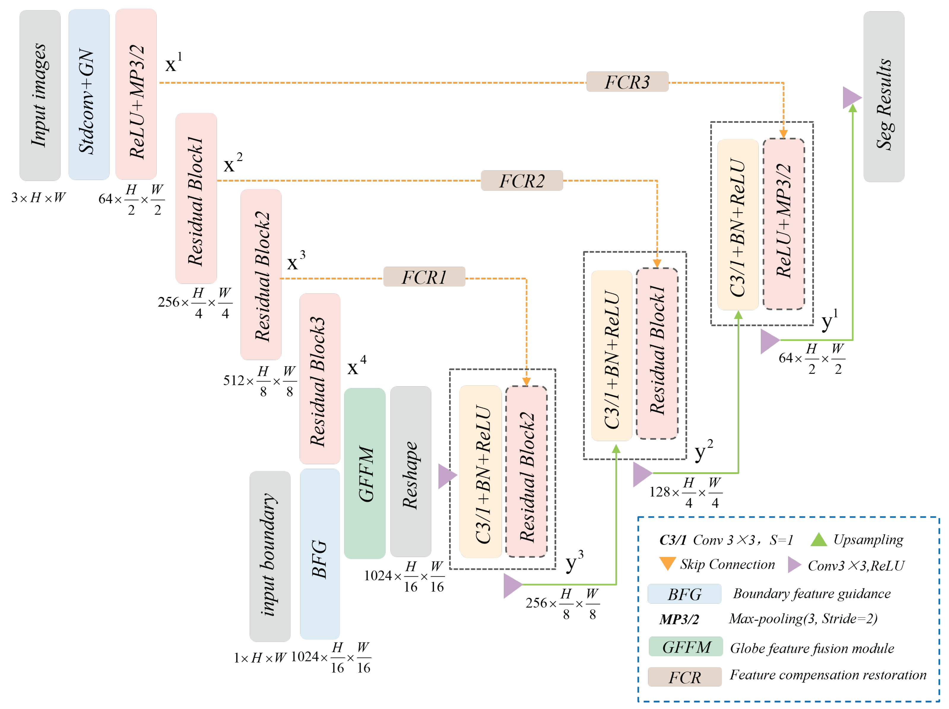
DSTBA-Net, a novel segmentation network framework designed to accurately extract agricultural parcels from remote sensing images, is proposed.

(2)

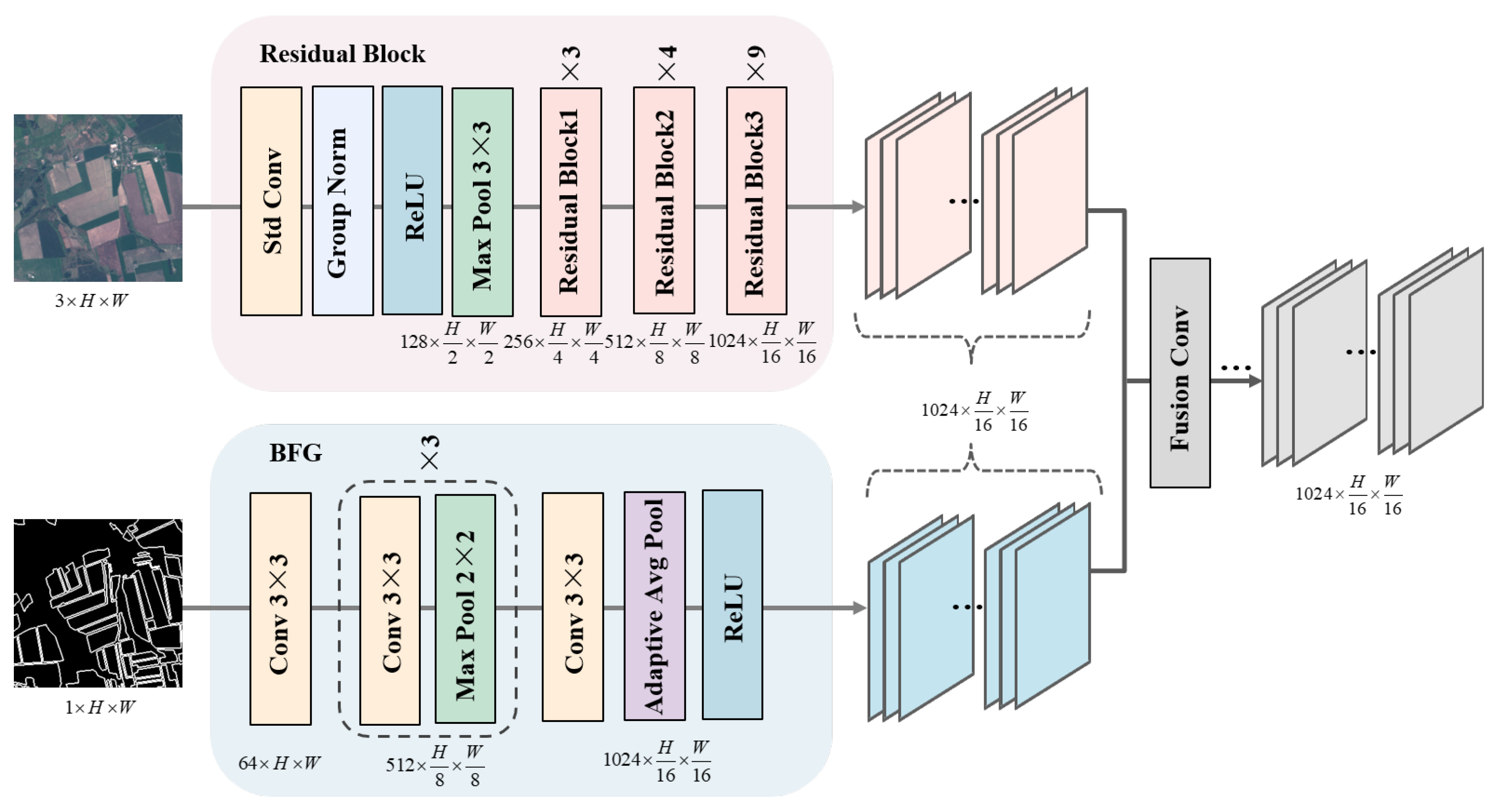
Dual-Stream Feature Extraction (DSFE) is designed to perform multi-level feature extraction on image and boundary data, guiding the model to focus on image edges, thereby preserving the unique morphological characteristics of parcels.

(3)

A Transformer-dominated Global Feature Fusion Module (GFFM) is designed to effectively capture long-distance dependencies and merge them with detailed features, enhancing the completeness of feature extraction.

(4)

A boundary-aware weighted loss algorithm is designed to balance the weights of image interiors and edges, effectively improving feature discrimination.

2. Methodology

This study proposes a semantic segmentation network, termed DSTBA-Net, for extracting agricultural parcels from remote sensing images. The network adopts an encoder–decoder architecture, where the encoder consists of a Dual-Stream Feature Extraction (DSFE) mechanism designed for both image and boundary data, and a Global Feature Fusion Module (GFFM). The decoder achieves accurate upsampling through Feature Compensation Restoration (FCR). Unlike conventional CNN-based algorithms, this study employs a Transformer network to construct the GFFM, facilitating the effective integration of global and detailed information. This approach not only addresses the limitations of using convolutional neural networks alone in handling remote dependencies but also resolves the deficiency of Transformer networks in capturing low-level detail information. The segmentation framework proposed in this study is illustrated in Figure 1.

Additionally, to address challenges arising from boundary imprecision and absence, we propose a boundary-aware weighted loss algorithm. This algorithm incorporates an effective Dice loss function that emphasizes boundary regions. By integrating this function with a weighted binary cross-entropy loss, the network achieves a refined segmentation performance.

2.1. Framework Introduction

The segmentation network framework utilized in this study adopts an end-to-end encoder–decoder architecture. Within this framework, the network processes both image and boundary data simultaneously through a Dual-Stream Feature Extraction (DSFE) mechanism. Image data are processed using an embedded Residual Block to extract complex image features. In contrast, boundary data are captured through an external Boundary Feature Guidance (BFG) mechanism, which flexibly delineates boundary-specific features. Notably, boundary data are obtained using morphological dilation techniques from genuine block labels. Subsequently, in the final segment of the encoder, a meticulously designed Global Feature Fusion Module (GFFM) is employed to construct long-range dependency relationships, facilitating the effective fusion of detailed and global features. To mitigate information loss during the upsampling process, the Feature Compensation Restoration (FCR) technique is applied to accomplish hierarchical upsampling tasks. Furthermore, the model output is refined by utilizing a meticulously crafted boundary-aware weighted loss algorithm, thereby enhancing boundary optimization efforts. The detailed network design is depicted in Figure 2.

In the encoder, as depicted in Figure 3, we have designed a Dual-Stream Feature Extraction (DSFE) mechanism specifically for processing image and boundary data using separate Residual Blocks and Boundary Feature Guidance (BFG).

Specifically, RGB image data with dimensions H and W undergo sequential operations including 7 × 7 convolution, group normalization, ReLU activation, and 3 × 3 max-pooling. Subsequently, an enhanced deep residual network [58] consisting of three blocks, each detailed in Figure 4b, is employed. After being processed by the Residual Blocks, the image feature maps are reduced to 1/16 of the original size in both height and width, with a channel count of 1024, effectively extracting and enhancing high-level image feature representations.

Simultaneously, grayscale boundary data with dimensions H and W undergo a series of operations via BFG, including 3 × 3 convolution, three consecutive 3 × 3 convolutions followed by 2 × 2 max-pooling, a 3 × 3 convolution layer, average pooling, and ReLU activation. The resulting boundary feature maps are also reduced to 1/16 of the original size, with a channel count of 1024. The multiple convolution stages and pooling operations of BFG effectively refine the feature representation of grayscale boundary data, highlighting significant structural elements and spatial relationships within the boundaries. These refinements contribute to achieving precise segmentation and analysis.

Ultimately, through convolution operations, the model captures high-dimensional feature maps that encompass both image texture and boundary information. These feature maps serve as the foundational input for subsequent operations in the Global Feature Fusion Module and decoding section. DSFE integrates the processing requirements of both image and boundary data. By applying Residual Blocks and Boundary Feature Guidance (BFG), the model effectively integrates image and boundary features, significantly enhancing its ability to understand complex scenes and improve segmentation accuracy.

2.2. Global Feature Fusion Module (GFFM)

We propose a Global Feature Fusion Module (GFFM), led by a Transformer, to integrate global contextual information from feature maps containing abundant detailed information; the specific design is shown in Figure 5. Initially, the module captures two classes of features from the image and the boundary through a stacking operation, followed by a series of auxiliary operations to reshape the high-dimensional feature maps into one-dimensional vectors $\left\{X_p^i\in R^{P^2\times c}|i=1,\cdots N|\right\}$, where each patch has a size of $P\times P$ and $N=\frac{HW}{P^2}$ denotes the sequence length. Subsequently, trainable linear projections map the vectorized patches to a D-dimensional embedding space. Specific positional embeddings are incorporated to retain positional information. Mathematically, this is represented as $Z_0=[X_P^{1}E;X_P^{2}E;\cdots ;X_P^{N}E]+E_{POS}$, where $E\in R^{\left(P^{2}C\right)\times D}$ and $E_{POS}\in {\mathbb{R}}^{N\times D}$.

Then, for the reshaped sequence, this module employs a Transformer to establish long-range dependencies, aiming to generate feature maps containing global contextual information. Specifically, the Transformer consists of L layers of multi-head self-attention and multilayer perceptron. The output of the Lth layer is expressed as $Z_L^{\prime }=MSA\left(LN\left(Z_{L-1}\right)\right)+Z_{L-1}$ and $Z_L=MLP\left(LN\left(Z_L^{\prime }\right)\right)+Z_L^{\prime }$. Here, $Z_L^{\prime }$ denotes the layer normalization operator, and $Z_L$ represents the encoded image representation. The one-dimensional vector input to the Transformer block undergoes this operation 12 times. Finally, the model reshapes the features $Z_L\in R^{\frac{H\times W}{P^2}\times D}$ into $\frac{H}{P}\times \frac{H}{P}\times D$ through a series of operations.

2.3. Feature Compensation Reconstruction (FCR)

The purpose of image restoration is to transform feature maps from the feature space to the image space through convolutional layers. During the process of image recovery, relying solely on convolutional operations may lead to the loss of important information. To mitigate information loss in the feature maps after multiple convolutional layers, we adopt the Feature Compensation Restoration (FCR) design. In the decoder, we introduce three skip connections, utilizing multi-level features from dual feature extraction to compensate for boundary features. Specifically, we use a padding strategy to select boundary features at the pixel level and add appropriate padding values around the boundary pixels to achieve information restoration. Finally, in the feature restoration module, we concatenate these compensated features along the channels to the global contextual features. Consequently, the fused image is recovered through the Feature Compensation Restoration module.

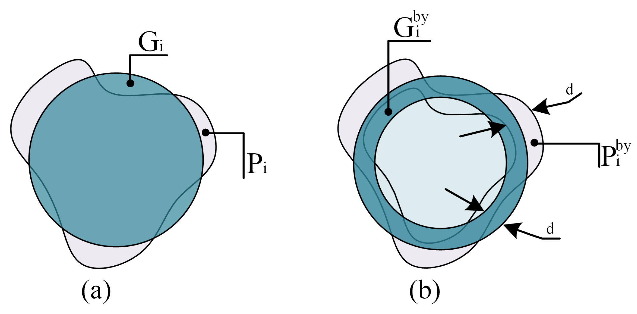
2.4. Boundary-Aware Weighted Loss

For the final classification task of mask prediction, we combine the binary cross-entropy (BCE) loss model with the Dice loss model based on boundary area design to handle class imbalance and instability. For i samples, $y_i$ and ${\tilde{y}}_i$ denote the true ground labeling probability and the predicted probability of sample i. The definition of BCE Loss ($L_{BCE}$) is as follows:

$$L_{BCE}=-\frac{1}{N}\sum _{i=1}^N(y_i\times log\left({\tilde{y}}_i\right)+(1-y_i)\times log(1-{\tilde{y}}_i))$$

(1)

Inspired by the Dice loss function and recognizing the high demand for boundary segmentation in agricultural parcel extraction tasks, we have devised a Dice loss function based on the boundary area, termed Boundary Dice Loss ($L_{BYDice}$). The Dice loss function quantifies the similarity between predicted and ground truth regions by evaluating the ratio of their intersection to their union, thereby assessing segmentation accuracy. This approach guides the model to better comprehend the characteristics of boundary areas in agricultural parcels, enhancing the precision of edge segmentation. As depicted in Figure 6a, the light purple area denotes the predicted region $P_i$ for class i, while the deep blue area represents the true region $G_i$. To avoid situations where both the numerator and denominator are 0, we introduce a constant ∈.

$$L_{BYDice}=\frac{1}{N}\sum _{i=0}^{N-1}(1-\frac{2|P_i^{by}\cap G_i^{by}|+\in }{|P_i^{by}|+|G_i^{by}|+\in })$$

(2)

Finally, by introducing weight parameters ${\omega }_1$ and ${\omega }_2$, after multiple tests, it is confirmed that ${\omega }_1={\omega }_2=0.5$ yields the best results. The final loss algorithm calculation formula is as follows:

$$Loss=L_{BYDcie}\times {\omega }_1+L_{BCE}\times {\omega }_2$$

(3)

3. Experiments

3.1. Dataset

The experimental data utilized in this study are detailed in Figure 7. Figure 7a presents the Sentinel-2 satellite imagery of the Denmark region, while Figure 7b displays the GaoFen-2 satellite imagery of the Shandong region in China. The Denmark dataset encompasses a vast area with densely distributed and variously sized agricultural parcels, whereas the Shandong dataset covers a smaller area with more regularly shaped agricultural parcels. The boundaries in both datasets are clearly defined. The ground truth data for the Denmark dataset were sourced from the European Union’s Land Parcel Identification System (LPIS), while the ground truth for the Shandong dataset was manually annotated. Detailed information about the datasets is provided in

Table 1. Detailed information about the dataset.

Areas	Satellites	Dates	Resolution (m)	Size (pixels)	Area (km2)
Denmark	Sentinel-2	8 May 2016	10	10,982 × 20,978	20,900
Shandong	Gaofen-2	20 December 2021	1	10,661 × 8769	91.70

. We divided the datasets into training, validation, and testing sets as delineated in Figure 7, with corresponding sample images shown in the insets. To preserve edge information and mitigate overfitting, the original images were cropped with a 30% overlap. For the Denmark dataset, we obtained 4872 unaugmented training slices measuring 256 × 256, 1382 testing slices, and 967 validation slices. For the Shandong dataset, we acquired 2049 unaugmented training slices measuring 256 × 256, 567 testing slices, and 407 validation slices. To enhance the generalizability of the model, we additionally applied data augmentation techniques to the training sets of both datasets, including horizontal flipping, vertical flipping, and 90-degree clockwise rotation.

3.2. Implementation Details

The DSTBA-Net was constructed within the PyTorch deep learning framework and trained using an NVIDIA RTX 3090 (24G) GPU. To achieve rapid convergence of the network, we utilized the Stochastic Gradient Descent (SGD) optimizer with a momentum of 0.9 and a weight decay of $1\times e^{-4}$ to optimize the backpropagation process of DSTBA-Net. This approach involved training on the Denmark dataset for 100 epochs and on the Shandong dataset for 70 epochs, ultimately reaching a state of convergence.

3.3. Evaluation Metrics

To quantitatively measure the performance of DSTBA-Net, we employed several commonly used evaluation metrics in semantic segmentation: Overall Accuracy ($OA$), Recall (R), F1-score ($F1$), and Intersection over Union ($IoU$). Specifically, these metrics are defined by the following formulas:

$$OA=\frac{TP+TN}{TP+TN+FP+FN}$$

(4)

$$P=\frac{TP}{TP+FP}$$

(5)

$$R=\frac{TP}{TP+FN}$$

(6)

$$F1=2\times \frac{P\times R}{P+R}$$

(7)

where $TP$, $TN$, $FP$, and $FN$ represent true positives, true negatives, false positives, and false negatives, respectively.

$OA$ is the percentage of correctly predicted samples out of the total samples. Generally, the higher the accuracy, the better the segmentation effect. P is the probability that a sample predicted as positive is actually positive. R indicates the probability that a positive sample is predicted as positive. The $F1$ considers both P and R, aiming to maximize and balance them simultaneously. $IoU$ determines the extent to which target features are captured, maximizing the intersection between predicted labels and annotations to ascertain model accuracy. It is calculated as follows:

$$I\mathrm{o}U=\frac{|P_p\cap P_{\mathrm{t}}|}{|P_p\cup P_{\mathrm{t}}|}$$

(8)

where $P_p$ represents the set of pixels predicted as agricultural parcels, and $P_t$ represents the set of pixels of actual parcels. $|.|$ denotes the function to calculate the number of pixels in a set.

In addition to the above metrics, to verify the effectiveness of this method in boundary shape learning, two boundary metrics were used for quantitative evaluation: Hausdorff distance ($HD$) and structural similarity ($SSIM$). As a measure of shape similarity, $HD$ is more sensitive to the boundaries of segmentation. It is defined as follows.

$HD$ between two sets, X and Y, is the maximum distance of a point set to the nearest point in the other set. In image segmentation tasks, it is used to measure the shape similarity between prediction results and actual labels. Specifically,

$$\begin{array}{cc}\hfill d_H(X,Y)& =max\{d_{XY},d_{YX}\}=max\{\underset{x\in X}{max}\underset{y\in Y}{min}(x,y),\underset{y\in Y}{max}\underset{x\in X}{min}(x,y)\}\hfill \end{array}$$

(9)

where X and Y are the ground truth and predicted maps, respectively. $d_H(X,Y)$ is the distance between points x and y. To mitigate the impact of outliers, $HD$ is multiplied by $95\%$ to obtain the final metric ($95\%HD$). The smaller the distance, the closer the predicted shape is to the actual label.

The Structural Similarity Index ($SSIM$) considers the brightness, contrast, and structure of images, commonly used to measure the similarity between two images. It is defined as

$$\begin{array}{cc}\hfill S(X,Y)& =F(l(X,Y),c(X,Y),s(X,Y))=\frac{(2{\mu }_x{\mu }_y+C_1)(2{\sigma }_{xy}+C_2)}{({\mu }_x^2+{\mu }_y^2+C_1)({\sigma }_x^2+{\sigma }_y^2+C_2)}\hfill \end{array}$$

(10)

where $\mu$, $\sigma$, and ${\sigma }_{xy}$ represent the mean, variance, and covariance, respectively. $C_1$ and $C_2$ are constants to avoid division by zero, typically set to 6.50 and 58.52. $SSIM$ ranges within (−1, 1), with a value of 1 indicating identical images.

4. Results

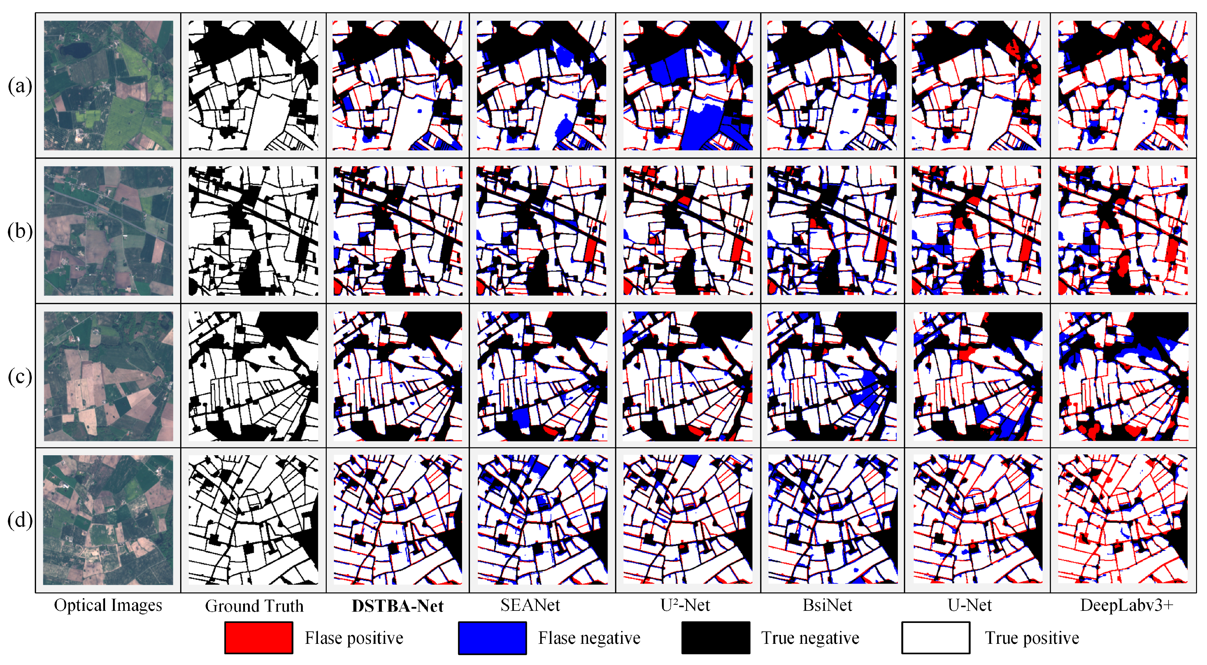
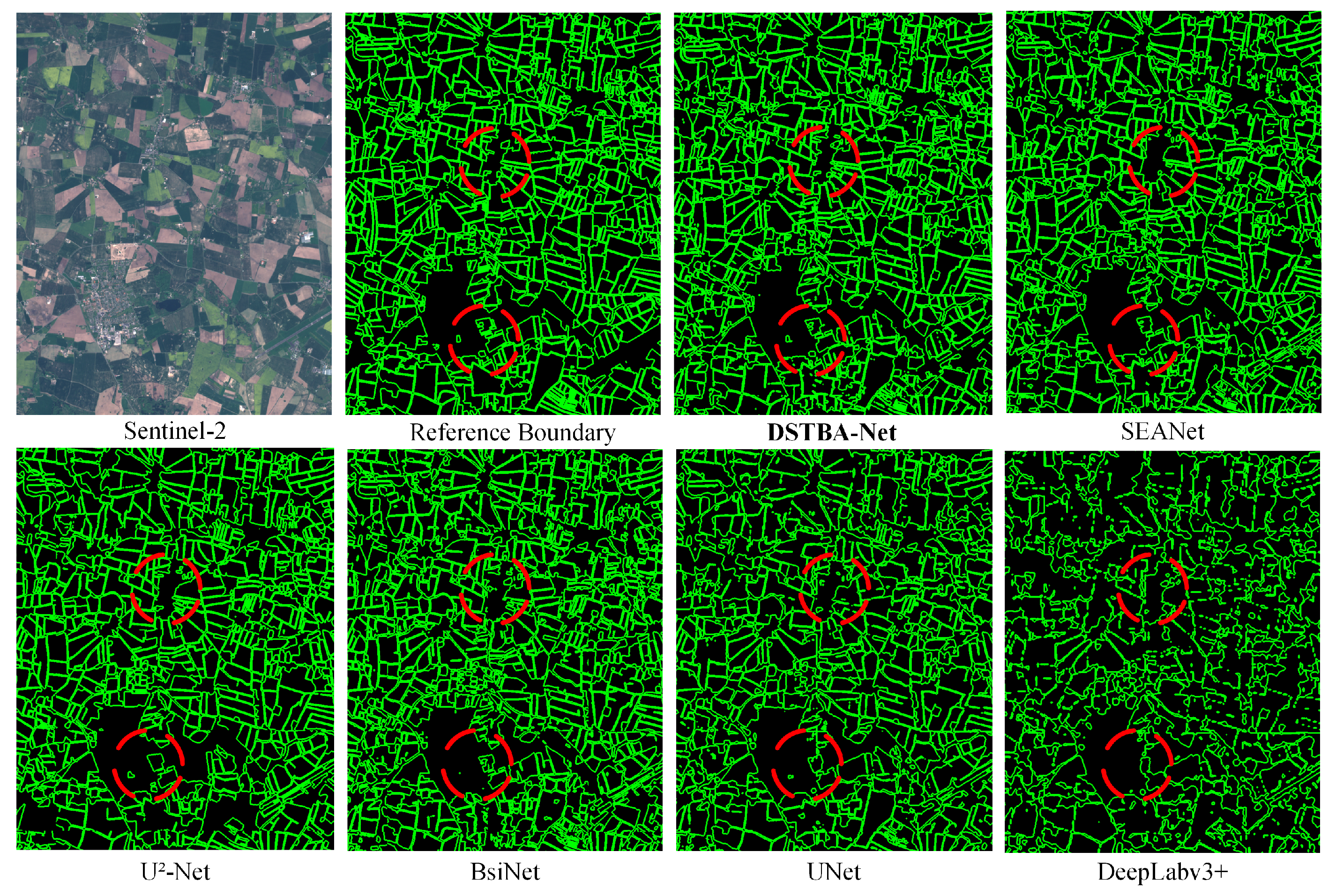
4.1. Experiment Using the Denmark Sentinel-2 Image

Figure 8 illustrates the experimental results of our proposed method on the Denmark dataset. It can be observed that our method achieves consistent boundary delineation for agricultural parcels of varying sizes and shapes. This demonstrates the effectiveness of our model on medium-resolution remote sensing imagery. In addition, in Figure 9, we visualize the error of extraction results. Red and blue indicate the number of pixels incorrectly predicted as farmland and non-farmland, respectively, while black and white represent the number of pixels correctly predicted as non-farmland and farmland. We compare these visualizations with two classical semantic segmentation models and three recent agricultural parcels extraction models. Four representative images from the test set are selected for display, as shown in Figure 9a–d. Comparative experiments are conducted using SEANet, U²-Net [59], BsiNet [60], U-Net, DeepLabv3+ [61], and DSTBA-Net. Here are brief descriptions of the five comparative models. First, the classical semantic segmentation models U-Net and Deeplabv3+. U-Net combines skip connections in the decoder part to better capture multi-scale information and reduce information loss. Deeplabv3+ employs techniques such as atrous convolution to enlarge the receptive field, enhancing segmentation accuracy and efficiency. U²-Net, designed for saliency object detection tasks, achieves superior binary classification performance by combining and merging the outputs of multiple U-Net networks. Lastly, the advanced multi-task segmentation networks SEANet and BsiNet integrate mask prediction, edge prediction, and distance map estimation. By extracting rich edge features at multiple levels, they significantly improve the accuracy of agricultural parcel extraction. The second column in Figure 9 represents the ground truth, followed by the depiction of errors in agricultural plot extraction from different models. All models are trained using the recommended loss functions and formulations from the existing literature, and all experiments are conducted under the same conditions as DSTBA-Net.

In general, both classic methods, U-Net and Deeplabv3+, exhibit blurred boundaries and considerable adhesion between agricultural parcels, making it challenging to obtain distinct and independent delineations of these parcels. Conversely, the latest agricultural plot extraction models, namely SEANet, U²-Net, and BsiNet, offer clearer and more pronounced boundaries compared to traditional approaches. However, they still suffer from varying degrees of misclassification and omission within the parcels.

Specifically, in Figure 9, the first two rows depict close-ups of extraction results in complex backgrounds, while the third row showcases results from relatively dense and regular areas. The fourth row illustrates results from contiguous regions. Due to interference from factors such as grassland and bare soil, the other five test models exhibit more instances of plot omission and misclassification in (a) and (b). In contrast, our network benefits from a robust feature encoder, resulting in significantly lower errors compared to other methods. For densely packed parcels in (c), our network accurately delineates plot contours. Similarly, DSTBA-Net performs best in extracting contiguous agricultural parcels, yielding optimal plot extraction and boundary delineation in (d). Consequently, our approach achieves comprehensive extraction on the medium-resolution Denmark dataset.

To visualize the boundary extraction performance of the models more intuitively, the extracted agricultural parcel boundaries were refined using morphological methods in this study. Figure 10 shows the boundary extraction results of several models in a test area in Denmark. We marked the extraction results of different models for the same detail with a red dashed line, and the comparison clearly shows that our model achieves more complete and accurate results.

The quantitative evaluation results of this study are presented in

Table 2. Quantitative evaluation on the denmark dataset.

Method	Common Metrics					Boundary Metrics
	OA (%)	P (%)	R (%)	F 1 (%)	IoU (%)	95% HD	SSIM (%)
DSTBA-Net	93.00	87.13	86.03	85.90	78.13	97.73	81.26
SEANet	92.20	86.84	85.28	85.50	77.04	93.86	79.34
U2-Net	92.14	83.70	86.19	84.36	76.06	125.56	79.57
BsiNet	91.03	85.00	81.91	82.92	73.77	104.84	76.53
U-Net	86.68	73.87	86.53	79.25	68.87	98.84	71.41
Deeplabv3+	85.75	73.38	86.94	78.83	68.37	104.35	69.13

Bold indicates the best result for the metric, and underline indicates the second-best result.

. Five commonly used semantic segmentation evaluation metrics and two boundary shape metrics were selected for calculation. The best results are highlighted in bold, while the second-best results are underlined.

Table 2 demonstrates the outstanding performance of DSTBA-Net across all evaluation metrics, with DSTBA-Net achieving a P value of 87.13% and R value of 86.03%. DSTBA-Net outperforms in $OA$, P, $F1$, and $I\mathrm{o}U$, reaching 93.00%, 87.13%, 85.90%, and 78.13%, respectively. This indicates our method’s ability to balance between P value and R value, maximizing identification while minimizing misclassifications and omissions of agricultural parcels. Additionally, our proposed method achieves the second lowest $95\%HD$ score and the highest $SSIM$ score, at 97.73% and 81.26%, respectively. Among the comparative models, SEANet exhibits the best overall performance, with $OA$, P, $F1$, and $I\mathrm{o}U$ being the second-best among all methods. Furthermore, it obtains the lowest $95\%HD$ score, suggesting significant advantages in boundary shape learning. However, its $SSIM$ score is lower than ours, indicating room for improvement in overall image similarity. Overall, our network remains advanced in learning agricultural plot boundaries. Particularly noteworthy is the substantial misclassification observed in the extraction results of Deeplabv3+, which biases the overall performance to display a high R value. Thus, a high value in this metric alone does not necessarily represent the ideal predictive performance of the method.

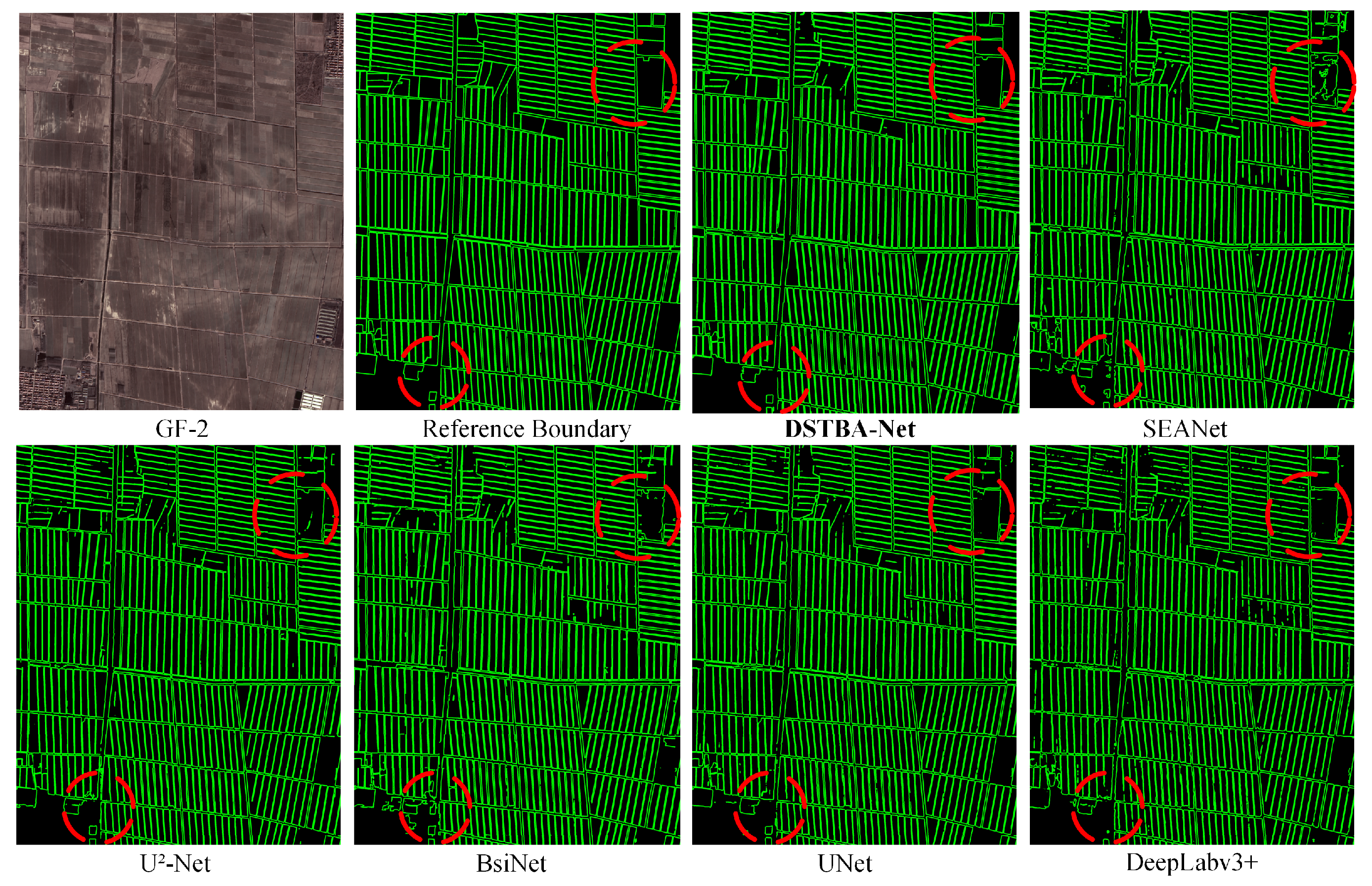
4.2. Experiment Using the Shandong GF-2 Image

To further assess the generalization performance of DSTBA-Net in extracting agricultural parcels across different datasets, experiments were conducted on a self-constructed Shandong dataset in this study. Figure 11 presents the extraction results of our method on the Shandong dataset, demonstrating high consistency with ground truth values across images with both dense and regular layouts. Similarly, error visualizations of the Shandong dataset test results are shown in Figure 12.

In Figure 12, the first and fourth rows depict close-ups of extracted agricultural parcels in regular layouts, while the second and third rows display results from dense layouts. It can be observed from the images that our method achieves the lowest segmentation errors, corresponding to minimal errors and omissions, particularly in cases with unclear boundaries. DSTBA-Net outperforms other methods in boundary extraction and effectively preserves the original shapes of agricultural parcels. This approach achieves comprehensive extraction on the high-resolution Shandong dataset. Additionally, in a test area of Shandong, we compared the extracted agricultural plot results from several models, as shown in Figure 13. Specifically, we employed sliding window and dilation prediction methods to perform predictions on the entire image, as illustrated in Figure 14.

Table 3. Quantitative evaluation on the Shandong dataset.

Method	Common Metrics					Boundary Metrics
	OA (%)	P (%)	R (%)	F 1 (%)	IoU (%)	95% HD	SSIM (%)
DSTBA-Net	95.05	96.51	96.47	96.46	93.24	54.57	84.29
SEANet	93.45	96.57	93.42	94.76	91.82	70.68	80.86
U2-Net	92.34	95.47	91.97	93.59	88.51	56.57	84.15
BsiNet	94.49	95.20	94.74	94.73	91.48	60.92	83.59
U-Net	91.19	89.67	96.73	92.86	87.52	80.00	81.95
Deeplabv3+	93.37	95.08	95.37	95.11	90.89	49.04	80.78

Bold indicates the best result for the metric, and underline indicates the second-best result.

presents the quantitative evaluation results for the Shandong dataset. Specifically, DSTBA-Net achieves the highest $OA$, $F1$, and $I\mathrm{o}U$, at 95.05%, 96.46%, and 93.24%, respectively. This further validates that our method can ensure the integrity of extraction results even in the presence of background features such as bare soil and built-$OA$up areas. As shown in the second and third rows of Figure 12, irregular parcels are common in the Shandong dataset, characterized by thin boundaries and challenging spectral information differentiation. Consequently, our P value and R value are slightly lower than other methods, at 96.51% and 96.47%, respectively. On the Shandong dataset, DSTBA-Net obtains the second lowest $95\%HD$ score and the highest $SSIM$ score, at 54.57% and 84.29%, respectively. Although DeepLabv3+ achieves the lowest $95\%HD$ score, its notable omission phenomena result in inferior performance in capturing the shape details of farmland, hence the lower $SSIM$. The metrics in Table 3 corroborate the superiority of our proposed method in shape learning, whereby DSTBA-Net effectively optimizes the boundaries of agricultural parcels, facilitating fine-grained segmentation at the plot level.

4.3. Ablation Experiments of DSTBA-Net

In this study, we conducted a whole-frame ablation experiment on the Danish dataset to validate the effectiveness of the proposed method and evaluate its performance. In addition, we have selected example images from two datasets to visualize the feature maps during the coding and decoding processes to further illustrate the usefulness of the proposed module.

The design of ablation experiments for the DSTBA-Net network framework is presented in

Table 4. Ablation No explanation needed. experiment setup of DSTBA-Net.

Model Name	Modules
	Baseline	Residual Block	BFG	GGFM
(a)	✓
(b)	✓	✓
(c)	✓	✓	✓
(d)	✓	✓		✓
(e)	✓	✓	✓	✓

, with detailed experimental results provided in

Table 5. Quantitative evaluation of ablation experiments.

Model	Common Metrics					Boundary Metrics
	OA (%)	P (%)	R (%)	F 1 (%)	IoU (%)	95% HD	SSIM (%)
(a)	86.68	73.87	86.53	79.25	68.87	98.84	71.41
(b)	87.76	75.91	87.23	81.19	71.27	101.54	72.04
(c)	90.16	83.42	83.13	82.47	74.11	99.98	76.32
(d)	91.60	84.51	83.98	83.37	75.02	104.59	77.55
(e)	93.00	87.13	86.03	85.90	78.13	97.73	81.26

Bold indicates the best result for the metric.

. The optimal results are highlighted in bold. Specifically, (a) denotes the baseline, which is the basic fully convolutional U-Net framework, and (b) represents the addition of the proposed Residual Block to (a) as an auxiliary encoder, which captures finer-grained features and enhances feature learning capabilities. Compared to (a), (b) achieves an overall accuracy (OA) improvement of 1.08% and an $I\mathrm{o}U$ increase of 2.40%, with this scheme obtaining the best R value. (c) adds Boundary Feature Guidance (BFG) to (b), effectively integrating boundary data features into the model, allowing the model to explicitly focus on boundary features and enhancing boundary information capture. Compared to (b), which does not include boundary features, (c) achieves an OA improvement of 2.40% and an $I\mathrm{o}U$ increase of 2.84%. (d) introduces the Global Feature Fusion Module (GFFM) to (b), leveraging the powerful encoding capabilities of the Transformer to establish long-distance dependencies between detailed and global features, and fuse feature maps generated from image data. Results show that adding GFFM increases the OA by 3.84% and the $I\mathrm{o}U$ by 3.75% compared to (b). (e) combines BFG, completing the acquisition of detailed features from image and boundary data and integrating them with global features, forming the complete DSTBA-Net. (e) achieved the best results in most metrics. Compared to (c), its OA and $I\mathrm{o}U$ increased by 2.84% and 4.02%, respectively, and compared to (d), its OA and $I\mathrm{o}U$ improved by 1.40% and 3.11%, respectively. These results further demonstrate the effectiveness of DSTBA-Net.

5. Discussion

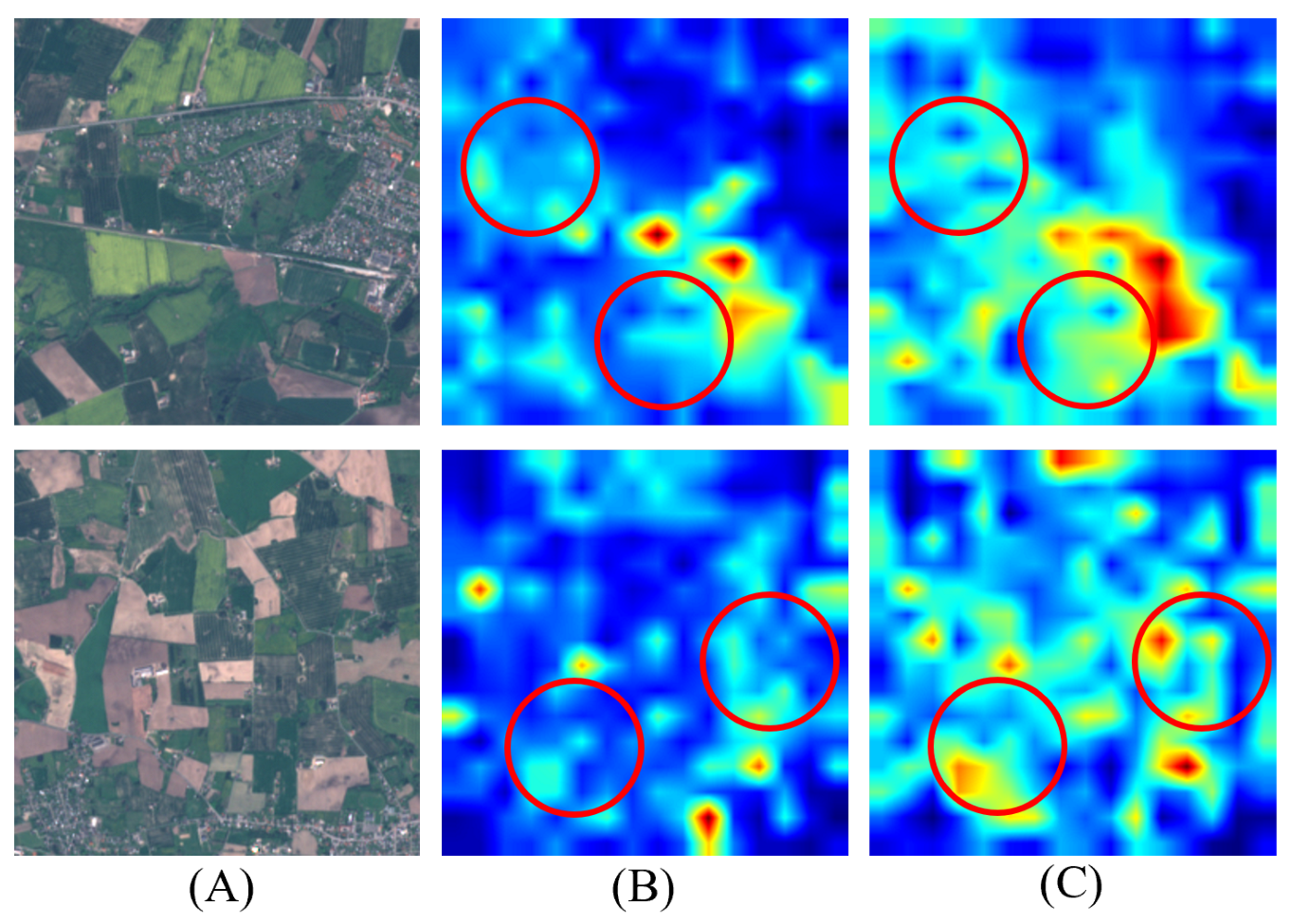
5.1. Module-Wise Feature Map Analysis

To further explore the impact of the proposed modules on feature extraction, we selected images from both datasets and used maximum activation value visualization to examine the changes in the feature maps with and without the addition of different modules.

Figure 15 shows the four-layer feature maps of the image slices from the Shandong dataset in the encoder, obtained by using ordinary convolution and residual convolution in our basic network, respectively. As can be seen from Figure 15, $\widehat{x^l}$ is more focused on the boundaries of the agricultural parcels than $x^l$. Although more low-level information is extracted as the model continues to encode, richer and more homogeneous semantic information is obtained using the Residual Block.

Figure 16 shows a comparison of the feature maps obtained with the basic network and after adding Boundary Feature Guidance (BFG). We have chosen two image slices from the Denmark dataset for this presentation. Panels (A), (B), and (C) denote the selected images, the feature maps before adding BFG, and the feature maps after adding BFG, respectively. As can be seen from Figure 16, (C) acquires richer low-level semantic information relative to (B). This indicates that BFG encourages the model to pay more attention to edge information in the image.

Figure 17 shows a comparison of the feature maps obtained in the decoder for the basic network and the model after adding the Global Feature Fusion Module (GFFM). An image slice from the Denmark dataset was selected for this presentation. Here, $y^l$ represents the feature map obtained from the basic network, $y^{\prime l}$ represents the feature map obtained by adding Feature Compensation Restoration (FCR), and $\widehat{y^l}$ represents the feature map obtained by adding GFFM.

As can be seen in Figure 17, $y^{\prime l}$ contains more complete edge semantic information and a more uniform distribution compared to $y^l$. $y^l$ exhibits excessively high intensity in some regions and lacks balanced information fusion, which is improved in $y^{\prime l}$. $\widehat{y^l}$, as the feature map after adding the Global Feature Fusion Module (GFFM), has richer and more complete semantic and location information compared to $y^l$. After the addition of GFFM, the model captures more long-range information during the upsampling process, which also aids in the final segmentation.

5.2. Analysis of Weight Coefficients

To further investigate the impact of weight coefficients in the proposed boundary-aware weighted loss algorithm, denoted as ${\omega }_1$ and ${\omega }_2$ (${\omega }_1+{\omega }_2=1$), we conducted additional experiments. The results in

Table 6. Influence of the coefficients in the loss function.

Coefficient (${\mathit{\omega }}_1$)	Common Metrics					Boundary Metrics
	OA (%)	P (%)	R (%)	F 1 (%)	IoU (%)	95% HD	SSIM (%)
0.3	91.70	85.55	84.41	84.18	75.91	114.86	78.68
0.4	92.24	86.19	84.84	84.55	76.36	107.37	79.24
0.5	93.00	87.13	86.03	85.90	78.13	97.73	81.26
0.6	92.63	86.15	85.76	85.15	77.13	105.42	80.09
0.7	91.81	85.60	84.11	84.07	75.93	110.40	78.71

Bold indicates the best result for the metric.

demonstrate that the model achieves optimal performance when ${\omega }_1={\omega }_2=0.5$. This suggests that under this coefficient setting, the model effectively balances boundary loss and other losses, resulting in optimal scores across all metrics. Particularly noteworthy is the significant improvement in P and R values, indicating better extraction accuracy and efficiency achieved by our method.

5.3. Discussion on Data Variability

This study selected datasets from Denmark and Shandong for experimentation. Due to differences in resolution, field shapes, and agricultural parcels between the datasets, using the same method for parcel extraction may yield different results. For instance, Shandong’s vegetation may be influenced by distinct climatic and soil characteristics, resulting in different vegetation features and growth patterns compared to Denmark. Therefore, when comparing and analyzing the results, it is essential to further consider these differences in growth stages and environmental factors. Further research is needed to address these variations comprehensively.

6. Conclusions

This study introduces DSTBA-Net, a method for agricultural parcel extraction that emphasizes boundary optimization and global information fusion. The network utilizes a dual-stream architecture to separately extract image and boundary features, which are then fused to incorporate captured fine-grained details and global contextual information, effectively addressing deficiencies in morphological feature optimization and segmentation completeness. We propose a boundary-aware weighted loss algorithm to appropriately balance the importance of parcel interiors and boundaries. To validate the performance of our network, experiments were conducted on datasets from Denmark and Shandong, China. Besides using standard semantic segmentation metrics, boundary evaluation metrics were also employed to quantitatively demonstrate the advantages of DSTBA-Net in boundary delineation. Experimental results on both datasets indicate that our proposed network surpasses state-of-the-art networks in the accuracy of agricultural parcel extraction. This research also includes ablation studies, which verify that the Dual-Stream Feature Extraction (DSFE) and the Global Feature Fusion Module (GFFM) significantly enhance network performance. Our method can effectively extract agricultural parcels from remote sensing images with different agricultural parcels and at various scales, providing a solution for addressing challenges in complex environments.

References

1. Kocur-Bera, K. Data compatibility between the Land and Building Cadaster (LBC) and the Land Parcel Identification System (LPIS) in the context of area-based payments: A case study in the Polish Region of Warmia and Mazury. Land Use Policy 2019, 80, 370–379. [Google Scholar] [CrossRef]
2. McCarty, J.; Neigh, C.; Carroll, M.; Wooten, M. Extracting smallholder cropped area in Tigray, Ethiopia with wall-to-wall sub-meter WorldView and moderate resolution Landsat 8 imagery. Remote Sens. Environ. 2017, 202, 142–151. [Google Scholar] [CrossRef]
3. Belgiu, M.; Csillik, O. Sentinel-2 cropland mapping using pixel-based and object-based time-weighted dynamic time warping analysis. Remote Sens. Environ. 2018, 204, 509–523. [Google Scholar] [CrossRef]
4. Sitokonstantinou, V.; Papoutsis, I.; Kontoes, C.; Lafarga Arnal, A.; Armesto Andres, A.P.; Garraza Zurbano, J.A. Scalable parcel-based crop identification scheme using Sentinel-2 data time-series for the monitoring of the common agricultural policy. Remote Sens. 2018, 10, 911. [Google Scholar] [CrossRef]
5. Dong, W.; Wu, T.; Luo, J.; Sun, Y.; Xia, L. Land parcel-based digital soil mapping of soil nutrient properties in an alluvial-diluvia plain agricultural area in China. Geoderma 2019, 340, 234–248. [Google Scholar] [CrossRef]
6. Wagner, M.P.; Oppelt, N. Extracting agricultural fields from remote sensing imagery using graph-based growing contours. Remote Sens. 2020, 12, 1205. [Google Scholar] [CrossRef]
7. Tang, Z.; Li, M.; Wang, X. Mapping tea plantations from VHR images using OBIA and convolutional neural networks. Remote Sens. 2020, 12, 2935. [Google Scholar] [CrossRef]
8. Graesser, J.; Ramankutty, N. Detection of cropland field parcels from Landsat imagery. Remote Sens. Environ. 2017, 201, 165–180. [Google Scholar] [CrossRef]
9. Xiong, J.; Thenkabail, P.S.; Gumma, M.K.; Teluguntla, P.; Poehnelt, J.; Congalton, R.G.; Yadav, K.; Thau, D. Automated cropland mapping of continental Africa using Google Earth Engine cloud computing. ISPRS J. Photogramm. Remote Sens. 2017, 126, 225–244. [Google Scholar] [CrossRef]
10. Waldner, F.; Canto, G.S.; Defourny, P. Automated annual cropland mapping using knowledge-based temporal features. ISPRS J. Photogramm. Remote Sens. 2015, 110, 1–13. [Google Scholar] [CrossRef]
11. Jong, M.; Guan, K.; Wang, S.; Huang, Y.; Peng, B. Improving field boundary delineation in ResUNets via adversarial deep learning. Int. J. Appl. Earth Obs. Geoinf. 2022, 112, 102877. [Google Scholar] [CrossRef]
12. Cai, Z.; Hu, Q.; Zhang, X.; Yang, J.; Wei, H.; He, Z.; Song, Q.; Wang, C.; Yin, G.; Xu, B. An adaptive image segmentation method with automatic selection of optimal scale for extracting cropland parcels in smallholder farming systems. Remote Sens. 2022, 14, 3067. [Google Scholar] [CrossRef]
13. Hossain, M.D.; Chen, D. Segmentation for Object-Based Image Analysis (OBIA): A review of algorithms and challenges from remote sensing perspective. ISPRS J. Photogramm. Remote Sens. 2019, 150, 115–134. [Google Scholar] [CrossRef]
14. Rydberg, A.; Borgefors, G. Integrated method for boundary delineation of agricultural fields in multispectral satellite images. IEEE Trans. Geosci. Remote Sens. 2001, 39, 2514–2520. [Google Scholar] [CrossRef]
15. Robb, C.; Hardy, A.; Doonan, J.H.; Brook, J. Semi-automated field plot segmentation from UAS imagery for experimental agriculture. Front. Plant Sci. 2020, 11, 591886. [Google Scholar] [CrossRef]
16. Hong, R.; Park, J.; Jang, S.; Shin, H.; Kim, H.; Song, I. Development of a parcel-level land boundary extraction algorithm for aerial imagery of regularly arranged agricultural areas. Remote Sens. 2021, 13, 1167. [Google Scholar] [CrossRef]
17. Suzuki, S. Topological structural analysis of digitized binary images by border following. Comput. Vision Graph. Image Process. 1985, 30, 32–46. [Google Scholar] [CrossRef]
18. Canny, J. A computational approach to edge detection. IEEE Trans. Pattern Anal. Mach. Intell. 1986, 6, 679–698. [Google Scholar] [CrossRef]
19. Kecman, V. Support vector machines—An introduction. In Support Vector Machines: Theory and Applications; Springer: Berlin/Heidelberg, Germany, 2005; pp. 1–47. [Google Scholar]
20. Li, D.; Zhang, G.; Wu, Z.; Yi, L. An edge embedded marker-based watershed algorithm for high spatial resolution remote sensing image segmentation. IEEE Trans. Image Process. 2010, 19, 2781–2787. [Google Scholar]
21. Chen, B.; Qiu, F.; Wu, B.; Du, H. Image segmentation based on constrained spectral variance difference and edge penalty. Remote Sens. 2015, 7, 5980–6004. [Google Scholar] [CrossRef]
22. Benz, U.C.; Hofmann, P.; Willhauck, G.; Lingenfelder, I.; Heynen, M. Multi-resolution, object-oriented fuzzy analysis of remote sensing data for GIS-ready information. ISPRS J. Photogramm. Remote Sens. 2004, 58, 239–258. [Google Scholar] [CrossRef]
23. Wassie, Y.; Koeva, M.; Bennett, R.; Lemmen, C. A procedure for semi-automated cadastral boundary feature extraction from high-resolution satellite imagery. J. Spat. Sci. 2018, 63, 75–92. [Google Scholar] [CrossRef]
24. Torre, M.; Radeva, P. Agricultural-field extraction on aerial images by region competition algorithm. In Proceedings of the Proceedings 15th International Conference on Pattern Recognition, Barcelona, Spain, 3–7 September 2000; ICPR-2000. IEEE: Piscataway, NJ, USA, 2000; Volume 1, pp. 313–316. [Google Scholar]
25. Tetteh, G.O.; Gocht, A.; Schwieder, M.; Erasmi, S.; Conrad, C. Unsupervised parameterization for optimal segmentation of agricultural parcels from satellite images in different agricultural landscapes. Remote Sens. 2020, 12, 3096. [Google Scholar] [CrossRef]
26. Garcia-Pedrero, A.; Gonzalo-Martin, C.; Lillo-Saavedra, M. A machine learning approach for agricultural parcel delineation through agglomerative segmentation. Int. J. Remote Sens. 2017, 38, 1809–1819. [Google Scholar] [CrossRef]
27. Tian, Y.; Yang, C.; Huang, W.; Tang, J.; Li, X.; Zhang, Q. Machine learning-based crop recognition from aerial remote sensing imagery. Front. Earth Sci. 2021, 15, 54–69. [Google Scholar] [CrossRef]
28. Guo, H.; Shi, Q.; Marinoni, A.; Du, B.; Zhang, L. Deep building footprint update network: A semi-supervised method for updating existing building footprint from bi-temporal remote sensing images. Remote Sens. Environ. 2021, 264, 112589. [Google Scholar] [CrossRef]
29. Shi, Q.; Liu, M.; Li, S.; Liu, X.; Wang, F.; Zhang, L. A deeply supervised attention metric-based network and an open aerial image dataset for remote sensing change detection. IEEE Trans. Geosci. Remote Sens. 2021, 60, 1–16. [Google Scholar] [CrossRef]
30. Liu, S.; Shi, Q.; Zhang, L. Few-shot hyperspectral image classification with unknown classes using multitask deep learning. IEEE Trans. Geosci. Remote Sens. 2020, 59, 5085–5102. [Google Scholar] [CrossRef]
31. Shi, Q.; Tang, X.; Yang, T.; Liu, R.; Zhang, L. Hyperspectral image denoising using a 3-D attention denoising network. IEEE Trans. Geosci. Remote Sens. 2021, 59, 10348–10363. [Google Scholar] [CrossRef]
32. Zhang, C.; Sargent, I.; Pan, X.; Li, H.; Gardiner, A.; Hare, J.; Atkinson, P.M. Joint Deep Learning for land cover and land use classification. Remote Sens. Environ. 2019, 221, 173–187. [Google Scholar] [CrossRef]
33. He, D.; Shi, Q.; Liu, X.; Zhong, Y.; Zhang, X. Deep subpixel mapping based on semantic information modulated network for urban land use mapping. IEEE Trans. Geosci. Remote Sens. 2021, 59, 10628–10646. [Google Scholar] [CrossRef]
34. Zhang, D.; Pan, Y.; Zhang, J.; Hu, T.; Zhao, J.; Li, N.; Chen, Q. A generalized approach based on convolutional neural networks for large area cropland mapping at very high resolution. Remote Sens. Environ. 2020, 247, 111912. [Google Scholar] [CrossRef]
35. Persello, C.; Bruzzone, L. A novel protocol for accuracy assessment in classification of very high resolution images. IEEE Trans. Geosci. Remote Sens. 2009, 48, 1232–1244. [Google Scholar] [CrossRef]
36. Liu, Y.; Cheng, M.M.; Hu, X.; Wang, K.; Bai, X. Richer convolutional features for edge detection. In Proceedings of the IEEE Conference on Computer Vision and Pattern Recognition, Honolulu, HI, USA, 21–26 July 2017; pp. 3000–3009. [Google Scholar]
37. Garcia-Pedrero, A.; Lillo-Saavedra, M.; Rodriguez-Esparragon, D.; Gonzalo-Martin, C. Deep learning for automatic outlining agricultural parcels: Exploiting the land parcel identification system. IEEE Access 2019, 7, 158223–158236. [Google Scholar] [CrossRef]
38. Li, C.; Fu, L.; Zhu, Q.; Zhu, J.; Fang, Z.; Xie, Y.; Guo, Y.; Gong, Y. Attention enhanced u-net for building extraction from farmland based on google and worldview-2 remote sensing images. Remote Sens. 2021, 13, 4411. [Google Scholar] [CrossRef]
39. Xia, L.; Zhao, F.; Chen, J.; Yu, L.; Lu, M.; Yu, Q.; Liang, S.; Fan, L.; Sun, X.; Wu, S.; et al. A full resolution deep learning network for paddy rice mapping using Landsat data. ISPRS J. Photogramm. Remote Sens. 2022, 194, 91–107. [Google Scholar] [CrossRef]
40. Long, J.; Shelhamer, E.; Darrell, T. Fully convolutional networks for semantic segmentation. In Proceedings of the IEEE Conference on Computer Vision and Pattern Recognition, Boston, MA, USA, 7–12 June 2015; pp. 3431–3440. [Google Scholar]
41. Ronneberger, O.; Fischer, P.; Brox, T. U-net: Convolutional networks for biomedical image segmentation. In Proceedings of the Medical Image Computing and Computer-Assisted Intervention—MICCAI 2015: 18th International Conference, Munich, Germany, 5–9 October 2015; proceedings, part III 18. Springer: Cham, Switzerland, 2015; pp. 234–241. [Google Scholar]
42. Guo, M.; Liu, H.; Xu, Y.; Huang, Y. Building extraction based on U-Net with an attention block and multiple losses. Remote Sens. 2020, 12, 1400. [Google Scholar] [CrossRef]
43. Xia, L.; Luo, J.; Sun, Y.; Yang, H. Deep extraction of cropland parcels from very high-resolution remotely sensed imagery. In Proceedings of the 2018 7th International Conference on Agro-Geoinformatics (Agro-Geoinformatics), Hangzhou, China, 6–9 August 2018; IEEE: Piscataway, NJ, USA, 2018; pp. 1–5. [Google Scholar]
44. Potlapally, A.; Chowdary, P.S.R.; Shekhar, S.R.; Mishra, N.; Madhuri, C.S.V.D.; Prasad, A. Instance segmentation in remote sensing imagery using deep convolutional neural networks. In Proceedings of the 2019 International Conference on Contemporary Computing and Informatics (IC3I), Singapore, 12–14 December 2019; IEEE: Piscataway, NJ, USA, 2019; pp. 117–120. [Google Scholar]
45. Waldner, F.; Diakogiannis, F.I. Deep learning on edge: Extracting field boundaries from satellite images with a convolutional neural network. Remote Sens. Environ. 2020, 245, 111741. [Google Scholar] [CrossRef]
46. Li, M.; Long, J.; Stein, A.; Wang, X. Using a semantic edge-aware multi-task neural network to delineate agricultural parcels from remote sensing images. ISPRS J. Photogramm. Remote Sens. 2023, 200, 24–40. [Google Scholar] [CrossRef]
47. Vaswani, A.; Shazeer, N.; Parmar, N.; Uszkoreit, J.; Jones, L.; Gomez, A.N.; Kaiser, L.; Polosukhin, I. Attention Is All You Need.(Nips), 2017. arXiv 2017, arXiv:1706.03762. [Google Scholar]
48. Aleissaee, A.A.; Kumar, A.; Anwer, R.M.; Khan, S.; Cholakkal, H.; Xia, G.S.; Khan, F.S. Transformers in remote sensing: A survey. Remote Sens. 2023, 15, 1860. [Google Scholar] [CrossRef]
49. Zheng, S.; Lu, J.; Zhao, H.; Zhu, X.; Luo, Z.; Wang, Y.; Fu, Y.; Feng, J.; Xiang, T.; Torr, P.H.; et al. Rethinking semantic segmentation from a sequence-to-sequence perspective with transformers. In Proceedings of the IEEE/CVF Conference on Computer Vision and Pattern Recognition, Nashville, TN, USA, 20–25 June 2021; pp. 6881–6890. [Google Scholar]
50. Wang, L.; Fang, S.; Meng, X.; Li, R. Building extraction with vision transformer. IEEE Trans. Geosci. Remote Sens. 2022, 60, 1–11. [Google Scholar] [CrossRef]
51. Chen, K.; Zou, Z.; Shi, Z. Building extraction from remote sensing images with sparse token transformers. Remote Sens. 2021, 13, 4441. [Google Scholar] [CrossRef]
52. Xiao, X.; Guo, W.; Chen, R.; Hui, Y.; Wang, J.; Zhao, H. A swin transformer-based encoding booster integrated in u-shaped network for building extraction. Remote Sens. 2022, 14, 2611. [Google Scholar] [CrossRef]
53. Wang, H.; Chen, X.; Zhang, T.; Xu, Z.; Li, J. CCTNet: Coupled CNN and transformer network for crop segmentation of remote sensing images. Remote Sens. 2022, 14, 1956. [Google Scholar] [CrossRef]
54. Xia, L.; Mi, S.; Zhang, J.; Luo, J.; Shen, Z.; Cheng, Y. Dual-stream feature extraction network based on CNN and transformer for building extraction. Remote Sens. 2023, 15, 2689. [Google Scholar] [CrossRef]
55. Ding, L.; Lin, D.; Lin, S.; Zhang, J.; Cui, X.; Wang, Y.; Tang, H.; Bruzzone, L. Looking outside the window: Wide-context transformer for the semantic segmentation of high-resolution remote sensing images. IEEE Trans. Geosci. Remote Sens. 2022, 60, 1–13. [Google Scholar] [CrossRef]
56. Gao, L.; Liu, H.; Yang, M.; Chen, L.; Wan, Y.; Xiao, Z.; Qian, Y. STransFuse: Fusing swin transformer and convolutional neural network for remote sensing image semantic segmentation. IEEE J. Sel. Top. Appl. Earth Obs. Remote Sens. 2021, 14, 10990–11003. [Google Scholar] [CrossRef]
57. Wang, Y.; Zhang, W.; Chen, W.; Chen, C. BSDSNet: Dual-Stream Feature Extraction Network Based on Segment Anything Model for Synthetic Aperture Radar Land Cover Classification. Remote Sens. 2024, 16, 1150. [Google Scholar] [CrossRef]
58. He, K.; Zhang, X.; Ren, S.; Sun, J. Deep residual learning for image recognition. In Proceedings of the IEEE Conference on Computer Vision and Pattern Recognition, Las Vegas, NV, USA, 27–30 June 2016; pp. 770–778. [Google Scholar]
59. Qin, X.; Zhang, Z.; Huang, C.; Dehghan, M.; Zaiane, O.R.; Jagersand, M. U2-Net: Going deeper with nested U-structure for salient object detection. Pattern Recognit. 2020, 106, 107404. [Google Scholar] [CrossRef]
60. Long, J.; Li, M.; Wang, X.; Stein, A. Delineation of agricultural fields using multi-task BsiNet from high-resolution satellite images. Int. J. Appl. Earth Obs. Geoinf. 2022, 112, 102871. [Google Scholar] [CrossRef]
61. Chen, L.C.; Zhu, Y.; Papandreou, G.; Schroff, F.; Adam, H. Encoder-decoder with atrous separable convolution for semantic image segmentation. In Proceedings of the European Conference on Computer Vision (ECCV), Munich, Germany, 8–14 September 2018; pp. 801–818. [Google Scholar]
Figure 1. Schematic of the proposed segmentation framework.
Remotesensing 16 02637 g001
Figure 2. Detailed process of the proposed network. x l ( l [ 1 , 2 , 3 , 4 ] ) represents the feature map obtained by the encoder. y l ( l [ 1 , 2 , 3 ] ) represents the feature map obtained by the decoder.
Remotesensing 16 02637 g002
Figure 3. Dual-stream feature extraction.
Remotesensing 16 02637 g003
Figure 4. Specific structure of the Convolution Block and Residual Block.
Remotesensing 16 02637 g004
Figure 5. The specific structure diagram of the Global Feature Fusion Module (GFFM).
Remotesensing 16 02637 g005
Figure 6. Schematic diagram of the Dice loss function based on boundary area. (a) The prediction results and ground truth of the i-th category. (b) The prediction result of the i-th class and the edge area of the ground truth; d is the width of the edge area.
Remotesensing 16 02637 g006
Figure 7. Overview of the dataset.
Remotesensing 16 02637 g007
Figure 8. Extracted agricultural parcels by DSTBA-Net on the Denmark (DK) Sentinel-2 image.
Remotesensing 16 02637 g008
Figure 9. Examples of agricultural parcels delineated by different methods on the Denmark dataset.(a,b) are image slices from areas with complex backgrounds; (c) is an image slice from a relatively regular area; (d) is an image slice from a contiguous distribution area.Examples of agricultural parcels delineated by different methods on the Denmark dataset.
Remotesensing 16 02637 g009
Figure 10. Examples of parcel boundaries extracted by different methods in a Denmark testing area.
Remotesensing 16 02637 g010
Figure 11. Extracted agricultural parcels by DSTBA-Net on the Shandong GF-2 image, China (CN).
Remotesensing 16 02637 g011
Figure 12. Examples of agricultural parcels delineated by different methods on the Shandong GF-2 image. (a,d) are image slices of agricultural parcels in regular layouts, while (b,c) are image slices of agricultural parcels in dense layouts.
Remotesensing 16 02637 g012
Figure 13. Examples of parcel boundaries extracted by different methods in a Shandong testing area.
Remotesensing 16 02637 g013
Figure 14. Prediction results for the entire Shandong dataset image. The white areas represent agricultural parcels, and the black areas represent non-agricultural parcels.
Remotesensing 16 02637 g014
Figure 15. Visualization of feature maps for Residual Block. x l and x l ^ , l [ 1 , 2 , 3 , 4 ] represent the Feature maps from regular convolution and provided Residual Blocks at each layer.
Remotesensing 16 02637 g015
Figure 16. Visualization of feature maps for BFG. (A) represents the selected image, (B) represents the feature maps before the addition of BFG, and (C) represents the feature maps after the addition of BFG.
Remotesensing 16 02637 g016
Figure 17. Visualization of feature maps for Residual Block. y l , y l and y l ^ , l [ 1 , 2 , 3 , 4 ] , respectively, denote the feature maps for each layer of the baseline network’s decoding part, after the inclusion of FCR, and after the inclusion of GFFM.
Remotesensing 16 02637 g017