Estimating Bermudagrass Aboveground Biomass Using Stereovision and Vegetation Coverage

Abstract

Accurate information about the amount of standing biomass is important in pasture management for monitoring forage growth patterns, minimizing the risk of overgrazing, and ensuring the necessary feed requirements of livestock. The morphological features of plants, like crop height and density, have been proven to be prominent predictors of crop yield. The objective of this study was to evaluate the effectiveness of stereovision-based crop height and vegetation coverage measurements in predicting the aboveground biomass yield of bermudagrass (Cynodon dactylon) in a pasture. Data were collected from 136 experimental plots within a 0.81 ha bermudagrass pasture using an RGB-depth camera mounted on a ground rover. The crop height was determined based on the disparity between images captured by two stereo cameras of the depth camera. The vegetation coverage was extracted from the RGB images using a machine learning algorithm by segmenting vegetative and non-vegetative pixels. After camera measurements, the plots were harvested and sub-sampled to measure the wet and dry biomass yields for each plot. The wet biomass yield prediction function based on crop height and vegetation coverage was generated using a linear regression analysis. The results indicated that the combination of crop height and vegetation coverage showed a promising correlation with aboveground wet biomass yield. However, the prediction function based only on the crop height showed less residuals at the extremes compared to the combined prediction function (crop height and vegetation coverage) and was thus declared the recommended approach (R² = 0.91; SeY= 1824 kg-wet/ha). The crop height-based prediction function was used to estimate the dry biomass yield using the mean dry matter fraction.

1. Introduction

Grasslands cover 70% of the agricultural lands and 26% of the world’s total land surface as of 2010 [1]. The majority of these grasslands are spread by human interventions to satisfy the need for increasing human and livestock populations. Bermudagrass is a warm season grass native to southeast Africa and is widely grown in the southeastern USA [2]. Hansen et al. [2] recommend beginning the grazing of bermudagrass when it becomes 15–20 cm tall, and until it reaches 8–10 cm of grazed height. If it grows more than 20 cm, it is suggested to be harvested as hay up to a uniform height of 8–10 cm. Depending on the growing season, plant growth is higher in the May to June period than the July to August period because of a greater amount of moisture availability [2]. These recommendations, however, change with the location and environmental conditions. Therefore, it becomes necessary to properly manage such grasslands and forages for optimal growth.

Visual estimation was traditionally practiced by growers and farmers to assess forage availability in grasslands [3]. These estimates accounted for factors like stage of maturity, color, leafiness, foreign material, and overall condition of the pasture. A well-experienced observer can make an acceptable prediction of the forage availability, but predictions might vary drastically among observers. Hence, some standardized methods for estimating forage availability were needed to eliminate the variability in biomass estimations. One such method is sampling and interpolation. In this method, a small area of 0.1 m² or a few such quadrants are harvested in the field and weighed to estimate the average biomass per unit harvested area. This average yield is then interpolated for the whole pasture. It is an effective way of measuring the available biomass, but is labor and time intensive, as well as a destructive method [4].

Several approaches have been used to predict aboveground biomass through indirect or non-destructive methods.

Table 1. Biomass estimation techniques/systems and their applicability in forage fields and grasslands.

Technique/System	Platform	Site Scale	Coefficient of Determination (R2) of Biomass Prediction Function
Spectral reflectance	Satellite (Landsat-8, Sentinal-2)	Large scale and farm scale	0.20–0.92 [5,6,7,8,9]
	Unmanned aerial vehicle (Hyperspectral camera)	Farm scale	0.42–0.92 [10,11]
LiDAR	Unmanned aerial vehicle and Unmanned ground vehicle	Farm scale and large scale	0.61–0.74 [12,13,14,15,16]
Structure from motion	Unmanned aerial vehicle	Farm scale	0.59–0.88 [17,18,19]
Ultrasound sensor	Unmanned ground vehicle	Farm scale	0.73–0.80 [20,21]
Meter stick, rising plate meter	Manual measurements	Farm scale	0.11–0.86 [22,23]

provides a summary of the coefficient of determinations (R²) of the biomass prediction functions developed for large scale and farm scale grasslands with space-borne, aerial-borne, and ground-borne systems and techniques.

Large-scale applications focus on the regional surveying and temporal analysis of crop features like yield, nitrogen content, and land cover change over the years on thousands of acres. On the other hand, farm scale applications facilitate the end users with the yield assessment for frequent management decisions. The results from Table 1 suggest that the coefficient of determination was better for the aerial and ground-based systems at their lower ranges of the R² values. However, some of the best coefficients of determination were also seen in the satellite-based systems as well (Table 1).

The long-term goal of this study was to develop forage yield prediction systems that are easy to use and are of practical utility for satisfying the farm scale needs of cattle and forage producers. For farm scale pasture management, the decisions related to the forage availability and stocking rate are made daily. The producer needs an update on which sections of the pasture can be used for cattle grazing and for how many days, before moving to the next section. Additionally, the decisions related to the harvesting of the forage for hay and silage are also scheduled based on the real-time conditions of the field produce. Any delay or unfavorable weather conditions might result in a significant decrement or loss of forage produce. Thus, it becomes critical to obtain the information about the forage availability on a daily basis.

In farm scale pasture productions, the management of the forage is taken care of by the producer and is sometimes supported by consultants for equipment or service requirements. The dependency on the consultancies for these resources might sometimes involve lesser flexibility and independence. The unavailability of the technician and the equipment in critical times might result in delayed management. So, systems that are fast and easy to use for the farmer can be a possible solution for utilization without requiring much technical knowledge for operating and post-processing the costly equipment or devices.

Based on the above-mentioned constraints, satellite-based systems cannot fit in as a preferred choice for farm scale applications as they might not provide the daily yield estimates over a small area, and they involve complex data processing for a farmer to deal with. Aerial based systems require a trained technician for flight management and rigorous data analysis. Moreover, the UAV-based data analysis, as in the case of spectral cameras and structure-from-motion methods, take hours to process, depending on the field size and the processor’s capabilities. Thus, they may not be suitable for real-time assessments by the farmer. Techniques like ground-based LiDARs and ultrasound sensors might be relevant for such applications as they are easy to manage compared to UAV and satellite-based data collection and processing techniques.

However, LiDARs might involve challenging post-processing efforts of converting the raw lidar data to the end user product (yield). Ultrasound sensors provide point-based distance values which might not facilitate optimal data to represent the variation in the crop yield. Koc et al. [21] also used a combination of ultrasound sensors and a compression ski for predicting aboveground biomass in forage crops. The distance from the center of the compression ski was measured using the ultrasound sensor while the ski reciprocated over the crop surface. The results were satisfactory, but the sideward tilts of the ski with the crop canopy did not respond to the point-based distance measurement of the ultrasound sensor. Thus, it was not able to explain the spatial variation in the crop height under the ski. Manual techniques like grazing sticks and pasture plate meters are the simplest to use but are inefficient [24] and the accuracy of measurements is significantly impacted by fatigue. Additionally, a limited number of samples can be collected manually which does not represent the crop traits in the whole field [24].

In addition to the morphological features (crop height), the crop density across the field may be a helpful input in improving biomass predictions. The crop density or vegetation coverage (VC) is defined as how much of the region of interest (ROI) is covered with green vegetation [25]. Flombaum and Sala [26] explained the correlation of the VC with biomass in their research. Their study was conducted on multiple shrubs and grasses (shrubs: Mulinum spinosum, Senecio filaginoides, and Adesmia campestris; grasses: Poa ligularis, Stipa speciosa, and Stipa humilis) and linear relations were used to derive the predictions of the biomass. Their results showed a significant (p < 0.01) correlation of the VC with the biomass and coefficient of determinations (R²) from 0.53 to 0.85 among various crops. Schirrmann et al. [27] also studied the relationship between crop height and plant coverage in predicting wet and dry biomass. Therefore, the use of crop height along with the VC might improve biomass predictions.

The overall goal of this research was to evaluate the effectiveness of the RGB-depth camera-based integrated system in predicting the aboveground biomass yield in the bermudagrass for farm scale applications. The RGB-depth camera was used to measure the changing distance from the crop surface contour using stereovision with two monochromatic cameras. The changing distances from the crop surface were averaged to represent an index of the height of the crop canopy above the ground (called the crop height) in a region of interest (ROI). The RGB-depth camera also captured the crop surface images, which were used to extract the vegetation coverage in the ROI. The crop height and vegetation coverage measurements were correlated with the aboveground wet biomass yield measurements from these regions of interest. The specific objectives to achieve the above-mentioned goal are as follows:

• To investigate the effectiveness of RGB-depth cameras in measuring the height of the crop above the ground using stereovision and to quantify vegetation coverage from RGB images using pixel segmentation.
• To develop aboveground biomass prediction function with crop height and vegetation coverage as the potential independent variables.

2. Materials and Methods

2.1. Study Site and Experimental Design

The study was conducted on a 10.1 ha bermudagrass field (34°39′26″N 82°43′45″W), out of which two sections of 0.4 ha were used for the data collection on 16 August 2023 (Section 1) and 1 September 2023 (Section 2), respectively (Figure 1). The data was collected at solar noon to ensure optimal light conditions and minimum shadow effects during data capturing. Initially, the plots were marked in the section with survey flags. They were arranged in six rows with thirteen plots (4.6 m × 1.5 m) for Section 1, except for one row with just eleven plots due to an ungrown patch in the section. For Section 2, 6 rows of 10 plots (3.0 m × 1.5 m) were flagged, resulting in a total of 136 plots for both sections. The plot dimensions were adjusted for Section 2 to accommodate the reduced capacity of the mower’s collection bag (HRN216PKA, Honda Power Equipment Mfg., Swepsonville, NC, USA). This adjustment was necessitated by the unavailability of the plot harvester (Carter Manufacturing Co., Brookston, IN, USA) used in Section 1 for harvesting the marked plots.

After marking the plots, 10 ground control points (GCPs) were established in the field. These GCPs were used to georeference the UAV images in post-processing. The geolocations of GCPs were recorded using the real time kinematic global positioning system (RTK-GPS) devices by Emlid (Emlid, Hong Kong, China). The Emlid Reach RS2 was used as the base station and the Reach RS+ was used as the rover. The base station was set up at a fixed location in the field and was allowed to average its static location for 0.5 h. This was performed to establish its fixed coordinates in the field. The geolocations of GCPs recorded with RTK helped align the UAV images with the real-world coordinates. This RTK helped in attaining a sub-centimeter level accuracy in the fix mode. It was followed by recording the geolocation of the center of all the marked plots for locating the plots in the sections during post-processing.

2.2. OAK-D Stereovision Depth Camera and Its Installation

The crop height was measured using the depth camera (Luxonis OAK-D, Latitude, CO, USA) baseboard with three cameras for stereo and RGB vision. The detailed specifications of the camera [28] are shown in

Table 2. The color and stereovision camera specifications.

Camera Specifications	Color Camera *	Stereo Pair **
Sensor	IMX378 (PY011 AF)	OV9282 (PY010 FF)
DFOV/HFOV/VFOV	81°/69°/55°	81°/72°/49°
Resolution	12 MP (4056 × 3040)	1 MP (1280 × 800)
Focus	AF: 8 cm–∞ or FF: 50 cm–∞	FF: 19.6 cm–∞
Max framerate	60 FPS	120 FPS
F-number	1.8 ± 5%	2.0 ± 5%
Lens size	1/2.3 inch (11 mm)	1/4 inch (6.4 mm)
Effective focal length	4.81 mm	2.35 mm
Pixel size	1.55 μm × 1.55 μm	3 µm × 3 μm

* RGB images; ** Distance measurement.

.

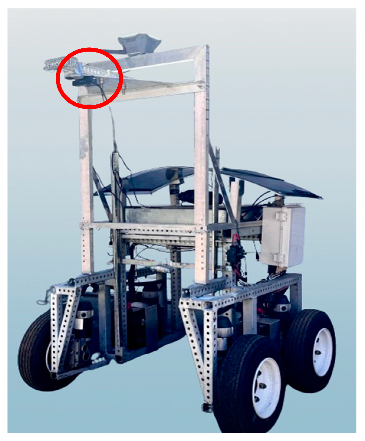
The depth camera was equipped with an RGB camera in the middle along with two monochromatic cameras on the sides for stereovision (Figure 2). The camera was installed on the front of the UGV at a height of 1.5 m above the ground surface using an aluminum frame, as shown in Figure 3. This installation height was selected based on the minimum depth measurement range of 0.7 m for the depth camera. The camera’s effective area of coverage (AOC) for stereovision as per the horizontal and vertical field of view (FOV) of 72° and 49° are 2.1 m and 1.3 m. It was calculated using the FOV calculator by the manufacturer [29], and thus, the camera covered an area of 2.7 m².

However, this FOV covered some non-plant regions like UGV tires and frames, so the effective FOV used for the study was cropped during the data-capturing stage. The depth camera was powered using the co-axial power connectors, connected to the 12 V battery installed on the UGV.

2.3. Data Collection Procedures

2.3.1. Measurement of Crop Height and Vegetation Coverage

The two monochromatic cameras were used to measure crop height. These cameras worked on the principle of stereovision. They measured the distance from the crop canopy based on the disparity in the image views between the two stereo cameras. This camera had the potential to measure the distance for every pixel in its field of view and hence provided the crop height at all these pixels in the effective FOV. The central region of the effective FOV was used for data acquisition to eliminate any possible edge-effect errors.

The UGV equipped with the depth camera was driven over the marked plots to measure the distance of the camera from the crop canopy every second. The UGV was operated at a speed of 0.6 m/s, which allowed it to capture 8 data points in a 4.57 m long plot. The UGV was also mounted with Emlid Reach RS+ as the rover station which recorded the real-time corrected geolocation. An ASUS TUF A15 Gaming Laptop (ASUSTeK Computer Inc., Beitou District, Taipei, Taiwan) with Ryzen 7 4800H mobile processor, 16 GB RAM and 512 GB storage was used to extract the data from the depth camera and RS+ via USB 3.2 Gen-1 Type-A ports.

The distance measurements from the depth camera were merged with their geolocations using a Python script. For measuring the vegetation coverage, the RGB camera (Figure 2) was used to capture the images of the crop canopy. The RGB image and crop height data were captured at the same geolocation and instant to eliminate any error caused by temporal delay.

2.3.2. Postharvest Field View with UAV

The DJI Mavic Pro (SZ DJI Technology Co. Ltd., Nanshan, Shenzhen, China) was used with a Survey 3W RGB camera (Mapir Inc., San Diego, CA, USA) to capture the aerial images of the field. This was performed with a pre-planned flight mission using the Drone Deploy website (https://www.dronedeploy.com; accessed: 16 May 2024) over the experimental site. The flight parameters are shown in

Table 3. UAV flight parameters.

Parameter	Details
Flight altitude (m)	18.29
Front overlap (%)	75
Side overlap (%)	75
Flight speed (m/s)	1.8 (Auto Set)
Perimeter 3D	ON
Crosshatch 3D	ON

. Other settings were either preset or were kept by default. These UAV images were used for generating the orthomosaics of the harvested field for serving the following purposes:

• To identify the region of interest (harvested areas) for post-processing and eliminating the non-relevant data.
• To geolocate the plots in the field based on the coordinates measured with RTK-GPS.
• To measure the exact harvested area of the plots excluding the non-harvested regions of marked plots.

2.4. Challenges in Data Collection and Solutions

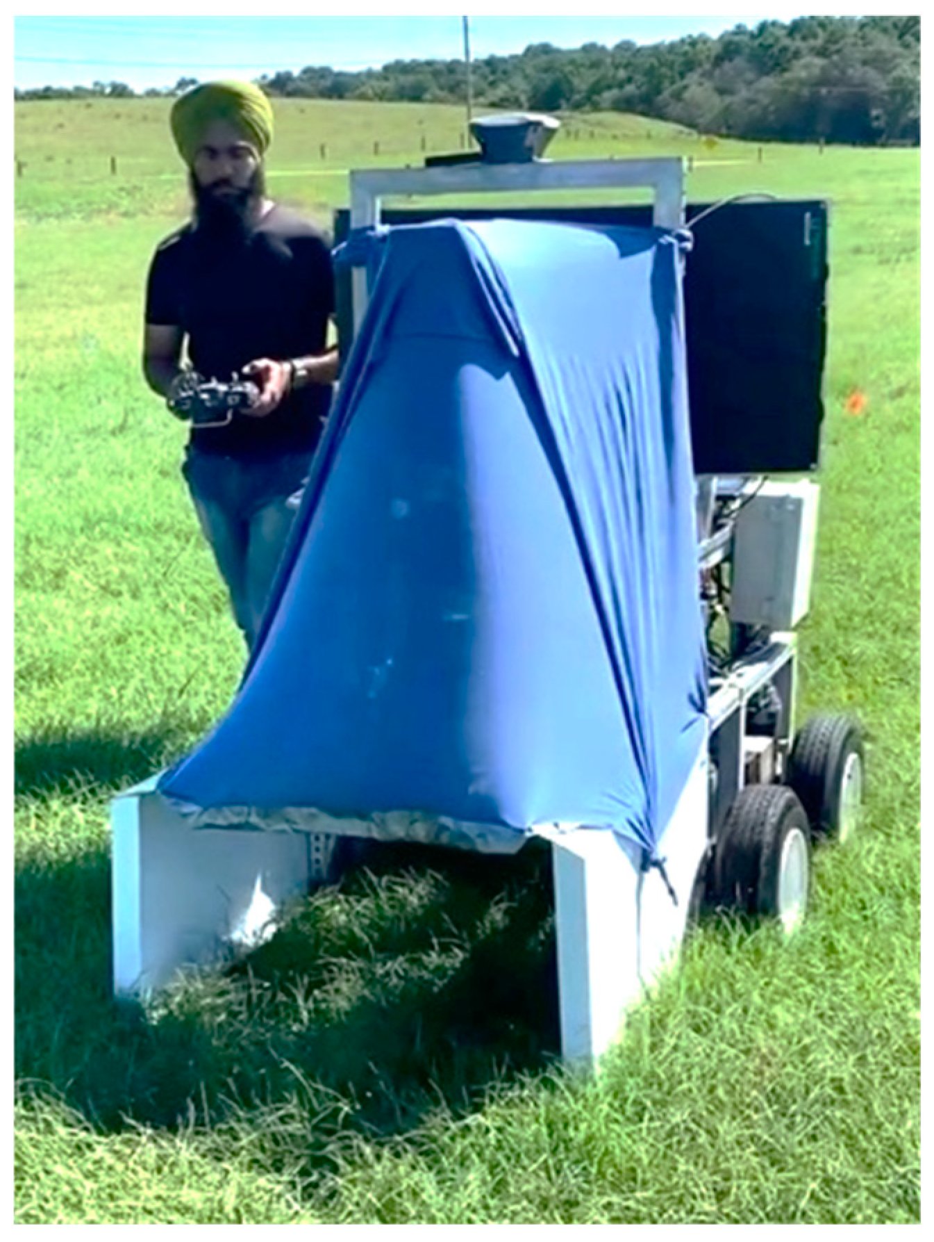
While testing the depth camera in the field, it was observed that the sunlight exposure on the AOC was causing an error in the height measurements. To solve this issue, the UGV was mounted with two aluminum side shades on the left and right sides of the AOC. A cloth cover was also attached on the top extending from the camera mount to the aluminum side shades. The aluminum was selected to make the shades rigid enough to prevent them from becoming damaged in the field while colliding with the crop canopy.

The cloth cover was used to allow an optimal amount of diffused light inside the covered region to capture the RGB images. The aluminum and cloth shade installed on the UGV are shown in Figure 4. Additionally, some plots (n = 5) in the field missed the data capturing since the laptop that was recording the data was accidentally switched off. Hence, the total number of plots with available data was reduced to 131.

2.5. Harvesting and Weighing of Plots for Wet Biomass Yield Calculations

After capturing the height data and RGB images, the marked plots were harvested using the employed harvesters. The weight measurements of the harvested forage were simultaneously recorded in the field using the onboard weighing scale of the plot harvester. For lawn mower harvesting, a battery-operated weighing scale (Measuretek Enterprise Ltd., Richmondhill, CA, USA) was used. These weight measurements resulted in providing the wet biomass yield (WBY) (kg-wet/ha) in every plot. The plots were harvested at an average height of 5.08 cm. However, due to field’s topography and presence of anthills, the harvesting height was increased to 6.35 cm to avoid the inclusion of soil or anthills in the harvested forage during the harvesting and collection in the case of the plot harvester. For the lawn mower, these issues were not encountered; therefore, a constant cutting height of 5.08 cm was maintained.

2.6. Plot Subsampling for Dry Matter Calculations

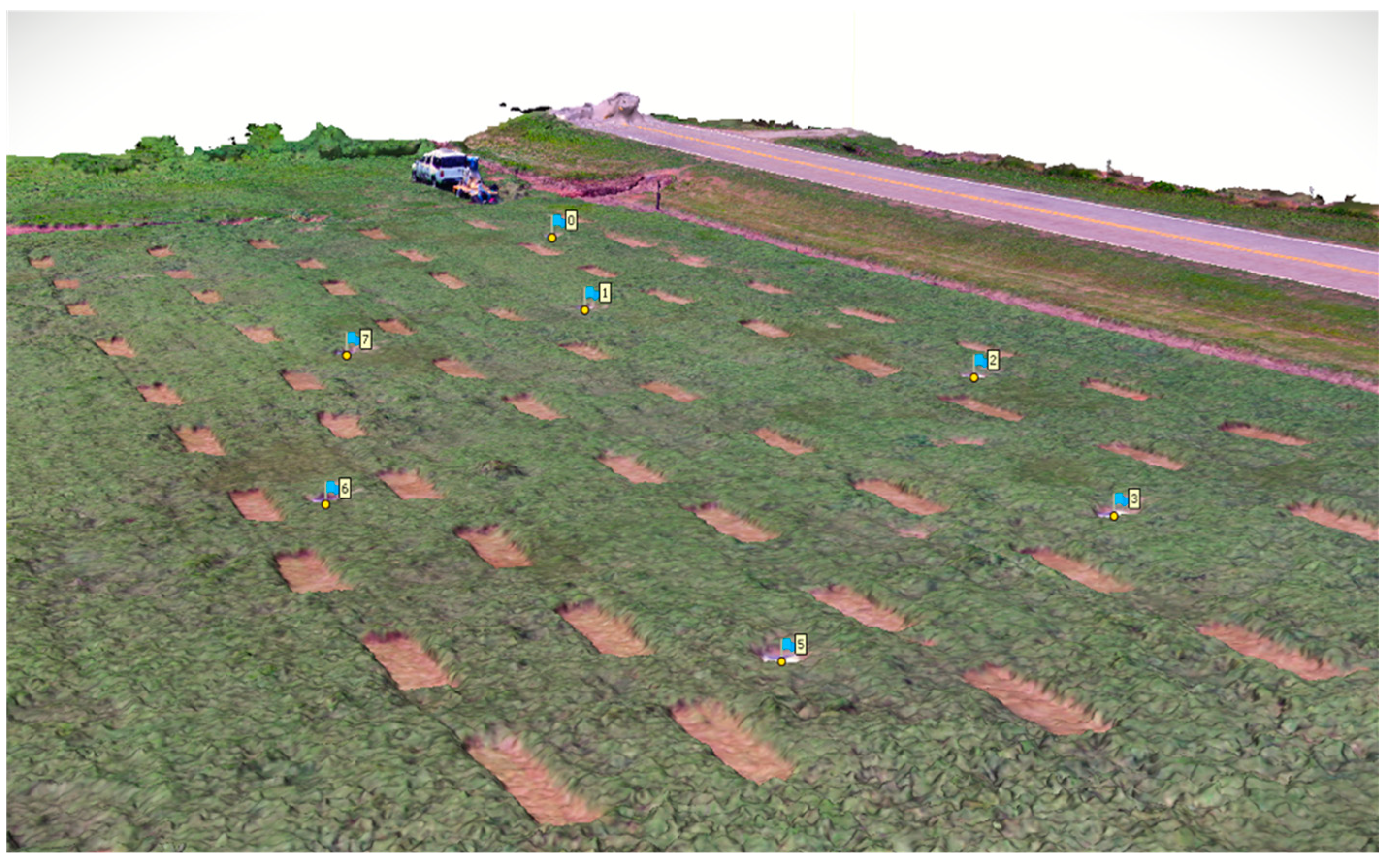
To obtain the dry matter fraction (DMF), the sub-samples from each plot (131 harvests) were collected after harvesting and stored in Ziplock bags. These collected samples were taken to the laboratory and dried at 55 °C (forced air oven) for 48 h to determine the DMF for every harvested plot sample. The DMF values were used to derive the dry biomass yield (DBY) predictions. The 3D model view of the harvested plots is shown in Figure 5.

2.7. Post-Processing of Recorded Data and Development of Prediction Function

The post-processing of the raw data captured in the form of aerial RGB images, coordinates, crop heights, and images for vegetation coverage were conducted in various software programs. The detailed post-processing steps for each raw data category and software are explained below.

2.7.1. Generating Orthomosaics from UAV RGB Images

The images captured with the UAV-mounted Survey 3W camera were imported to Agisoft Metashape Pro 1.8.3 (Agisoft LLC, St. Petersburg, Russia) photogrammetry software for generating the orthomosaics. Initially, the images were aligned according to the manually georeferenced GCPs, in Metashape, followed by the creation of a dense cloud, mesh, DEM, and orthomosaic. Every image imported to the software was geotagged with reference to these GCPs to align the generated orthomosaic with the real-world coordinates. The preset parameters for each of these steps were kept at default selections and all models were generated at a high quality and with moderate filtering settings.

After the completion of the photogrammetry process, the orthomosaics were exported as a TIFF file. These orthomosaics were later imported to ArcGIS Pro 3.2.2 (ESRI, Redlands, CA, USA), where a polygon layer was created around the boundaries of each harvested plot manually, ensuring that it outlined only the harvested regions of the plot. This layer was used to calculate the actual harvested area for each plot, excluding the unharvested/missed region in the plots, which do not contribute to biomass. This harvested area was used in the aboveground wet biomass (kg-wet/ha) calculations by dividing the measured mass of the harvested forage (kg) with the harvested area of each plot (ha). The geolocation of the center of the plots that were recorded with RTK-GPS helped ensure the location of every plot in the real world. This polygon layer was also used as the spatial boundary of the ROI for calculating the crop height and vegetation coverage for every plot.

2.7.2. Extraction of Crop Height from Raw Data

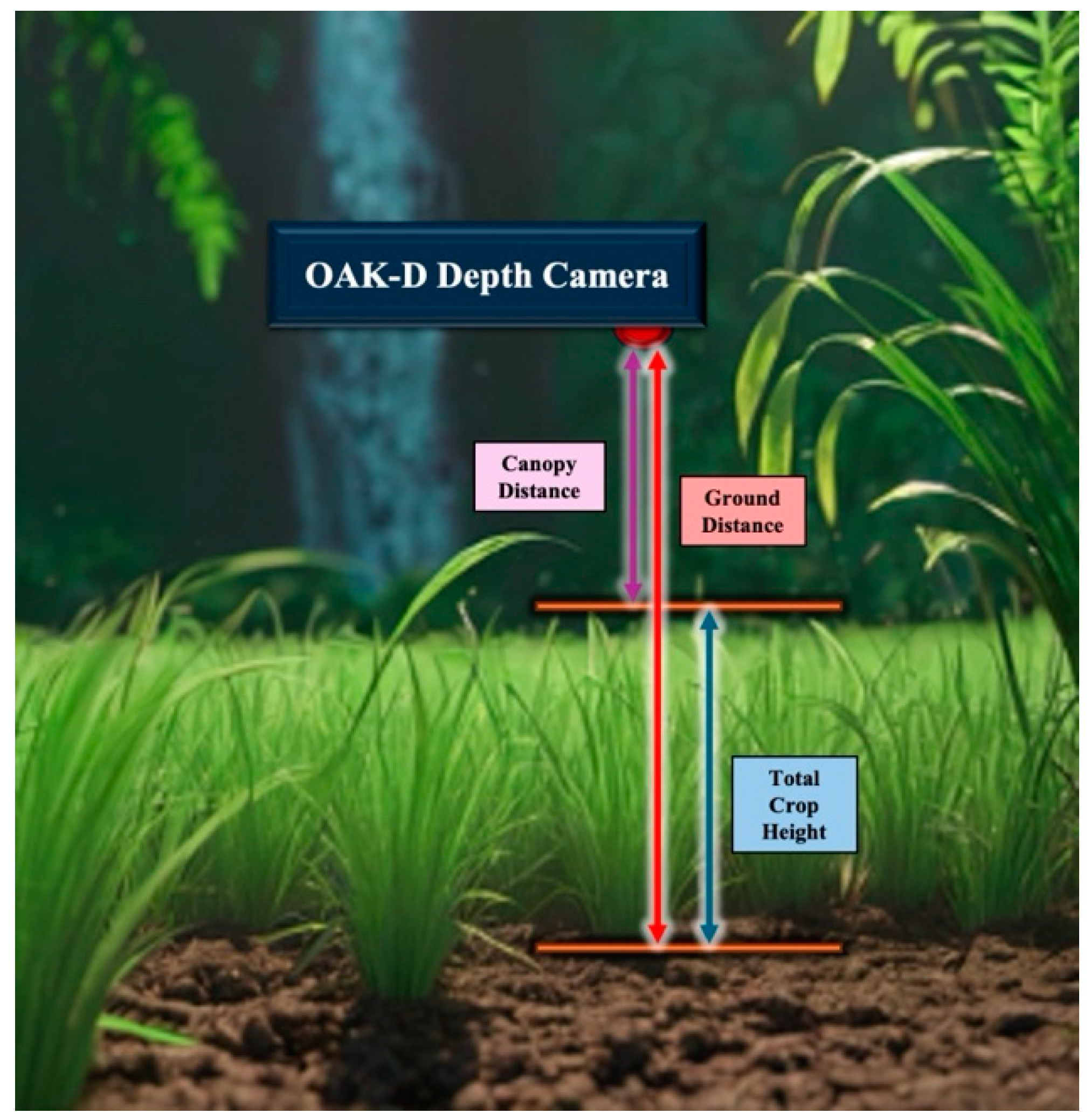
The raw data collected in the field contained the coordinates (Latitude, Longitude), date, time, and the canopy distance values measured using the depth camera. These were imported into ArcGIS Pro 3.2.2 as a point layer, and the plot boundary layer described in Section 2.7.1 was used as a mask for this point layer. All the data points falling into the boundary of the plots were considered as the relevant data for the statistical calculations. The mean values of canopy distances were used to represent that plot. The mean canopy distance was subtracted from the ground distance to obtain the total crop height (TCH) as shown in Figure 6. Next, the height at which the crop was harvested, i.e., the cut canopy height (CCH), was subtracted from the TCH to obtain the height of the actual harvested crop in the field; this is defined as the change in crop height (∆H).

2.7.3. Vegetation Coverage from RGB Images

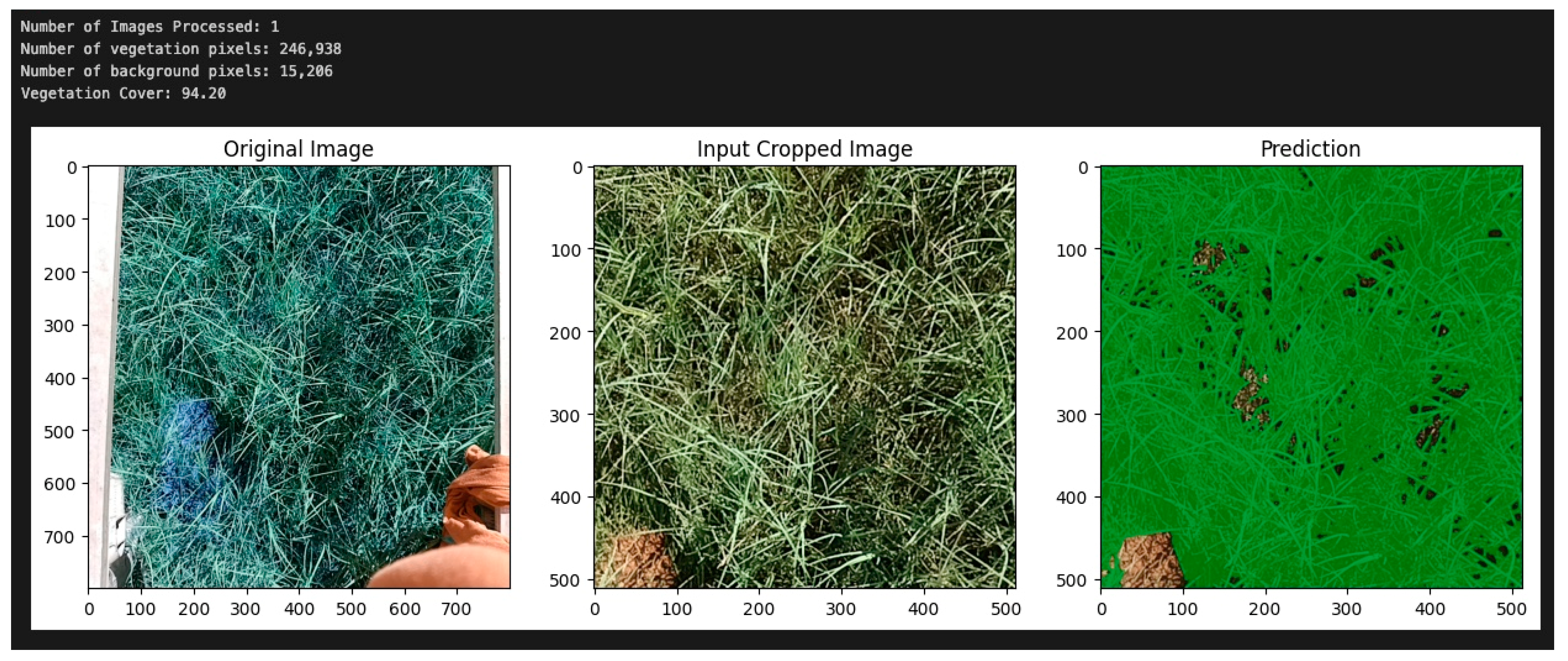
The RGB images captured with the depth camera were processed through a pre-trained Neural Network-based pixel segmentation machine learning (ML) model called SegVeg, developed and trained by Serouart et al. [30]. This program utilized the U-Net model for segmenting vegetation from the background (generally soil) and later used support vector machines (SVM) for segmenting green and senescent vegetation. For this study, only the vegetation versus background segmentation was performed. The segmentation results were later converted to obtain the percent of green vegetation in each image, which is called the VC. These data, along with the coordinates of every RGB image, were imported into ArcGIS Pro 3.2.2, and in a similar manner to the TCH, the VC values were also statistically summarized to obtain a mean VC for each plot. The segmented image illustration is shown in Figure 7. It was observed that some of the darker vegetative regions in the captured images were identified as the background by the system. These darker regions were the results of the non-uniform illumination of the area of coverage and thus might impact the aboveground yield predictions. The prediction results from the vegetation coverage were compared with the existing studies to evaluate the impact of these issues on the predictions and to investigate the ability of the VC as an independent variable to predict the aboveground biomass yield.

2.7.4. Development of the Prediction Function

The exporting of the data files, described in Section 2.7.1 and Section 2.7.2 for the ∆H and VC, respectively, were merged; these included the date, plot number, TCH, CCH, ∆H, VC, DMF, WBY, and DBY from both the harvested sections. The WBY prediction functions were developed from the ∆H, VC, and the combined ∆H and VC as potential independent variables using linear regression analysis. The general equation of the developed prediction function is shown in Equation (1):

β_w = b₁ × ∆H + b₂ × VC + c.

(1)

where,

β_w = wet biomass yield (kg-wet/ha);

b₁ = coefficient of change in crop height;

∆H = change in crop height (mm);

b₂ = coefficient of vegetation coverage;

VC = vegetation coverage (%);

c = y-intercept (kg-wet/ha).

The crop height accounts for the vertical growth of the forage above the ground and, hence, contributes significantly to the biomass. Similarly, vegetation coverage explains the crop spread across the field. The higher crop height and vegetation coverage values show high biomass availability in the field. But, if the crop height or vegetation coverage is zero, it conveys that no crop is available in the field for harvesting. So, the biomass amount with respect to that should also be zero. Therefore, the prediction function generated for biomass quantification must pass through the origin, justifying zero biomass at zero vegetation coverage and crop height. Thus, the β_w(∆H), β_w(VC), and β_w(∆H, VC) were generated with both approaches, i.e., with the y-intercept (c ≠ 0) and the intercept set through the origin (c = 0). The results from these prediction functions were statistically evaluated to conclude the best approach. Next, the β_w was multiplied by the mean DMF from all the plots to obtain the dry biomass yield predictions, as shown in Equation (2).

β_d = DMF_m × β_w.

(2)

where,

β_d = dry biomass yield (kg-DM/ha);

DMF_m = mean dry matter fraction;

β_w = wet biomass yield (kg-wet/ha).

3. Results and Discussion

3.1. Correlation Analysis

The results for the β_w (c ≠ 0) indicated a positive correlation of the independent variables with the WBY. Highly significant correlation coefficients (p < 0.001) of 0.62 for the β_w(∆H), 0.43 for the β_w(VC), and 0.65 for the β_w(∆H,VC) were observed. However, despite the significant correlation, the coefficient of determination was too low to be of practical use, given none of these relationships described even half (0.50) of the variability in β_w (

Table 4. Results from correlation and regression analyses for β_w(∆H), β_w(VC), and β_w(∆H, VC).

	βw(∆H)	βw(VC)	βw (∆H, VC)
Average WBY (kg-wet/ha)	5585	5585	5585
n	131	131	131
R2 (c ≠ 0)	0.38	0.18	0.42 *
R2 (c = 0)	0.91	0.89	0.92 *
p-value of regression (c = 0)	p < 0.001	p < 0.001	p < 0.001
SeY (kg-wet/ha)	1824	2040	1726
CV	33%	37%	31%
b1	38.38	0	25.07
p-value (b1)	p < 0.001	NA	p < 0.001
95% confidence interval (b1)	±2.11	NA	±6.85
b2	0	72.76	26.36
p-value (b2)	NA	p < 0.001	p < 0.001
95% confidence interval (b2)	NA	±4.47	±12.96

* Adjusted R², NA: Not Applicable.

).

However, setting the intercept through the origin (c = 0) showed a drastic improvement in the R² value. It increased to a minimum of 0.89 for the β_w(VC) and to a maximum of 0.92 for the β_w(∆H,VC). All these correlations were highly significant (p < 0.001) and indicated a stronger positive correlation, compared to the prediction functions with the y-intercept (c ≠ 0).

This approach with the zero-intercept was also adopted by Flombaum and Sala [26] in their research, who supported its justifications for similar applications. The zero-intercept compensates for the unknown information about the other unmeasured crop properties that influence the biomass quantity. Thus, the further regression analysis for all the independent variables was based on a similar approach (c = 0).

3.2. Regression Analysis

3.2.1. ∆H as the Independent Variable (β_w(∆H))

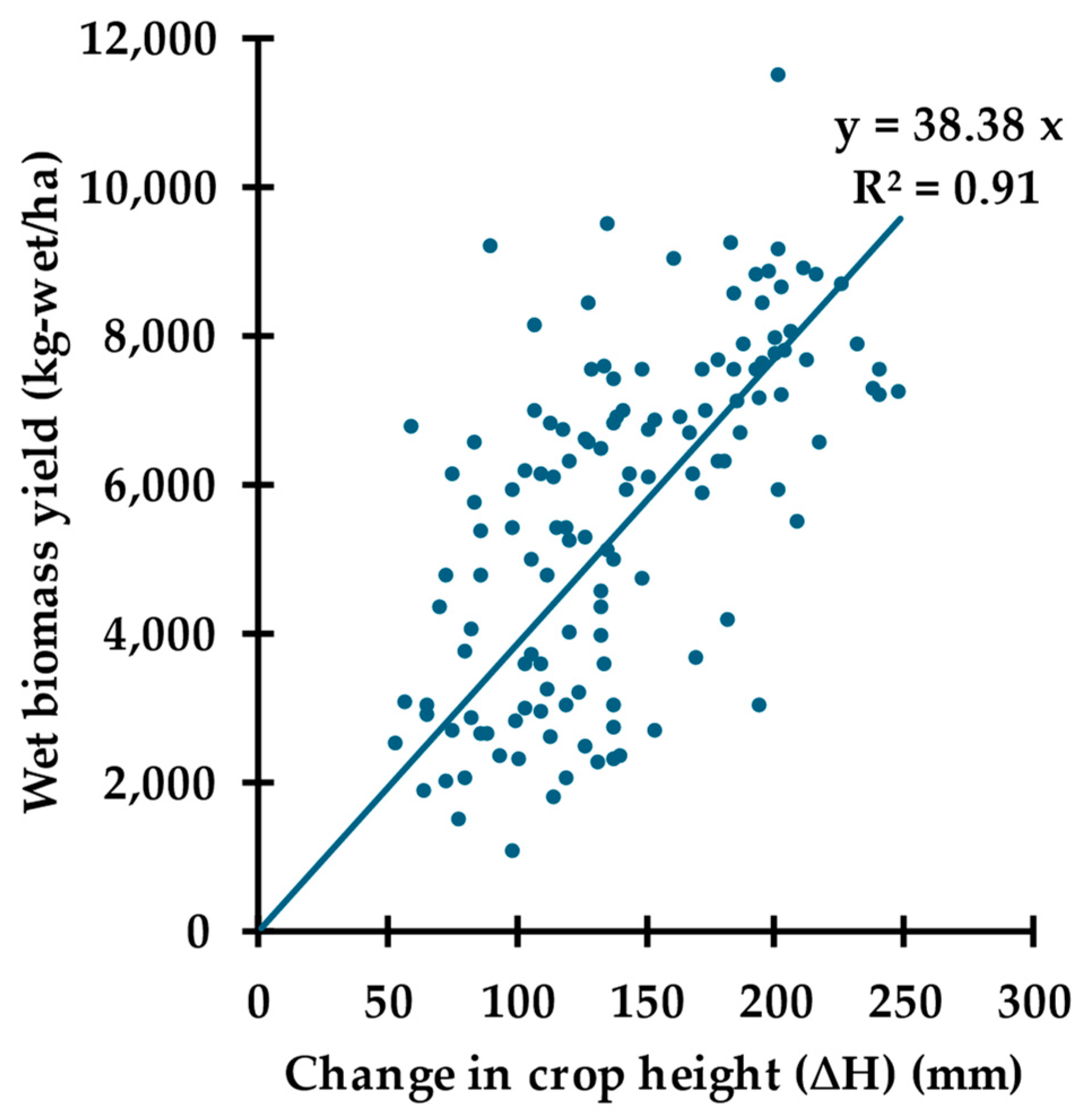
The regression results for the β_w(∆H) indicated the standard error of the β_w estimates (SeY) was 1824 kg-wet/ha, with a coefficient of variation (CV) equal to 33%. The coefficient, b_1, of the independent variable (∆H) was 38.38, with a 95% confidence interval of ±2.11. These findings suggest that the change in crop height can explain 91% of the variability in the β_w (R² = 0.91) with a highly significant linear relation (p < 0.001). The visual representation of the regression results for β_w(∆H) is shown in Figure 8.

3.2.2. VC as the Independent Variable (β_w(VC))

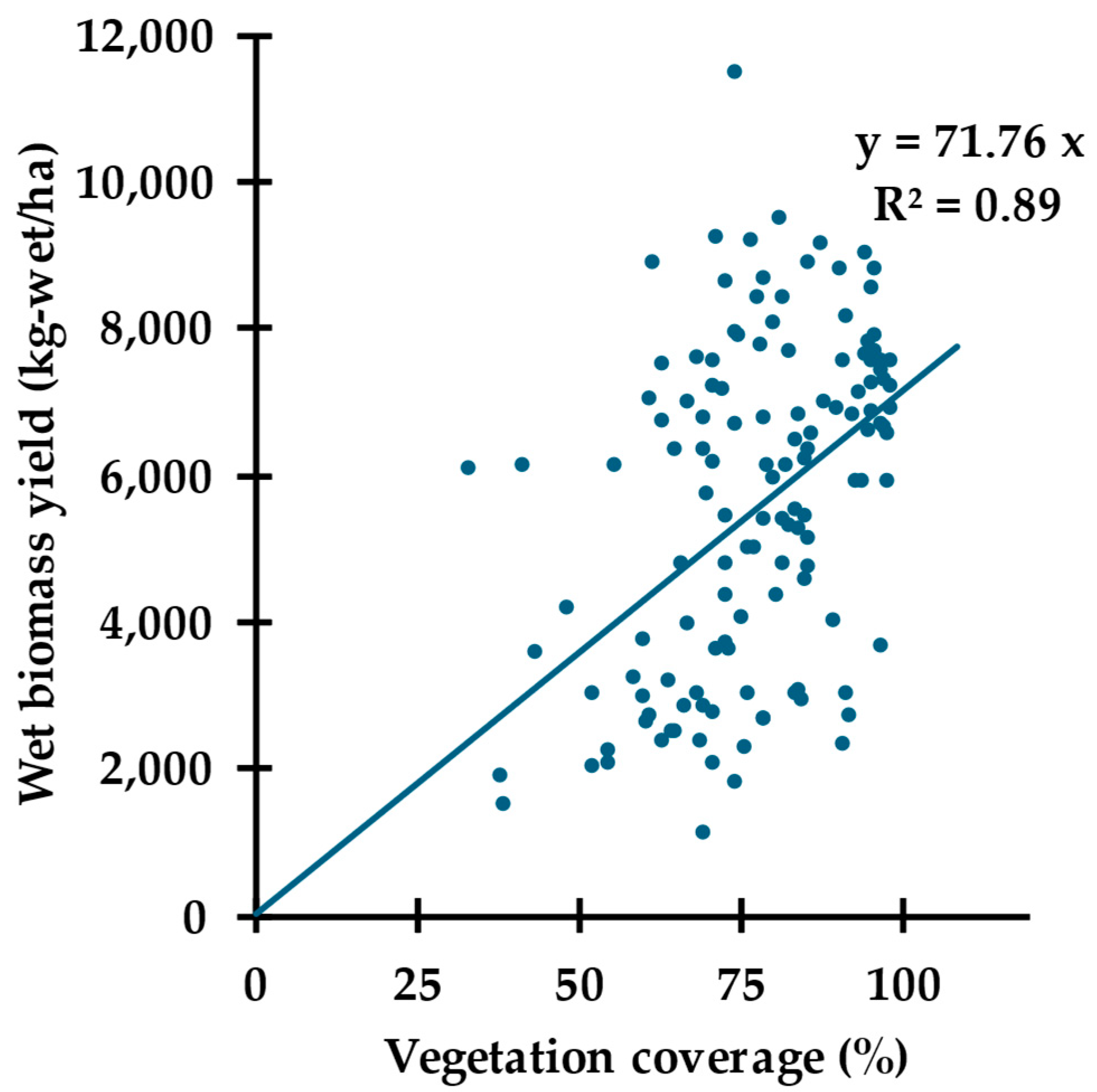
The prediction function for the VC produced an R² value of 0.89 (Figure 9). The SeY was 2040 kg-wet/ha with a 37% CV. A highly significant regression coefficient, b₂, of 71.76 ± 4.47 was observed for the β_w(VC) with a 95% confidence interval. The results indicate that the VC can satisfactorily explain 89% of the variability in the β_w.

3.2.3. Compare and Contrast between the β_w(∆H) and β_w(VC)

It can be inferred from Table 4 that the R² value was higher (0.91) in the case of the β_w(∆H) compared to the β_w(VC), which produced an R² value of 0.89. The lower SeY of 1824 kg-wet/ha was observed for the β_w(∆H) compared to the β_w(VC) with SeY of 2040 kg-wet/ha. The CV was also lower for the β_w(∆H) (33%) compared to the β_w(VC) (37%). In addition to that, as shown in Figure 8, it was observed that the data points were evenly scattered around the line of best fit over the range of measurement for the β_w(∆H). But in the case of the β_w(VC), a skewness in the data point spread was observed around the extremes (Figure 9). For the VC values less than 75%, the function overpredicts the β_w(VC), and for the VC above that, it tends to underpredict the estimates.

Therefore, to obtain additional insight into what was observed from the graphs, the mean residual of three observations at the upper and lower extremes for both the prediction functions were compared. The results indicated that the mean residual for the β_w(VC) was 4585 kg-wet/ha at the upper extreme and 2955 kg-wet/ha at the lower extreme. As expected, these residuals were higher than the β_w(∆H), with a mean residual of 3418 kg-wet/ha at the upper extreme and 2297 kg-wet/ha at the lower extreme. Notably, the higher residuals imply a higher deviation of the β_w from the observed values, indicated by the skewness in Figure 9. This could be an impact of the darker regions in the captured images due to a non-uniform illumination in the area of coverage. This might have resulted in the error in the VC calculation from the RGB images, whose possible impact is visible as the skewness in the data point scatter.

Thus, the above results indicate that the β_w(∆H) was better than the β_w(VC) in all aspects for WBY predictions. This favors the β_w(∆H) as a standalone method for yield estimation in bermudagrass when using a single independent variable. This result is also supported by several other researchers who used crop height as an independent variable for biomass quantification in various crops and achieved satisfactory results of its correlation [31,32,33]. As shown in Table 1, compared to the results from various studies on biomass estimation, the prediction functions developed in this study using the ∆H and VC showed higher values of the coefficient of determination (R²). This also conveys that despite the darker regions being identified as the background pixels, the results from the β_w(VC) were satisfactory and better compared to the related studies (Table 1), indicating the least impact of the observed issue. However, the discussed issue needs to be resolved for further applications and attaining better results.

3.2.4. Incorporation of ∆H and VC into a Multiple Linear Regression Function (β_w(∆H, VC))

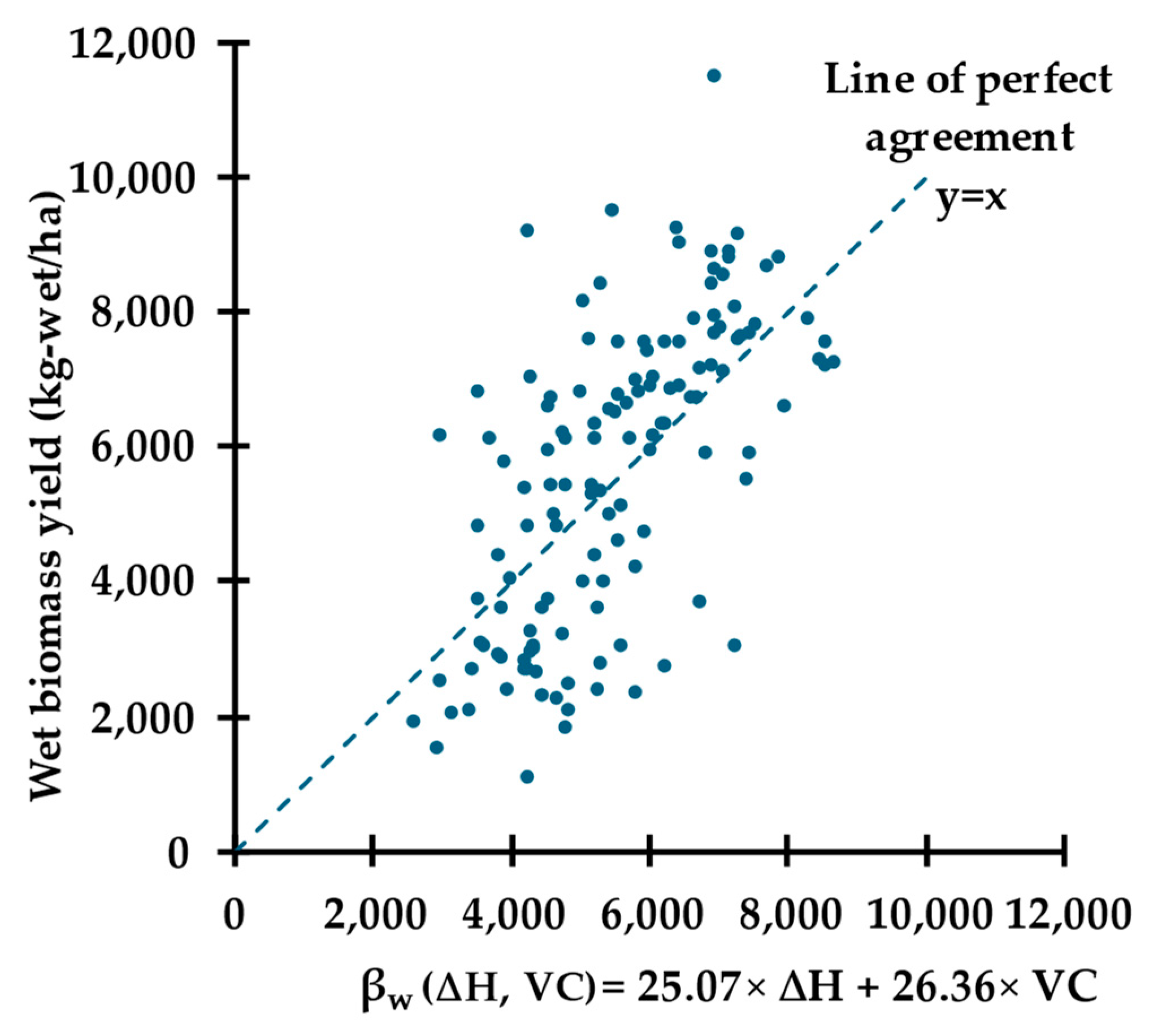
The regression analysis between the observed vs predicted biomass values for the β_w(∆H, VC) was conducted, which produced an R² value of 0.92. The SeY of 1726 kg-wet/ha and a CV equal to 31% were also observed for the combined prediction function. The coefficients of the independent variables, b₁ and b₂, in the multiple linear regression function were highly significant (p < 0.001), indicating an acceptable performance of the prediction function for wet biomass estimation. The WBY vs. β_w(∆H, VC) scatter, along with the line of perfect agreement (y = x), is shown in Figure 10.

3.2.5. Impact of Combining VC with ∆H on β_w Performance (β_w(∆H) vs. β_w(∆H, VC))

Since the R² value was high for both the β_w(∆H) and the β_w(VC), the next step was to determine if the β_w(∆H, VC) was superior to the β_w(∆H). The results showed that the β_w(∆H, VC) achieved the highest R² value (0.92) and the lowest SeY (1726 kg-wet/ha) compared to the β_w(∆H) (Table 4). The CV (31%) was also less, indicating that the β_w(∆H, VC) performed better than the β_w(∆H). However, after evaluating the magnitude of this improvement, it was seen that the R² value incremented by just 0.01 and the CV decreased by 2% only. The SeY became reduced by only 98 kg-wet/ha compared to the β_w(∆H). These improvements were, however, significantly smaller in magnitude, compared to the average WBY from all the harvests.

Additionally, an artifact of the skewness in the β_w(VC) was observed after combining the VC with ∆H in the β_w(∆H, VC), which can be seen in Figure 10. This skewness might influence the accuracy of the WBY prediction in the combined prediction function. This was confirmed by comparing the residuals for the β_w(∆H) and β_w(∆H, VC) at the upper and lower extremes. A higher magnitude of residuals was observed in the β_w(∆H, VC) (upper = 3713 kg-wet/ha, lower = 2606 kg-wet/ha) as compared to the β_w(∆H) prediction function. This signifies a higher deviation of the β_w(∆H, VC) from the WBY values compared to the β_w(∆H).

Therefore, the above results indicate the preferability of the β_w(∆H) over the β_w(∆H, VC) as a function for WBY estimation. Additionally, dealing with only one independent variable (β_w(∆H)) helps in the reduction of cost, labor, time, and data processing complexities, over the β_w(∆H, VC), without significantly compromising the prediction results. The recommended prediction function, β_w(∆H), is defined in Equation (3) and was used for deriving the DBY along with the DMF values.

β_w (∆H) = 38.38 × ∆H.

(3)

3.3. Dry Matter Fraction

All the plots were sub-sampled after harvesting, and the DMF values for each plot (n = 131) were measured. It was observed that the CV for the DMF across all the harvests was 23%. The mean DMF was 0.44 with a standard deviation of 0.10. This indicates a large variation in the DMF between harvests. Dore [34] observed that the average DMF for bermudagrass is around 0.41 for 42 days of growth with a minimum and maximum of 0.22 and 0.50, respectively. Therefore, the DMF value in this study was within the typical range. The common practice for calculating the DBY is multiplying the WBY values with the DMF. The mean DMF (DMF_m) from 131 harvests was multiplied with the β_w for each plot to obtain the β_d, as indicated in Equation (2). Zhang et al. [32] also used average dry matter to obtain the dry biomass yield in maize.

3.4. Prediction of Dry Biomass Yield (β_d)

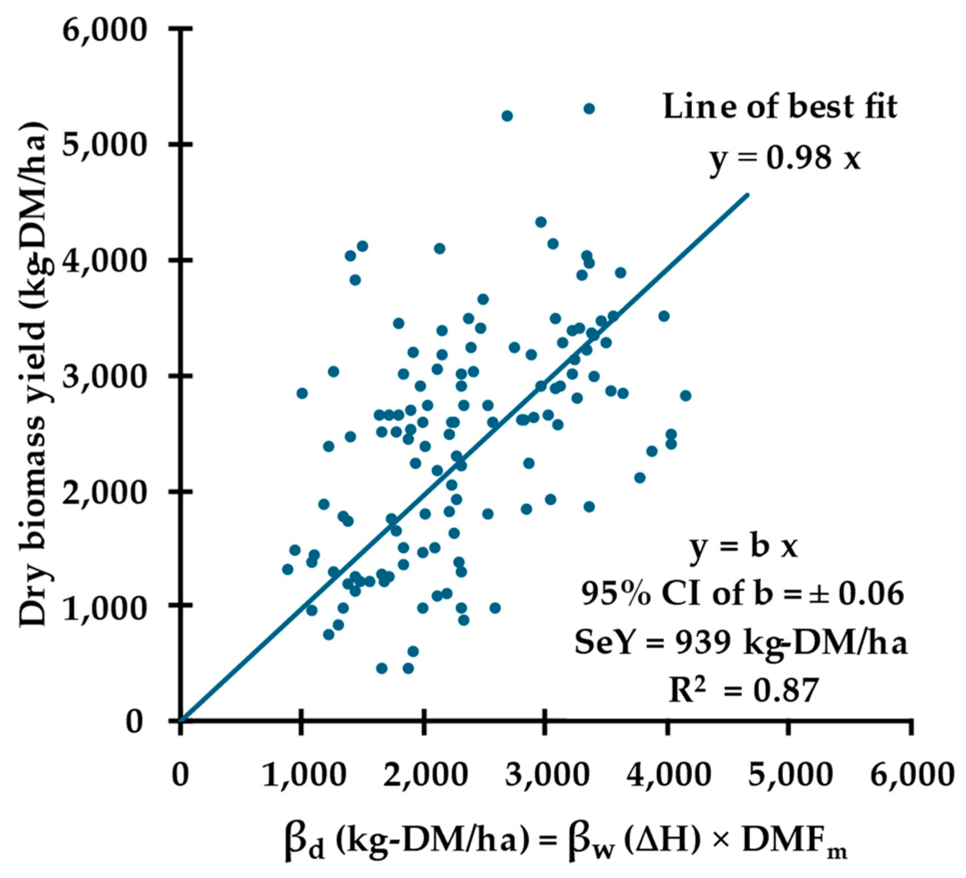
The recommended prediction function, β_w(∆H) (Equation (3)), was used as a function to derive the β_d(∆H) values using the mean DMF, as per Equation (2). A linear regression between the β_d and DBY values was used to generate the equation for the line of best fit (y = bx). The line of best fit was compared with the line of perfect agreement (y = x) to evaluate the performance of the β_d(∆H). The line of perfect agreement would have a slope of 1. The prediction function equation (line of best fit) and results from the regression analysis are illustrated in Figure 11.

It was observed that the line fitting through the observed vs. predicted dry biomass yield (line of best fit) had a slope of 0.98, which was not significantly different from the slope of the line of perfect agreement (slope = 1). Moreover, the 95% confidence interval of the variation in the slope was ± 0.06. This indicates the upper and lower bound of the slope (b) as 1.04 and 0.91, respectively. Notably, the slope of the line of perfect agreement (b = 1) falls into this 95% CI range. Therefore, the β_d(∆H) illustrated a satisfactory performance, with the standard error of 939.52 kg-DM/ha for DBY estimates. The regression showed an R² value of 0.87. This additional error and decrease in the coefficient of determination (R²) was endorsed by using the mean DMF of all harvests, for varying DMF values across the field.

These results justify the applicability of the ∆H as the independent variable to estimate aboveground WBY (kg-wet/ha) and the suitability of the wet biomass function, β_w(∆H), to estimate the β_d using the DMF_m. In the study by Koc et al. [35], the seasonal average of the DMF for Alfalfa was used to make the DBY predictions for each harvesting season. However, the approach practiced in this research is also recommended for making the DBY estimates. Even if the knowledge of the DMF is enhanced, using any suitable method, the maximum coefficient of determination that can be achieved will be 0.91 if the developed function of ∆H (β_w(∆H)) for the β_d estimation is used.

4. Conclusions

This research focused on the implementation of stereovision for crop height measurement in bermudagrass. The influence of the crop height and ML-based vegetation coverage was studied for biomass estimation. The findings convey the strong ability of stereovision as a crop height measurement system. The impactful representation of crop height for explaining the variability in the aboveground biomass supports the method. It was observed that both the ∆H and VC highly correlate with the WBY. However, the ∆H provided the best prediction equation if one independent variable was used.

Combining the ∆H and VC provided slightly improved results, but the scatter about the regression line was not uniform. This improvement was minimal in contrast to the time, labor, and resources involved in extracting the vegetation coverage. Thus, for the development of the ground rover, which can predict the aboveground biomass, stereovision can be a useful method for measuring crop height.

Recording a greater number of data points is suggested as part of future studies while using stereovision-based crop height and vegetation coverage as predictors. This might help to increase the system’s adaptability among variable environments and crop diversities. A system to measure the real-time dry matter content of the crop canopy can be helpful in improving dry biomass predictions. For improving the performance of the VC, it is suggested to use a higher resolution camera for capturing the canopy images. It is also recommended to develop a personalized ML model for segmenting vegetative and non-vegetative pixels, specifically for grasses. This will focus on a specific crop architecture and may produce enhanced results. Additionally, it is suggested to use a built-in light source for the illumination of the area of coverage. It should be accompanied by an opaque shading surface to block diffused sunlight and thus eliminate its effects on data recording. This artificial light source might help in illuminating the darker vegetative regions for better data capturing and the post-processing of the RGB images.

References

1. Squires, V.R.; Dengler, J.; Feng, H.; Hua, L. Grasslands of the World: Diversity, Management and Conservation; A Science Publishers Book: Boca Raton, FL, USA, 2018. [Google Scholar]
2. Hansen, T.; Mammen, R.; Crawford, R.; Massie, M.; Bishop-Hurley, G.; Kallenbach, R. Agriculture MU Guide- MU Extension, University of Missouri-Columbia. Available online: https://extension.missouri.edu/publications/g4620# (accessed on 28 May 2024).
3. Drewitz, N.; Goplen, J. Measuring Forage Quality|UMN Extension. Available online: https://extension.umn.edu/forage-harvest-and-storage/measuring-forage-quality (accessed on 2 January 2024).
4. Whitbeck, M.; Grace, J.B. Evaluation of non-destructive methods for estimating biomass in marshes of the upper Texas, USA coast. Wetlands 2006, 26, 278–282. [Google Scholar] [CrossRef]
5. Li, C.; Wulf, H.; Schmid, B.; He, J.S.; Schaepman, M.E. Estimating plant traits of alpine grasslands on the qinghai-tibetan plateau using remote sensing. IEEE J. Sel. Top. Appl. Earth Obs. Remote. Sens. 2018, 11, 2263–2275. [Google Scholar] [CrossRef]
6. Semela, M.; Ramoelo, A.; Adelabu, S. Testing and Comparing the Applicability of Sentinel-2 and Landsat 8 Reflectance Data in Estimating Mountainous Herbaceous Biomass before and after Fire Using Random Forest Modelling. In Proceedings of the International Geoscience and Remote Sensing Symposium (IGARSS), Waikoloa, HI, USA, 26 September–2 October 2020; pp. 4493–4496. [Google Scholar] [CrossRef]
7. Meshesha, D.T.; Ahmed, M.M.; Abdi, D.Y.; Haregeweyn, N. Prediction of grass biomass from satellite imagery in Somali regional state, eastern Ethiopia. Heliyon 2020, 6, e05272. [Google Scholar] [CrossRef] [PubMed]
8. Fernandes, M.H.M.d.R.; Fernandes Junior, J.d.S.; Adams, J.M.; Lee, M.; Reis, R.A.; Tedeschi, L.O. Using sentinel-2 satellite images and machine learning algorithms to predict tropical pasture forage mass, crude protein, and fiber content. Sci. Rep. 2024, 14, 8704. [Google Scholar] [CrossRef]
9. Chen, Y.; Guerschman, J.; Shendryk, Y.; Henry, D.; Tom Harrison, M. Estimating Pasture Biomass Using Sentinel-2 Imagery and Machine Learning. Remote. Sens. 2021, 13, 603. [Google Scholar] [CrossRef]
10. Cho, M.A.; Skidmore, A.; Corsi, F.; van Wieren, S.E.; Sobhan, I. Estimation of green grass/herb biomass from airborne hyperspectral imagery using spectral indices and partial least squares regression. Int. J. Appl. Earth Obs. Geoinf. 2007, 9, 414–424. [Google Scholar] [CrossRef]
11. Franceschini, M.H.D.; Becker, R.; Wichern, F.; Kooistra, L. Quantification of Grassland Biomass and Nitrogen Content through UAV Hyperspectral Imagery—Active Sample Selection for Model Transfer. Drones 2022, 6, 73. [Google Scholar] [CrossRef]
12. Schulze-Brüninghoff, D.; Hensgen, F.; Wachendorf, M.; Astor, T. Methods for LiDAR-based estimation of extensive grassland biomass. Comput. Electron. Agric. 2019, 156, 693–699. [Google Scholar] [CrossRef]
13. Nguyen, P.; Badenhorst, P.E.; Shi, F.; Spangenberg, G.C.; Smith, K.F.; Daetwyler, H.D. Design of an Unmanned Ground Vehicle and LiDAR Pipeline for the High-Throughput Phenotyping of Biomass in Perennial Ryegrass. Remote Sens. 2021, 13, 20. [Google Scholar] [CrossRef]
14. Hütt, C.; Bolten, A.; Hüging, H.; Bareth, G. UAV LiDAR Metrics for Monitoring Crop Height, Biomass and Nitrogen Uptake: A Case Study on a Winter Wheat Field Trial. PFG J. Photogramm. Remote. Sens. Geoinformation Sci. 2023, 91, 65–76. [Google Scholar] [CrossRef]
15. Schaefer, M.T.; Lamb, D.W.; Ozdogan, M.; Baghdadi, N.; Thenkabail, P.S. A Combination of Plant NDVI and LiDAR Measurements Improve the Estimation of Pasture Biomass in Tall Fescue (Festuca arundinacea var. Fletcher). Remote Sens. 2016, 8, 109. [Google Scholar] [CrossRef]
16. Walter, J.D.C.; Edwards, J.; McDonald, G.; Kuchel, H. Estimating Biomass and Canopy Height with LiDAR for Field Crop Breeding. Front. Plant Sci. 2019, 10, 473161. [Google Scholar] [CrossRef] [PubMed]
17. Grüner, E.; Astor, T.; Wachendorf, M. Biomass Prediction of Heterogeneous Temperate Grasslands Using an SfM Approach Based on UAV Imaging. Agronomy 2019, 9, 54. [Google Scholar] [CrossRef]
18. Batistoti, J.; Marcato, J.; ítavo, L.; Matsubara, E.; Gomes, E.; Oliveira, B.; Souza, M.; Siqueira, H.; Filho, G.S.; Akiyama, T.; et al. Estimating Pasture Biomass and Canopy Height in Brazilian Savanna Using UAV Photogrammetry. Remote Sens. 2019, 11, 2447. [Google Scholar] [CrossRef]
19. Singh, J.; Koc, A.B.; Aguerre, M.J. Aboveground Biomass Estimation of Tall Fescue using Aerial and Ground-based Systems. In Proceedings of the 2023 ASABE Annual International Meeting, Omaha, NE, USA, 9–12 July 2023. [Google Scholar] [CrossRef]
20. Legg, M.; Bradley, S. Ultrasonic Arrays for Remote Sensing of Pasture Biomass. Remote Sens. 2020, 12, 111. [Google Scholar] [CrossRef]
21. Koc, A.B.; Erwin, C.; Aguerre, M.J.; Chastain, J.P. Estimating Tall Fescue and Alfalfa Forage Biomass Using an Unmanned Ground Vehicle. In Lecture Notes in Civil Engineering; Springer: Cham, Switzerland, 2024; Volume 458, pp. 357–372. [Google Scholar] [CrossRef]
22. Andersson, K.; Trotter, M.; Robson, A.; Schneider, D.; Frizell, L.; Saint, A.; Lamb, D.; Blore, C. Estimating pasture biomass with active optical sensors. Adv. Anim. Biosci. 2017, 8, 754–757. [Google Scholar] [CrossRef]
23. Martin, R.C.; Astatkie, T.; Cooper, J.M.; Fredeen, A.H. A Comparison of Methods Used to Determine Biomass on Naturalized Swards. J. Agron. Crop Sci. 2005, 191, 152–160. [Google Scholar] [CrossRef]
24. Shu, M.; Li, Q.; Ghafoor, A.; Zhu, J.; Li, B.; Ma, Y. Using the plant height and canopy coverage to estimation maize aboveground biomass with UAV digital images. Eur. J. Agron. 2023, 151, 126957. [Google Scholar] [CrossRef]
25. Kosmas, C.; Kirkby, M.; Geeson, N. Desertification Indicator System for Mediterranean Europe. Manual on: Key Indicators of Desertification and Mapping Environmentally Sensitive Areas to Desertification. European Commission, Energy, Environment and Sustainable Development, EUR 18882, 87 p. Available online: https://esdac.jrc.ec.europa.eu/public_path/shared_folder/projects/DIS4ME/indicator_descriptions/vegetation_cover.htm# (accessed on 2 January 2024).
26. Flombaum, P.; Sala, O.E. A non-destructive and rapid method to estimate biomass and aboveground net primary production in arid environments. J. Arid. Environ. 2007, 69, 352–358. [Google Scholar] [CrossRef]
27. Schirrmann, M.; Hamdorf, A.; Garz, A.; Ustyuzhanin, A.; Dammer, K.H. Estimating wheat biomass by combining image clustering with crop height. Comput. Electron. Agric. 2016, 121, 374–384. [Google Scholar] [CrossRef]
28. OAK-D—DepthAI Hardware Documentation 1.0.0 Documentation. Available online: https://docs.luxonis.com/projects/hardware/en/latest/pages/BW1098OAK/ (accessed on 16 May 2024).
29. Luxonis Field of View Calculator. Available online: https://fov.luxonis.com/?horizontalFov=80&verticalFov=55&horizontalResolution=1280&verticalResolution=800 (accessed on 16 May 2024).
30. Serouart, M.; Madec, S.; David, E.; Velumani, K.; Lozano, R.L.; Weiss, M.; Baret, F. SegVeg: Segmenting RGB Images into Green and Senescent Vegetation by Combining Deep and Shallow Methods. Plant Phenomics 2022, 2022, 9803570. [Google Scholar] [CrossRef] [PubMed]
31. Corti, M.; Cavalli, D.; Cabassi, G.; Bechini, L.; Pricca, N.; Paolo, D.; Marinoni, L.; Vigoni, A.; Degano, L.; Gallina, P.M. Improved estimation of herbaceous crop aboveground biomass using UAV-derived crop height combined with vegetation indices. Precis. Agric. 2023, 24, 587–606. [Google Scholar] [CrossRef]
32. Zhang, Y.; Xia, C.; Zhang, X.; Cheng, X.; Feng, G.; Wang, Y.; Gao, Q. Estimating the maize biomass by crop height and narrowband vegetation indices derived from UAV-based hyperspectral images. Ecol. Indic. 2021, 129, 107985. [Google Scholar] [CrossRef]
33. Hütt, C.; Isselstein, J.; Komainda, M.; Schöttker, O.; Sturm, A. UAV LiDAR-based grassland biomass estimation for precision livestock management. J. Appl. Remote Sens. 2024, 18, 017502. [Google Scholar] [CrossRef]
34. Dore, R.T. Comparing Bermudagrass and Bahiagrass Cultivars at Different Stages of Harvest for Dry Matter Yield and Nutrient Content. Master’s Thesis, Louisiana State University LSU Scholarly Repository, Baton Rouge, LA, USA, 2006. [Google Scholar] [CrossRef]
35. Koc, A.B.; MacInnis, B.M.; Aguerre, M.J.; Chastain, J.P.; Turner, A.P. Alfalfa Biomass Estimation Using Crop Surface Modeling and NDVI. Appl. Eng. Agric. 2023, 39, 251–264. [Google Scholar] [CrossRef]
Figure 1. Sections 1 (left) and 2 (right) (red) and plots (black) in the bermudagrass field.
Remotesensing 16 02646 g001
Figure 2. Depth camera lenses. Monochromatic stereovision cameras (blue encircled); RGB camera (green encircled).
Remotesensing 16 02646 g002
Figure 3. Depth camera mounted on UGV (red encircled).
Remotesensing 16 02646 g003
Figure 4. UGV with shades attached.
Remotesensing 16 02646 g004
Figure 5. 3D view of harvested plots generated with SfM. The flags represent the locations of the GCPs as visible in the 3D model from SfM.
Remotesensing 16 02646 g005
Figure 6. Crop height measurement.
Remotesensing 16 02646 g006
Figure 7. SegVeg pixel segmentation and extraction of VC percentage.
Remotesensing 16 02646 g007
Figure 8. Observed wet biomass yield vs. change in crop height (∆H).
Remotesensing 16 02646 g008
Figure 9. Observed wet biomass yield vs. vegetation coverage (VC).
Remotesensing 16 02646 g009
Figure 10. Observed vs. predicted wet biomass yield from the change in crop height and vegetation coverage.
Remotesensing 16 02646 g010
Figure 11. Observed vs. predicted dry biomass yield from prediction function (βw (∆H)) and mean DMF = 0.44.
Remotesensing 16 02646 g011