Temporal Transferability of Tree Species Classification in Temperate Forests with Sentinel-2 Time Series

Abstract

Detailed information on forest tree species is crucial to inform management and policy and support environmental and ecological research. Sentinel-2 imagery is useful for obtaining spatially explicit and frequent information on forest tree species due to its suitable spatial, spectral, and temporal resolutions. However, classification workflows often do not generalise well to time periods that are not seen by the model during the calibration phase. This study investigates the temporal transferability of dominant tree species classification. To this end, the Random Forest, Support Vector Machine, and Multilayer Perceptron algorithms were used to classify five tree species in Flanders (Belgium) with regularly spaced Sentinel-2 time series from 2018 to 2022. Cross-year single-year input scenarios were compared with same-year single-year input scenarios to quantify the temporal transferability of the five evaluated years. This resulted in a decrease in overall accuracy between 2.30 and 14.92 percentage points depending on the algorithm and evaluated year. Moreover, our results indicate that the cross-year classification performance could be improved by using multi-year training data, reducing the drop in overall accuracy. In some cases, gains in overall accuracy were even observed. This study highlights the importance of including interannual spectral variability during the training stage of tree species classification models to improve their ability to generalise in time.

1. Introduction

Forest ecosystems provide a wide range of functions and services related but not limited to biodiversity conservation, climate regulation, biomass production, habitat provision, and water supply. The provision of these functions and services depends on many factors, including forest type and tree species diversity [1,2]. Moreover, their provision is increasingly under pressure as forest resilience and stability are affected by stresses and disturbances [3]. In this context, knowledge about forest tree species presence and distribution is important to inform forest management and policy and supporting environmental and ecological research. For instance, detailed tree species information can contribute to the refinement of forest (soil) carbon models [4,5].

Over the past few decades, remote sensing has become a valuable tool for providing frequent and spatially explicit information on forest type and tree species composition [6,7]. Various types of remote sensing data have been successfully used for tree species classification, including very high-resolution commercial satellite imagery [8], aerial hyperspectral imagery [9,10], and aerial LiDAR data [11]. However, the high costs associated with obtaining these types of data [12,13] restrict the spatial and temporal coverage of these data and subsequently limit their operational application at large spatial and temporal scales. Passive optical multispectral satellite missions, like Sentinel-2 or Landsat, overcome these limitations and open up possibilities to create workflows that can be reproducible in time and scalable to larger areas. This potential arises from the orbital characteristics, long-term operationality, and the open and free data policy of these earth observation platforms [14,15]. Furthermore, the onboard sensors provide data with a suitable spatial, spectral, and temporal resolution. While a higher spatial resolution is required for individual tree identification and classification, a medium spatial resolution (10–60 m) has been reported to be sufficient for mapping tree species at the stand level [16]. Moreover, broadband multispectral sensors operate in the visible (VIS), near-infrared (NIR), and short-wave infrared (SWIR) wavelength regions, which are useful for differentiating tree species [17,18]. Sentinel-2 also covers the red-edge region, which has also been proven to be important for tree species classification [17,19]. Finally, a high revisit time enables the use of multitemporal data in classification approaches.

The potential of Sentinel-2 for multitemporal classification of temperate tree species has been investigated in recent studies [20,21,22,23,24,25,26,27,28,29,30]. In these studies, several coniferous and broadleaved tree species or tree species groups were classified, ranging in thematic complexity from 3 to 37 classes. Comparisons of various non-parametric machine learning methods have shown that Random Forest (RF) and Support Vector Machine (SVM) are both suitable for this application [22,23,31]. Artificial neural networks, such as Multilayer Perceptron (MLP), have been used less, but may also be useful [31]. Moreover, these studies have established that multitemporal approaches result in superior classification performance compared to unitemporal (single-date) approaches [25,27,29,30]. The general idea is that the integration of multiple acquisitions, which represent different stages of the annual phenological cycle, improves the spectral separability between tree species by capturing temporal variations in their reflectance due to changes in biophysical and biochemical attributes [32,33,34]. To take advantage of this, a key aspect is the manner in which the temporal dimension is incorporated into the classification process. Notably, the aforementioned studies have shown an evolution from using sparse and irregular time series towards more dense and regularly spaced time series. At small spatial scales, it is reasonable to select a few images from phenological key dates based on minimal cloud cover over the entire study area [20,22,26,29]. However, at larger and more complex scales, relying on cloud-free scenes is usually not feasible as it severely limits the number of suitable scenes. An alternative is the creation of best-available-pixel composites [21,23,30]. However, a few key phenological dates may not be sufficient to capture the phenological variations that are present in a larger and environmentally complex study area. Subsequent studies transitioned towards the use of more dense time series. Either all available Sentinel-2 scenes of sufficient quality (e.g., having a low degree of cloud cover) were used [25,27,28] or regularly-spaced dense time series were generated by using interpolation and/or smoothing techniques [24]. These studies usually implement a feature selection procedure to retain the most useful dates for classification. This step has been shown to be important as classification performance may saturate or even drop when more time steps are used [27,28]. Furthermore, such a feature selection step can lead to finding the most optimal input dates. However, these optimal dates are often not robust in time. For example, Karasiak et al. [28] identified the most optimal dates for tree species mapping of seven deciduous tree species in France, but those dates were not stable across different years. This can hinder the temporal transferability of trained models across years.

In remote sensing, model transferability or generalisation refers to the ability of a model to produce accurate predictions on unseen, new data outside its temporal, spatial, or spectral domain. More specifically, temporal model transferability is here defined as model transferability in the temporal domain, across satellite data captured in different years. As Gray et al. [35] point out, “When temporal generalization is attempted, classification performance is typically much lower or even unreported for time periods not captured in the training data”. Recently, this research theme has been receiving more attention, most prominently in the field of crop type mapping with studies reporting on the temporal transferability of trained models. For instance, Wijesingha et al. [36] evaluated temporal transfer scenarios and found a decrease in macro F1 score for RF from 74% to 67%. On top of that, some studies attempted to improve the temporal transferability of models by using multi-year data. For example, Kyere et al. [37] used multi-year data to train an RF model for crop type classification. The underlying idea was that the model learns different annual crop phenology patterns that help improve predictions for the other years. Using multi-year data increased the overall accuracy (OA) by six percentage points. Momm et al. [38] also evaluated a temporal model transferability scenario and found a decrease in OA from 91% to 67%. However, when using multi-year training data, an OA of 90% was achieved. The use of multi-year training data has thus been shown to be a promising route for improving temporal transferability in the context of crop type classification. In this study, multi-year training data will be investigated as a method to improve temporal transferability in the context of tree species classification.

In a forest-related context, past research has focussed on model transferability of forest structure attributes such as canopy height, stand density, and basal area across spatial regions [39] and across time periods [40,41,42]. To the best of our knowledge, there has been little research that focusses on temporal transferability in the specific context of tree species classification from multispectral satellite imagery. In this context, however, it is expected that temporally transferring a model may cause a significant drop in classification performance due to the interannual variability of spectral reflectance among remotely sensed images due to changing acquisition, atmospheric, and environmental conditions [43]. Most notably, year-to-year fluctuations in rainfall and temperature can cause shifts in species-specific tree phenology as tree species respond differently to such changes depending on their physiological requirements and adaptation potential to environmental variations [44,45,46]. For instance, the timing of dormancy can be either induced or delayed depending on the proceeding weather conditions in deciduous forests [47,48]. In general, this variability is expected to alter the relationship between the spectro-temporal input features and the target classes from year to year. Consequently, time-specific classification models may produce inaccurate predictions when they are transferred to a time period that was not captured during model calibration. Therefore, this study focusses on investigating the temporal transferability of tree species classification and the use of multi-year training data. To this end, regularly spaced Sentinel-2 time series of different years are used for dominant tree species classification of forests in Flanders. Our study addresses the following questions:

(1)

What is the predictive performance of models based on the spectral information of a single year?

(2)

How does the predictive performance of models change when a model trained on a single year is applied to the spectral information of another year?

(3)

What is the impact of multi-year training data on temporal transferability?

2. Methodology

The applied workflow, as shown in Figure 1, consists of the following components: (1) data sources, (2) data preparation, and (3) model training and evaluation. The data sources and data preparation are described in Section 2.2, while model training and evaluation are described in Section 2.3.

2.1. Study Area

This study was conducted in Flanders, the northern region of Belgium, covering a total area of 13,626 km² (Figure 2). Flanders is characterised by a temperate maritime climate. Historical land use changes have led to a severely fragmented landscape with a stable but low degree of forest cover at around 10.3% [49]. Consequently, Flanders ranks among the regions with the lowest forest area per capita in Europe [50,51]. Forests are scattered across the landscape in relatively small and diverse patches, with a higher concentration towards the east. About 10% of Flanders’ forests are smaller than 1 ha and more than 70% are smaller than 5 ha [51], resulting in a high degree of fragmentation and forest edge. About 50 years ago, regional forest policy and management started shifting its focus from wood production to forest multifunctionality, with an emphasis on the socio-cultural ecosystem services [52]. This shift has led to gradual changes in forest structure and species composition [53]. More specifically, forest structure has become more diverse in terms of age, diameter class, and vegetation structure. Moreover, the presence of standing and lying dead wood has increased. Regarding species composition, a decrease in pure conifer stands was observed in favour of mixed forest stands with an increasing presence of indigenous tree species. Based on the share of the total basal area (the sum of the cross-sectional surface area of all trees), the most common tree species in Flemish forests are Pinus sylvestris (Scots pine, 23%), Quercus robur and Quercus petraea (common and sessile oak, 14%), Pinus nigra (black pine, 10%), Populus sp. (poplar, 9%), Betula sp. (birch, 7%), Fagus sp. (beech, 6%), Quercus rubra (northern red oak, 5%), and Alnus glutinosa (common alder, 4%) [53].

2.2. Data Sources and Data Preparation

2.2.1. Reference Data

The target labels were derived from Flanders’ regional forest inventory (RFI), a policy-supporting measurement network coordinated by the Agency for Nature and Forests (ANF) of the Flemish government [55]. In this study, a combination of data from the second and third inventory cycles was used, corresponding to the data collected between 2012 and 2022 [56,57]. The potential sampling locations are systematically distributed over Flanders based on a fixed 0.5 km by 1 km grid, amounting to approximately 27,000 locations. About 10% of those locations coincide with forest cover and are visited over a period of 10 years. Consequently, the spatial distribution of the plots follows the spatial distribution of forested areas as shown in Figure 2. A continuous inventory strategy is employed to visit approximately 10% of the locations each year. The measurement plots consist of three concentric circles of varying radii. In each circle, dendrological parameters are measured for trees that meet a combined diameter at breast height (DBH) and height criterion. More specifically, in the largest circle with a radius of 18 m, all trees with a DBH larger or equal to 39 cm are measured. Additionally, in the middle circle with a radius of 9 m, all trees with a DBH larger or equal to 7 cm and smaller than 39 cm are measured. Finally, in the smallest circle with a radius of 4.5 m, all trees with a DBH smaller than 7 cm and a height higher or equal to 2 m are counted. In what follows, a ‘plot’ generally refers to the entire measurement plot with a radius of 18 m and an area of 1018 m². However, the plot-level labels were calculated based on the measurements of the middle and outer circles.

The following variables of the RFI were used to obtain the dominant tree species labels at the plot level: the total and species-specific basal area (BA) per hectare (m²/ha). The total and species-specific BA per hectare were calculated based on the total and specific basal area with a correction factor relating to the different sizes of the concentric circles. The contribution of each tree species to the total basal area (${BA}_{sp,\%}$), expressed as a percentage, was calculated with:

$${BA}_{sp,\%}={\displaystyle \frac{{BA}_{sp}}{{BA}_T}}\times 100$$

(1)

where ${BA}_{sp}$ is the species-specific BA per hectare, and ${BA}_T$ is the total BA per hectare. A tree species was considered to be dominant when it occupied 80% or more of the ${BA}_{sp,\%}$ within the plot. The threshold of 80% has also been used in other studies [20,25]. Setting this threshold ensures that the selected plots were dominated by a single tree species, resulting in a sufficiently pure spectral signature. Dead trees were removed for this calculation. Five dominant tree species classes were selected for this study, namely, Scots pine, black pine, common and sessile oak, poplar, and birch, reflecting the five most frequently occurring tree species in Flanders. These classes are further referred to as the ‘target classes’. In what follows, the common and sessile oak class is simply referred to as ‘oak’.

In this study, dominant tree species labels measured between 2012 and 2022 were used. We argue that it is reasonable to assume that dominant tree species labels have mostly remained valid during this period given that forest ecosystems evolve slowly, especially the crown layer which is visible to a satellite sensor. However, if deforestation events (e.g., a thinning or cutting) have taken place, the validity of the label might be compromised. So, to ensure that the plots used in this study meet this assumption as much as possible, plots that have undergone a deforestation event within this period were excluded from the analysis, as explained in the following section.

In the period between 2012 and 2022, a total of 2837 plots were visited. However, a number of plots were excluded to avoid the interference of non-forest reflectance and to reduce the within-class spectral variability to a reasonable level. The first selection stage was carried out based on plot metadata available from the RFI database. First, 415 plots with less than 80% forest cover were excluded. Next, 100 plots that were uneven-aged or contained a clear-cut were excluded. The second selection stage was related to the availability of the dominant tree species labels. For 74 plots, the dominant tree species label could not be calculated due to missing values of the necessary variables. Another 1177 plots did not meet the criteria of having a tree species that was considered to be dominant (based on the threshold of 80% defined above). Finally, 256 plots did not have a dominant tree species label that matched the top 5 tree species in Flanders. The final selection stage excluded plots where a deforestation event took place between 2015 and 2021 based on a change map that indicated the loss of tree crowns in Flanders. The change map was produced by the Research Institute for Nature and Forest [58]. Based on this, 151 plots were excluded from the dataset. Ultimately, a total of 653 plots remained for model training and validation (Figure 3).

2.2.2. Satellite Data

The Sentinel-2 time series were prepared with the openEO Application Programming Interface (API), which connects local clients to big earth observation cloud service providers in a uniform way [59]. More specifically, the openEO Python Client Library (version 0.22.0) was used to access, preprocess, and export Sentinel-2 satellite data from Terrascope [60]. As the Sentinel Collaborative Ground Segment for Belgium, Terrascope provides users with data from the Sentinel missions [61]. The starting point was all the observations from 2018 to 2022 of the TERRASCOPE_S2_TOC_V2 image collection, which contains the full Sentinel-2 archive for Belgium processed to Level-2A [62]. These data have been geometrically and atmospherically corrected using the Sen2Cor processor [63]. As this product still contained clouds and cloud shadows, a cloud masking procedure was applied. The Scene Classification Layer (SCL) was used to mask out pixels that were not classified as either vegetation (SCL = 4) or non-vegetated surfaces (SCL = 5). The mask was dilated with a kernel process to remove additional pixels in the vicinity of clouds and cloud shadows. The kernel size was set to 11 and the kernel weights were normally distributed with a standard deviation of 1.5. The following 10 spectral bands were selected based on their usefulness for tree species classification, as mentioned previously [17,18,19]: B02 (blue), B03 (green), B04 (red), B05-07 (red-edge), B08 (NIR), B8A (narrow NIR), and B11-12 (SWIR). Additionally, the normalised difference vegetation index (NDVI) was calculated using the B08 and B04 bands [64]. The NDVI has also been shown to be important for tree species classification [24,31,65]. This selection of these 10 spectral bands and the NDVI corresponds to previous studies [21,24]. To obtain comparable time series from 2018 to 2022, regularly-spaced time series were created by aggregating observations over predetermined ‘dekadal’ time intervals using the median. This means that each month consists of three dekads, the first one ranges from day 1 to day 10, the second from day 11 to day 20, and the third one represents the remainder of the month [66]. Next, linear interpolation was applied to fill the remaining gaps between time steps. After the interpolation step, gaps were sometimes still present at the beginning or the end of the time series. These gaps were filled for each spectral band with a backward or forward fill, copying the first or last available observation, respectively. At this point, however, some of the time series still contained noisy observations. Therefore, the time series were smoothed with the Savitzky–Golay filter [67]. The window size was set to 15 in order to remove outliers while preserving the main characteristics of the data. Finally, a spatial aggregation step was carried out to obtain a single time series per plot. This was necessary because one measurement plot overlaps with multiple Sentinel-2 pixels (in most cases four full 10 m pixels are located within a plot). Pixel values were spatially aggregated per plot by calculating the average and excluding edge pixels. Pixels that only partially overlapped with a plot were considered to be edge pixels. In this way, multiple pixels that contribute to the total plot reflectance were included, since the dominant tree species label is valid for the entire plot. This approach was preferred over a single pixel (e.g., the pixel that overlaps with the plot centre) approach to better capture the spatial variation within the plot.

2.3. Model Training and Evaluation

2.3.1. Classification Algorithms

Supervised classification of dominant tree species was performed with three different algorithms: RF, SVM, and MLP. These algorithms were implemented using the scikit-learn Python library (version 1.3.2) [64]. RF utilises an ensemble of decision trees to reach a single result [68]. SVM looks for an optimal hyperplane that separates classes based on the training data which is a decision boundary that minimises misclassifications [69]. The kernel type influences how this decision boundary looks. An MLP is a feedforward artificial neural network consisting of multiple fully connected neurons with a nonlinear activation function [70]. For each method, an exhaustive grid search was carried out to determine suitable parameter values (

Table 1. Tested parameter values for the Random Forest (RF), Support Vector Machine (SVM), and Multilayer Perceptron (MLP) algorithms. The selected values are indicated in bold.

	Parameter			Tested Values
RF	n_estimators			50; 100; 250; 500; 1000
	max_depth			3; 5; 7; 9; 30; None
SVM	class_weight			balanced; None
	kernel	linear	C	0.1; 1; 10; 100; 1000
			class_weight	balanced; None
	kernel	poly	C	0.1; 1; 10; 100; 1000
			gamma	0.0001; 0.001; 0.01; 0.1; 1
			degree	0, 1, 2, 3, 4, 5, 6
			class_weight	balanced; None
	kernel	rbf	C	0.1; 1; 10; 100; 1000
			gamma	0.0001; 0.001; 0.01; 0.1; 1
			class_weight	balanced; None
	kernel	sigmoid	C	0.1; 1; 10; 100; 1000
			gamma	0.0001; 0.001; 0.01; 0.1; 1
			class_weight	balanced; None
MLP	hidden_layer_sizes			(50, 50, 50); (50, 100, 50); (100,)
	activation			tanh; relu
	solver			sgd; adam
	alpha			0.0001; 0.001; 0.01; 0.1; 1
	learning_rate			constant; adaptive

). For SVM, a separate parameter grid per kernel type was tested, since the relevant parameters differ per kernel type. The grid search was carried out for different versions of the input features (see same-year single-year input scenarios in Section 2.3.3). The selected values were chosen based on a favourable and robust performance across these different scenarios. Other parameters were kept at their default.

2.3.2. Training and Validation Sampling Design

The 653 plots from the RFI dataset (see Section 2.2.1) were split into a training and validation subset by taking a stratified random sample using a 70:30 ratio (

Table 2. Sample sizes and totals for training and validation for the five target classes.

Target Class	Training Sample Size	Validation Sample Size
Scots pine	204	88
Black pine	88	37
Oak	64	28
Poplar	64	27
Beech	37	16
Total	457	196
Total sample size	653

). A random sample was appropriate because the sampling plots are considered to be spatially independent, i.e., they are not spatially autocorrelated, since they are at least 0.5 km apart. However, the split was made in a stratified manner to ensure that both sets contained approximately the same proportion of samples for each target class. Here, the class distribution is imbalanced as there is a large difference in sample size between the target classes. Scots pine is the majority class since it is the largest class (45% of the training samples).

2.3.3. Tree Species Classification

The following section describes three groups of classification approaches to (1) establish baseline model performances, (2) assess the temporal transferability, and (3) evaluate the effect of using multi-year training data. Each group consists of a number of so-called ‘input scenarios’. For each input scenario, the same set of input features and plots was consistently used for training and validation to allow for comparison of model performances within and across classification approaches. The five-year-long time series were subdivided by year, creating a dekadal time series that goes from January to December for each year. In this way, there is a time series of equal length with comparable time points for each year. Each point represents the same aggregated time interval across the different years. First, same-year single-year modelling approaches were used to establish baseline model performances for each year of the five years for which satellite data was available (2018–2022) (Figure 4a). These five scenarios represent the most common approach in remote sensing studies where the model is trained and validated using spectral information from the same year. Second, the same-year single-year baselines were compared to cross-year single-year approaches to gain insight into and quantify the temporal transferability of trained classification models. For the five available validation years (2018–2022), each hypothetically possible transfer scenario was carried out, resulting in 20 input scenarios (Figure 4b). Third, multi-year training data was used to investigate its impact on temporal transferability. The goal is to create models that are more temporally robust, i.e., models that can generalise better to unseen periods. The underlying idea is that the use of multi-year training data enhances cross-year classification performance by incorporating a broader range of interannual spectral variations, and thereby capturing diverse conditions. To this end, three different input scenarios were defined for each of the five available validation years (2018–2022), totalling 15 input scenarios (Figure 4c). In these scenarios, the baseline input scenarios served as reference. Then, to explore the impact of a close year, one of the cross-year single-year scenarios with an adjacent year was added to the comparison. Then the next adjacent year was added, until each year but the validation year was included in the multi-year training set. These input scenarios were again compared to the same-year single-year scenarios to quantify the changes in model performance.

2.3.4. Accuracy Assessment

The classifier performance was consistently evaluated on the validation set by computing confusion matrices and calculating performance metrics, expressed as percentages. Individual class accuracies were quantified with the producer’s and user’s accuracies, which were combined to create class-level F1 scores by taking the harmonic mean [71]:

$${F1}_{class}={\displaystyle \frac{1}{\frac{1}{2}(\frac{1}{A_{prod}}+\frac{1}{A_{user}})}}={\displaystyle \frac{2\times A_{prod}\times A_{user}}{A_{prod}+A_{user}}}.$$

(2)

In addition, the total model performance was evaluated with the OA metric. Furthermore, model training and validation were repeated 10 times for each input scenario to report on the variance due to random initialisation of the RF and MLP algorithm. SVM is not expected to show variance due to random initialisation. Accordingly, the reported accuracies of RF and MLP represent a range of 10 values instead of a single value. These ranges will be displayed as boxplots with the whiskers adapted to show minimum and maximum values. In what follows, a difference between two percentages is expressed in percentage points (%pt).

3. Results

3.1. Species-Specific Phenology

The mean NDVI time series of the five examined tree species generally show similar phenological patterns for the depicted years (2018 to 2022) (Figure 5). For the conifer species, Scots pine and black pine, the NDVI stays relatively constant throughout the year, with a small dip between February to June. The broadleaf species oak, poplar, and beech exhibit a typical seasonal pattern: the NDVI starts to increase in spring from March onwards until it peaks in the summer months of June/July, after which it first declines slowly, and then rapidly from October onwards. Although the patterns are similar for each year, there are some notable deviations. Firstly, the year that differs most from the others is 2021, which generally exhibits a lower NDVI in the months of January and February for the conifer species, and January until June for the broadleaf species. Secondly, the NDVI decreases faster at the end of 2022 for every species class. Finally, 2020 exhibits a slightly higher NDVI from March to June for the broadleaf species.

3.2. Same-Year Single-Year Input Scenarios

The performance of the same-year single-year classification approaches ranged from 76.63% ± 0.86 (2022) to 80.97% ± 0.68 (2021) for RF, from 76.02% ± 0.0 (2022) to 86.22% ± 0.0 (2018) for SVM, and from 71.94% ± 1.3 (2022) to 78.93% ± 1.23 (2019) for MLP based on the OA metric (Figure 6). Thus, the OA values for the 2022 scenario are consistently the lowest for each method. Moreover, SVM and MLP show larger variations in OA across the different years compared to RF. SVM performs best for the 2018, 2019, and 2020 scenarios, while RF performs best for the 2021 and 2022 scenarios. SVM shows no variation due to random initialisation, resulting in completely flat boxplots. Conversely, RF and particularly MLP exhibit a lot of variation due to random initialisation. In general, MLP shows the lowest and least robust performance across the evaluated years.

In general, Scots pine and oak are the best-classified species with F1 scores up to 89% and 90%, respectively (

Table 3. Average species-specific F1 scores (%) of Scots pine, black pine, oak, poplar, and beech and associated standard deviations per validation year for the same-year single-year input scenarios and each applied classification algorithm: Random Forest (RF), Support Vector Machine (SVM), and Multilayer Perceptron (MLP).

		Validation Year
		2018	2019	2020	2021	2022
RF	Scots pine	87.60 ± 0.56	85.43 ± 0.48	86.50 ± 0.48	87.06 ± 0.61	81.87 ± 0.36
	Black pine	65.91 ± 1.14	61.59 ± 1.70	71.26 ± 1.70	70.71 ± 1.51	57.18 ± 1.37
	Oak	78.50 ± 1.22	78.56 ± 1.68	83.14 ± 1.68	84.16 ± 1.61	87.30 ± 2.20
	Poplar	77.27 ± 1.96	79.59 ± 1.31	73.23 ± 1.31	80.00 ± 0.00	82.11 ± 1.61
	Beech	64.44 ± 1.74	70.98 ± 1.47	73.89 ± 1.47	71.17 ± 1.77	64.95 ± 2.41
SVM	Scots pine	89.41 ± 0.00	82.84 ± 0.00	87.72 ± 0.00	79.53 ± 0.00	75.15 ± 0.00
	Black pine	79.01 ± 0.00	68.24 ± 0.00	79.01 ± 0.00	68.24 ± 0.00	62.22 ± 0.00
	Oak	88.89 ± 0.00	85.19 ± 0.00	87.27 ± 0.00	84.00 ± 0.00	87.27 ± 0.00
	Poplar	82.76 ± 0.00	86.67 ± 0.00	71.43 ± 0.00	83.87 ± 0.00	87.50 ± 0.00
	Beech	86.21 ± 0.00	77.78 ± 0.00	73.68 ± 0.00	80.00 ± 0.00	84.00 ± 0.00
MLP	Scots pine	87.41 ± 1.37	85.23 ± 0.94	87.07 ± 0.94	84.17 ± 0.99	79.78 ± 1.61
	Black pine	63.22 ± 9.74	58.75 ± 3.22	60.00 ± 3.22	55.32 ± 8.05	30.91 ± 13.37
	Oak	79.79 ± 2.88	90.23 ± 2.35	83.02 ± 2.35	82.23 ± 1.92	79.52 ± 2.84
	Poplar	40.77 ± 14.43	66.49 ± 5.17	54.88 ± 5.17	65.60 ± 4.59	73.80 ± 10.25
	Beech	68.17 ± 2.97	73.28 ± 1.97	72.91 ± 1.97	67.55 ± 1.41	68.89 ± 3.49

). Conversely, the classifiers struggle to correctly classify black pine and beech (with the exception of SVM). Following the OA values, the performance of MLP is less robust than that of RF and SVM. MLP generally achieves lower F1 scores for all classes but Scots pine. It also experiences larger variations in F1 scores due to random initialisation. The F1 scores of Scots pine for the 2022 scenarios are noticeably lower than those of the other years, resulting in lower OA values. An inspection of the confusion matrices (not shown) reveals that black pine is often mistakenly classified as Scots pine, and that beech is often misclassified as oak. SVM mainly misclassifies black pine and achieves higher or similar F1 scores for oak, poplar, and beech compared to RF and MLP.

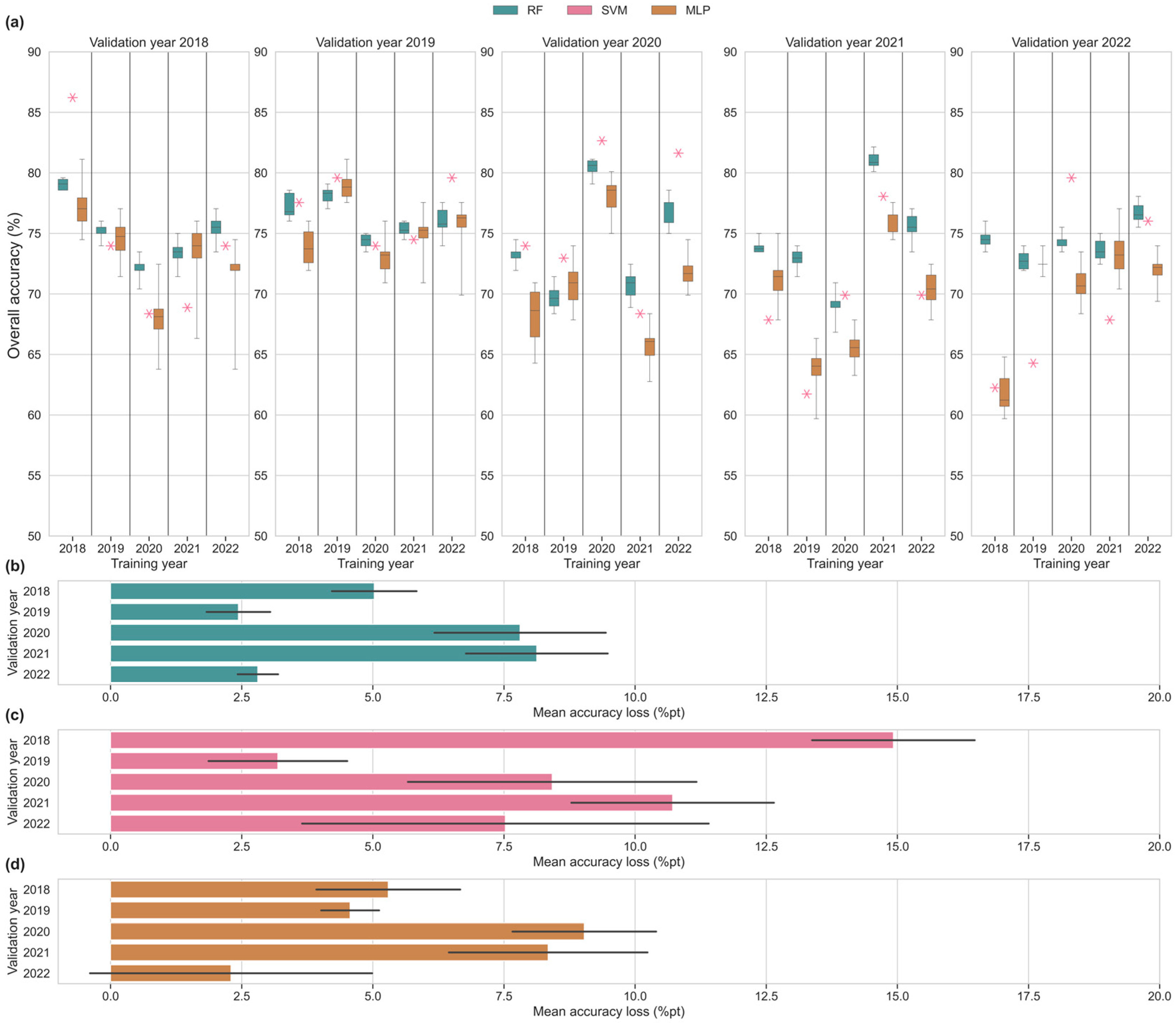
3.3. Cross-Year Single-Year Input Scenarios

For most validation years and algorithms, the baseline (same-year single-year) input scenarios consistently achieved a higher performance compared to the across-year single-year scenarios (Figure 7). A substantial drop in OA is usually observed when attempting temporal transferability. The average losses in OA are different for each year and each algorithm. They range from 2.81 ± 0.77%pt (2022) to 8.12 ± 2.71%pt (2021) for RF, from 3.19% ± 2.65 (2019) to 14.92% ± 3.10 (2018) for SVM, and from 2.30% ± 5.38 (2022) to 9.03% ± 2.74 for MLP.

These accuracy losses can be broken down into the specific losses in F1 score per individual class (

Table 4. Mean losses in F1 score (%pt) of Scots pine, black pine, oak, poplar, and beech and associated standard deviations per validation year for the cross-year single-year input scenarios compared to the same-year single-year input scenario of the same validation year for each applied classification algorithm: Random Forest (RF), Support Vector Machine (SVM), and Multilayer Perceptron (MLP).

		Validation Year
		2018	2019	2020	2021	2022
RF	Scots pine	4.47 ± 2.55	1.15 ± 1.01	2.16 ± 1.30	5.37 ± 1.66	−0.07 ± 1.63
	Black pine	−0.82 ± 5.99	4.24 ± 4.83	6.62 ± 3.96	9.82 ± 8.75	9.11 ± 4.19
	Oak	7.06 ± 5.24	−0.11 ± 4.49	11.84 ± 7.13	8.84 ± 6.59	6.97 ± 4.09
	Poplar	20.25 ± 24.68	8.57 ± 8.76	19.59 ± 15.95	25.85 ± 22.90	11.00 ± 10.49
	Beech	3.40 ± 4.48	7.64 ± 4.00	28.04 ± 12.43	11.29 ± 5.70	−1.17 ± 4.72
SVM	Scots pine	12.96 ± 2.97	−0.68 ± 2.22	3.53 ± 3.93	1.08 ± 6.2	5.15 ± 10.40
	Black pine	12.62 ± 5.25	6.12 ± 8.15	11.22 ± 6.71	10.20 ± 9.01	7.54 ± 5.03
	Oak	10.25 ± 10.44	−0.48 ± 12.10	14.43 ± 5.16	16.98 ± 10.27	5.90 ± 10.54
	Poplar	21.09 ± 6.80	20.52 ± 7.93	4.85 ± 5.55	39.22 ± 3.66	17.96 ± 12.51
	Beech	25.05 ± 11.38	11.86 ± 8.34	24.25 ± 18.68	31.43 ± 9.16	14.14 ± 8.84
MLP	Scots pine	1.57 ± 1.37	0.62 ± 0.87	3.04 ± 0.49	3.94 ± 4.08	−0.96 ± 4.92
	Black pine	0.09 ± 2.69	8.62 ± 7.04	8.00 ± 8.31	9.60 ± 12.01	−14.73 ± 3.62
	Oak	16.90 ± 14.81	10.34 ± 8.02	17.84 ± 6.30	17.41 ± 13.18	8.43 ± 5.20
	Poplar	28.57 ± 10.76	10.02 ± 3.82	21.36 ± 12.45	28.59 ± 16.65	20.14 ± 13.40
	Beech	7.51 ± 1.93	10.48 ± 2.96	34.12 ± 19.68	9.64 ± 2.71	11.57 ± 7.42

). The changes in accuracy exhibit large variations across species and validation years. The standard deviations are high due to the aggregation over the different input scenarios. In some cases, negative mean values indicate modest accuracy gains, but those are usually offset by large accuracy losses in other species.

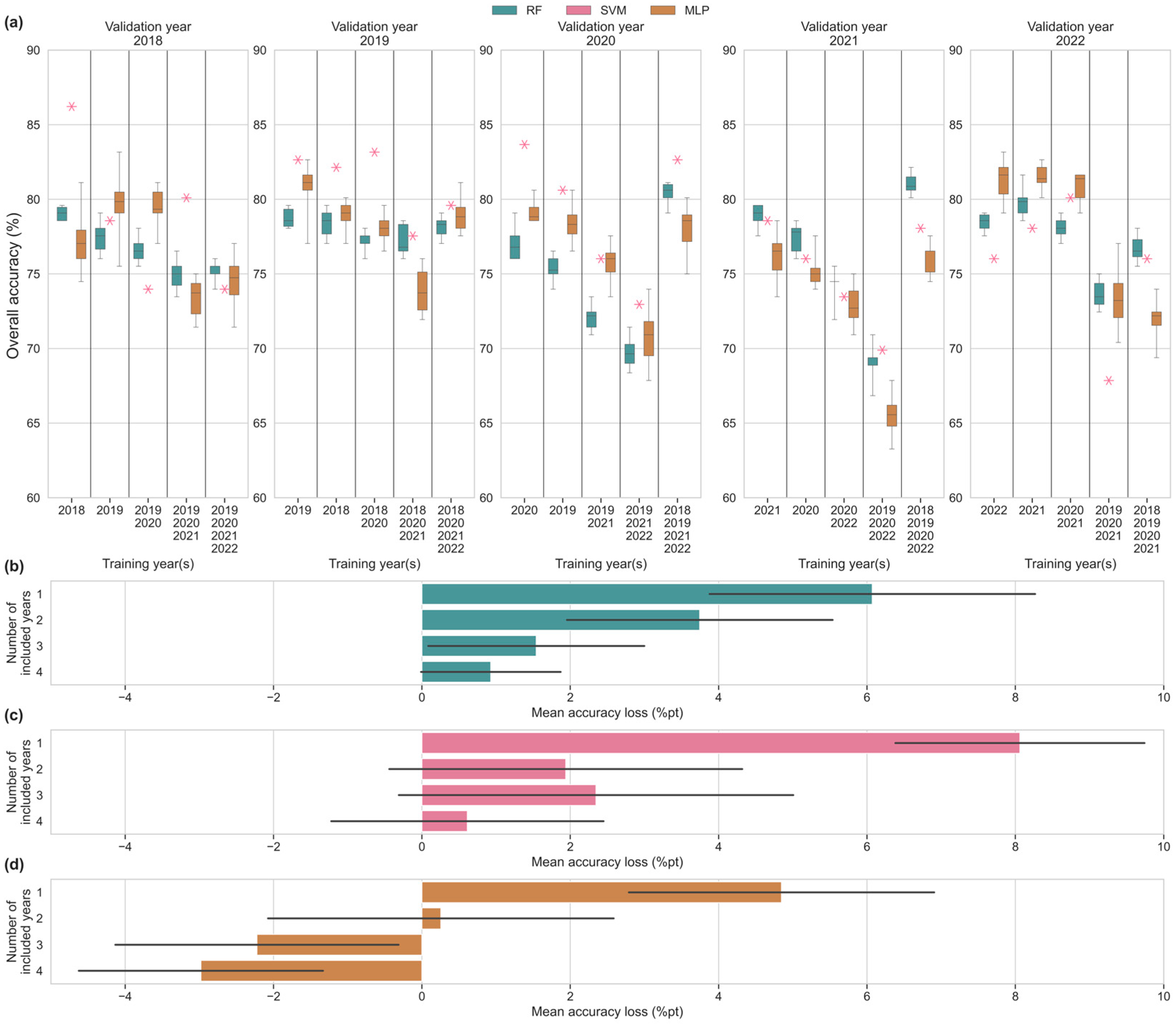
3.4. Multi-Year Input Scenarios

The multi-year input scenarios generally show improvements compared to the cross-year single-year scenarios (Figure 8). For RF, the mean loss in OA when one year was included in the training data was 6.07%pt ± 4.91. When two, three, or four years were included, this was reduced to 3.75%pt ± 4.00, 1.54%pt ± 3.26, and 0.93%pt ± 2.11, respectively. For SVM, the mean loss in OA when one year was included in the training data was 8.06%pt ± 3.76. When two, three, or four years were included, this was reduced to 1.94%pt ± 3.76, 2.35%pt ± 5.95, and 0.61%pt ± 4.10, respectively. For MLP, the mean loss in OA when one year was included in the training data was 4.85%pt ± 4.60. When two, three, or four years were included, this was reduced to 0.26%pt ± 5.21, −2.22%pt ± 4.27, and −2.98%pt ± 3.68, respectively. The aggregation over the different validation years results in high standard deviations, but nonetheless, the overall trend of reduced accuracy loss is apparent. For MLP, the use of multi-year training data sometimes even leads to modest improvements in OA compared to the same-year single-year scenario.

The F1 scores of the individual classes follow a similar pattern to the OA values, where the loss decreases or even becomes a gain as more training years are added (

Table 5. Mean losses in F1 score (%pt) of Scots pine, black pine, oak, poplar, and beech and associated standard deviations per number of included years for the multi-year input scenarios compared to the same-year single-year input scenario of the same validation year for each applied classification algorithm: Random Forest (RF), Support Vector Machine (SVM), and Multilayer Perceptron (MLP).

		Number of Years Included
		1	2	3	4
RF	Scots pine	2.97 ± 2.92	3.22 ± 3.50	2.33 ± 2.65	1.57 ± 2.16
	Black pine	7.99 ± 5.83	2.88 ± 3.74	−0.03 ± 4.07	−0.34 ± 2.59
	Oak	8.63 ± 7.60	4.99 ± 6.88	−2.03 ± 5.23	−1.87 ± 4.74
	Poplar	16.44 ± 17.52	3.74 ± 6.94	3.75 ± 4.46	1.90 ± 4.78
	Beech	9.61 ± 9.52	5.07 ± 11.17	1.00 ± 10.0	0.28 ± 8.31
SVM	Scots pine	3.12 ± 5.23	−1.07 ± 4.86	0.70 ± 6.97	−0.52 ± 5.07
	Black pine	8.35 ± 5.28	2.85 ± 3.12	3.23 ± 5.64	1.15 ± 3.32
	Oak	7.79 ± 12.35	3.89 ± 8.82	1.09 ± 7.67	−1.68 ± 5.34
	Poplar	23.72 ± 13.39	3.16 ± 4.74	5.34 ± 11.46	3.32 ± 7.41
	Beech	20.05 ± 11.29	12.01 ± 15.37	7.86 ± 10.17	6.79 ± 5.24
MLP	Scots pine	0.55 ± 3.12	−0.73 ± 3.04	−1.15 ± 2.31	−1.51 ± 1.80
	Black pine	−0.26 ± 11.73	−5.04 ± 12.99	−7.60 ± 11.88	−9.33 ± 9.71
	Oak	13.11 ± 10.28	4.80 ± 8.97	−3.00 ± 7.08	−4.81 ± 6.10
	Poplar	23.92 ± 13.63	1.69 ± 12.31	−4.28 ± 12.90	−5.46 ± 13.08
	Beech	14.19 ± 8.74	4.44 ± 14.44	−0.86 ± 9.86	−1.17 ± 9.80

). This is especially pronounced for the black pine, oak, poplar, and beech classes and less so for the Scots pine class.

4. Discussion

4.1. Baseline Model Performances

In previous studies, the reported overall accuracies are usually higher (>85%) than in our study when using RF or SVM [20,21,22,23,24,25,26,27,28,29,30]. Our lower overall model performance might have been caused by the smaller total size of the dataset, while our study area is relatively large and heterogeneous. However, our accuracies are generally still at an acceptable level (>75%). The OA values were mainly driven by the majority class, Scots pine, with F1 scores up to 89%. However, in other studies, the F1 scores for the majority classes were usually higher than 90%, contributing to a higher OA value. Indeed, it is common that the predictive probability distribution of the classification model is skewed towards the majority class [72,73]. Furthermore, our main goal was to investigate and quantify temporal transferability by assessing and comparing model performances of same-year and cross-year scenarios. To do this, comparable (i.e., containing comparable spectral information in predefined time ranges) time series were constructed for the different years. We thus opted to not include a feature selection step, which might have improved the performances of individual models by reducing the dimensionality of the dataset, as this was not the main focus of this study. On the other hand, other studies also experienced a large variation in individual class accuracies. Compared to the more common tree species, less widespread tree species are usually affected by a high rate of classification errors due to small sample sizes and partial overlap in spectral signatures [25,27]. In our case, reasonably high accuracies were achieved for oak (>79%) with all three methods. SVM also consistently achieved reasonably high accuracies for Beech (>70%), while RF and SVM did so for poplar (>70%).

Out of the three algorithms that were tested, RF and SVM showed superior performance for the single-year same-year input scenarios compared to MLP. The performance of MLP was less robust within one input scenario as well as across different validation years. This makes the method less reliable than RF and SVM, which could explain the popularity of the latter two methods. This corresponds to the findings of Zagajewski et al. [31], who also compared RF, SVM, and MLP and concluded that RF and SVM were the preferred methods over MLP. Our comparison between RF and SVM yielded a less straightforward outcome. On the one hand, SVM performed better in three out of five evaluated years. This corresponds to other studies in which SVM outperformed RF [22,23,31]. On the other hand, the performance of SVM varied more across the different years. It is therefore difficult to say that one method is unequivocally better than the other and to subsequently recommend one above the other. Surprisingly, this is also in line with the recommendations from the aforementioned studies which suggest that RF and SVM both remain suitable for this application [22,23,31].

4.2. Assessment of Temporal Transferability

Our results showed that the same-year baseline models usually performed better compared to their cross-year counterparts. This confirms that the relationships between the spectral data and target classes are not necessarily consistent in time, also in the context of tree species classification. Each evaluated method suffered from a loss in OA, although the size of the decrease varied considerably for different validation years. In general, the models were still able to classify Scots pine with an acceptable level of accuracy across years. However, that cannot be said for the other tree species, especially poplar, which was consistently classified with a much lower accuracy. For black pine, oak, and beech, the performance loss varied considerably for the different years. It is, however, difficult to attribute these differences to a specific cause. Even so, it is likely that interannual differences in climate and image quality play a role, as also suggested by Kyere et al. [37]. In Belgium, heat waves occurred in July 2018, July 2019, August 2020, and August 2022. These years were also relatively dry. Conversely, 2021 was a very wet year with slightly cooler temperatures than usual. In July 2021, an extreme precipitation event resulted in severe floods. It is not straightforward to link these events to the NDVI curves of Figure 5. However, it can be seen that the 2021 curves deviated most from the other years from January until June. It is possible that this was caused by the increased wetness after three hot and dry years, which could affect the spectra.

To the best of our knowledge, there are no similar studies in the field of tree species classification using satellite imagery with which to compare our findings. However, similar decreases in classification performance have been observed in studies that focus on land cover classification or crop type classification. For example, in the context of corn and soybean mapping with Landsat imagery, Zhong et al. [74] found a similar decrease in RF classification performance. The average same-year accuracy was 90.1%, while the average cross-year accuracy was 75.5%. Another example is Gray et al. [35], in which an accuracy drop of approximately 10%pt was found for land cover classification with RF.

The standard deviations of our results are large because they are aggregated over different training years. This indicates that decreases in (individual class) accuracy range between modest and severe. Sometimes temporal transfers lead to modest improvements in individual class accuracies, while other times it lead to severe deterioration of individual class accuracies. This underlines the unpredictability of temporal transferability. More research is needed to better understand this phenomenon.

4.3. Impact Multi-Year Training Data

Our results indicate that the use of multi-year training data can reduce the drop in classification performance, and thereby improve the temporal generalisation ability of a trained classification model. For each evaluated method, an incremental positive effect was observed when up to four years were added. Compared to the same-year single-year approach, this strategy even led to gains in OA and F1 scores in some cases, most notably for MLP. MLP thus benefitted most from additional training data from different years. This suggests that MLP is able to utilise the additional data in a more effective way.

In general, our methods are applicable to other regions with other species compositions. We employed a clear preprocessing workflow for the satellite data that can be applied to any region as long as the level of cloud cover is not too excessive. The obtained time series consist of aggregated observations at predetermined intervals, eliminating the reliance on satellite data on specific dates. Moreover, the experimental set-up of this study can be replicated with other tree species classes or even labels from applications outside of tree species classification.

The current study was limited to five years of Sentinel-2 data; it is unclear whether the full potential of this improvement has been achieved. Future studies could build on these experimental findings and expand the temporal range, thereby including more climatic and environmental variations. However, there is most likely a limit to expanding the temporal range given that forests will at some point change too much for labels to remain valid. In this case, data augmentation techniques for time series could be useful. Data augmentation techniques have recently been receiving more attention as a promising route to alleviate limitations in data quantity, for instance for image target recognition [75], or when using deep learning [76]. Data augmentation techniques that work for time series that are used in other disciplines could also offer interesting research opportunities [77,78].

Alternatively, it would be useful to explore other strategies to improve temporal transferability. The general idea would be to better capture the temporal dynamics and include them in the input feature space. One possibility could be the incorporation of meteorological variables and phenological metrics as classification inputs to capture inter-annual variations in phenology. For example, Zhong et al. [74] found that the use of phenological metrics as inputs improved the temporal extendibility of an RF classifier. Another possibility could lie in the use of algorithms that can take into account the temporal ordering of the input features. In this respect, neural network-based methods could be promising. For instance, Gray et al. [35] found recurrent convolutional networks to be useful in a context where temporal transferability was important. However, such networks typically require large datasets for model training, which are generally not available in most remote sensing applications. Again, a promising path to mitigate this issue could be data augmentation.

4.4. Data Limitations

In this study, the existing data record of one full inventory cycle of RFI of Flanders was leveraged to investigate dominant tree species classification across different years. However, it should be acknowledged that these data, similar to other forest inventories, were not gathered specially for the purpose of developing remote sensing-based classification models [79]. Consequently, this dataset does not completely align with the ideal criteria described in Fassnacht et al. [6]. Even though the full inventory is representative of the whole area of Flanders, a plot selection procedure was necessary to create a suitable dataset for this application. In short, the subset is not fully representative of the variation that is actually present in the study area. First, only plots with certain characteristics were selected from the entire RFI dataset (see Section 2.2.1), reducing the data variability compared to what is present in reality. Second, given how the dominant tree species labels were defined, a selection of sufficiently homogeneous plots was made. This is customary in this type of studies because mixed plots represent mixed forests which have a larger spectral variation and are thus more difficult to classify correctly. Third, only five tree species were considered in this study. Although these target classes are very relevant to the study area, other forest tree species occur in Flanders. The other species can also be important in terms of ecological or economic value. However, the accurate classification of less common tree species remains a challenge, since it is difficult to obtain a large amount of reference samples that capture the entire within-class variation. Finally, even though no specific selection was made, it is unlikely that the subset of the RFI data included all possible development stages and age classes of the target classes.

5. Conclusions

This study reaffirms the potential of multitemporal Sentinel-2 data for temperate forest tree species classification. In a standard single-year setting, classification performances of 75% and higher were achieved with the RF and SVM algorithms. The effect of temporally transferring trained models was thoroughly investigated through a comparison of so-called input scenarios. A mean decrease in overall accuracy between 2.30 and 14.92 percentage points was observed for different years and different algorithms. This can hinder the operational application of trained classification models. However, our results suggest that the use of multi-year training data can reduce this drop in overall accuracy as satellite data from different years is added. Therefore, we recommend incorporating interannual variability into the training stage of tree species classification models to maximise their temporal transferability to unseen years.

References

1. Brockerhoff, E.G.; Barbaro, L.; Castagneyrol, B.; Forrester, D.I.; Gardiner, B.; González-Olabarria, J.R.; Lyver, P.O.B.; Meurisse, N.; Oxbrough, A.; Taki, H.; et al. Forest Biodiversity, Ecosystem Functioning and the Provision of Ecosystem Services. Biodivers. Conserv. 2017, 26, 3005–3035. [Google Scholar] [CrossRef]
2. Gamfeldt, L.; Snäll, T.; Bagchi, R.; Jonsson, M.; Gustafsson, L.; Kjellander, P.; Ruiz-Jaen, M.C.; Fröberg, M.; Stendahl, J.; Philipson, C.D.; et al. Higher Levels of Multiple Ecosystem Services Are Found in Forests with More Tree Species. Nat. Commun. 2013, 4, 1340. [Google Scholar] [CrossRef] [PubMed]
3. Rogers, P.C. Disturbance Ecology; Wohlgemuth, T., Jentsch, A., Seidl, R., Eds.; Landscape Series; Springer: Cham, Switzerland, 2022; Volume 32, ISBN 978-3-030-98755-8. [Google Scholar]
4. Boisvenue, C.; White, J. Information Needs of Next-Generation Forest Carbon Models: Opportunities for Remote Sensing Science. Remote Sens. 2019, 11, 463. [Google Scholar] [CrossRef]
5. Shaw, C.H.; Bona, K.A.; Kurz, W.A.; Fyles, J.W. The Importance of Tree Species and Soil Taxonomy to Modeling Forest Soil Carbon Stocks in Canada. Geoderma Reg. 2015, 4, 114–125. [Google Scholar] [CrossRef]
6. Fassnacht, F.E.; Latifi, H.; Stereńczak, K.; Modzelewska, A.; Lefsky, M.; Waser, L.T.; Straub, C.; Ghosh, A. Review of Studies on Tree Species Classification from Remotely Sensed Data. Remote Sens. Environ. 2016, 186, 64–87. [Google Scholar] [CrossRef]
7. Pu, R. Mapping Tree Species Using Advanced Remote Sensing Technologies: A State-of-the-Art Review and Perspective. J. Remote Sens. 2021, 2021, 9812624. [Google Scholar] [CrossRef]
8. Immitzer, M.; Atzberger, C.; Koukal, T. Tree Species Classification with Random Forest Using Very High Spatial Resolution 8-Band WorldView-2 Satellite Data. Remote Sens. 2012, 4, 2661–2693. [Google Scholar] [CrossRef]
9. Ballanti, L.; Blesius, L.; Hines, E.; Kruse, B. Tree Species Classification Using Hyperspectral Imagery: A Comparison of Two Classifiers. Remote Sens. 2016, 8, 445. [Google Scholar] [CrossRef]
10. Dalponte, M.; Orka, H.O.; Gobakken, T.; Gianelle, D.; Naesset, E. Tree Species Classification in Boreal Forests with Hyperspectral Data. IEEE Trans. Geosci. Remote Sens. 2013, 51, 2632–2645. [Google Scholar] [CrossRef]
11. Michałowska, M.; Rapiński, J. A Review of Tree Species Classification Based on Airborne LiDAR Data and Applied Classifiers. Remote Sens. 2021, 13, 353. [Google Scholar] [CrossRef]
12. White, J.C.; Coops, N.C.; Wulder, M.A.; Vastaranta, M.; Hilker, T.; Tompalski, P. Remote Sensing Technologies for Enhancing Forest Inventories: A Review. Can. J. Remote Sens. 2016, 42, 619–641. [Google Scholar] [CrossRef]
13. Ørka, H.O.; Hauglin, M. Use of Remote Sensing for Mapping of Non-Native Conifer Species. Ina Fagrapp. 2016, 33, 1–76. [Google Scholar]
14. Woodcock, C.E.; Allen, R.; Anderson, M.; Belward, A.; Bindschadler, R.; Cohen, W.; Gao, F.; Goward, S.N.; Helder, D.; Helmer, E.; et al. Free Access to Landsat Imagery. Science 2008, 320, 1011. [Google Scholar] [CrossRef] [PubMed]
15. Aschbacher, J.; Milagro-Pérez, M.P. The European Earth Monitoring (GMES) Programme: Status and Perspectives. Remote Sens. Environ. 2012, 120, 3–8. [Google Scholar] [CrossRef]
16. Immitzer, M.; Vuolo, F.; Atzberger, C. First Experience with Sentinel-2 Data for Crop and Tree Species Classifications in Central Europe. Remote Sens. 2016, 8, 166. [Google Scholar] [CrossRef]
17. Fassnacht, F.E.; Neumann, C.; Forster, M.; Buddenbaum, H.; Ghosh, A.; Clasen, A.; Joshi, P.K.; Koch, B. Comparison of Feature Reduction Algorithms for Classifying Tree Species with Hyperspectral Data on Three Central European Test Sites. IEEE J. Sel. Top. Appl. Earth Obs. Remote Sens. 2014, 7, 2547–2561. [Google Scholar] [CrossRef]
18. Dalponte, M.; Bruzzone, L.; Gianelle, D. Tree Species Classification in the Southern Alps Based on the Fusion of Very High Geometrical Resolution Multispectral/Hyperspectral Images and LiDAR Data. Remote Sens. Environ. 2012, 123, 258–270. [Google Scholar] [CrossRef]
19. Heikkinen, V.; Tokola, T.; Parkkinen, J.; Korpela, I.; Jaaskelainen, T. Simulated Multispectral Imagery for Tree Species Classification Using Support Vector Machines. IEEE Trans. Geosci. Remote Sens. 2010, 48, 1355–1364. [Google Scholar] [CrossRef]
20. Bolyn, C.; Michez, A.; Gaucher, P.; Lejeune, P.; Bonnet, S. Forest Mapping and Species Composition Using Supervised per Pixel Classification of Sentinel-2 Imagery. BASE 2018, 22, 172–187. [Google Scholar] [CrossRef]
21. Breidenbach, J.; Waser, L.T.; Debella-Gilo, M.; Schumacher, J.; Rahlf, J.; Hauglin, M.; Puliti, S.; Astrup, R. National Mapping and Estimation of Forest Area by Dominant Tree Species Using Sentinel-2 Data. Can. J. For. Res. 2021, 51, 365–379. [Google Scholar] [CrossRef]
22. Wessel, M.; Brandmeier, M.; Tiede, D. Evaluation of Different Machine Learning Algorithms for Scalable Classification of Tree Types and Tree Species Based on Sentinel-2 Data. Remote Sens. 2018, 10, 1419. [Google Scholar] [CrossRef]
23. Grabska, E.; Frantz, D.; Ostapowicz, K. Evaluation of Machine Learning Algorithms for Forest Stand Species Mapping Using Sentinel-2 Imagery and Environmental Data in the Polish Carpathians. Remote Sens. Environ. 2020, 251, 112103. [Google Scholar] [CrossRef]
24. Hemmerling, J.; Pflugmacher, D.; Hostert, P. Mapping Temperate Forest Tree Species Using Dense Sentinel-2 Time Series. Remote Sens. Environ. 2021, 267, 112743. [Google Scholar] [CrossRef]
25. Grabska, E.; Hostert, P.; Pflugmacher, D.; Ostapowicz, K. Forest Stand Species Mapping Using the Sentinel-2 Time Series. Remote Sens. 2019, 11, 1197. [Google Scholar] [CrossRef]
26. Hościło, A.; Lewandowska, A. Mapping Forest Type and Tree Species on a Regional Scale Using Multi-Temporal Sentinel-2 Data. Remote Sens. 2019, 11, 929. [Google Scholar] [CrossRef]
27. Immitzer, M.; Neuwirth, M.; Böck, S.; Brenner, H.; Vuolo, F.; Atzberger, C. Optimal Input Features for Tree Species Classification in Central Europe Based on Multi-Temporal Sentinel-2 Data. Remote Sens. 2019, 11, 2599. [Google Scholar] [CrossRef]
28. Karasiak, N.; Fauvel, M.; Dejoux, J.-F.; Monteil, C.; Sheeren, D. Optimal dates for deciduous tree species mapping using full years Sentinel-2 time series in south west France. ISPRS Ann. Photogramm. Remote Sens. Spat. Inf. Sci. 2020, 3, 469–476. [Google Scholar] [CrossRef]
29. Persson, M.; Lindberg, E.; Reese, H. Tree Species Classification with Multi-Temporal Sentinel-2 Data. Remote Sens. 2018, 10, 1794. [Google Scholar] [CrossRef]
30. Kollert, A.; Bremer, M.; Löw, M.; Rutzinger, M. Exploring the Potential of Land Surface Phenology and Seasonal Cloud Free Composites of One Year of Sentinel-2 Imagery for Tree Species Mapping in a Mountainous Region. Int. J. Appl. Earth Obs. Geoinf. 2021, 94, 102208. [Google Scholar] [CrossRef]
31. Zagajewski, B.; Kluczek, M.; Raczko, E.; Njegovec, A.; Dabija, A.; Kycko, M. Comparison of Random Forest, Support Vector Machines, and Neural Networks for Post-Disaster Forest Species Mapping of the Krkonoše/Karkonosze Transboundary Biosphere Reserve. Remote Sens. 2021, 13, 2581. [Google Scholar] [CrossRef]
32. Grabska-Szwagrzyk, E.; Tymińska-Czabańska, L. Sentinel-2 Time Series: A Promising Tool in Monitoring Temperate Species Spring Phenology. For. An Int. J. For. Res. 2023, 97, 267–281. [Google Scholar] [CrossRef]
33. Hill, R.A.; Wilson, A.K.; George, M.; Hinsley, S.A. Mapping Tree Species in Temperate Deciduous Woodland Using Time-Series Multi-Spectral Data. Appl. Veg. Sci. 2010, 13, 86–99. [Google Scholar] [CrossRef]
34. Sheeren, D.; Fauvel, M.; Josipovíc, V.; Lopes, M.; Planque, C.; Willm, J.; Dejoux, J.F. Tree Species Classification in Temperate Forests Using Formosat-2 Satellite Image Time Series. Remote Sens. 2016, 8, 734. [Google Scholar] [CrossRef]
35. Gray, P.C.; Chamorro, D.F.; Ridge, J.T.; Kerner, H.R.; Ury, E.A.; Johnston, D.W. Temporally Generalizable Land Cover Classification: A Recurrent Convolutional Neural Network Unveils Major Coastal Change through Time. Remote Sens. 2021, 13, 3953. [Google Scholar] [CrossRef]
36. Wijesingha, J.; Dzene, I.; Wachendorf, M. Evaluating the Spatial–Temporal Transferability of Models for Agricultural Land Cover Mapping Using Landsat Archive. ISPRS J. Photogramm. Remote Sens. 2024, 213, 72–86. [Google Scholar] [CrossRef]
37. Kyere, I.; Astor, T.; Graß, R.; Wachendorf, M. Multi-Temporal Agricultural Land-Cover Mapping Using Single-Year and Multi-Year Models Based on Landsat Imagery and IACS Data. Agronomy 2019, 9, 309. [Google Scholar] [CrossRef]
38. Momm, H.G.; ElKadiri, R.; Porter, W. Crop-Type Classification for Long-Term Modeling: An Integrated Remote Sensing and Machine Learning Approach. Remote Sens. 2020, 12, 449. [Google Scholar] [CrossRef]
39. Jin, S.; Su, Y.; Gao, S.; Hu, T.; Liu, J.; Guo, Q. The Transferability of Random Forest in Canopy Height Estimation from Multi-Source Remote Sensing Data. Remote Sens. 2018, 10, 1183. [Google Scholar] [CrossRef]
40. Domingo, D.; Alonso, R.; Lamelas, M.T.; Montealegre, A.L.; Rodríguez, F.; de la Riva, J. Temporal Transferability of Pine Forest Attributes Modeling Using Low-Density Airborne Laser Scanning Data. Remote Sens. 2019, 11, 261. [Google Scholar] [CrossRef]
41. Fekety, P.A.; Falkowski, M.J.; Hudak, A.T. Temporal Transferability of LiDAR-Based Imputation of Forest Inventory Attributes. Can. J. For. Res. 2015, 45, 422–435. [Google Scholar] [CrossRef]
42. de Lera Garrido, A.; Gobakken, T.; Ørka, H.O.; Næsset, E.; Bollandsås, O.M. Reuse of Field Data in Als-Assisted Forest Inventory. Silva Fenn. 2020, 54, 10272. [Google Scholar] [CrossRef]
43. Tuia, D.; Persello, C.; Bruzzone, L. Domain Adaptation for the Classification of Remote Sensing Data: An Overview of Recent Advances. IEEE Geosci. Remote Sens. Mag. 2016, 4, 41–57. [Google Scholar] [CrossRef]
44. Estrella, N.; Menzel, A. Responses of Leaf Colouring in Four Deciduous Tree Species to Climate and Weather in Germany. Clim. Res. 2006, 32, 253–267. [Google Scholar] [CrossRef]
45. Xie, Y.; Wang, X.; Wilson, A.M.; Silander, J.A. Predicting Autumn Phenology: How Deciduous Tree Species Respond to Weather Stressors. Agric. For. Meteorol. 2018, 250–251, 127–137. [Google Scholar] [CrossRef]
46. Meier, M.; Vitasse, Y.; Bugmann, H.; Bigler, C. Phenological Shifts Induced by Climate Change Amplify Drought for Broad-Leaved Trees at Low Elevations in Switzerland. Agric. For. Meteorol. 2021, 307, 108485. [Google Scholar] [CrossRef]
47. Duan, S.; He, H.S.; Spetich, M. Effects of Growing-Season Drought on Phenology and Productivity in Thewest Region of Central Hardwood Forests, USA. Forests 2018, 9, 377. [Google Scholar] [CrossRef]
48. Xie, Y.; Wang, X.; Silander, J.A. Deciduous Forest Responses to Temperature, Precipitation, and Drought Imply Complex Climate Change Impacts. Proc. Natl. Acad. Sci. USA 2015, 112, 13585–13590. [Google Scholar] [CrossRef]
49. Govaere, L.; Leyman, A. Vlaamse Bosinventarisatie Agentschap Natuur En Bos (VBI1: 1997-1999; VBI2: 2009–2018; VBI3: 2019–2021). Available online: https://www.natuurenbos.be/vlaamse-bosinventaris/Website_BosAreaal.html (accessed on 8 December 2023).
50. Forest Europe. State of Europe’s Forests 2020; Forest Europe: Bonn, Germany, 2020. [Google Scholar]
51. Schneiders, A.; Alaerts, K.; Michels, H.; Stevens, M.; Van Gossum, P.; Van Reeth, W.; Vught, I. Natuurrapport 2020: Feiten En Cijfers Voor Een Nieuw Biodiversiteitsbeleid; Research Institute Nature and Forest: Brussels, Belgium, 2020. [Google Scholar]
52. Vandekerkhove, K. Integration of Nature Protection in Forest Policy in Flanders (Belgium); European Forest Institute: Freiburg, Germany, 2013. [Google Scholar]
53. Govaere, L. Een Blik Op de Kenmerken van Bos in Vlaanderen–Eerste Resultaten van Twee Opeenvolgende Vlaamse Bosinventarisaties. Bosrevue 2020, 83, 1–14. [Google Scholar]
54. Zanaga, D.; Van De Kerchove, R.; Daems, D.; De Keersmaecker, W.; Brockmann, C.; Kirches, G.; Wevers, J.; Cartus, O.; Santoro, M.; Fritz, S.; et al. ESA WorldCover 10 m 2021 V200 2022; Zenodo: Geneva, Switzerland. [CrossRef]
55. ANF Bosinventaris. Available online: https://www.natuurenbos.be/beleid-wetgeving/natuurbeheer/bosinventaris (accessed on 13 November 2023).
56. Govaere, L.; Van de Kerckhove, P.; Roelandt, B.; Sannen, P.; Schrey, L. Handleiding Tweede Bosinventarisatie Vlaams Gewest; Agency for Nature and Forests: Brussels, Belgium, 2009. [Google Scholar]
57. Govaere, L. Protocol En Handleiding Derde Bosinventarisatie Vlaams Gewest; Agency for Nature and Forests: Brussels, Belgium, 2019. [Google Scholar]
58. Dumortier, M.; Van Gossum, P.; Van Calster, H.; Adriaens, D.; Adriaenssens, V.; Alaerts, K.; Brys, R.; Cools, N.; De Knijf, G.; Denys, L.; et al. Voorstel Voor Een Meetnet Biodiversiteit Agrarisch Gebied; Nr. INBO.A.4387; Adviezen van Het Instituut Voor Natuur-En Bosonderzoek; Research Institute Nature and Forest: Brussels, Belgium, 2022; pp. 1–51. [Google Scholar]
59. Schramm, M.; Pebesma, E.; Milenković, M.; Foresta, L.; Dries, J.; Jacob, A.; Wagner, W.; Mohr, M.; Neteler, M.; Kadunc, M.; et al. The Openeo Api–Harmonising the Use of Earth Observation Cloud Services Using Virtual Data Cube Functionalities. Remote Sens. 2021, 13, 1125. [Google Scholar] [CrossRef]
60. Dries, J.; Lippens, S. openeo-python-client (Version 0.22.0). Available online: https://github.com/Open-EO/openeo-python-client (accessed on 15 July 2024).
61. Terrascope Terrascope. Available online: https://terrascope.be/en (accessed on 14 September 2023).
62. Swinnen, E.; De Keukelaere, L. Terrascope Sentinel-2-Quality Assessment Report; Flemish Institute for Technological Research (VITO): Mol, Belgium, 2020; pp. 1–42. [Google Scholar]
63. Richter, R.; Louis, J.; Müller-Wilm, U. Sentinel-2 MSI–Level 2A Products Algorithm Theoretical Basis Document; S2PAD-ATBD-0001, Issue 2.0; Telespazio VEGA Deutschland GmbH: Darmstadt, Germany, 2012. [Google Scholar]
64. Tucker, C.J. Red and Photographic Infrared Linear Combinations for Monitoring Vegetation. Remote Sens. Environ. 1979, 8, 127–150. [Google Scholar] [CrossRef]
65. Hermosilla, T.; Bastyr, A.; Coops, N.C.; White, J.C.; Wulder, M.A. Mapping the Presence and Distribution of Tree Species in Canada’s Forested Ecosystems. Remote Sens. Environ. 2022, 282, 113276. [Google Scholar] [CrossRef]
66. Stas, M.; Van Orshoven, J.; Dong, Q.; Heremans, S.; Zhang, B. A Comparison of Machine Learning Algorithms for Regional Wheat Yield Prediction Using NDVI Time Series of SPOT-VGT. In Proceedings of the 2016 Fifth International Conference on Agro-Geoinformatics (Agro-Geoinformatics), Tianjin, China, 18–20 July 2016; IEEE: Piscartway, NJ, USA, 2016; pp. 1–5. [Google Scholar] [CrossRef]
67. Savitzky, A.; Golay, M.J.E. Smoothing and Differentiation of Data by Simplified Least Squares Procedures. Anal. Chem. 1964, 36, 1627–1639. [Google Scholar] [CrossRef]
68. Breiman, L. Random Forests. Mach. Learn. 2001, 45, 5–32. [Google Scholar] [CrossRef]
69. Mountrakis, G.; Im, J.; Ogole, C. Support Vector Machines in Remote Sensing: A Review. ISPRS J. Photogramm. Remote Sens. 2011, 66, 247–259. [Google Scholar] [CrossRef]
70. Wang, Z.; Yan, W.; Oates, T. Time Series Classification from Scratch with Deep Neural Networks: A Strong Baseline. In Proceedings of the 2017 International Joint Conference on Neural Networks (IJCNN), Anchorage, AK, USA, 4–9 June 2017; IEEE: Piscartway, NJ, USA, 2017; Volume 2017-May, pp. 1578–1585. [Google Scholar] [CrossRef]
71. Zhong, L.; Hu, L.; Zhou, H. Deep Learning Based Multi-Temporal Crop Classification. Remote Sens. Environ. 2019, 221, 430–443. [Google Scholar] [CrossRef]
72. Akbani, R.; Kwek, S.; Japkowicz, N. Applying Support Vector Machines to Imbalanced Datasets. In European Conference on Machine Learning; Springer: Berlin/Heidelberg, Germany, 2004; pp. 39–50. [Google Scholar] [CrossRef]
73. Chen, C.; Liaw, A.; Breiman, L. Using Random Forest to Learn Imbalanced Data; Department of Statistics, University of California: Berkeley, CA, USA, 2004. [Google Scholar]
74. Zhong, L.; Gong, P.; Biging, G.S. Efficient Corn and Soybean Mapping with Temporal Extendability: A Multi-Year Experiment Using Landsat Imagery. Remote Sens. Environ. 2014, 140, 1–13. [Google Scholar] [CrossRef]
75. Hao, X.; Liu, L.; Yang, R.; Yin, L.; Zhang, L.; Li, X. A Review of Data Augmentation Methods of Remote Sensing Image Target Recognition. Remote Sens. 2023, 15, 827. [Google Scholar] [CrossRef]
76. Yang, S.; Xiao, W.; Zhang, M.; Guo, S.; Zhao, J.; Shen, F. Image Data Augmentation for Deep Learning: A Survey. arXiv 2022, arXiv:2204.08610. [Google Scholar]
77. Iwana, B.K.; Uchida, S. An Empirical Survey of Data Augmentation for Time Series Classification with Neural Networks. PLoS ONE 2021, 16, e0254841. [Google Scholar] [CrossRef]
78. Iglesias, G.; Talavera, E.; González-Prieto, Á.; Mozo, A.; Gómez-Canaval, S. Data Augmentation Techniques in Time Series Domain: A Survey and Taxonomy. Neural Comput. Appl. 2023, 35, 10123–10145. [Google Scholar] [CrossRef]
79. Westra, T.; Verschelde, P.; Van Calster, H.; Lommelen, E.; Onkelinx, T.; Quataert, P.; Govaere, L. Opmaak van Een Analysestramien Voor de Gegevens van de Vlaamse Bosinventarisatie. Rapporten van het Instituu voor Natuur- en Bosonderzoek 2015; Research Institute for Nature and Forest: Brussels, Belgium, 2015. [Google Scholar]
Figure 1. Visual representation of the applied workflow divided into three components: data sources, data preparation, and model training and evaluation.
Remotesensing 16 02653 g001
Figure 2. Localisation of the study area (left) and map of Flanders with forested area according to the ESA WorldCover 10 m 2021 v200 product (right) [54].
Remotesensing 16 02653 g002
Figure 3. Localisation of the 653 plots of the Regional Forest Inventory of Flanders used in this study. Each colour represents one of the five dominant tree species target classes.
Remotesensing 16 02653 g003
Figure 4. Overview of the three groups of applied classification approaches: (a) the same-year single-year input scenarios, (b) the cross-year single-year input scenarios, and (c) the cross-year multi-year input scenarios.
Remotesensing 16 02653 g004
Figure 5. Species-specific mean NDVI curves for each examined year (2018, 2019, 2020, 2021, and 2022) for (a) Scots pine, (b) black pine, (c) oak, (d) poplar, and (e) beech.
Remotesensing 16 02653 g005
Figure 6. Overall accuracies (OA, %) of the same-year single-year input scenarios for each tested classification algorithm: Random Forest (RF), Support Vector Machine (SVM), and Multilayer Perceptron (MLP). For RF and MLP, each boxplot represents the range of OA values for the 10 executed repetitions of model training and validation. For SVM, each asterisk represents the resulting OA value, since there is no variance due to random initialization.
Remotesensing 16 02653 g006
Figure 7. (a) Overall accuracies (OA) (%) for the cross-year single-year input scenarios for the three tested algorithms: Random Forest (RF), Support Vector Machine (SVM), and Multilayer Perceptron (MLP). For RF and MLP, each boxplot represents the range of OA values for the 10 executed repetitions of model training and validation. For SVM, each asterisk represents the resulting OA value, since there is no variance due to random initialization. For reference, the same-year single-year classifications are added. (bd) Mean accuracy loss (%pt) per validation year with standard error bars for the cross-year single-year input scenarios compared to the same-year single-year input scenario of the same validation year for (b) RF, (c) SVM, and (d) MLP.
Remotesensing 16 02653 g007
Figure 8. (a) Overall accuracies (OA) (%) for the multi-year input scenarios for the three tested algorithms: Random Forest (RF), Support Vector Machine (SVM), and Multilayer Perceptron (MLP). For RF and MLP, each boxplot represents the range of OA values for the 10 executed repetitions of model training and validation. For SVM, each asterisk represents the resulting OA value, since there is no variance due to random initialization. The same-year single-year classifications are added as baseline reference, along with one of the cross-year single-year scenarios. (bd) Mean accuracy loss (%pt) per number of included training years with standard error bars for the multi-year input scenarios compared to the same-year single-year input scenario of the corresponding validation year for (b) RF, (c) SVM, and (d) MLP.
Remotesensing 16 02653 g008