Contrasting the Effects of X-Band Phased Array Radar and S-Band Doppler Radar Data Assimilation on Rainstorm Forecasting in the Pearl River Delta

Abstract

Contrasting the X-band phased array radar (XPAR) with the conventional S-Band dual-polarization mechanical scanning radar (SMSR), the XPAR offers superior temporal and spatial resolution, enabling a more refined depiction of the internal dynamics within convective systems. While both SMSR and XPAR data are extensively used in monitoring and alerting for severe convective weather, their comparative application in numerical weather prediction through data assimilation remains a relatively unexplored area. This study harnesses the Weather Research and Forecasting Model (WRF) and its data assimilation system (WRFDA) to integrate radial velocity and reflectivity from the Guangzhou SMSR and nine XPARs across Guangdong Province. Utilizing a three-dimensional variational approach at a 1 km convective-scale grid, the assimilated data are applied to forecast a rainstorm event in the Pearl River Delta (PRD) on 6 June 2022. Through a comparative analysis of the results from assimilating SMSR and XPAR data, it was observed that the assimilation of SMSR data led to more extensive adjustments in the lower- and middle-level wind fields compared to XPAR data assimilation. This resulted in an enlarged convergence area at lower levels, prompting an overdevelopment of convective systems and an excessive concentration of internal hydrometeor particles, which in turn led to spurious precipitation forecasts. However, the sequential assimilation of both SMSR and XPAR data effectively reduced the excessive adjustments in the wind fields that were evident when only SMSR data were used. This approach diminished the generation of false echoes and enhanced the precision of quantitative precipitation forecasts. Additionally, the lower spectral width of XPAR data indicates its superior detection accuracy. Assimilating XPAR data alone yields more reasonable adjustments to the low- to middle-level wind fields, leading to the formation of small-to-medium-scale horizontal convergence lines in the lower levels of the analysis field. This enhancement significantly improves the model’s forecasts of composite reflectivity and radar echoes, aligning them more closely with actual observations. Consequently, the Threat Score (TS) and Equitable Threat Score (ETS) for heavy-rain forecasts (>10 mm/h) over the next 5 h are markedly enhanced. This study underscores the necessity of incorporating XPAR data assimilation in numerical weather prediction practices and lays the groundwork for the future joint assimilation of SMSR and XPAR data.

1. Introduction

Situated within the East Asian monsoon zone and in close proximity to the equator, the South China region is subjected to a complex interplay of subtropical high pressure, monsoon circulation, and frontal systems between April and June. This convergence gives rise to extensive and prolonged episodes of concentrated precipitation. Coupled with the warming temperatures during the pre-summer rainy season, atmospheric instability intensifies, setting the stage for convective rainfall events. The Pearl River Delta (PRD), characterized by its alluvial plains and relatively flat terrain, is flanked by mountains and hills to the west and north, while the northeast is demarcated by the Pearl River Estuary (PRE). Furthermore, the PRD’s extensive river network, in contrast to the frictional effects of land areas, exerts minimal resistance on the air currents above, thereby accelerating low-level warm and moist air flows and fostering their convergence. These factors, combined, contribute to the frequent occurrence of mesoscale and convective weather phenomena in the PRD, including squall lines, tornadoes, hail, short-duration heavy rainfall, and downbursts. Such severe weather events exact a considerable toll on the region in terms of economic losses and pose significant risks to human safety [1]. Therefore, enhancing the monitoring capabilities for mesoscale and convective systems and establishing automated monitoring and rapid forecasting systems for severe convective weather hold significant importance.

Doppler weather radar stands as one of the most effective tools for monitoring the swiftly changing three-dimensional wind and thermodynamic fields at convective scales during adverse weather, playing a pivotal role in the surveillance, tracking, and short-term forecasting of severe convective weather events [2,3,4]. Currently, the new generation of S-Band Doppler mechanical scanning weather radars (SMSRs) employed for precipitation detection in China’s operational services operates in the volume coverage pattern 21 (VCP21) mode. This mode comprises nine elevation angles and takes approximately 6 min to complete. The radar’s band and operational mode confer advantages in observing large-scale and some mesoscale weather systems, effectively capturing the onset and evolution of severe convective events such as squall lines and hail. Moreover, the data from these radars are extensively used in assimilation studies [5], playing a vital role in enhancing the numerical prediction of localized severe convective weather [6,7,8] and the forecasting of landfalling typhoons [9,10,11].

However, SMSRs face challenges in precisely capturing the internal vortical dynamics of small- and medium-scale catastrophic weather systems. Their temporal resolution also falls short in meeting the requirements of brief, severe weather events like tornadoes and mesocyclones, which may last only a few tens of minutes [12]. Furthermore, the extensive detection range and wide spacing of SMSRs result in a noticeable deficiency in observational capability within the near-surface layer, especially within the critical 1 km range, creating a substantial blind spot at lower levels [13,14]. For small- and medium-scale convective weather systems, the lower- and middle-atmospheric layers are pivotal for the onset and growth of convective processes.

Phased array radar (PAR) enables rapid measurement of precipitation systems, with volume scans completed in just 1–2 min, utilizing its highly flexible scanning patterns [15]. Recent research has revealed PAR’s considerable superiority in the detection of meso- and micro-scale weather systems [16]. Therefore, PAR can serve as a vital supplement to traditional Doppler weather radar for severe weather monitoring, effectively addressing the observational blind spots in low-altitude regions that are a limitation of SMSR radars [17,18].

Recent studies have confirmed that the high-frequency assimilation of PAR data is beneficial for the prediction of small-scale extreme weather events such as tornadoes [14,18,19,20]. Ming et al. [21] also investigated the impact of high-frequency assimilation of PAR data on the prediction of convective initiation (CI). The findings suggest that the high-frequency assimilation of PAR data not only helps to suppress false echoes but also contributes to the accurate forecasting of CI.

In recent years, the China Meteorological Administration has established an X-band dual-polarization phased array radar (XPAR) network in the Guangdong–Hong Kong–Macao Greater Bay Area, comprising dozens of XPARs capable of accurately capturing rapidly evolving and developing weather phenomena, thereby significantly enhancing the predictability of extreme hazardous weather. Furthermore, algorithms for attenuation correction have been developed for the detection results of these devices, laying the groundwork for their accurate assimilation into numerical models. Thereafter, Lin and colleagues utilized a cloud-resolving numerical weather prediction (NWP) model named South China Sea Tropical Region Assimilation Model–Rapid Update Cycle—1 km (TRAMS_RUC_1 km) to assess the influence of XPAR data assimilation on precipitation forecasts. They selected a localized rainstorm case in Foshan City, Guangdong Province, and obtained promising results [17]. Wang et al. (2021) were the first to use an ensemble Kalman filter (EnKF) data assimilation system to study the impact of assimilating XPAR data on the analysis and forecasting of tornado vortex structure and intensity for a storm on 8 June 2018, in Foshan, Guangdong. Their findings revealed that the assimilation of XPAR data significantly improved the vortex structure of the tornado storm at lower levels, enhancing the predictability of tornado events [22]. However, there is still a lack of comparative studies on the assimilation of SMSR and XPAR data based on real-case studies in China.

This study utilizes the Weather Research and Forecasting Model (WRF) and its Data Assimilation System (WRFDA) to examine the influence of assimilating data from both SMSR and XPAR on the precipitation forecasting of a rainstorm event in the PRD. By employing a three-dimensional variational (3Dvar) approach within a convection-allowing grid, the research aims to enhance the accuracy of quantitative precipitation forecasts for severe convective weather processes in the region, thereby offering insights for the future integration of XPAR data into operational systems. The structure of the paper is organized as follows: Section 2 introduces the radar data and 3Dvar. Section 3 provides a case study description, model setup, and experimental design. Section 4 analyzes the characteristics of the two radar datasets, the effects of assimilating SMSR and XPAR data individually, and the impacts of sequentially assimilating SMSR and XPAR data on the analysis and forecasting of the rainfall event. Finally, Section 5 concludes with a summary and further discussion.

2. Data and Methods

2.1. Observation Data

Figure 1a illustrates the locations and coverage of the radars involved in this study. The SMSR data used in this research are sourced from the Guangzhou radar station in Guangdong Province, China, with its detection range covering the eastern part of the Pearl River basin, including the PRD. The XPAR data come from nine XPARs deployed by Guangdong Meteorological Bureau, covering mainly PRD region. To ensure the quality of the radar data and the effectiveness of data assimilation, the following preprocessing steps were performed: initially, non-meteorological echoes in the data were identified and removed using an algorithm based on the random forest method, specifically designed for X-band phased array radar. Subsequently, the Pyart1.18.6 region-based algorithm [23] was employed to de-alias the radial velocities. Considering the dense vertical coverage of the 68 elevation angles of XPAR near the radar station, failing to address this issue could lead to an overestimation of the weight of the observations on the model analysis field, resulting in an imbalance between the background error and the actual observation error. This imbalance would cause an increase in analysis errors and exacerbate the mismatch between the analysis field and the model, leading to a significant increase in forecast errors. Therefore, a vertical thinning process was applied: within 12 km of the radar station, data were discarded every other layer to reduce density, and this was followed by a further thinning within 5 km (where the vertical density was even greater). No vertical thinning was performed for data beyond 12 km. Drawing upon previous research [24,25], the observation errors for SMSR radial velocity (RV) and reflectivity factor (RF) were established at 2 m/s and 5 dBZ, respectively. And the observation errors for XPAR RV and RF were defined at 1 m/s and 3 dBZ, respectively. Additionally, this study employed ground precipitation data from the extensive network of automatic weather stations across Guangdong Province (approximately 3000 stations) for observation.

2.2. DA Method

2.2.1. 3Dvar

The 3Dvar method employs a cost function to quantify the discrepancies between observed data and model outputs. By minimizing this cost function, the optimal state of the model is determined. The cost function in 3Dvar is formulated as follows [26,27]:

$$\mathit{J}\left(\mathit{x}\right)={\displaystyle \frac{1}{2}}{\left(\mathit{x}-{\mathit{x}}_{\mathit{b}}\right)}^{\mathit{T}}{\mathit{B}}^{-1}\left(\mathit{x}-{\mathit{x}}_{\mathit{b}}\right)+{\displaystyle \frac{1}{2}}{\left[{\mathit{y}}_0-\mathit{H}\left(\mathit{x}\right)\right]}^{\mathit{T}}{\mathit{R}}^{-1}\left[{\mathit{y}}_0-\mathit{H}\left(\mathit{x}\right)\right],$$

(1)

where $\mathit{x}$ and ${\mathit{x}}_{\mathit{b}}$ represent the atmospheric state and background field, respectively, ${\mathit{y}}_0$ denotes the observation vector, $\mathit{H}$ represents the observation operator, $\mathit{B}$ denotes the background error covariance, and $\mathit{R}$ denotes the observation error covariance. Given the challenge of obtaining the true atmospheric state, the NMC method [28] was employed to calculate the background error covariance in this study. This method utilizes the disparities between forecasts generated at the same time but from different forecast lead times (24 h and 12 h) as an approximation of the discrepancy between model predictions and the actual atmospheric conditions. For the experiment, we utilized daily forecasts from 1 June to 30 June 2022, taken at two intervals each day, as the forecast samples for calculating the background error covariance. The control variables in the experiment comprised the velocity components ($U$, $V$), temperature ($T$), pseudo relative humidity (${RH}_s$), and surface pressure ($P_s$). Multiple single-observation experiments and sensitivity analyses revealed that setting the len_scaling to 0.7 resulted in a more reasonable analysis field.

2.2.2. Radar Observation Operator

The observation operator for Doppler radial velocity is [29]

$$V_r=u{\displaystyle \frac{x-x_i}{r_i}}+v{\displaystyle \frac{y-y_i}{r_i}}+\left(w-v_T\right){\displaystyle \frac{z-z_i}{r_i}},$$

(2)

where ($x , y , z$) denotes the radar location elevation, ($x_i ,y_i , z_i$) is the location for the radar observation, and ($u , v , w$) is the three-dimensional wind field. $r_i$ is the distance between the observations and the radar location. $v_T$ ($\mathrm{m}/\mathrm{s}$) is the terminal velocity. But vertical velocity w is not a control variable. It only adjusts to the horizontal wind field.

Given that WRFDA utilizes a minimization approach based on the linearization of the forward observation operator, the linearization of the radar reflectivity factor operator is particularly sensitive to the humidity field within the model’s background state. In instances where the background state is drier than the typical, this sensitivity can lead to substantial analysis errors [30]. Therefore, this study adopts an indirect assimilation method for RF based on the assumption of water-vapor saturation in clouds [30]. To be specific, the in-cloud relative humidity is assumed to be 100% where radar reflectivity is higher than a threshold (30 dBZ in this study) above the cloud base, so that the estimated water vapor, used as the pseudo-observation, equals the saturation water vapor that is calculated based on the pressure and temperature of the background. For the pseudo-observation, the nonlinear observation operator is defined by

$$q_v=\mathrm{r}\mathrm{h}\times q_{sat} ,$$

(3)

where $q_v$, $\mathrm{r}\mathrm{h}$, and $q_{sat}$ stand for specific humidity, relative humidity, and saturated specific humidity of water vapor, respectively [30,31].

The forward model for the radar equivalent reflectivity factor ($Z_e$) is calculated by summing the backscattering from hydrometeor particles, and the corresponding formula is as follows [32]:

$$Z_e=\left\{\begin{array}{ll}Z\left(q_r\right)& T_b>5 \text{°C}\\ Z\left(q_s\right)+Z\left(q_h\right)& T_b<-5 \text{°C}\\ \alpha Z\left(q_r\right)+(1-\alpha )\left[Z\right(q_s)+Z(q_h\left)\right]& -5°<T_b<5 \text{°C}\end{array}\right. ,$$

(4)

where $Z\left(q_r\right)$, $Z\left(q_s\right)$ and $Z\left(q_g\right)$ represent the radar RF for rain, snow and graupel, respectively (units: ${\mathrm{m}\mathrm{m}}^6{\mathrm{m}}^{-3}$). $\alpha$ varies linearly between 0 at $T_b$ = −5 °C and 1 at $T_b=5 \text{°C}$, and $T_b$ is the background temperature from the NWP model. For each hydrometeor variable $x$ (e.g., “$r$” for rain, “$s$” for snow, and “$g$” for graupel), the equivalent reflectivity can be calculated using the simplified Z-q relationship, which can be expressed as [32,33,34,35]

$$Z\left(q_x\right)=a_x{\left(\rho q_x\right)}^{1.75} ,$$

(5)

where $a_x$ is the coefficient for the hydrometeor variable $x$, with specific values for $a_x$ referenced from [32]. $\rho$ is the air density, and $q_x$ represents the mixing ratio of hydrometeor variable $x$.

3. Case Introduction and Experimental Design

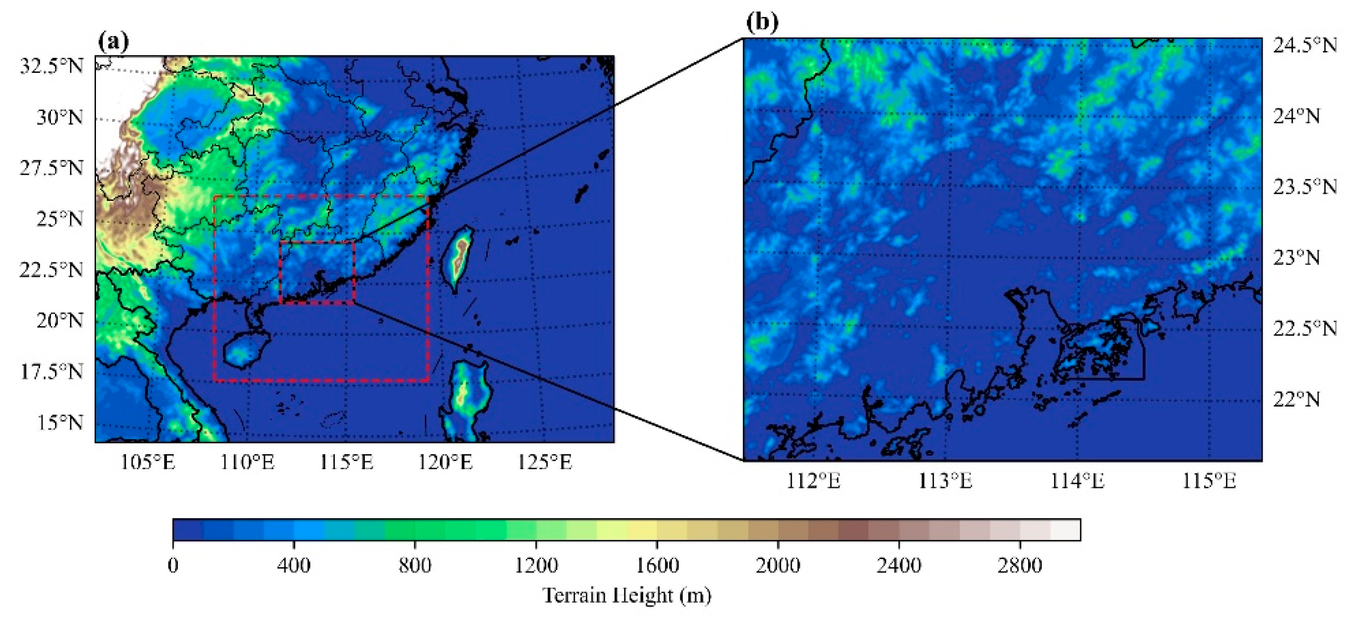
3.1. Overview of the Case

On 6 June 2022, from 16:00 UTC to 22:00 UTC, the PRD experienced a localized convective heavy-rainstorm weather event. The precipitation peak occurred mainly between 18:00 UTC and 22:00 UTC, with the convective system moving eastward and dissipating after 23:00 UTC. This rainstorm event was characterized by strong convective activity, intense short-duration rainfall, localized effects, and rapid development. As depicted in Figure 2, the severe convective process was primarily influenced by the East Asian trough, low-level wind shear, a low-altitude vortex, and a surface mesoscale convergence line (coastal convergence line), which were the result of the combined action of multiple scales and systems. At 18:00 UTC on 6 June 2022, at 500 hPa (Figure 2a), a cold trough extended from the Sea of Japan to the Taiwan Strait, with a cold vortex forming over South China at the trough’s base. At 700 hPa (Figure 2b), a northerly wind transported cold air to South China, following the trough. This cold airflow from the north encountered the warm airflow from the southwest at northern Guangdong and central Fujian, resulting in a confrontation and the formation of a low-level shear line. At 850 hPa (Figure 2c), a low-level vortex formed over South China, exerting a strong convergence effect. In the South China Sea, the significant angle between wind direction and isotherms highlighted the prominence of warm and moist advection, which amassed substantial amounts of water vapor and unstable energy in the lower levels. At 925 hPa (Figure 2d), the low-level vortex and warm moist airflow persisted, with substantial wind speed shear along the coastline, facilitating the triggering of convection.

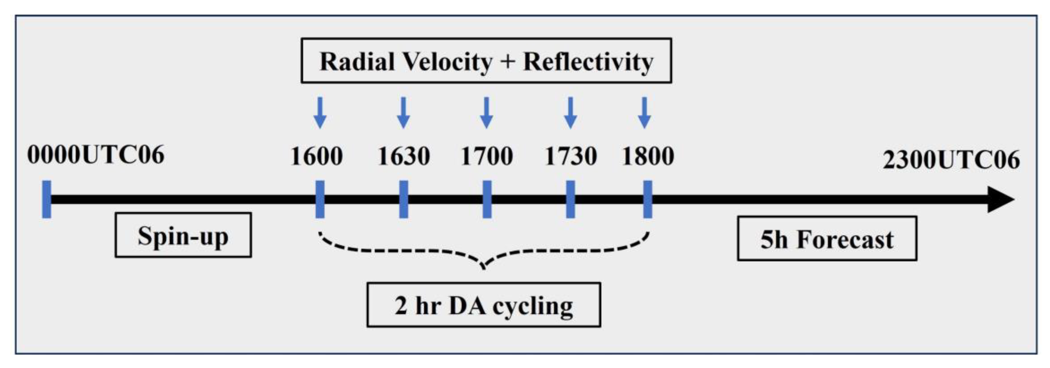
3.2. Model and Experimental Design

In this study, the 4.3 version of the Advanced Research WRF model (ARW-WRF) [36] was used as the NWP model, employing a three-tiered bidirectional nested-grid system with horizontal resolutions of 9 km (319 × 238), 3 km (394 × 340), and 1 km (409 × 334) (Figure 3). The number of vertical layers is 50, with 50 hPa as the model top. To provide initial and boundary conditions for all experiments, the FNL (Final Reanalysis Data) ds083.3 dataset with spatial resolution of 0.25° × 0.25° and a 6 h interval was used. The physical parameterization schemes were set as follows: the WRF Single-Moment 6-class (WSM6) microphysics parameterization scheme [37], the Rapid Radiative Transfer Model (RRTM) longwave radiation scheme [38], the Dudhia shortwave radiation scheme [39], the Yonsei University (YSU) boundary layer scheme [40], the Revised MM5 surface layer scheme [41] and the Unified Noah Land Surface Model [42]. The cumulus parameterization scheme (CPS) employed a Multi-scale Kain–Fritsch scheme (Zheng et al. 2016) [43], which was applied only to the D01 region (Figure 3a).

To evaluate the influence of assimilating SMSR and XPAR RF and RV on the initial conditions and precipitation forecasts, this study arranged four experimental sets (

Table 1. Experiment scheme.

Name	Scheme
CTRL	No DA
DA_S	Assimilating RV and RF of Guangzhou SMSR
DA_X	Assimilating RV and RF of nine XPARs
DA_S_X	Assimilating SMSR and XPARs data sequentially

). The first experiment was a control experiment (CTRL) without radar data assimilation. To mitigate the potential for high correlation between the observation datasets, the second experiment (DA_S) assimilated 3 km resolution SMSR data in both D02 and D03 regions. The third experiment (DA_X) assimilated 3 km resolution XPAR data in D02 and 1 km resolution XPAR data in D03. Furthermore, to delve deeper into the influence of XPAR DA, a DA_S_X experiment was conducted, which sequentially assimilated SMSR and XPAR data.

The control experiment (CTRL) initiated its forecasting at 00:00 UTC on June 6 and continued until 23:00 UTC without the assimilation of radar data. The procedures for the three assimilation experiments are depicted in Figure 4. Forecasting commenced at 00:00 UTC on June 6, with radar data assimilation performing at 30 min intervals during the 2 h period from 16:00 to 18:00 UTC. The experiments concluded with a 5 h deterministic forecast, ending at 23:00 UTC.

4. Data Analysis and Experimental Results

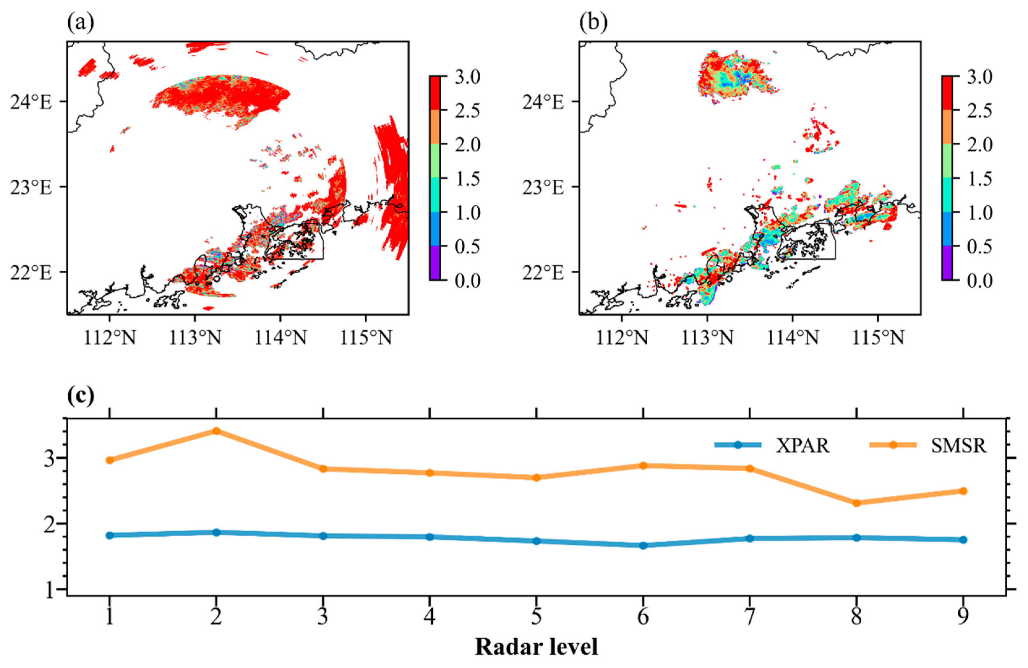
4.1. Radar Data Comparison Analysis

Velocity spectrum width (SW) is a measure of velocity dispersion within a range bin, serving as a tool for quality control of velocity estimates. As SW increases, the reliability of the velocity estimates diminishes. Common meteorological features and conditions, such as near air-mass boundaries and shear regions, can lead to relatively high SW values. From the SW at 1.5° elevation angle at 18:00 UTC on 6 June 2022, for Guangzhou SMSR (Figure 5a) and the nine XPARs (Figure 5b), it is observed that for the XPARs, most SW values are within 2 m/s, with some exceeding 2.5 m/s near convective boundaries, whereas the SW for SMSR is mostly greater than 2.5 m/s, with lower SW values only present within convective regions. Furthermore, the wind field’s response to altitude changes is highly sensitive, leading to a significant increase in SW for SMSR as distance increases, such that the SW at the detection edge of SMSR consistently exceeds 2.5 m/s. The spatial average SW across the first nine elevation angles for both radar (Figure 5c) also indicates that the SW for each elevation angle of SMSR is larger than that of XPAR, by approximately 1.0 m/s. This suggests that, in comparison to SMSR, XPAR exhibits greater spatial accuracy.

4.2. The Analysis Increment in the First Assimilation Cycle

Due to the significant differences in the vertical distribution of the two radar datasets, we conducted an analysis of the average analysis increments across all model layers for the three assimilation experiments (Figure 6) to examine the effects of radar data assimilation vertically. The assimilation of radar data primarily affects the horizontal wind field (UV) (Figure 6a,b) in the atmospheric layers between 6–10 (~925 hPa), 16–18 (~850 hPa), and 24 (~700 hPa), with the absolute average increment of UV for DA_X being consistently smaller than those observed in DA_S and DA_S_X. For temperature (T) (Figure 6c), the assimilation of SMSR data results in a significant warming adjustment, existing mainly lower than the 16th level, while the warming adjustment from XPAR data assimilation is mainly observed below the 10th level, with both adjustments being relatively small in magnitude. The assimilation of radar data affects water vapor (q) (Figure 6d) primarily in the lower 20 levels (middle-to-lower atmosphere), and the increments in DA_X are relatively smaller. This observation underscores the more pronounced impact of assimilating SMSR data on the background field, reflecting its dominant position in the assimilation process. When considering the outcomes of the three assimilation experiments, it becomes evident that the assimilation of XPAR data following SMSR data leads to an enhancement of the assimilation effects, effectively combining the strengths of both.

4.3. Analysis Results

4.3.1. Wind Analysis

Building on the analysis of the vertical distribution of the average increments in the U, V components for each model layer presented in Section 4.2, this section further examines the wind fields at the middle-to-low levels at 18:00 UTC. At 850 hPa (Figure 7), the CTRL experiment predominantly featured southwesterly winds, with stronger winds over land and weaker winds near the land–sea interface, indicating no significant convergence (Figure 7a). DA_S (Figure 7b,e) weakened the extensive southwesterly winds over land, resulting in wind speed shear near the land–sea interface, while DA_X (Figure 7d,f) weakened the wind field near PRE, appropriately retaining the southwesterly winds over central Guangdong. DA_S_X showed stronger sea breezes, with the southwesterly winds over central Guangdong being enhanced compared to DA_S (Figure 7d,g). At 925 and 700 hPa (not displayed), similar adjustment effects were observed across all experiments, with the DA_X experiment exhibiting a more cyclonic wind field after adjustment. This adjustment enhanced the southwesterly winds over central Guangdong, leading to a strong low-level divergence area, which prevented the formation of new convective systems and thus suppressed the further northward development of the convection. The over-adjustment of the wind field in DA_S mainly originates from a large range of wind field errors. The detection range of SMSR is large and its radial velocity detected in 6min is considered as the wind field state at the instantaneous moment. Compared to XPAR, which has a detection period of 2 min, the error of SMSR is much larger, thus resulting in the accumulation of large-scale errors. In general, this error increases with the distance between the observation and the radar.

4.3.2. Radar Echo Analysis

To further analyze the impact of radar data assimilation on the development of convective systems, Figure 8 presents the radar composite reflectivity (CR) at 18:00 UTC in D03. From the SMSR observation, it is evident that at 18:00 UTC, the strong echoes were predominantly distributed along the coastline in a southwest-to-northeast banded pattern. All four experiments effectively simulated the strong convective area along the coastline. The assimilation experiments were able to replicate the strong echo center on the southwestern side of PRE, whereas the echoes on the eastern side were overestimated. This is consistent with the wind field adjustments. The DA_S and DA_S_X experiments, lacking the inhibiting effect of southwest wind divergence, simulated a greater number of false strong echoes (Figure 8c,e).

Figure 9 provides a vertical cross-section of the radar RF along line A (112.7°E, 21.6°N)–B (114.6°E, 23.2°N) at 18:00 UTC. In the SMSR observation, three distinct strong convective centers are evident. The leftmost convective echo top (ET) reaches 8 km near 113°E, with new convection appearing near 113.25°E, and with ET already developing to 6 km; the convection near 113.75°E is stronger, with ET extending to 10 km, and the low-level echo center intensity reaching 55 dBZ. In CTRL (Figure 9b), the left convective ET reaches 8 km, and the convection near PRE is positioned further east and exhibits weaker echo intensity. All assimilation experiments successfully simulate multiple strong convective-echo centers, albeit with slightly lower intensity compared to observation. Following the assimilation of XPAR data, the right convective echo extends to heights of 6–7 km, and the left convection extends to 14 km (Figure 9d). In contrast, after assimilating SMSR data, the left convection reaches a height of 16 km (Figure 9c). However, the DA_X experiment simulates a slightly lower echo-center intensity of 45 dBZ.

4.3.3. Hydrometeor Analysis

This study employs an indirect assimilation method to assimilate radar RF, adjusting the content of hydrometeors in the atmosphere, thereby enhancing the accuracy of precipitation forecast. Therefore, further analysis of the vertical cross-section of $q_r$, $q_g$ and $q_s$ along line AB in the D03 analysis field at 18:00 UTC (Figure 10) is conducted. The positions of the extreme values of hydrometeor mixing ratios correspond to the extreme values of the RF. The vertical distribution of $q_r$ spans from 500 hPa to the surface, with the latitudinal distribution of $q_r$ in CTRL ranging from 113.12°E to 113.33°E. In assimilation experiments, $q_r$ is distributed around 113.12°E–113.33°E, 113.5°E, and 114.17°E (Figure 10a). In DA_S (Figure 10b), the maximum $q_r$ is distributed around 113.12°E–113.33°E, reaching 4.7 g/kg; in DA_X (Figure 10c), the maximum is around 113.5°E, reaching 2.8 g/kg; and in DA_S_X (Figure 10d), the maximum is around 114.17°E, reaching 3.8 g/kg. In CTRL, the latitudinal distribution range of $q_s$ and $q_g$ is similar, primarily around 113.12°E–113.33°E, extending vertically from 600 hPa to 300 hPa, with maximum values of 1.4 and 2.4 g/kg, respectively (Figure 10e,i). After assimilating SMSR or XPAR data, $q_s$ and $q_g$ can extend to 100 hPa, with maximum values reaching 3.0 and 4.1 g/kg, respectively (Figure 10f,j). In DA_S_X, the maximum values of $q_s$ and $q_g$ reach 3.6 and 4.0 g/kg, respectively, which are 2.2 and 1.6 g/kg higher than those in CTRL (Figure 10h,l). Compared to DA_X, the analysis fields of DA_S and DA_S_X have larger extreme values and wider ranges for each type of hydrometeor.

4.4. Forecasting Results

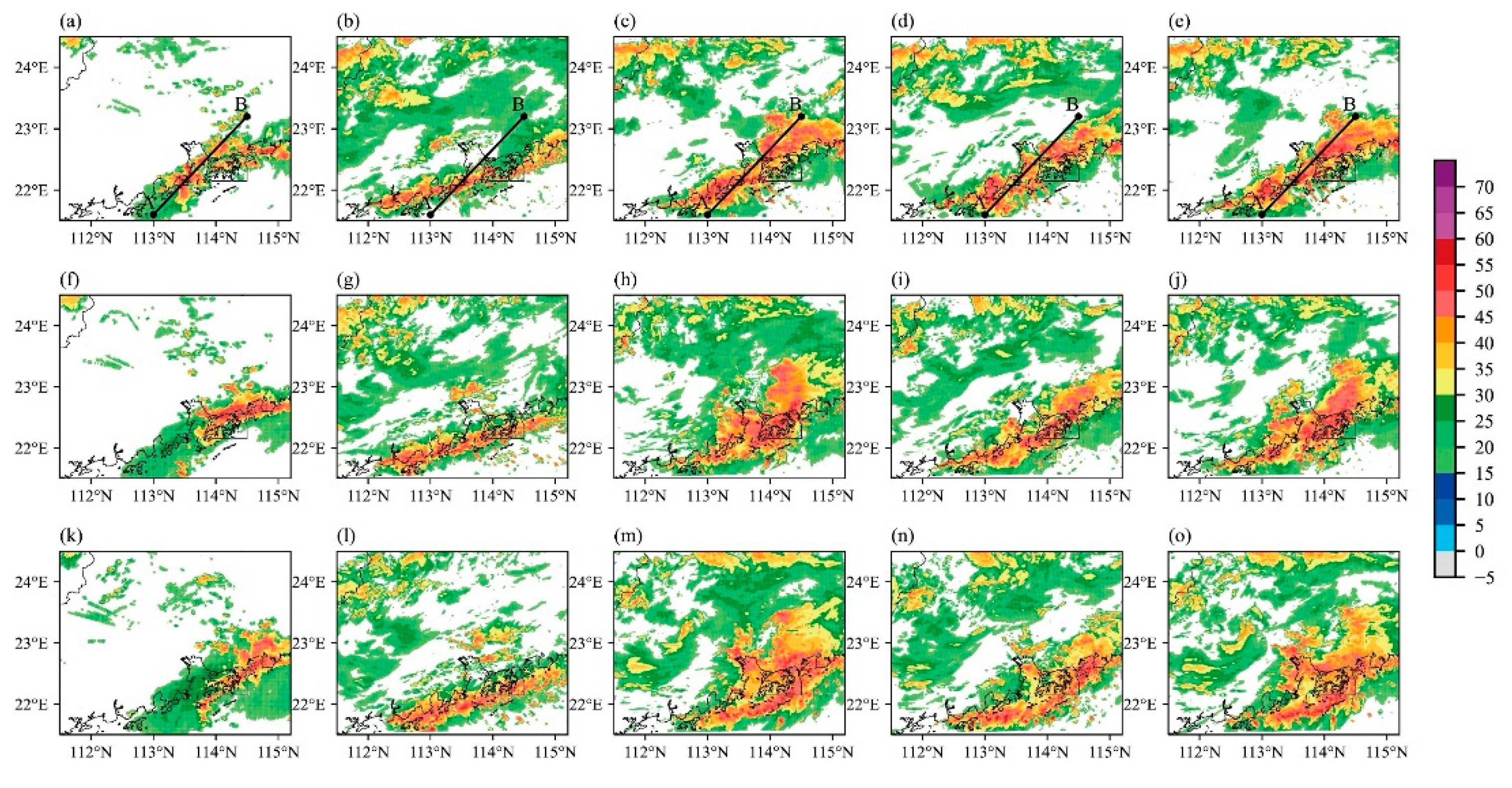
4.4.1. Composite Reflectivity Forecast

To assess the influence of radar DA on the prediction of convective evolution and its movement, Figure 11 illustrates the CR from 19:00 UTC to 21:00 UTC on 6 June 2022. The radar echo core of the strong convective event is situated in the PRD region and is moving eastward (Figure 11a,f,k). In CTRL, the CR exhibits an east–west banded structure, which deviates from observation and does not align with the eastward movement observed in the SMSR data over time (Figure 11b,g,l). DA_S forecasts widespread false echoes in the vicinity of PRE and its northeastern inland areas (Figure 11c,h,m). In comparison, DA_X exhibits a more-aligned pattern with the SMSR observation in the northeastern side of PRE, but there are still false echoes present in the southwestern sea area at 20:00 UTC and 21:00 UTC (Figure 11d,i,n). Additionally, compared to DA_S, DA_S_X shows a reduction in the intensity and extent of the false echoes in the northeastern side of PRE (Figure 11e,j,o).

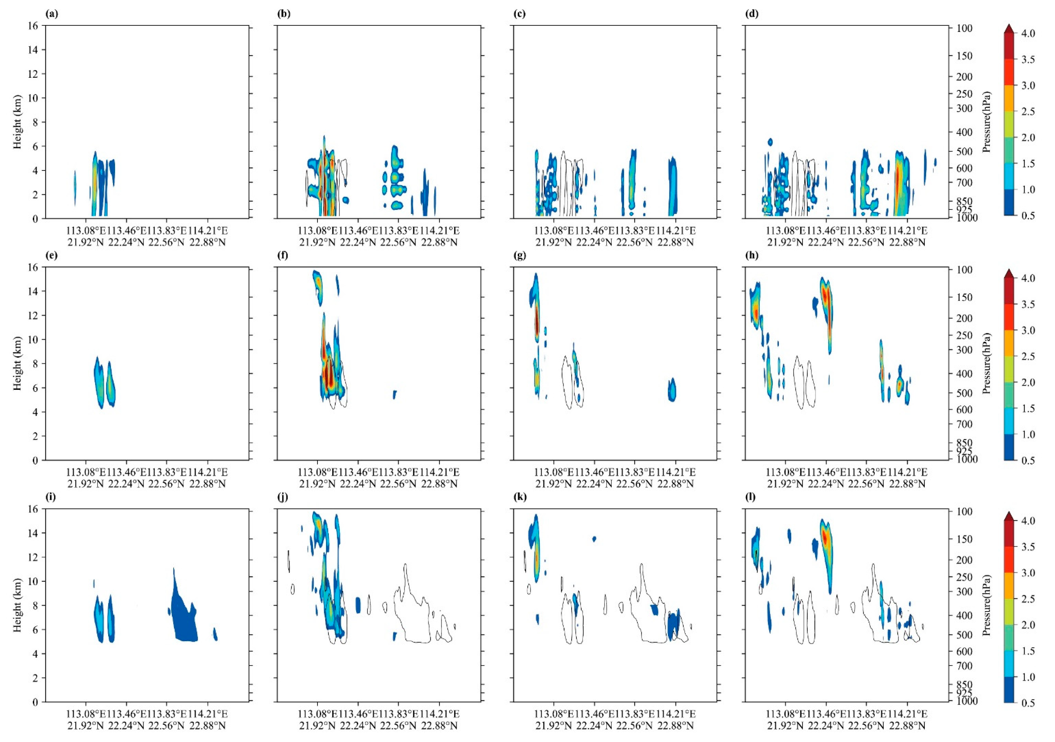
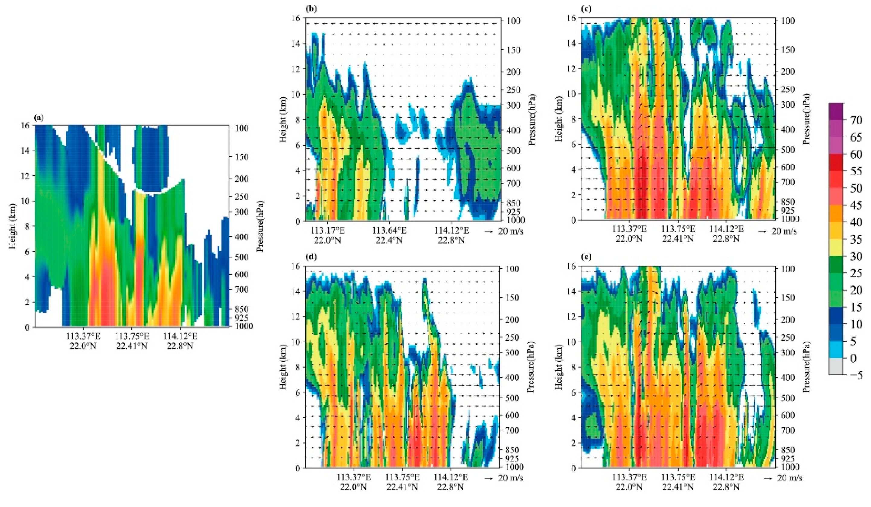
4.4.2. Vertical Structure Analysis

Further analysis of the radar echo intensity and vertical wind-field structure of the convective system at 19:00 is provided in Figure 12. In CTRL (Figure 12b), the wind field was primarily horizontal, with strong radar echoes appearing near 113.5°E, although the echo intensity was weaker compared to the SMSR observation (Figure 12a), reaching 45 dBZ. And no strong echoes were generated near 114.0°E. Following the assimilation of SMSR data (Figure 12c), strong-echo centers emerged within the range of 113.4°E to 114.1°E, with the central echo intensity being slightly stronger than the SMSR observation, reaching 55 dBZ. The echo top height was higher than the observation, reaching 16 km, accompanied by intense updrafts, with wind speed reaching 12 m/s. The radar echoes resulting from the assimilation of XPAR data were similar to the observation within the range of 113.4°E to 114.1°E, with the strong-echo top height near 113.8°E ranging between 10 and 12 km (Figure 12d). Compared to DA_S, DA_S_X showed weakened echo intensity near 114.3°E, but the strong-echo center within the range of 113.4°E to 114.1°E remained relatively stronger than the observation, with significant updrafts (Figure 12e).

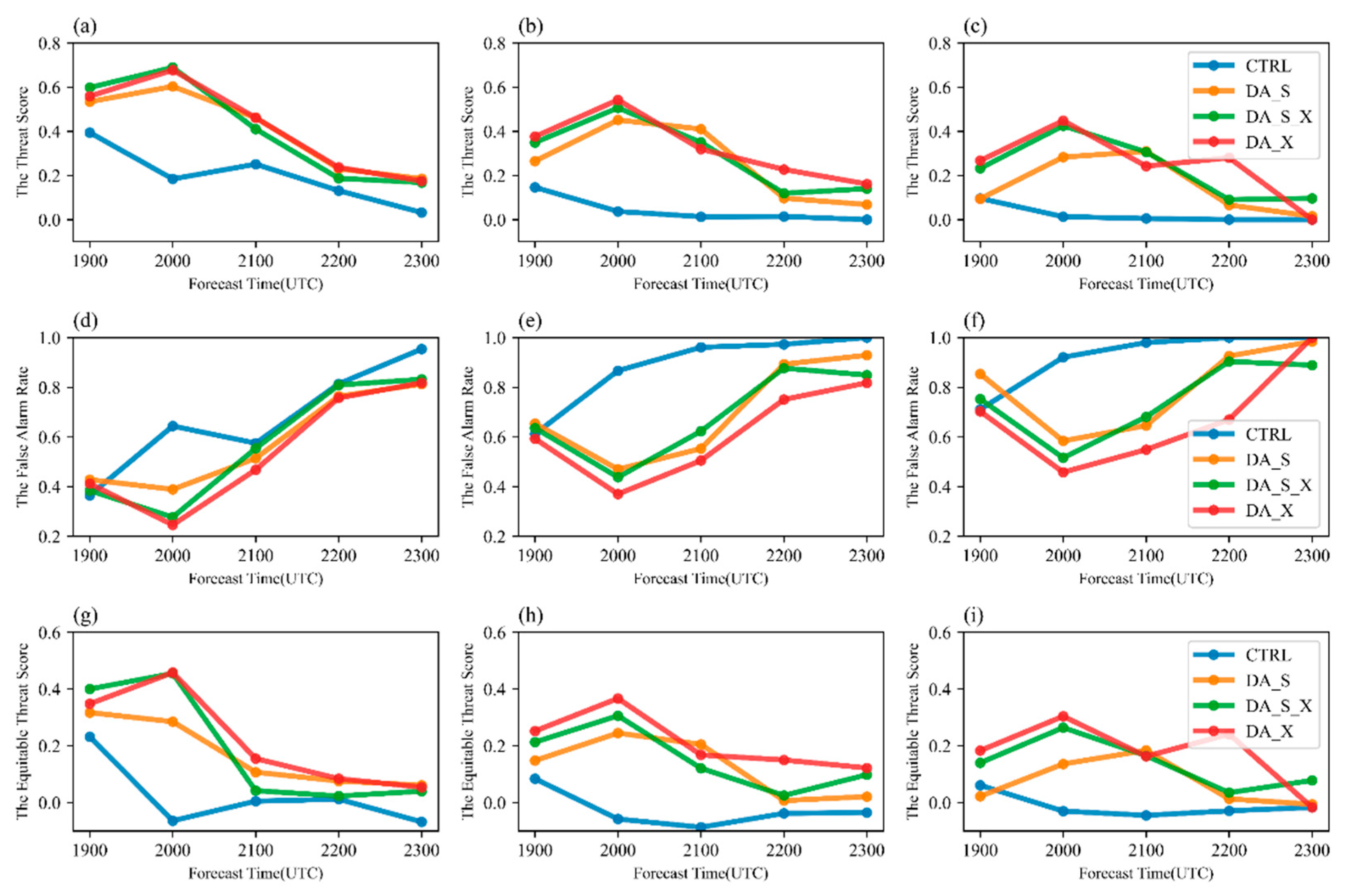
4.4.3. Precipitation Forecast

The rainband of this event was primarily located along the coastal areas of PRD and moved rapidly from west to east. In CTRL (Figure 13e–h), the rainband was mainly situated at the land–sea interface, showing an east–west trend and no significant movement, primarily caused by wind shear. Assimilation of the radar data resulted in a significant adjustment of the forecast for the area of heavy precipitation, with an increase in the localization of precipitation, covering the area of observed precipitation and moving significantly to the east. Among these, DA_S overestimated the precipitation over the eastern side of PRE and had false alarms, mainly due to the excessive weakening of the southwest flow by assimilating SMSR data, which favored low-level wind convergence on the northeastern side of the convective region, promoting continued convective development towards the northeast (Figure 13i–l). DA_X had a more consistent forecast of hourly precipitation patterns and intensities with the actual observations (Figure 13m–p). Notably, the range of false alarms in DA_S_X was reduced (Figure 13q–t). This indicates that, after assimilating XPAR data, it can suppress the excessive adjustment of the local heavy-precipitation environment field by the SMSR data assimilation, thereby improving the forecasting of local heavy precipitation.

To quantitatively evaluate the accuracy of hourly precipitation forecasts, we calculated the Threat Score (TS) and Equitable Threat Score (ETS) for each experiment in the D03 region for hourly precipitation from 18:00 to 22:00 (Figure 14).

$$TS={\displaystyle \frac{NA}{NA+NB+NC }},$$

(6)

$$FAR={\displaystyle \frac{NC}{NA+NC}},$$

(7)

$$Dr={\displaystyle \frac{\left(NA+NB\right)\times \left(NA+NC\right)}{NA+NB+NC+ND}},$$

(8)

$$ETS={\displaystyle \frac{NA-Dr}{NA+NB+NC-Dr}},$$

(9)

$NA$ represents the precipitation predicted by the WRF model and observed by the reference data; $NB$ represents the precipitation not predicted by the WRF model but observed by the reference data; $NC$ represents the precipitation predicted by the WRF model but not observed by the reference data; and $ND$ represents the precipitation not predicted by the WRF model and not observed by the reference data. For TS and ETS, 1 was the best score, and 0 was the worst. For FAR, 0 was the best.

The TS/ETS of each assimilation experiment is higher than that of the control, indicating that the assimilation of radar data effectively improves the accuracy of precipitation forecasts in this case. Comparing DA_S and DA_S_X, the assimilation of XPAR data enhances the forecasting effectiveness of the DA_S experiment for heavy-precipitation events with hourly precipitation rates exceeding 10 mm (Figure 14c,i). Among them, DA_X achieved the highest TS and ETS for forecasts of precipitation across different intensity levels, showing the most significant improvement over the control experiment. Furthermore, the FAR of precipitation in the assimilation tests is found to be significantly smaller than in the control, indicating that assimilating radar data effectively improved the precipitation fallout area (Figure 13). Additionally, the FAR of DA_S is found to be higher than that of DA_X, which further indicates that the over-adjustment of the wind field by assimilating SMSR data caused more false precipitation (Figure 14d–f). It is noteworthy that the TS/ETS of all assimilation experiments exhibited an increase from 19:00 to 20:00. This phenomenon may be attributed to the reasonable adjustment of the low-level wind field by the assimilated radar data, which resulted in a more accurate representation of convection over the subsequent two hours. Consequently, the convective-precipitation forecasts demonstrated enhanced precision. The forecast error increases over time, resulting in a gradual decrease in TS/ETS over the subsequent three hours.

5. Summary

This study selected a rainstorm weather event that occurred on 6 June 2022, in the Pearl River Delta region. Based on the Weather Research and Forecasting (WRF) model and its Data Assimilation System (WRFDA), two different radar datasets were assimilated using a three-dimensional variational (3Dvar) approach within a convection-allowing grid. The main results and conclusions are as follows:

While SMSR data dominate with respect to coverage, XPAR data exhibit greater accuracy. For the analyzed local-rainstorm event, the assimilation of SMSR data led to excessive adjustments in the middle to low-level wind fields, causing an overdevelopment of convection and an unnecessarily high content of hydrometeors in the clouds, which resulted in the generation of extensive false echoes. The assimilation of XPAR data, on the other hand, produced more reasonable adjustments to the middle-to-low-level wind fields, creating small-to-medium-scale horizontal convergence in the analysis field. Sequentially assimilating SMSR and XPAR data mitigated the excessive wind-field adjustments caused by the assimilation of SMSR data alone. This highlights the advantage of the high spatial accuracy of XPAR data. In terms of forecast outcomes, the assimilation of XPAR data led to predictions of composite reflectivity, radar echoes, and hourly precipitation that were more in line with observations. Sequentially assimilating SMSR and XPAR data reduced the false precipitation forecasts seen in the SMSR assimilation experiment alone, significantly enhancing the forecast skill for heavy rain (>10 mm/h). This demonstrates the critical importance of assimilating XPAR data in improving the simulation capabilities of local severe convective weather systems and the accuracy of quantitative precipitation forecasts for rainstorms.

The question of whether radar data with a resolution of 30 m is more valuable than that with a resolution of 250 m for models with grid resolutions of 1 or 3 km has been a subject of contention. The findings of this study unequivocally demonstrate that ultra-high-resolution XPAR data are indeed valuable, primarily due to two key reasons. Firstly, XPAR provides significantly denser data in a vertical orientation, approximately seven times that of SMSR, which adapts to the demands of the model’s vertical layer structure. This enhanced vertical density facilitates more precise adjustments of variables within the model space. Secondly, XPAR offers more accurate observation, significantly reducing observational errors. This accuracy is a result of not only the high temporal resolution (bringing the data closer to the assimilation time), but also the superior spatial resolution. To further substantiate this conclusion, future research will involve the analysis of additional case studies.

References

1. Zhang, A.; Xiao, L.; Min, C.; Chen, S.; Kulie, M.; Huang, C.; Liang, Z. Evaluation of Latest GPM-Era High-Resolution Satellite Precipitation Products during the May 2017 Guangdong Extreme Rainfall Event. Atmos. Res. 2019, 216, 76–85. [Google Scholar] [CrossRef]
2. Aksoy, A.; Dowell, D.C.; Snyder, C. A Multicase Comparative Assessment of the Ensemble Kalman Filter for Assimilation of Radar Observations. Part I: Storm-Scale Analyses. Mon. Weather. Rev. 2009, 137, 1805–1824. [Google Scholar] [CrossRef]
3. Shen, F.; Xu, D.; Min, J.; Chu, Z.; Li, X. Assimilation of Radar Radial Velocity Data with the WRF Hybrid 4DEnVar System for the Prediction of Hurricane Ike (2008). Atmos. Res. 2020, 234, 104771. [Google Scholar] [CrossRef]
4. Fabry, F.; Meunier, V. Why Are Radar Data so Difficult to Assimilate Skillfully? Mon. Weather. Rev. 2020, 148, 2819–2836. [Google Scholar] [CrossRef]
5. Shen, F.; Song, L.; He, Z.; Xu, D.; Chen, J.; Huang, L. Impacts of Adding Hydrometeor Control Variables on the Radar Reflectivity Data Assimilation for the 6–8 August 2018 Mesoscale Convective System Case. Atmos. Res. 2023, 295, 107012. [Google Scholar] [CrossRef]
6. Zheng, H.; Chen, Y.; Zheng, S.; Meng, D.; Sun, T. Radar Reflectivity Assimilation Based on Hydrometeor Control Variables and Its Impact on Short-Term Precipitation Forecasting. Remote Sens. 2023, 15, 672. [Google Scholar] [CrossRef]
7. Wang, C.; Chen, M.; Chen, Y. Impact of Combined Assimilation of Wind Profiler and Doppler Radar Data on a Convective-Scale Cycling Forecasting System. Mon. Weather Rev. 2022, 150, 431–450. [Google Scholar] [CrossRef]
8. Xu, D.; Yang, G.; Wu, Z.; Shen, F.; Li, H.; Zhai, D. Evaluate Radar Data Assimilation in Two Momentum Control Variables and the Effect on the Forecast of Southwest China Vortex Precipitation. Remote Sens. 2022, 14, 3460. [Google Scholar] [CrossRef]
9. Shen, F.; Xu, D.; Min, J. Effect of Momentum Control Variables on Assimilating Radar Observations for the Analysis and Forecast for Typhoon Chanthu (2010). Atmos. Res. 2019, 230, 104622. [Google Scholar] [CrossRef]
10. Shen, F.; Shu, A.; Liu, Z.; Li, H.; Jiang, L.; Zhang, T.; Xu, D. Assimilating FY-4A AGRI Radiances with a Channel-Sensitive Cloud Detection Scheme for the Analysis and Forecasting of Multiple Typhoons. Adv. Atmos. Sci. 2024, 41, 937–958. [Google Scholar] [CrossRef]
11. Xu, D.; Shen, F.; Min, J. Effect of Background Error Tuning on Assimilating Radar Radial Velocity Observations for the Forecast of Hurricane Tracks and Intensities. Meteorol. Appl. 2020, 27, e1820. [Google Scholar] [CrossRef]
12. Zhang, G.; Mahale, V.N.; Putnam, B.J.; Qi, Y.; Cao, Q.; Byrd, A.D.; Bukovcic, P.; Zrnic, D.S.; Gao, J.; Xue, M.; et al. Current Status and Future Challenges of Weather Radar Polarimetry: Bridging the Gap between Radar Meteorology/Hydrology/Engineering and Numerical Weather Prediction. Adv. Atmos. Sci. 2019, 36, 571–588. [Google Scholar] [CrossRef]
13. Zrnic, D.S.; Kimpel, J.F.; Forsyth, D.E.; Shapiro, A.; Crain, G.; Ferek, R.; Heimmer, J.; Benner, W.; McNellis, F.T.J.; Vogt, R.J. Agile-Beam Phased Array Radar for Weather Observations. Bull. Am. Meteorol. Soc. 2007, 88, 1753–1766. [Google Scholar] [CrossRef]
14. Stratman, D.R.; Yussouf, N.; Jung, Y.; Supinie, T.A.; Xue, M.; Skinner, P.S.; Putnam, B.J. Optimal Temporal Frequency of NSSL Phased Array Radar Observations for an Experimental Warn-on-Forecast System. Weather. Forecast. 2020, 35, 193–214. [Google Scholar] [CrossRef]
15. Chandrasekar, V.; Mclaughlin, D.; Zink, M. The CASA IP1 Test-Bed after 5 Years Operation: Accomplishments, Breakthroughs, Challenges and Lessons. In Proceedings of the 6th European Conference on Radar in Meteorology and Hydrology: Advances in Radar Technology, Sibiu, Romania, 6–10 September 2010; ERAD: Sibiu, Romania, 2010. [Google Scholar]
16. Zhang, X.; Huang, X.; Liu, X.A.; Lu, J.; Geng, L.; Huang, H.; Zhen, G. The Hazardous Convective Storm Monitoring of Phased-Array Antenna Radar at Daxing International Airport of Beijing. J. Appl. Meteorol. Sci. 2022, 33, 192–204. [Google Scholar]
17. Lin, X.; Feng, Y.; Xu, D.; Jian, Y.; Huang, F.; Huang, J. Improving the Nowcasting of Strong Convection by Assimilating Both Wind and Reflectivity Observations of Phased Array Radar: A Case Study. J. Meteorol. Res. 2022, 36, 61–78. [Google Scholar] [CrossRef]
18. Huang, Y.; Wang, X.; Kerr, C.; Mahre, A.; Yu, T.-Y.; Bodine, D. Impact of Assimilating Future Clear-Air Radial Velocity Observations from Phased-Array Radar on a Supercell Thunderstorm Forecast: An Observing System Simulation Experiment Study. Mon. Weather Rev. 2020, 148, 3825–3845. [Google Scholar] [CrossRef]
19. Yussouf, N.; Stensrud, D.J. Impact of Phased-Array Radar Observations over a Short Assimilation Period: Observing System Simulation Experiments Using an Ensemble Kalman Filter. Mon. Wea. Rev. 2010, 138, 517–538. [Google Scholar] [CrossRef]
20. Huang, Y.; Wang, X.; Mahre, A.; Yu, T.-Y.; Bodine, D. Impacts of Assimilating Future Clear-Air Radial Velocity Observations from Phased Array Radar on Convection Initiation Forecasts: An Observing System Simulation Experiment Study. Mon. Weather. Rev. 2022, 150, 1563–1583. [Google Scholar] [CrossRef]
21. Ming, J.; Gong, P.; Lu, Y.; Zhao, K.; Huang, H.; Chen, X.; Wang, S.; Zhang, Q. Impact of Assimilating C-Band Phased-Array Radar Data With EnKF on the Forecast of Convection Initiation: A Case Study in Beijing, China. J. Geophys. Res. Atmos. 2023, 128, e2023JD038542. [Google Scholar] [CrossRef]
22. Wang, C.; Zhao, K.; Zhu, K.; Huang, H.; Lu, Y.; Yang, Z.; Fu, P.; Zhang, Y.; Chen, B.; Hu, D. Assimilation of X-Band Phased-Array Radar Data With EnKF for the Analysis and Warning Forecast of a Tornadic Storm. J. Adv. Model. Earth Syst. 2021, 13, e2020MS002441. [Google Scholar] [CrossRef]
23. Helmus, J.J.; Collis, S.M. The Python ARM Radar Toolkit (Py-ART), a Library for Working with Weather Radar Data in the Python Programming Language. J. Open Res. Softw. 2016, 4, 25. [Google Scholar] [CrossRef]
24. Wang, Y.; Wang, X. Development of Convective-Scale Static Background Error Covariance within GSI-Based Hybrid EnVar System for Direct Radar Reflectivity Data Assimilation. Mon. Weather. Rev. 2021, 149, 2713–2736. [Google Scholar] [CrossRef]
25. Johnson, A.; Wang, X.; Carley, J.R.; Wicker, L.J.; Karstens, C. A Comparison of Multiscale GSI-Based EnKF and 3DVar Data Assimilation Using Radar and Conventional Observations for Midlatitude Convective-Scale Precipitation Forecasts. Mon. Weather. Rev. 2015, 143, 3087–3108. [Google Scholar] [CrossRef]
26. Barker, D.M.; Huang, W.; Guo, Y.-R.; Bourgeois, A.J.; Xiao, Q.N. A Three-Dimensional Variational Data Assimilation System for MM5: Implementation and Initial Results. Mon. Weather. Rev. 2004, 132, 897–914. [Google Scholar] [CrossRef]
27. Barker, D.; Huang, X.-Y.; Liu, Z.; Auligné, T.; Zhang, X.; Rugg, S.; Ajjaji, R.; Bourgeois, A.; Bray, J.; Chen, Y.; et al. The Weather Research and Forecasting Model’s Community Variational/Ensemble Data Assimilation System: WRFDA. Bull. Am. Meteorol. Soc. 2012, 93, 831–843. [Google Scholar] [CrossRef]
28. Parrish, D.F.; Derber, J.C. The National Meteorological Center’s Spectral Statistical-Interpolation Analysis System. Mon. Weather. Rev. 1992, 120, 1747–1763. [Google Scholar] [CrossRef]
29. Tong, M.; Xue, M. Ensemble Kalman Filter Assimilation of Doppler Radar Data with a Compressible Nonhydrostatic Model: OSS Experiments. Mon. Weather. Rev. 2005, 133, 1789–1807. [Google Scholar] [CrossRef]
30. Wang, H.; Sun, J.; Fan, S.; Huang, X.-Y. Indirect Assimilation of Radar Reflectivity with WRF 3D-Var and Its Impact on Prediction of Four Summertime Convective Events. J. Appl. Meteorol. Climatol. 2013, 52, 889–902. [Google Scholar] [CrossRef]
31. Shen, F.; Min, J.; Li, H.; Xu, D.; Shu, A.; Zhai, D.; Guo, Y.; Song, L. Applications of Radar Data Assimilation with Hydrometeor Control Variables within the WRFDA on the Prediction of Landfalling Hurricane IKE (2008). Atmosphere 2021, 12, 853. [Google Scholar] [CrossRef]
32. Gao, J.; Stensrud, D.J. Assimilation of Reflectivity Data in a Convective-Scale, Cycled 3DVAR Framework with Hydrometeor Classification. J. Atmos. Sci. 2012, 69, 1054–1065. [Google Scholar] [CrossRef]
33. Lin, Y.-L.; Farley, R.D.; Orville, H.D. Bulk Parameterization of the Snow Field in a Cloud Model. J. Clim. Appl. Meteorol. 1983, 22, 1065–1092. [Google Scholar] [CrossRef]
34. Gilmore, M.S.; Straka, J.M.; Rasmussen, E.N. Precipitation and Evolution Sensitivity in Simulated Deep Convective Storms: Comparisons between Liquid-Only and Simple Ice and Liquid Phase Microphysics. Mon. Weather. Rev. 2004, 132, 1897–1916. [Google Scholar] [CrossRef]
35. Dowell, D.C.; Wicker, L.J.; Snyder, C. Ensemble Kalman Filter Assimilation of Radar Observations of the 8 May 2003 Oklahoma City Supercell: Influences of Reflectivity Observations on Stormscale Analyses. Mon. Weather. Rev. 2011, 139, 272–294. [Google Scholar] [CrossRef]
36. Skamarock, W.C.; Klemp, J.B. A Time-Split Nonhydrostatic Atmospheric Model for Weather Research and Forecasting Applications. J. Comput. Phys. 2008, 227, 3465–3485. [Google Scholar] [CrossRef]
37. Hong, S.Y.; Lim, J.O.J. The WRF Single-Moment 6-Class Microphysics Scheme (WSM6). Asia Pac. J. Atmos. Sci. 2006, 42, 129–151. [Google Scholar]
38. Mlawer, E.J.; Taubman, S.J.; Brown, P.D.; Iacono, M.J.; Clough, S.A. Radiative Transfer for Inhomogeneous Atmospheres: RRTM, a Validated Correlated-k Model for the Longwave. J. Geophys. Res. 1997, 102, 16663–16682. [Google Scholar] [CrossRef]
39. Dudhia, J. Numerical Study of Convection Observed during the Winter Monsoon Experiment Using a Mesoscale Two-Dimensional Model. J. Atmos. Sci. 1989, 46, 3077–3107. [Google Scholar] [CrossRef]
40. Hong, S.-Y.; Noh, Y.; Dudhia, J. A New Vertical Diffusion Package with an Explicit Treatment of Entrainment Processes. Mon. Weather Rev. 2006, 134, 2318–2341. [Google Scholar] [CrossRef]
41. Jiménez, P.A.; Dudhia, J.; González-Rouco, J.F.; Navarro, J.; Montávez, J.P.; García-Bustamante, E. A Revised Scheme for the WRF Surface Layer Formulation. Mon. Weather Rev. 2012, 140, 898–918. [Google Scholar] [CrossRef]
42. Tewari, M.; Wang, W.; Dudhia, J.; Lemone, M.A.; Mitchell, K.; Ek, M.; Gayno, G.; Wegiel, J.; Cuenca, R. Implementation and Verification of the Unified NOAH Land Surface Mode in the WRF Model. In Proceedings of the 20th Conference on Weather Analysis and Forecasting/16th Conference on Numerical Weather Prediction, Seattle, WA, USA, 11–15 January 2004; pp. 12–16. [Google Scholar]
43. Zheng, Y.; Alapaty, K.; Herwehe, J.A.; Del Genio, A.D.; Niyogi, D. Improving High-Resolution Weather Forecasts Using the Weather Research and Forecasting (WRF) Model with an Updated Kain–Fritsch Scheme. Mon. Weather. Rev. 2016, 144, 833–860. [Google Scholar] [CrossRef]
Figure 1. (a) Location of Guangzhou SMSR (red pentagram) and nine XPARs in Guangdong Province (blue triangles), with the radar-coverage circles in 230 (solid red circle) and 60/40 (blue dashed circles) km ranges for SMSR and XPAR, respectively. The black dashed frame delineates the D03. (b) The position of automatic weather stations across Guangdong Province (green scatters).
Remotesensing 16 02655 g001
Figure 2. The potential geopotential height field (black contours, units: dagpm), temperature field (red contours, units: °C), wind field (wind barbs, units: m/s), and relative humidity field (shaded areas) from the ERA5 reanalysis data at 18:00 UTC on 6 June 2022 are depicted at different pressure levels: (a) 500 hPa; (b) 700 hPa; (c) 850 hPa; (d) 925 hPa. “D” in red represents the center of the cyclone. The brown line represents the wind shear line.
Remotesensing 16 02655 g002
Figure 3. Model grid configuration and topography (shaded). (a) Domain configuration; (b) D03 configuration.
Remotesensing 16 02655 g003
Figure 4. The flow chart for the DA experiments.
Remotesensing 16 02655 g004
Figure 5. Velocity spectrum width (SW) at 1.5° elevation angle for (a) SMSR and (b) XPARs. And (c) the spatial average velocity SW from the lowest to the highest of the first 9 elevation angles for both at 18:00 UTC on 6 June 2022. Unit: m/s.
Remotesensing 16 02655 g005
Figure 6. The average analysis increment in each model layer for the first assimilation cycle in the D03 region: (a) u (units: m/s), (b) v (units: m/s), (c) T (units: 10−3 K), (d) q (units: g/kg).
Remotesensing 16 02655 g006
Figure 7. The first row shows the 850hPa horizontal wind field (vector) and wind speed (shaded, units: m/s) at 18:00 UTC on 6 June 2022, for (a) CTRL, (b) DA_S, (c) DA_X, and (d) DA_S_X. The second row depicts the incremental field of the horizontal wind field relative to CTRL, with wind speed greater than 5 m/s indicated by a red vector, for (e) DA_S, (f) DA_X, and (g) DA_S_X.
Remotesensing 16 02655 g007
Figure 8. Radar composite reflectivity-analysis field at 18:00 UTC in D03 on 6 June 2022, for (a) OBS-SMSR, (b) CTRL, (c) DA_S, (d) DA_X, and (e) DA_S_X; line AB is the profile in Figure 9 and Figure 10.
Remotesensing 16 02655 g008
Figure 9. Vertical cross-sections of RF (shaded, units: dBZ) along the black solid line A (112.7°E, 21.6°N) and B (114.6°E, 23.2°N) in Figure 8 at 18:00 UTC on 6 June 2022. (a) OBS-SMSR, (b) CTRL, (c) DA_S, (d) DA_X, (e) DA_S_X. The height is from sea level.
Remotesensing 16 02655 g009
Figure 10. Vertical cross-sections of q r   (first row), q g (second row), and q s (third row) along line AB for each experiment at 18:00 UTC on 6 June 2022. (a,e,i) CTRL, (b,f,j) DA_S, (c,g,k) DA_X, (d,h,l) DA_S_X. The black contours represent the distribution of hydrometeors in CTRL. The height is from sea level.
Remotesensing 16 02655 g010
Figure 11. Composite reflectivity at 19:00 UTC (first row), 20:00 UTC (second row), and 21:00 UTC (third row) on 6 June 2022 (units: dBZ). (a,f,k) OBS-SMSR, (b,g,l) CTRL, (c,h,m) DA_S, (d,i,n) DA_X, (e,j,o) DA_S_X.
Remotesensing 16 02655 g011
Figure 12. Vertical cross-sections of RF (shaded, units: dBZ) and wind (vector) along the black solid line A (113.0°E, 21.6°N) and B (114.5°E, 23.2°N) in Figure 11 at 19:00 UTC on 6 June 2022. (a) OBS-SMSR, (b) CTRL, (c) DA_S, (d) DA_X, (e) DA_S_X. The height is from sea level.
Remotesensing 16 02655 g012
Figure 13. Hourly precipitation from 18:00 UTC (first column) to 22:00 (last column) on 6 June 2022 (units: mm). (ad) OBS, (eh) CTRL, (il) DA_S, (mp) DA_X, (qt) DA_S_X.
Remotesensing 16 02655 g013
Figure 14. Threat Score (TS) (first row), False Alarm Rate (FAR) (second row) and Equitable Threat Score (ETS) (third row) for hourly precipitation from 18:00 to 22:00 on 6 June 2022 (a,d,g) for >1 mm, (b,e,h) for >5 mm, (c,f,i) for >10 mm.
Remotesensing 16 02655 g014