Article

CACM-Net: Daytime Cloud Mask for AGRI Onboard the FY-4A Satellite

1
School of Marine Sciences and Technology, Zhejiang Ocean University, Zhoushan 316022, China
2
School of Electronic and Information Engineering, Nanjing University of Information Science and Technology, Nanjing 210044, China
3
SANYA Oceanographic Laboratory, Sanya 572000, China
4
School of Marine Sciences, Nanjing University of Information Science and Technology, Nanjing 210044, China
5
School of Software, Nanjing University of Information Science and Technology, Nanjing 210044, China
6
Fujian Meteorological Disaster Prevention Technology Center, Fuzhou 350007, China
7
Fujian Institute of Meteorological Sciences, Fuzhou 350007, China
*
Author to whom correspondence should be addressed.
Remote Sens. 2024, 16(14), 2660; https://doi.org/10.3390/rs16142660 (registering DOI)
Submission received: 5 June 2024 / Revised: 12 July 2024 / Accepted: 12 July 2024 / Published: 20 July 2024

Abstract

:
Accurate cloud detection is a crucial initial stage in optical satellite remote sensing. In this study, a daytime cloud mask model is proposed for the Advanced Geostationary Radiation Imager (AGRI) onboard the Fengyun 4A (FY-4A) satellite based on a deep learning approach. The model, named “Convolutional and Attention-based Cloud Mask Net (CACM-Net)”, was trained using the 2021 dataset with CALIPSO data as the truth value. Two CACM-Net models were trained based on a satellite zenith angle (SZA) < 70° and >70°, respectively. The study evaluated the National Satellite Meteorological Center (NSMC) cloud mask product and compared it with the method established in this paper. The results indicate that CACM-Net outperforms the NSMC cloud mask product overall. Specifically, in the SZA < 70° subset, CACM-Net enhances accuracy, precision, and F1 score by 4.8%, 7.3%, and 3.6%, respectively, while reducing the false alarm rate (FAR) by approximately 7.3%. In the SZA > 70° section, improvements of 12.2%, 19.5%, and 8% in accuracy, precision, and F1 score, respectively, were observed, with a 19.5% reduction in FAR compared to NSMC. An independent validation dataset for January–June 2023 further validates the performance of CACM-Net. The results show improvements of 3.5%, 2.2%, and 2.8% in accuracy, precision, and F1 scores for SZA < 70° and 7.8%, 11.3%, and 4.8% for SZA > 70°, respectively, along with reductions in FAR. Cross-comparison with other satellite cloud mask products reveals high levels of agreement, with 88.6% and 86.3% matching results with the MODIS and Himawari-9 products, respectively. These results confirm the reliability of the CACM-Net cloud mask model, which can produce stable and high-quality FY-4A AGRI cloud mask results.

1. Introduction

Cloud cover attenuates or even loses feature information captured by remote sensing imagery [1]. However, meteorologists rely on cloud features in remote sensing images to analyze the birth and disappearance patterns of meteorological phenomena. A cloud mask is a crucial product in remote sensing image processing, as it serves as the foundation for global cloud coverage [2]. It is also a primary component for subsequent tasks, such as cloud rejection, cloud classification, fog detection, and extreme weather forecasting and warning. Accurate detection of cloud distribution characteristics in remote sensing images is crucial for efficient and precise observation using remote sensing technology.
Polar-orbiting satellites are used to analyze land surface information at extremely high spatial resolutions but cannot continuously monitor the same area. In contrast, geostationary satellites positioned along the equator at fixed longitudes can sample at higher temporal frequencies (3–15 min). For operational purposes, given the rapid spatial and temporal evolution of clouds, especially for hazardous weather monitoring, geostationary satellite data are generally considered more suitable than polar orbiter data [3]. Currently operational geostationary satellites include GOES-16/18, jointly operated by the National Oceanic and Atmospheric Administration (NOAA) and the National Aeronautics and Space Administration (NASA); Meteosat-9/10/11, operated by the European Organization for the Exploitation of Meteorological Satellites (EUMETSAT); FY-2G/H and FY-4A/B, jointly operated by the China Meteorological Administration (CMA) and the National Satellite Meteorological Center (NSMC); Himawari-9, operated by the Japan Meteorological Agency (JMA); GEO-KOMPSAT-2A/B, operated by the Korea Meteorological Administration (KMA); and INSAT-3D/DR, operated by the Indian Meteorological Department (IMD). The combined observations from these geostationary satellites constitute a global network for continuous earth monitoring.
The development of cloud detection approaches for remote sensing images has led to the formation of the following three mainstream technical routes for cloud detection during daytime: (1) a cloud detection method based on a spectral feature threshold, (2) a cloud detection method based on classical machine learning, and (3) a cloud detection method based on deep learning. These methods have been gradually developed and are widely used in the field. In the past, cloud detection algorithms were typically pioneered for polar-orbiting satellites by the threshold of spectral features. For instance, the seminal CLAVR-1 for the Advanced Very High Resolution Radiometer (AVHRR) by Stowe et al. utilized the visible (0.63 μm) and near-infrared (0.83 μm) reflectance channels, along with the thermal infrared radiances at the 3.7 μm, 10.8 μm, and 11.9 μm wavebands, for daytime cloud screening [4]. The seminal MOD35 algorithm by Ackerman et al. for the Moderate Resolution Imaging Spectroradiometer (MODIS) tailored separate schemes for different surface types and daytime/nighttime conditions. Besides thermal channels, the daytime method additionally employed visible (0.66 μm, 0.87 μm) and shortwave infrared (1.38 μm) reflectance. This benchmark detection approach has been widely adopted for cloud screening across sensors, as well as for validating and comparing other cloud detection techniques [5]. Researchers have also developed various algorithms tailored for the cloud detection capabilities of the Visible Infrared Imaging Radiometer Suite (VIIRS) [6,7], such as the VCM algorithm by Hutchison et al. To enable continuous cloud mask records across the MODIS and VIIRS instrument series, Frey et al. selected several common bands to devise the multi-sensor MVCM algorithm [8]. With the evolution of satellite technology, demand has grown for geostationary weather satellite cloud detection. NOAA devised an operational lookup table (LUT)-based threshold scheme for the Advanced Baseline Imager (ABI) with distinct band selections for day and night. The daytime-specific detection bands are 0.64 μm and 1.38 μm reflectance [9]. EUMETSAT has proposed an operational methodology for the SEVIRI spectroscope, including selected characteristic bands for cloud detection during day, night, and twilight [10]. Some algorithms for cloud detection are only applicable during the day because visible and near-infrared bands are not available at night [11,12]. The threshold method is commonly used in various types of sensors for cloud detection. However, researchers do not always agree on the same threshold due to the subjective nature of the decision-making process involved in the threshold. As the sensor’s operating time increases, the determined threshold value may require updating or correction [13]. Additionally, the conventional threshold method has a drawback in that the researcher sets a fixed value in advance to determine whether an image is cloudy or not, which limits the user’s ability to adjust the stringency of the cloud detection based on the specific usage scenario [14].
Researchers have attempted to overcome the limitations of traditional threshold-based cloud detection methods by incorporating classical machine learning techniques [1,15,16,17]. Stubenrauch et al. and Heidinger et al. utilized the naive Bayes method for cloud detection in GOES-R ABI. This method has the advantage of incorporating a significant amount of a priori knowledge into the machine learning model and dynamically adjusting the thresholds based on user requirements [14,18]. NOAA has developed cloud mask algorithms based on the naive Bayes approach that can be applied to most sensors operating in orbit, such as VIIRS, MODIS, AVHRR, ABI, SEVIRI, etc. However, these algorithms require a large amount of ancillary data and have limitations in terms of their ability to increase the upper limit of detection accuracy [19]. There are also some other classical machine learning models applied to various geostationary satellite sensors, such as that proposed by Haynes et al., who used random forest (RF) models and neural networks (NNs) to establish daytime low-cloud detection models for the ABI sensor [20]. Addesso et al. used SVM models, while Ganci et al. collected daytime images and used statistical texture feature-based methods for cloud detection on the SEVIRI sensor [15,21]. For the AHI sensor, Liu et al. built a daytime dataset and used RF models for cloud detection [22]. Zhang et al. incorporated CloudSat to establish a cloud classification RF model [23]. The above machine learning models have been proven by many scholars to be effective methods; however, since to build training datasets, feature extraction is usually performed manually for classical machine learning based models, these features are empirically selected, making it difficult to describe the latent features in the data, which greatly affects the training results. When facing complex scenarios, such methods encounter the problem of declining accuracy [24].
Compared to traditional threshold and classical machine learning methods, deep learning algorithms have several advantages. They do not require many assumptions or prior knowledge and can automatically extract complex features based on a given dataset. Additionally, deep learning models can be updated with new data, allowing them to learn new features and be used in practice [25,26]. In addition, deep learning-based algorithms are more suitable for dealing with cloud-related problems involving complex nonlinear issues controlled by multiple dominant factors [27]. Therefore, deep learning methods have also been widely used in the monitoring of remote sensing images. Taravat et al. first introduced the multilayer perceptron for daytime cloud detection in the SEVIRI sensor [28]. Jeppesen et al. utilized the manually annotated Landsat 8 Biome and SPARCS datasets to construct the U-net-based RS-Net for the processing of remote sensing data [29]. Many researchers have used Cloud-Aerosol Lidar and Infrared Pathfinder Satellite Observations (CALIPSO) as a reliable source for constructing deep learning datasets. They have extracted deeper spatiotemporal features of satellite pixels through the deep learning model, which overcomes the limitations of manually labeled datasets. For the AHI sensor, Wang et al. and Li et al. developed DNN-based deep learning algorithms for full-day and daytime cloud detection and inversion of cloud attributes, respectively, using CloudSat and CALIPSO as the truth values [30,31]. Matsunobu et al. established a daytime CNN cloud detection model using ground-based data as the truth value to improve the accuracy of ABI ACM [32]. Liu et al. developed a deep learning method for daytime rain cloud detection for ABI [33]. Many other scholars have also proposed cloud detection algorithms based on deep learning for different sensors [16,34].
The new generation of the Fengyun-4A/B (FY-4A/B) geostationary meteorological satellite is now in operation. It serves as a meteorological monitoring and forecasting mission, scanning the full disk every 15 min with a spatial resolution of 0.5 to 4 km. Wang et al. developed a set of algorithms for the NSMC to provide a basis for the application of subsequent data. These algorithms are used for the FY-4A AGRI operational cloud mask products. The algorithm uses the traditional threshold method to establish cloud mask products. These products are evaluated against the cloud mask products of MODIS official Collection-6, which are considered the true value [35]. Guo et al. developed a naive Bayes-based method for cloud detection using CALIPSO data. They found that the NSMC cloud mask product tends to overestimate cloud cover in the Japanese region [36]. Yu et al. adopted a machine learning method using an RF model for cloud detection [37]. Wang et al. and Jiang et al. performed cloud detection and cloud classification, respectively, using deep learning models based on dense connected convolutional networks and U-Net [38,39]. Due to the significant difference between daytime and nighttime bands, the machine learning and deep learning approaches mentioned above were unable to distinguish between daytime and nighttime periods. Liang et al. evaluated the NSMC cloud mask products using ground-based data and found that these products tend to overestimate cloud amounts [40]. Most studies evaluating the FY-4A AGRI cloud mask product have used the MODIS cloud mask product [41] or ground-based data as the truth value. However, due to the single local passing time of MODIS and the small spatial coverage of ground station data, the quality of geostationary satellite cloud mask algorithms cannot be effectively validated [42,43]. There is still a lack of evaluations of NSMC cloud mask products using CALIPSO data as the truth value.
Our objective of this study is to construct a training dataset utilizing FY-4A AGRI as the data source and CALIPSO as the truth value. We aim to develop a deep learning approach for daytime cloud detection and evaluate NSMC cloud mask products to create a high-precision algorithm for FY-4A AGRI cloud mask products. Section 2 presents the data used in this paper. Section 3 describes the methodology used to build the dataset and the deep learning model, as well as the evaluation metrics. Section 4 presents the results of the deep learning model and NSMC cloud mask product evaluated using CALIPSO. Section 5 provides further discussion, and Section 6 summarizes the conclusions.

2. Data

2.1. FY-4A AGRI Data

The Advanced Geostationary Radiation Imager (AGRI) onboard FY-4A provides 14 channels of data with spatial resolutions ranging from 0.5 to 4 km. These channels include three visible (VIS) and near-infrared (NIR) channels with resolutions of 0.5–1 km; three shortwave infrared (SWIR) channels with resolutions of 2–4 km; two mid-wave infrared (MWIR) channels with resolutions of 2 km and 4 km, respectively; and six longwave infrared (LWIR) channels with resolutions of 4km. AGRI has three scanning modes, namely a full disk scan every 15 min, a China area scan (3–55° N, 70–140° E) every 5 min, and a target area scan (1000 km × 1000 km) every 1 min. The high temporal and spatial resolution of FY-4A AGRI Level-1 full disk data provides the possibility of continuously detecting the full-disk cloud layer in a consistent and continuous manner within the regional range.
In this study, we use FY-4A AGRI level-1 full-disk data provided by the NSMC, which allows for five observations every 3 h. The data from January–December 2021 were used to construct the training dataset and test dataset of the deep learning model; the data from January–June 2023 were used for the construction of the independent validation dataset. For more information on the FY-4A AGRI design, specifications, and more, please visit https://www.nsmc.org.cn/nsmc/en/instrument/AGRI.html (accessed on 1 June 2023).
We also used the FY-4A AGRI level-2 cloud mask product provided by NSMC, which allows for five cloud mask results every 3 h. After generating the AGRI cloud mask product, the image elements were classified into the following four categories: clear, probably clear, probably cloud, and cloud. The classification also includes two sections for the fill value and space. We used January–December 2021 for accuracy assessment using CALIPSO data and comparison with the deep learning model built in this paper; January–June 2023 was used for comparison with the deep learning cloud detection model built in this paper. To download the level-2 cloud mask data, please visit http://satellite.nsmc.org.cn/PortalSite/Data/Satellite.aspx (accessed on 1 June 2023).

2.2. CALIPSO Data

The Cloud-Aerosol Lidar and Infrared Pathfinder Satellite Observations (CALIPSO) satellite mainly carries Cloud-Aerosol Lidar with Orthogonal Polarization (CALIOP), which is a dual-wavelength polarized lidar that can provide continuous measurements of vertical cloud and aerosol structures and has been widely used in aerosol- and cloud related research [31,44,45]. In this study, the CALIPSO Lidar level-2 Version 4.51 1-km Cloud Layer product processed by the standard CALIPSO pipeline [46] was used, with product contents including latitude, longitude, day–night flag, number of layers found (up to 10 layers), and other parameters. In this study, we used the number of layers found in the CALIPSO 1-km Cloud Layer to determine the number of cloud layers within each 1 km pixel (column) to obtain the cloud/clear labels. We used January–December 2021 to construct the truth values for the cloud detection training dataset and the test dataset; data from January–June 2023 were used as the truth values for the construction of the independent validation dataset. The coverage of the CALIPSO data is shown in Figure 1 for the standard level-2 Lidar product available at https://subset.larc.nasa.gov/calipso/ (accessed on 1 June 2023).

2.3. Other Verification Cloud Mask Products

2.3.1. MODIS Cloud Mask Product

In order to better evaluate the CACM-Net cloud mask product, we compared it with the official MODIS Collection 6.1 (C6.1) cloud mask product, which has a temporal resolution of 5 min and spatial resolutions from 0.25 to 1 km. The MODIS C6.1 cloud mask product distinguishes cloudy and clear confidences through threshold tests on various channel combinations and divides pixels into four categories according to the confidence levels of confident clear, probably clear, uncertain, and cloudy [5,47]. We used product data for 12 time periods from January–June 2023 for comparison with the model proposed in this paper. For more information, please visit https://ladsweb.modaps.eosdis.nasa.gov (accessed on 1 November 2023).

2.3.2. Himawari-9 AHI Cloud Mask Product

We used the official Himawari-9 AHI cloud product [47] for comparison with the cloud mask model proposed in this study. The AHI cloud product is generated with a temporal resolution of 10 min and spatial resolution of 5 km on a uniform grid. In the AHI cloud mask algorithm, pixels are divided into four categories through a series of threshold tests, namely clear, probably clear, probably cloudy, and cloudy. We used product data for 12 time periods from January–June 2023 for comparison with the model proposed in this paper. For more detailed descriptions of the AHI Level-2 cloud product data, please visit https://www.eorc.jaxa.jp/ptree/userguide.html (accessed on 1 November 2023).

3. Methodology

3.1. Definition of Division Schemes

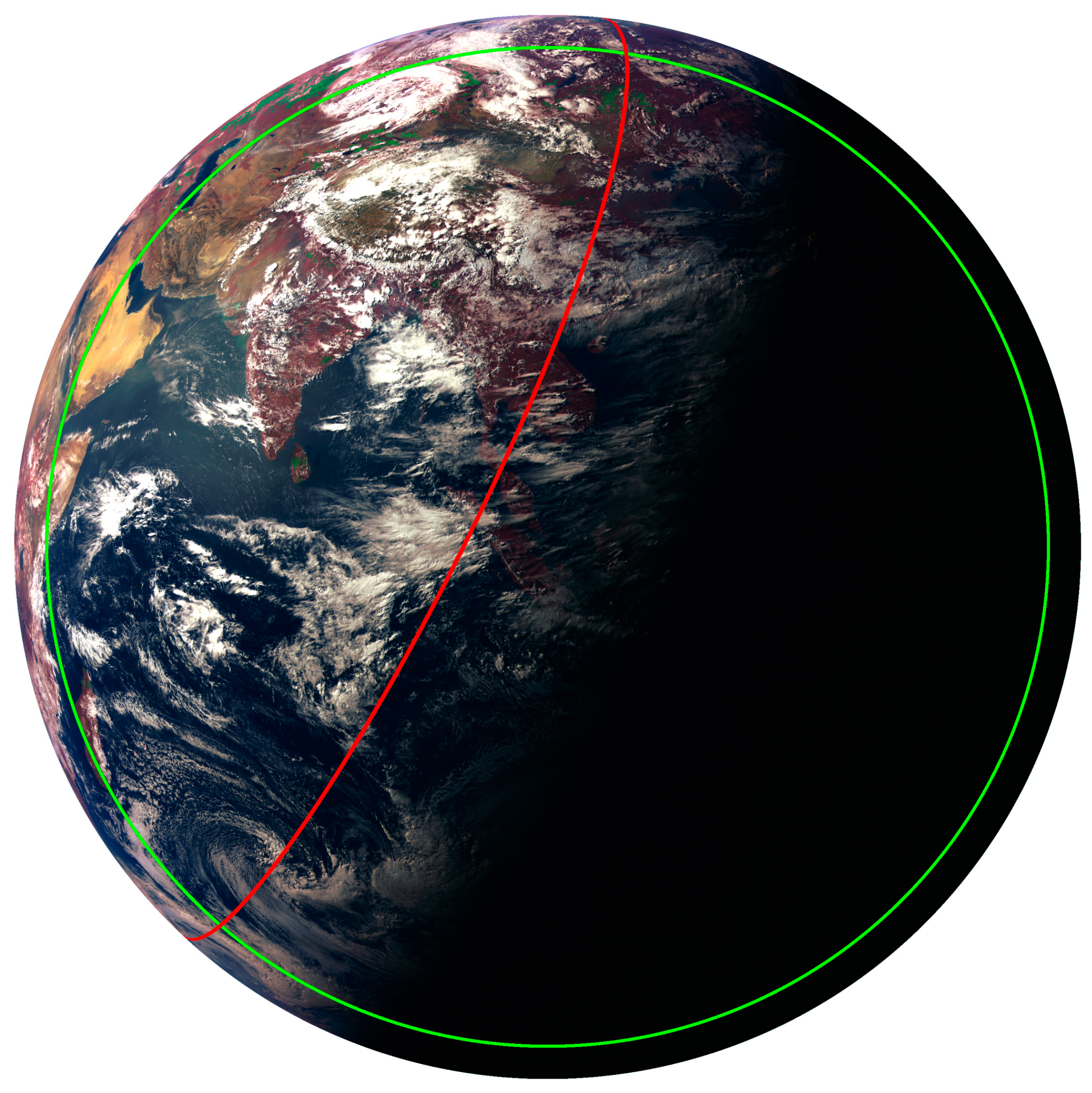
3.1.1. Division of Space Based on Satellite Zenith Angle

The baseline algorithm document formulated by NOAA stipulates that when the satellite zenith angle of a geostationary satellite is greater than 70°, the pixel is deemed invalid as a result of exceeding the satellite zenith angle range or quality degradation, no longer undergoing cloud mask judgment [9]. Now, with the development of machine learning methods and further development of deep learning methods, we hope to enable cloud mask measurement and improve its accuracy for every pixel captured by a geostationary satellite through deep learning methods. Therefore, in the following context, we train and discuss the parts with satellite zenith angles (SZAs) greater than 70° and less than 70° separately. Figure 2 shows the parts of FY-4A AGRI with SZAs greater than 70° and less than 70°.

3.1.2. Division of Daytime Based on Solar Zenith Angles

Since there is a significant difference in band selection schemes for daytime, nighttime, and twilight periods, cloud detection models need to be established separately for different time periods. The theoretical basis documents for the official cloud mask algorithms of ABI [9], SEVIRI [10], and AHI [48] all divide the daytime period based on solar zenith angle (Table 1). Combining the above division schemes and the characteristics of the AGRI satellite itself, a solar zenith angle < 70° is defined as daytime based on the solar zenith angle shown in Figure 2. The purpose of this paper is to develop a daytime cloud mask using deep learning techniques.

3.1.3. Four-Level Cloud Mask Division

Currently, most cloud mask algorithms, such as MODIS Terra/Aqua, GOES-R ABI, Himawari-8/9 AHI, and FY-4A AGRI, require a four-level (clear, probably clear, probably cloudy, or cloudy) result. The cloud mask model developed in this paper generates cloud probabilities ranging from 0 to 1. We divided the generated cloud mask probability results into four levels based on the ABI Enterprise Cloud Mask Algorithm (ECM) four-level classification threshold division scheme [19], and made some improvements on the basis of the original ABI ECM scheme. The output of the four-level cloud mask results enables downstream users to make modifications.

3.2. Data Preorocessing

We first need to preprocess the AGRI data. The AGRI data need to be geometrically corrected, and the 4km latitude/longitude lookup table provided by NSMC corresponds to the full-channel data of the full disk of the AGRI so that each point corresponds to the corresponding latitude/longitude. The data need to be radiometrically calibrated by converting the physically meaningless digital quantization values (DN) into physically meaningful reflectance (R) and brightness temperature (BT) values using the channel calibration lookup table provided by NSMC. Specifically, the DN values of the VIS and NIR channels are processed as R through the radiometric calibration lookup table of each channel, and the DN values of the rest of the infrared (IR) channels are processed as BT.
Next, to perform data preprocessing on the CALIPSO data, we used the number of clouds within each 1 km pixel (column) as determined by the number of layers found, and any CALIPSO columns with cloud counts exceeding 0 were categorized as cloudy, while the rest was categorized as clear.

3.3. Feature Selection

For daytime cloud detection, there are multiple band options available, including the VIS band, in addition to NIR, SWIR, MWIR, and LWIR bands. The official cloud mask algorithm theoretical basis documents of ABI [9], SEVIRI [10], and AHI [47] list the available daytime band options (Table 2). We chose seven bands ranging from 0.65 μm to 12.0 μm for deep learning daytime cloud detection. The selection was based on satellite sensor band choices and AGRI’s own band design. After data preprocessing, the study obtained R and BT values and calculated the Brightness Temperature Difference (BTD) between the two bands. The following eight feature values were chosen: R (0.65 μm), R (1.375 μm), R (1.61 μm), BT (10.7 μm), BTD (10.7–12.0 μm), BTD (8.5–12.0 μm), BTD (10.7–3.75 μm), and BTD (3.75–10.7 μm), composing the feature set defined as C .

3.4. Construction of the Datasets

3.4.1. Data Point Filtering Rules

The dataset was constructed using FY-4A AGRI 2021 data. Each CALIPSO pixel was matched with an AGRI pixel using the nearest-neighbor lookup method. Previous studies have used a time window of either 10 or 5 min for matching [9,31]. To enhance matching accuracy, this paper utilizes a 3 min time window. This means that data with a time difference greater than 3 min between a CALIPSO image element and an AGRI image element are excluded. Image elements with a latitude/longitude difference greater than 0.02° (for one AGRI pixel) are also excluded. The dataset that matches intercepts the data from the portion of the solar zenith angle that is less than 70° to create the daytime cloud mask dataset. The dataset is then divided in two based on SZA < 70° and SZA > 70°.
As one AGRI pixel corresponds to multiple CALIPSO pixels, a common preprocessing step when training imager cloud masks with CALIPSO observations is to filter the collocations using a variety of methods in order to infer when the CALIPSO cloud detections are unreliable or unrepresentative of the corresponding imager pixels. For instance, Heidinger et al. employed a filtering approach to AVHRR collocations, whereby only CALIPSO observations with a cloud fraction of either 0% or 100% along the 5 km trail were included [18]. Li et al. specified that horizontally inhomogeneous phase labels determined when the phase labels varied within five consecutive footprints were also discarded [30].
In accordance with the methodology proposed by Heidinger et al., all CALIPSO results with a cloud fraction not equal to 0.0 or 1.0 were excluded from the dataset. This was done to ensure the finer spatial scale 1 km CALIPSO data were applied to the coarser spatial scale 4 km high-resolution AGRI image elements [18,19].

3.4.2. Data Block Establishment Rules

Although the cloud mask is the output of each image element, cloud detection accuracy based on a single point is limited. Therefore, it is necessary to use surrounding pixel points to assist in judgment during the training process [19]. We take the matched point as the center point, select the surrounding 9 × 9 size range, and intercept the set of eight feature channels ( C ) to form a data block ( X 8 × 9 × 9 ) as input data. To ensure that each feature has a balanced impact on the model, we need to remove the difference in magnitude between different channels. Therefore, we normalized the data by scaling it to a range of 0 to 1 using the maximum–minimum value normalization formula shown below:
x ^ i j k = x i j k m i n ( x k ) m a x ( x k ) m i n ( x k ) ,
where x i j k represents each pixel on each channel ( i [ 0 , 9 ) , j [ 0 , 9 ) , k [ 0 , 8 ) ) and x k represents the data for channel k in the data block, with m i n ( x k ) and m a x ( x k ) representing the minimum and maximum values of all the data for channel k in the established dataset, respectively.
We divided the two datasets (SZA < 70° and SZA > 70°) after preprocessing (70% into the training set and 30% into the test set); the SZA < 70° dataset has a total of 358,300 samples, of which 253,800 are for the training set and 104,500 are for the test set, and the SZA > 70° dataset has a total of 17,000 samples, of which 12,600 are for the training set and 4400 are for the test set.

3.5. The CACM-Net Architecture

This section introduces the deep learning algorithms proposed and applied in this research. It outlines the network architecture, training, and implementation process to present the reasons for the model architecture and reveal the underlying mechanisms and roles played by each module. This paper presents the construction of a Convolutional Attention Cloud Mask Network (CACM-Net) for the AGRI cloud detection task. CACM-Net combines the convolution module and the attention module to improve the accuracy of cloud detection. The network is divided into two steps, namely the training step and the prediction step, as shown in Figure 3.

3.5.1. Training Step

Judging whether an image element contains clouds is highly correlated with the data in its surrounding area. The distribution of clouds is localized, and the convolution operation is a localization operation whose computation results depend on the local information in the input data. The convolution operation extracts localized features from the input data by sliding a small, learnable filter (also known as a convolution kernel or a weight) over the input data. This operation effectively utilizes the pixel points around the image element to be judged and extracts deeper features. The FY-4A AGRI cloud detection deep learning model is constructed based on the convolutional module. A pooling layer is added on top of the convolutional layer to reduce data dimensionality, improve network robustness, and prevent data overfitting to some extent. The maximum pooling layer is used in this paper to extract the maximum value of local feature blocks in the feature map [48]. To enable the neural network to have a nonlinear fitting ability, a nonlinear activation function needs to be introduced. The Rectified Linear Unit (ReLU) function is a commonly used activation function. Its formula is shown in (2). The function outputs its own value when it receives a positive input and outputs 0 when it receives a negative value [49]. This activation function is simple and has good learning efficiency.
R e L U ( x ) = m a x ( x , 0 )
For the cloud detection task, it is necessary to have a mechanism to fuse information between channels. This is because the information from multiple channels is inter-related and influential, and there are differences in the spatial dimensions of the influence of each region on the centroid. Therefore, weighted fusion of data in the spatial dimensions are required. Therefore, we incorporated the Convolutional Block Attention Module (CBAM Block) proposed by Woo et al. [50]. CBAM is a simple and effective feed-forward convolutional neural network attention module. The module consists of a channel attention submodule and a spatial attention submodule, as shown in Figure 4. The channel attention submodule creates a channel attention graph by utilizing the relationship between the information of different bands. This submodule assigns different weights according to the degree of correlation of different bands, effectively aggregating the information of each band. The spatial attention submodule generates a spatial attention map by utilizing the spatial relationship between different locations of individual bands. This complements the lack of spatial feature fusion capability of channel attention. Specifically, the single data block ( X 9 × 9 × 8 ) created above is fed into the CBAM block, and the input features are passed through the channel attention module and spatial attention module to obtain refined features with the same shape as the original data but with more distinctive features, which are then fed into the subsequent convolution module.
The established data block (X) is input into the attention module. The output feature map undergoes multiple convolution, activation, and maximum pooling operations to extract data features. This fuses information captured in different spatial scales and channels. Finally, the feature map is spread out and fed into the fully connected binary classification network to obtain the classification results of the data block as cloudy or clear.

3.5.2. Prediction Step

In the training step, we input the created data block (X) into CACM-Net according to SZA < 70° and SZA > 70°, respectively, and save the CACM-Net (SZA < 70°) model and the CACM-Net (SZA > 70°) model. In the prediction step, we pass the raw FY-4A AGRI level-1 data into the CACM-Net preprocessing flow, and after radiometric calibration and band selection, we divide the full-disk data according to SZA < 70° and SZA > 70° and input them into the cloud mask models of CACM-Net (SZA < 70°) and CACM-Net (SZA > 70°), respectively. The results are then distributed in the 0–1 range for both cloudy and clear results using the softmax function with appropriate thresholds; then, the two data are stitched together to form a complete AGRI cloud mask prediction.

3.5.3. Implementation Details

CACM-Net was implemented using CUDA version 11.8 and the Pytorch framework 2.0.1. For better model generalization, we used a dropout of 0.5. Dropout is a method of randomly setting the output of a neuron to zero [51], and when configuring CACM-Net during training, the loss was calculated using the cross-entropy loss function and optimized using the Adam optimizer [52]. The value of α was 0.9, and the value of β was 0.99. The gradient of the parameters that can be learned in the network was computed by the backpropagation algorithm [53], the initial learning rate was set to 0.01, and a ReduceLROnPlateau learning rate update strategy was adopted. During the training process, if after 30 epochs, test set accuracy was still not improved the training was ended early, with a batch size of 256.

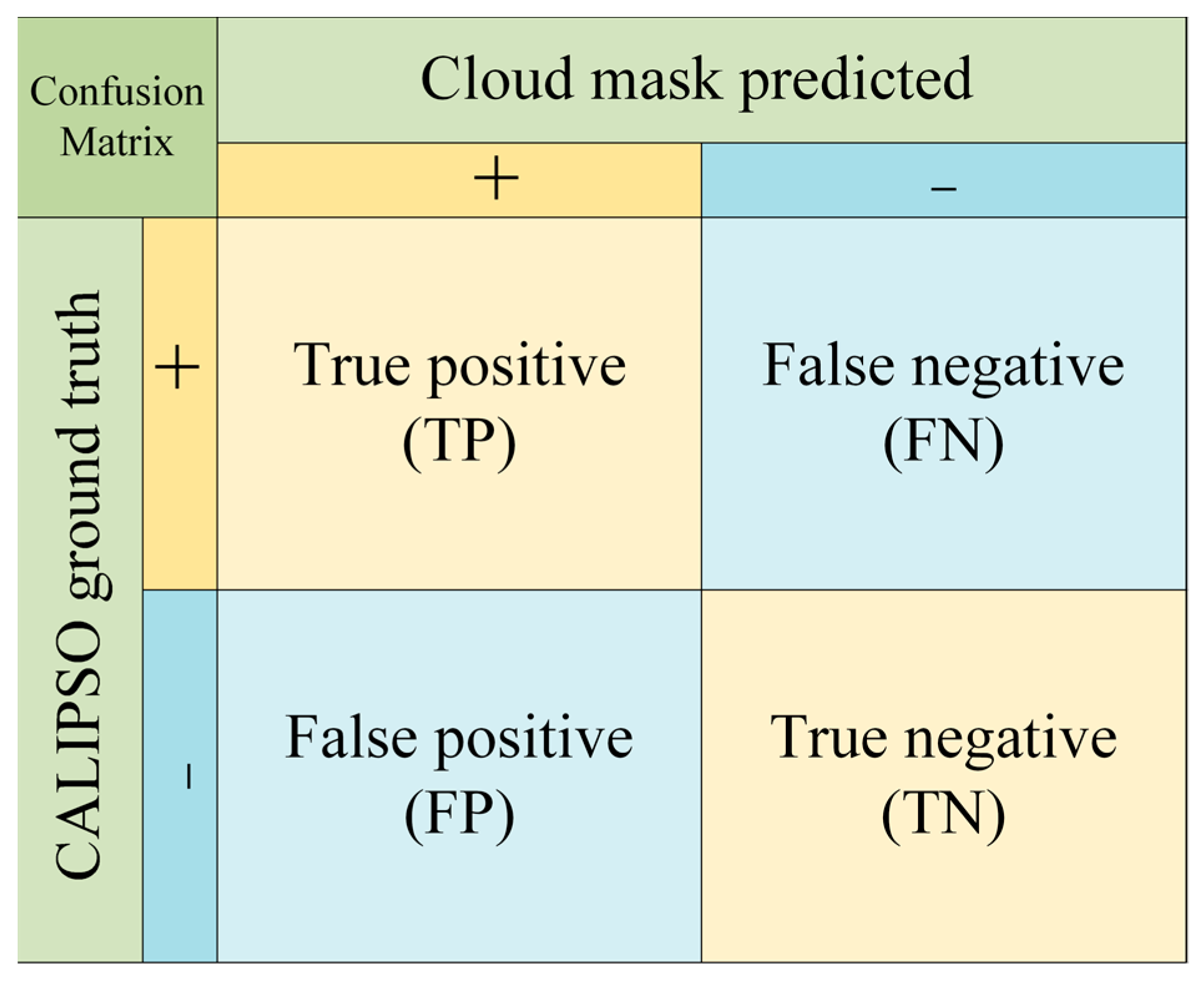
3.6. Metric Definitions

3.6.1. Evaluation Metrics

In order to evaluate the predictive ability of the cloud mask model, the truth values detected by CALIPSO are compared with the results predicted by the model (clear and probably clear as clear and cloud and probably cloudy as cloudy), transforming them into a binary classification and introducing the following metrics for evaluation. The basis for calculating the evaluation metrics can be obtained from the confusion matrix shown in Figure 5, from which it can be seen that the image elements recognized by the algorithm as cloud and clear and by CALIPSO as cloud are true positive (TP) and false negative (FN), respectively, and the image elements recognized by the algorithm as clear and cloud and by CALIPSO as clear are true negative (TN) and false positive (FP), respectively. In addition, accuracy, recall (POD), precision, F1 score (F1), and false alarm ratio (FAR) are calculated as follows:
accuracy = TP + TN TP + FN + FP + TN
POD = TP TP + FN
Precision = TP TP + FP
F 1 = 2 Precision POD Precision + POD
FAR = FP FP + TP
Accuracy refers to the proportion of correctly predicted samples to the total number of samples. High accuracy indicates that the model has strong overall prediction ability. POD, also known as recall, indicates whether the model comprehensively covers the real cloudy situation. The best performance is achieved when the value is 1, and the worst performance is achieved when the value is 0. Precision is the ratio of correctly predicted clouds to the total number of predicted clouds, measuring the accuracy of the model in predicting positive instances. To account for biases in the above metrics, the F1 score combines precision and POD, resulting in the reconciled average of precision and recall. This reflects the overall performance of the model. To evaluate the possible misdetection rate of the model, we introduce FAR. The closer FAR is to 0, the better the model’s performance.

3.6.2. Cross-Comparison Metrics

We define the deviation (ΔS) of the CACM-Net results from the operationalized cloud mask and count its consistency and offset, which is defined by the following formula:
Δ S = S C A C M N e t S c l o u d   m a s k   p r o d u c t
where S C A C M N e t and S c l o u d   m a s k   p r o d u c t are the cloudy and clear classification results used to define the CACM-Net cloud mask and the operational satellite sensor cloud mask, respectively. We transformed the four classified cloud mask results (clear = 0; probably clear = 1; probably cloudy2; cloudy = 3) into two classified results (clear = 0; cloudy = 1) and statistically analyzed them. The range of their deviations is [ 1 ,   1 ] , where 0 indicates that CACM-Net has no deviation from the operational cloud mask product judgments and −1 and 1 indicate their tendency to be clear and their tendency to be cloudy, respectively. For the purpose of the subsequent analysis, we define the following three types.
Δ S = 0 , n o   s h i f t
Δ S = 1 , c l e a r   s h i f t
Δ S = 1 , c l o u d y   s h i f t

4. Results

4.1. CACM-Net Cloud Mask Results

Since geostationary satellites have large aberrations in the region of SZA > 70°, which may lead to a large discrepancy between the mapping of satellite data and cloud distributions, we utilized the already established training dataset for the whole year of 2021 to train two models for the region of SZA < 70° and the region of SZA > 70°, respectively, namely CACM-Net (SZA < 70°) and CACM-Net (SZA > 70°). The evaluation results of their test sets are shown in Table 3. For CACM-Net (SZA < 70°), the four-level cloud mask thresholds are determined based on the probability density curves as 0.09, 0.56, and 0.87, resulting in an accuracy of 92.2%, indicating high precision. For CACM-Net (SZA > 70°), the four-level cloud mask thresholds are 0.02, 0.52, and 0.89 based on probability density curves. The model’s accuracy in this region decreases compared to that in the part of SZA < 70° due to the fewer number of available data for training and a decrease in data quality at level 1.
Monthly analysis is conducted on the accuracy trend for CACM-Net (SZA < 70°) and CACM-Net (SZA > 70°) in Figure 6a. The results show that CACM-Net (SZA < 70°) is consistently stable throughout 2021 and exhibits higher detection accuracy during the summer season. On the other hand, the model accuracy of CACM-Net (SZA > 70°) fluctuates significantly, but its overall performance remains stable.

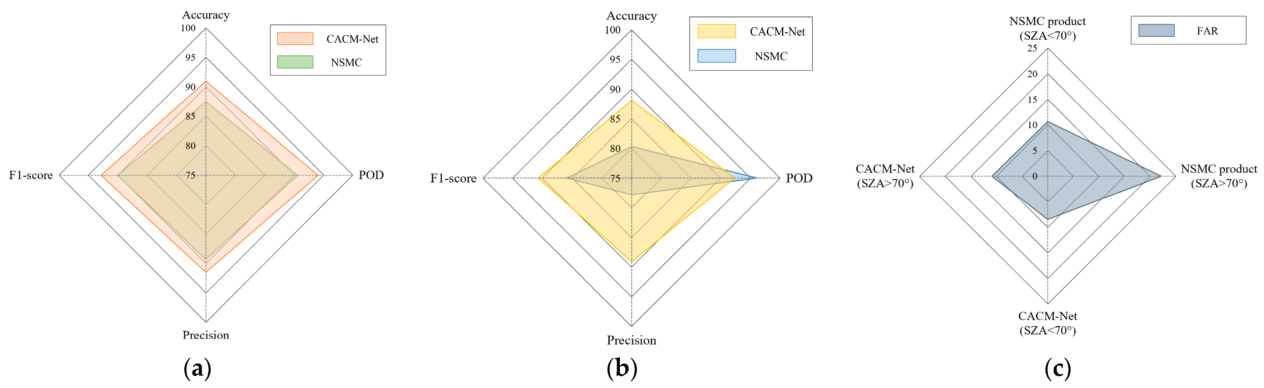
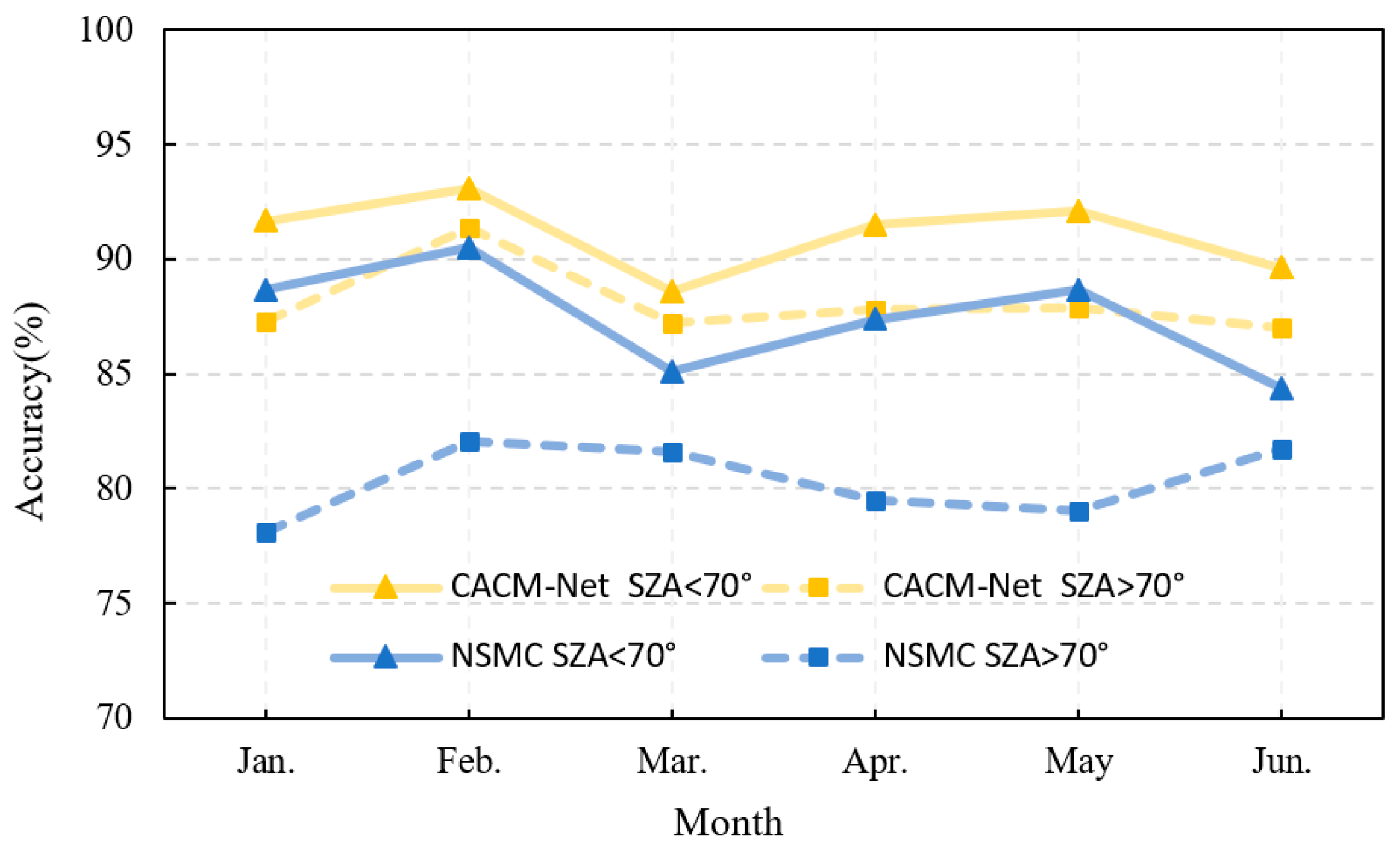
4.2. Evaluation Results of NSMC Cloud Mask Products

This section introduces the CALIPSO data as the truth value to evaluate the accuracy of NSMC’s cloud mask product. The CALIPSO and AGRI level-1 data for the entire year of 2021 were strictly matched using the algorithm described in Section 3.3 of this paper. The resulting matched data were then evaluated against the image elements of NSMC’s cloud mask product using the evaluation indices outlined in Section 3.5. Table 3 shows that the NSMC AGRI cloud mask products have higher POD values and corresponding higher FAR values in the SZA < 70° and SZA > 70° sections. This suggests that the cloud detection algorithms tend to categorize more pixel points as clouds, which has been previously confirmed by scholars. This may be due to the overestimation of the number of cloud pixels as a result of the EMISS4 test [40]. Additionally, the accuracy of the cloud mask is lower for SZA values greater than 70° compared to those less than 70°.
Similarly, a monthly analysis of the accuracy for NSMC cloud mask products in 2021 was conducted (see Figure 6b). It was found that the accuracies in February and March were significantly lower than in other months for SZA < 70° and SZA > 70°. A day-by-day accuracy analysis was conducted, revealing that the NSMC cloud mask products may have experienced daytime cloud mask algorithm failure during the periods of February 18–22 and 27 and March 1–8. During these time periods, most of the pixels were incorrectly judged as clouds, resulting in low average cloud mask accuracy for February and March.

5. Discussion

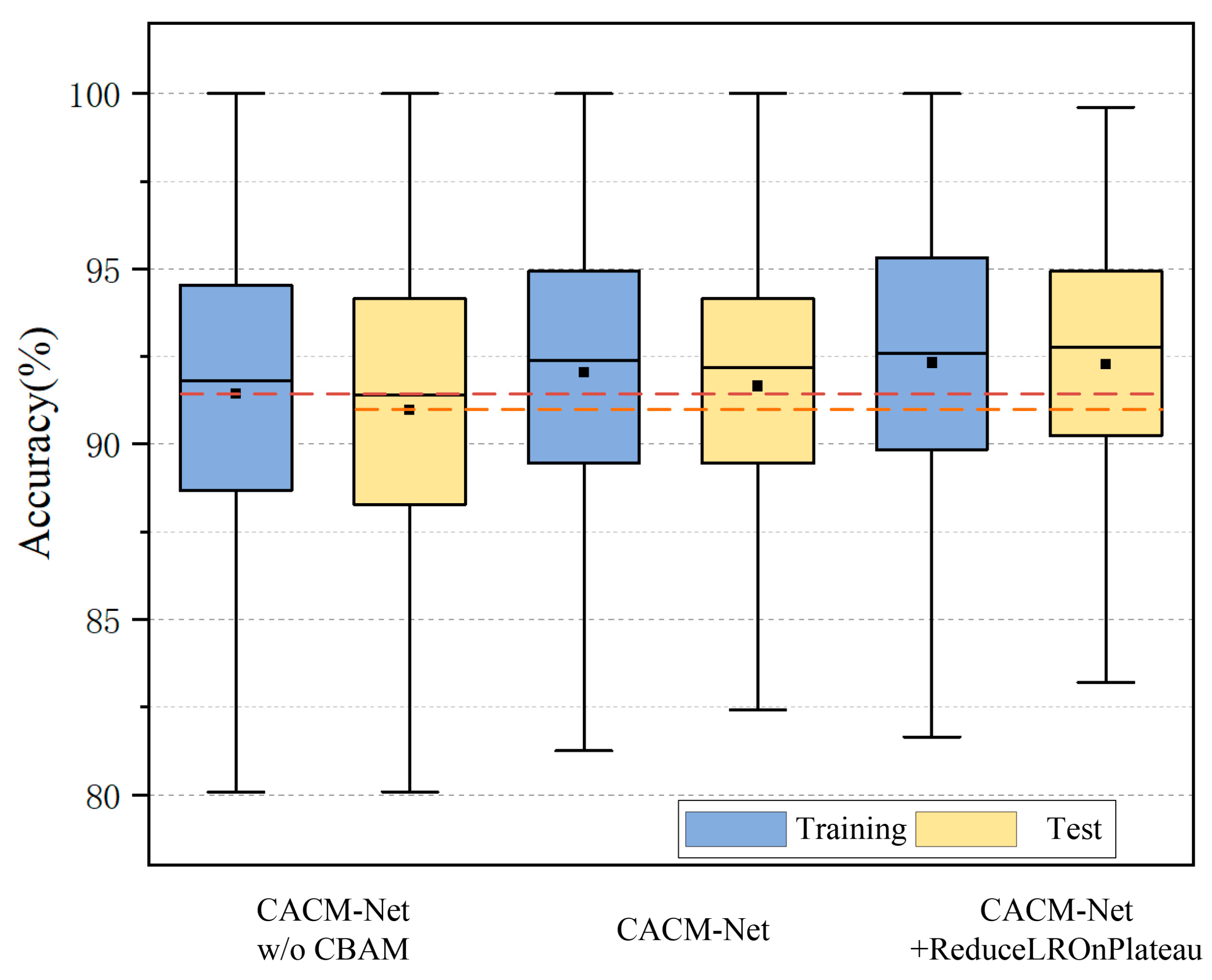
5.1. Ablation Experiments and Training Strategy

To demonstrate the effectiveness of adding the attention module before the convolution module, we conducted ablation experiments. Specifically, we removed the CBAM module to observe any changes in the final cloud mask’s impact. Taking the data in the SZA < 70° part as an example, we recorded the accuracy rate of each batch in the training and validation sets for the last epoch. Box plots were drawn to show the effect of the CBAM module, and the results are presented in Figure 7. The CBAM module was removed for training, and compared to the model without the CBAM module, the addition of the CBAM module improved all aspects of the network’s performance. Specifically, on the test set, the accuracy improved by 0.8%. As can be seen in Table 4, the addition of the CBAM module improved POD by 0.1%, precision by 1%, and F1 score by 0.5%. This indicates an increase in the accuracy of the model, allowing it to detect more cloud image elements while reducing the error rate, resulting in a more robust model. To enhance the model’s accuracy, we incorporated the ReduceLROnPlateau learning rate updating strategy during training. This resulted in a 0.5% improvement in test accuracy, a 0.15% improvement in POD, and a 0.6% improvement in F1 score. Although the model’s FAR increased slightly, its overall performance improved significantly, and it demonstrated stable performance on both the training and test sets.

5.2. Four-Level Cloud Mask Division

Since cloud mask products from most satellites usually provide four cloud classifications (clear, probably clear, probably cloudy, and cloudy), most studies classify cloud masks into the four categories based on the confidence level. The cutoff between clear and cloudy is usually set to 0.5, while the cutoffs between probably clear and probably cloudy are set to 0.1 and 0.9, respectively [18,20]. However, this approach lacks objectivity in choosing appropriate thresholds for trained data and constructed models. Therefore, we propose a classification scheme that objectively distinguishes between the four classes of cases. Figure 8 displays the cloud probability distribution curve for a daytime scene with SZA < 70° generated from the training set of CACM-Net. To distinguish between clear and cloudy pixels, we use the minimum value of this curve, which is 0.56, as the initial threshold. To distinguish between cloudy and probably cloudy pixels and clear and probably clear pixels, we calculate the second-order derivative of the curve and determine the descending and ascending intersections of the first second-order derivative, which are 0.09 and 0.87, respectively. We use a threshold value of 0.87 for cloudy and probably cloudy pixels and a threshold value of 0.09 for clear and probably clear pixels. By utilizing this method, we can obtain a reasonable segmentation scheme for the various models that have been trained. Downstream users can modify the threshold value according to their usage scenario. We evaluated CACM-Net using thresholds of 0.1, 0.5, and 0.9 for two different SZAs. Compared to the above threshold selection scheme, the results in Table 5 demonstrate that the model performances were improved to some extent.

5.3. The Need for SZA Demarcation

In order to verify that the large difference in the mapping relationship between AGRI L1 data and cloud distributions for SZA < 70° and SZA > 70° causes the two parts of the data to interact with each other, resulting in “contamination” of the training dataset and, thus, lowering the accuracy of the model, we set up a model without distinguishing between the SZAs, namely CACM-Net (Full), and set the four-level cloud mask thresholds of 0.05, 0.52, and 0.83 based on the probability density curve to obtain the final model results. The results (Figure 9) show that the accuracy of the model without dividing the SZA is reduced to varying degrees compared to both the SZA < 70° and SZA > 70° models; specifically, the accuracy is reduced by 3.3%, the F1 score is reduced by 2.4%, and the FAR is elevated by 7.3% compared to the SZA < 70° model, and the FAR is elevated by 7.3% compared to the SZA > 70° model. Since not making the SZA distinction increases the POD and FAR, training the model without SZA division may cause the model to classify more pixels as clouds overall, resulting in lower model accuracy and worse performance.
We compared the results of the 2021 CACM-Net cloud mask on the test dataset with the evaluation results of the NSMC cloud mask product in both the SZA < 70° and SZA > 70° regions of performance.
In the region where SZA < 70°, CACM-Net outperforms the NSMC cloud mask product. Its accuracy, precision, and F1 score are significantly improved compared to the NSMC cloud mask product by 4.8%, 7.3%, and 3.6%, respectively. Additionally, the FAR decreases by about 7.3%, which partially addresses the issue of the NSMC product’s tendency to overestimate the amount of cloud. This improvement enhances the accuracy of the cloud mask. We randomly selected the FY-4A AGRI data at 5:00 UTC on 21 April 2021, the moment without model training, for demonstration (Figure 10), and in the part of SZA < 70°, referring to the reflectance map of 0.65 μm, when comparing the cloud mask results obtained by CACM-Net and NSMC, it is evident that CACM-Net provides more detailed information. Specifically, CACM-Net is able to identify some pixels that the NSMC cloud mask classified as cloudy as clear. This improvement is particularly noticeable in the circled area of the figure, and it helps to address the issue of the NSMC cloud mask overestimating the number of cloudy pixels, thereby enhancing the accuracy of the cloud mask.
In the section where SZA > 70°, CACM-Net outperforms the NSMC cloud mask product in terms of accuracy, precision, and F1 score by 12.2%, 19.5%, and 8%, respectively. Additionally, the FAR decreases by about 19.5%. Specifically, in Figure 10, the area marked by the circle shows that CACM-Net can detect the cloud-free area and provide more details, thereby improving the quality of the cloud mask and addressing the issues with the NSMC cloud mask. Training the model individually against different SZA regions can improve its accuracy.

5.4. Validation and Cross-Comparison

5.4.1. Validation

To validate the performance, generalization, and stability of the model runs of CACM-Net, we evaluated it on data from January–June 2023 for operational running and compared it with NSMC’s cloud mask product. The independent validation dataset was built for January–June 2023 using the matching scheme described in Section 3.4. The dataset was completely independent from the network and served as a validation dataset. Both CACM-Net (SZA < 70°) and CACM-Net (SZA > 70°) showed a decrease in accuracy on the new test set, with accuracy dropping from 92.2% to 91.0% and from 89.7% to 88.1%, respectively. The precision rate and F1 score both decreased to 88.1% respectively. However, they were still within an acceptable range, indicating that the CACM-Net model has good stability and generalizability and can perform well on independent validation sets.
The NSMC cloud mask product was compared with CACM-Net for the given time period, and the results (Figure 11) indicate that CACM-Net outperforms NSMC’s cloud mask in terms of accuracy and model stability. Specifically, the accuracy of CACM-Net is improved by 3.5%, POD by 3.5%, precision by 2.2%, F1 score by 2.8%, and FAR by 2.2% compared to NSMC’s cloud mask product in the SZA < 70° part. In the SZA > 70° part, the accuracy of CACM-Net is improved by 7.8%, precision by 11.3%, and F1 score by 4.8%, while POD is reduced by 3.8% and FAR is reduced by 11.3%. We conducted a further analysis of the performance of CACM-Net and the NSMC cloud mask product for each month from January to June of 2023 (Figure 12). The results of this analysis demonstrate that, in all respects, CACM-Net outperforms the NSMC cloud mask product and displays greater stability of performance on a monthly basis.

5.4.2. Case Demonstration

The CACM-Net model was employed to illustrate the progression of Typhoon Nanmadol from its genesis to dissipation between 13 and 20 September 2022 [54,55]. Figure 13 shows a true-color plot of typhoon arising on 13 September 2022, peaking on 16 September 2022, and denaturing on 20 September 2022 (Table 6), and its corresponding CACM-Net cloud mask results. (Table 6). It can be observed that the CACM-Net model demonstrates superior performance in detecting the complete process of typhoon change. This evidence supports the assertion that the model developed in this study has significant practical application value.

5.4.3. Cross-Comparison

To validate the consistency of CACM-Net’s cloud mask results with other operational cloud mask products, we assessed the consistency of its satellite SZA < 70° portion with MODSI’s and Himawari-9’s cloud mask products using the metrics defined in Section 3.5.2.
The 5 km cloud mask products of the MODIS Terra MOD series for 12 time periods from January to June 2023 were selected and matched with AGRI 4 km latitude/longitude geographic data for nearest-neighbor matching. The time window was controlled to 5 min to ensure the accuracy of consistency assessment. The matched pixel points and the assessment results are shown in Table 7. The results indicate that the cloud mask consistencies of CACM-Net and MODIS are good, reaching 88%. CACM-Net tends to classify more pixels as clouds compared to MODIS cloud mask products, resulting in a cloudy shift of 6.9%. The data selected for display in Figure 14a–d are from 16 January 2023 at 1:00 UTC. The figure indicates improved consistency and a tendency to classify more pixels as clouds.
For the Himawari-9 AHI, we selected 5 km cloud mask products for 12 time periods from January to June 2023. We matched them with 4 km latitude/longitude data from AGRI and controlled the time within 3 min to obtain more accurate evaluation results. These results are shown in Table 7. The agreement between the two reaches 86.3%. Compared to the Himawari-9 cloud mask product, CACM-Net tends to determine more image elements as clear, and its clear shift reaches 7.6%. The cloud mask results of the AHI cloud mask over CACM-Net at 4:00 UTC time on 1 January 2023 were selected for presentation in Figure 14e–h. The results show better consistency, but there may be leakage in the eastern part of Australia, and the discrepancy between the two is consistent with the statistical results.

6. Conclusions

This paper proposes a CACM-Net model based on deep learning for the development of a daytime cloud mask algorithm for the AGRI sensor onboard the FY-4A satellite.
The training dataset is a crucial component in establishing deep learning models. For the observation mode of geostationary satellites, we used the 2021 CALIPSO data as the true value and matched it with the FY-4A AGRI image elements to establish the training dataset. Daytime was specified as a solar zenith angle of less than 70°, with a time window of 3 min and a spatial window of 0.02°. Based on SZA < 70° and SZA > 70°, we selected eight features consisting of radiance, bright temperature value, and bright temperature difference in seven bands (0.65, 1.375, 1.61, 3.75, 8.5, 10.7, and 12.0 μm) to construct the training dataset for the CACM-Net cloud mask model. The strict matching scheme used in this study provides strong support for the construction of the deep learning model.
The CACM-Net was constructed by adding an attention mechanism to the convolutional neural network based on the constructed training dataset. The accuracy of CACM-Net was evaluated using the test dataset. The NSMC’s official cloud mask results were also evaluated using the same matching method and compared with the CACM-Net model built in this paper. The results indicate that the NSMC cloud mask product tends to overestimate the amount of cloud, which is consistent with previous studies. Additionally, lower accuracy was observed in the SZA > 70° part. When comparing the results of the CACM-Net cloud mask established in this paper with the evaluation results of the NSMC cloud mask product, the accuracy, precision, and F1 score in the SZA < 70° part improved by 4.8%, 7.3%, and 3.6%, respectively, compared to NSMC’s cloud mask product. Additionally, the FAR decreased by about 7.3%. In the SZA > 70° part, the performance of the CACM-Net cloud mask product also improved by 4.8%, 7.3%, and 3.6%, respectively. CACM-Net outperforms the NSMC cloud mask product, improvements in accuracy, precision, and F1 score of 12.2%, 19.5%, and 8%, respectively. Additionally, its FAR decreased by approximately 19.5% compared to the NSMC cloud mask product. To some extent, we have addressed the issue of NSMC cloud mask products overestimating cloud amounts and improved the accuracy of cloud masks. We also developed CACM-Net (Full) without distinguishing SZA, resulting in lower accuracy compared to the model built separately based on SZA. This proves that building CACM-Net (SZA < 70°) and the CACM-Net (SZA > 70°) separately is effective for improving the model’s accuracy. By dividing SZA and training the cloud mask model separately, not only improved the accuracy of the cloud mask for SZA < 70° but also fully utilized SZA > 70° to build a more accurate cloud mask model that outperforms existing NSMC cloud mask products.
To verify the generalization and stability of the CACM-Net model, we used CALIPSO data from January to June 2023 as the true value. We built a set of independent validation datasets using the same method and examined the running results. We compared the results with the official products of NSMC and found that the CACM-Net cloud mask model exhibits a decrease in accuracy on this dataset, but it falls within the acceptable range. In comparison to the NSMC cloud mask product, the model presented in this paper demonstrates better overall performance. Specifically, for SZA < 70°, the accuracy improves by 3.5%, precision by 2.2%, and F1 score by 2.8%, and FAR is reduced by 2%. In the SZA > 70° portion, the accuracy improves by 7.8%, precision improves by 11.3%, and the F1 score improves by 4.8%. Upon analyzing the monthly trend of accuracy, it is evident that the performance of CACM-Net is consistently stable and exhibits higher accuracy. Therefore, the cloud mask model proposed in this paper is more stable and accurate.
Meanwhile, we cross-compared the results with other mainstream satellite cloud mask products. The CACM-Net cloud mask results showed 88.6% consistency with MODIS cloud mask products and 86.3% consistency with Himawari-9 cloud mask products, indicating a high level of consistency. This paper establishes the CACM-Net cloud mask deep learning model, which produces high-quality cloud mask products with better accuracy than existing NSMC cloud mask products. The model can also be applied to cloud mask algorithms for other satellite sensors.
CACM-Net was built using only data with cloud fractions of 0 and 1, which means that the model did not learn the features of the transition image elements in between. Subsequently, we plan to consider feeding this part of the data into the model to determine the appropriate segmentation scheme.
Our future work will concentrate on developing deep learning models for a nighttime cloud mask algorithm for FY-4A AGRI.

Author Contributions

Conceptualization, Z.Q. and D.Z.; Methodology, J.Y., B.S., J.L. and Y.W.; Validation, J.Y.; Formal analysis, J.Y.; Data curation, J.Y.; Writing—original draft, J.Y.; Writing—review & editing, Z.Q. and D.Z.; Funding acquisition, K.L. (Kuo Liao) and K.L. (Kailin Li). All authors have read and agreed to the published version of the manuscript.

Funding

This research was funded by [East China Collaborative Innovation Fund for Meteorological Science and Technology] grant number [QYHZ202110] and [Advanced Program for FY Satellite Applications 2022] grant number [FY-APP-2022.0610]

Conflicts of Interest

The authors declare no conflict of interest.

References

  1. Zhu, Z.; Woodcock, C.E. Automated cloud, cloud shadow, and snow detection in multitemporal Landsat data: An algorithm designed specifically for monitoring land cover change. Remote Sens. Environ. 2014, 152, 217–234. [Google Scholar] [CrossRef]
  2. Zhang, Y.; Rossow, W.B.; Lacis, A.A.; Oinas, V.; Mishchenko, M.I. Calculation of radiative fluxes from the surface to top of atmosphere based on ISCCP and other global data sets: Refinements of the radiative transfer model and the input data. J. Geophys. Res. Atmos. 2004, 109. [Google Scholar] [CrossRef]
  3. Stubenrauch, C.J.; Rossow, W.B.; Kinne, S.; Ackerman, S.; Cesana, G.; Chepfer, H.; Di Girolamo, L.; Getzewich, B.; Guignard, A.; Heidinger, A. Assessment of global cloud datasets from satellites: Project and database initiated by the GEWEX radiation panel. Bull. Am. Meteorol. Soc. 2013, 94, 1031–1049. [Google Scholar] [CrossRef]
  4. Stowe, L.L.; Davis, P.A.; McClain, E.P. Scientific basis and initial evaluation of the CLAVR-1 global clear/cloud classification algorithm for the Advanced Very High Resolution Radiometer. J. Atmos. Ocean. Technol. 1999, 16, 656–681. [Google Scholar] [CrossRef]
  5. Ackerman, S.; Frey, R.; Strabala, K.; Liu, Y.; Gumley, L.; Baum, B. Discriminating Clear-Sky from Cloud with MODIS Algorithm Theoretical Basis Document (MOD35); Institute for Meteorological Satellite Studies, University of Wisconsin: Madison, WI, USA, 2010. [Google Scholar]
  6. Hutchison, K.D.; Roskovensky, J.K.; Jackson, J.M.; Heidinger, A.K.; Kopp, T.J.; Pavolonis, M.J.; Frey, R. Automated cloud detection and classification of data collected by the Visible Infrared Imager Radiometer Suite (VIIRS). Int. J. Remote Sens. 2005, 26, 4681–4706. [Google Scholar] [CrossRef]
  7. Kopp, T.J.; Thomas, W.; Heidinger, A.K.; Botambekov, D.; Frey, R.A.; Hutchison, K.D.; Iisager, B.D.; Brueske, K.; Reed, B. The VIIRS Cloud Mask: Progress in the first year of S-NPP toward a common cloud detection scheme. J. Geophys. Res. Atmos. 2014, 119, 2441–2456. [Google Scholar] [CrossRef]
  8. Frey, R.A.; Ackerman, S.A.; Holz, R.E.; Dutcher, S.; Griffith, Z. The Continuity MODIS-VIIRS Cloud Mask. Remote Sens. 2020, 12, 3334. [Google Scholar] [CrossRef]
  9. Heidinger, A.; Straka III, W.C. Algorithm Theoretical Basis Doucment: ABI Cloud Mask; NOAA/NESDIS Center for Satellite Applications and Research: Silver Spring, ML, USA, 2012. [Google Scholar]
  10. Le GLeau, H. Algorithm Theoretical Basis Document for the Cloud Product Processors of the NWC/GEO; Technical Report, EUMETSAT NWC SAF Support to Nowcasting And Very Short Range Forecasting, Centre de Meteorologie Spatiale: Meteo, France, 2019. [Google Scholar]
  11. Miller, S.D.; Noh, Y.-J.; Heidinger, A.K. Liquid-top mixed-phase cloud detection from shortwave-infrared satellite radiometer observations: A physical basis. J. Geophys. Res. Atmos. 2014, 119, 8245–8267. [Google Scholar] [CrossRef]
  12. Pavolonis, M.J.; Heidinger, A.K. Daytime cloud overlap detection from AVHRR and VIIRS. J. Appl. Meteorol. Climatol. 2004, 43, 762–778. [Google Scholar] [CrossRef]
  13. Meister, G.; Franz, B.A.; Kwiatkowska, E.J.; McClain, C.R. Corrections to the calibration of MODIS Aqua ocean color bands derived from SeaWiFS data. IEEE Trans. Geosci. Remote Sens. 2011, 50, 310–319. [Google Scholar] [CrossRef]
  14. Stubenrauch, C.; Cros, S.; Guignard, A.; Lamquin, N. A 6-year global cloud climatology from the Atmospheric InfraRed Sounder AIRS and a statistical analysis in synergy with CALIPSO and CloudSat. Atmos. Chem. Phys. 2010, 10, 7197–7214. [Google Scholar] [CrossRef]
  15. Addesso, P.; Conte, R.; Longo, M.; Restaino, R.; Vivone, G. SVM-based cloud detection aided by contextual information. In Proceedings of the 2012 Tyrrhenian Workshop on Advances in Radar and Remote Sensing (TyWRRS), Naples, Italy, 12–14 September 2012; pp. 214–221. [Google Scholar]
  16. Reguiegue, M.; Chouireb, F. Automatic day time cloud detection over land and sea from MSG SEVIRI images using three features and two artificial intelligence approaches. Signal Image Video Process. 2017, 12, 189–196. [Google Scholar] [CrossRef]
  17. Wang, C.; Platnick, S.; Meyer, K.; Zhang, Z.; Zhou, Y. A machine-learning-based cloud detection and thermodynamic-phase classification algorithm using passive spectral observations. Atmos. Meas. Tech. 2020, 13, 2257–2277. [Google Scholar] [CrossRef]
  18. Heidinger, A.K.; Evan, A.T.; Foster, M.J.; Walther, A. A Naive Bayesian Cloud-Detection Scheme Derived from CALIPSO and Applied within PATMOS-x. J. Appl. Meteorol. Climatol. 2012, 51, 1129–1144. [Google Scholar] [CrossRef]
  19. Heidinger, A.; Botambekov, D.; Walther, A. A Naïve Bayesian Cloud Mask Delivered to NOAA Enterprise. Algorithm Theoretical Basis Document. 2016. Available online: https://www.star.nesdis.noaa.gov/goesr/documents/ATBDs/Enterprise/ATBD_Enterprise_Cloud_Mask_v1.2_2020_10_01.pdf (accessed on 1 April 2023).
  20. Haynes, J.M.; Noh, Y.-J.; Miller, S.D.; Haynes, K.D.; Ebert-Uphoff, I.; Heidinger, A. Low cloud detection in multilayer scenes using satellite imagery with machine learning methods. J. Atmos. Ocean. Technol. 2022, 39, 319–334. [Google Scholar] [CrossRef]
  21. Ganci, G.; Vicari, A.; Bonfiglio, S.; Gallo, G.; Del Negro, C. A texton-based cloud detection algorithm for MSG-SEVIRI multispectral images. Geomat. Nat. Hazards Risk 2011, 2, 279–290. [Google Scholar] [CrossRef]
  22. Liu, C.; Yang, S.; Di, D.; Yang, Y.; Zhou, C.; Hu, X.; Sohn, B.-J. A machine learning-based cloud detection algorithm for the Himawari-8 spectral image. Adv. Atmos. Sci. 2022, 39, 1994–2007. [Google Scholar] [CrossRef]
  23. Zhang, C.; Zhuge, X.; Yu, F. Development of a high spatiotemporal resolution cloud-type classification approach using Himawari-8 and CloudSat. Int. J. Remote Sens. 2019, 40, 6464–6481. [Google Scholar] [CrossRef]
  24. Mahajan, S.; Fataniya, B. Cloud detection methodologies: Variants and development—A review. Complex Intell. Syst. 2020, 6, 251–261. [Google Scholar] [CrossRef]
  25. Guo, Y.; Liu, Y.; Oerlemans, A.; Lao, S.; Wu, S.; Lew, M.S. Deep learning for visual understanding: A review. Neurocomputing 2016, 187, 27–48. [Google Scholar] [CrossRef]
  26. Janiesch, C.; Zschech, P.; Heinrich, K. Machine learning and deep learning. Electron. Mark. 2021, 31, 685–695. [Google Scholar] [CrossRef]
  27. Zhao, L.; Chen, Y.; Sheng, V.S. A real-time typhoon eye detection method based on deep learning for meteorological information forensics. J. Real-Time Image Process. 2020, 17, 95–102. [Google Scholar] [CrossRef]
  28. Taravat, A.; Proud, S.; Peronaci, S.; Del Frate, F.; Oppelt, N. Multilayer Perceptron Neural Networks Model for Meteosat Second Generation SEVIRI Daytime Cloud Masking. Remote Sens. 2015, 7, 1529–1539. [Google Scholar] [CrossRef]
  29. Jeppesen, J.H.; Jacobsen, R.H.; Inceoglu, F.; Toftegaard, T.S. A cloud detection algorithm for satellite imagery based on deep learning. Remote Sens. Environ. 2019, 229, 247–259. [Google Scholar] [CrossRef]
  30. Li, W.; Zhang, F.; Lin, H.; Chen, X.; Li, J.; Han, W. Cloud Detection and Classification Algorithms for Himawari-8 Imager Measurements Based on Deep Learning. IEEE Trans. Geosci. Remote Sens. 2022, 60, 1–17. [Google Scholar] [CrossRef]
  31. Wang, X.; Iwabuchi, H.; Yamashita, T. Cloud identification and property retrieval from Himawari-8 infrared measurements via a deep neural network. Remote Sens. Environ. 2022, 275, 113026. [Google Scholar] [CrossRef]
  32. Matsunobu, L.M.; Pedro, H.T.C.; Coimbra, C.F.M. Cloud detection using convolutional neural networks on remote sensing images. Sol. Energy 2021, 230, 1020–1032. [Google Scholar] [CrossRef]
  33. Liu, Q.; Li, Y.; Yu, M.; Chiu, L.S.; Hao, X.; Duffy, D.Q.; Yang, C. Daytime rainy cloud detection and convective precipitation delineation based on a deep neural Network method using GOES-16 ABI images. Remote Sens. 2019, 11, 2555. [Google Scholar] [CrossRef]
  34. Shao, Z.; Pan, Y.; Diao, C.; Cai, J. Cloud detection in remote sensing images based on multiscale features-convolutional neural network. IEEE Trans. Geosci. Remote Sens. 2019, 57, 4062–4076. [Google Scholar] [CrossRef]
  35. Wang, X.; Min, M.; Wang, F.; Guo, J.; Li, B.; Tang, S. Intercomparisons of cloud mask products among Fengyun-4A, Himawari-8, and MODIS. IEEE Trans. Geosci. Remote Sens. 2019, 57, 8827–8839. [Google Scholar] [CrossRef]
  36. Guo, X.; Qu, J.; Ye, L.; Han, M.; Shi, M. A naive bayesian-based approach for FY-4A/AGRI cloud detection. J. Appl. Meteorol. Sci. 2023, 34, 282–294. [Google Scholar]
  37. Yu, Z.; Ma, S.; Han, D.; Li, G.; Gao, D.; Yan, W. A cloud classification method based on random forest for FY-4A. Int. J. Remote Sens. 2021, 42, 3353–3379. [Google Scholar] [CrossRef]
  38. Jiang, Y.; Cheng, W.; Gao, F.; Zhang, S.; Wang, S.; Liu, C.; Liu, J. A cloud classification method based on a convolutional neural network for FY-4A satellites. Remote Sens. 2022, 14, 2314. [Google Scholar] [CrossRef]
  39. Wang, B.; Zhou, M.; Cheng, W.; Chen, Y.; Sheng, Q.; Li, J.; Wang, L. An efficient cloud classification method based on a densely connected hybrid convolutional network for FY-4A. Remote Sens. 2023, 15, 2673. [Google Scholar] [CrossRef]
  40. Liang, Y.; Min, M.; Yu, Y.; Xi, W.; Xia, P. Assessment on thediurnal cycle of cloud covers of Fengyun-4A geostationary satellite based on the manual observation data in China. IEEE Trans. Geosci. Remote Sens. 2023, 61, 1–18. [Google Scholar] [CrossRef]
  41. Lai, R.; Teng, S.; Yi, B.; Letu, H.; Min, M.; Tang, S.; Liu, C. Comparison of cloud properties from Himawari-8 and FengYun-4A geostationary satellite radiometers with MODIS cloud retrievals. Remote Sens. 2019, 11, 1703. [Google Scholar] [CrossRef]
  42. Kotarba, A.Z. Evaluation of ISCCP cloud amount with MODIS observations. Atmos. Res. 2015, 153, 310–317. [Google Scholar] [CrossRef]
  43. Wang, Y.; Zhao, C. Can MODIS cloud fraction fully represent the diurnal and seasonal variations at DOE ARM SGP and Manus sites? J. Geophys. Res. Atmos. 2017, 122, 329–343. [Google Scholar] [CrossRef]
  44. Gasparini, B.; Meyer, A.; Neubauer, D.; Münch, S.; Lohmann, U. Cirrus cloud properties as seen by the CALIPSO satellite and ECHAM-HAM global climate model. J. Clim. 2018, 31, 1983–2003. [Google Scholar] [CrossRef]
  45. Yang, Y.; Zhao, C.; Wang, Q.; Cong, Z.; Yang, X.; Fan, H. Aerosol characteristics at the three poles of the Earth as characterized by Cloud–Aerosol Lidar and Infrared Pathfinder Satellite Observations. Atmos. Chem. Phys. 2021, 21, 4849–4868. [Google Scholar] [CrossRef]
  46. Vaughan, M.A.; Winker, D.M.; Powell, K.A. CALIOP algorithm theoretical basis document, part 2: Feature detection and layer properties algorithms. Rep. PC-SCI 2005, 202, 87. [Google Scholar]
  47. Imai, T.; Yoshida, R. Algorithm Theoretical Basis for Himawari-8 Cloud Mask Product; Meteorological Satellite Center Technical Note; Meteorological Satellite Center: Kiyose, Japan, 2016; pp. 1–17. [Google Scholar]
  48. Gholamalinezhad, H.; Khosravi, H. Pooling methods in deep neural networks, a review. arXiv 2020, arXiv:2009.07485. [Google Scholar] [CrossRef]
  49. Glorot, X.; Bordes, A.; Bengio, Y. Deep sparse rectifier neural networks. In Proceedings of the Fourteenth International Conference on Artificial Intelligence and Statistics, Fort Lauderdale, FL, USA, 11–13 April 2011; pp. 315–323. [Google Scholar]
  50. Woo, S.; Park, J.; Lee, J.-Y.; Kweon, I.S. Cbam: Convolutional block attention module. In Proceedings of the European Conference on Computer Vision, Munich, Germany, 8–14 September 2018; pp. 3–19. [Google Scholar]
  51. Srivastava, N.; Hinton, G.; Krizhevsky, A.; Sutskever, I.; Salakhutdinov, R. Dropout: A simple way to prevent neural networks from overfitting. J. Mach. Learn. Res. 2014, 15, 1929–1958. [Google Scholar]
  52. Kingma, D.P.; Ba, J. Adam: A method for stochastic optimization. arXiv 2014, arXiv:1412.6980. [Google Scholar] [CrossRef]
  53. Rumelhart, D.E.; Hinton, G.E.; Williams, R.J. Learning representations by back-propagating errors. Nature 1986, 323, 533–536. [Google Scholar] [CrossRef]
  54. Lu, X.; Yu, H.; Ying, M.; Zhao, B.; Zhang, S.; Lin, L.; Bai, L.; Wan, R. Western North Pacific tropical cyclone database created by the China Meteorological Administration. Adv. Atmos. Sci. 2021, 38, 690–699. [Google Scholar] [CrossRef]
  55. Ying, M.; Zhang, W.; Yu, H.; Lu, X.; Feng, J.; Fan, Y.; Zhu, Y.; Chen, D. An overview of the China Meteorological Administration tropical cyclone database. J. Atmos. Ocean. Technol. 2014, 31, 287–301. [Google Scholar] [CrossRef]
Figure 1. Coverage of all CALIPSO and AGRI matched points during daytime throughout 2021 and January–June 2023.
Remotesensing 16 02660 g001
Figure 2. Schematic of the daytime SZA > 70° and SZA < 70° portions of FY-4A AGRI, with the green line indicating SZA = 70° and the red line indicating SZA = 70°.
Remotesensing 16 02660 g002
Figure 3. Conceptual diagram of the structure of CACM-Net, which consists mainly of a training step and a prediction step, with the sizes of the input and output vectors shown at the bottom of the picture, representing the dimensional sizes of the channels, rows, and columns.
Remotesensing 16 02660 g003
Figure 4. CBAM block; the module has two consecutive submodules, namely the channel attention module and the spatial attention module. ⊗ denotes element-wise multiplication. The sizes of the input and output vectors are shown below the image, representing the dimensional sizes of the channels, rows, and columns.
Remotesensing 16 02660 g004
Figure 5. Confusion matrix schematic.
Remotesensing 16 02660 g005
Figure 6. Overall accuracy trend of CACM-Net cloud mask results and NSMC cloud mask product on the 2021 dataset. (a) CACM-Net cloud mask result. (b) NSMC cloud mask product.
Remotesensing 16 02660 g006
Figure 7. Box plots of per-batch accuracy for the last epoch after convergence for all models.
Remotesensing 16 02660 g007
Figure 8. CACM-Net training set data with rising and falling nodes showing cloud probability distributions. Vertical dashed lines indicate the probability thresholds that distinguish clear from probably clear (0.09), probably clear from probably cloudy (0.56), and probably cloudy from cloudy (0.87).
Remotesensing 16 02660 g008
Figure 9. CACM-Net (SZA < 70°), CACM-Net (SZA > 70°), and CACM-Net (Full) cloud mask evaluation metrics including accuracy, POD, precision, F1 score, and FAR referenced to the 2021 test dataset.
Remotesensing 16 02660 g009
Figure 10. Schematic comparison of the results of CACM-Net and NSMC on 21 April 2021, 05:00 UTC. (a) Reflectance of 0.65 μm; (b) difference in cloud mask between CACM-Net and NSMC, where red pixels are mostly judged as cloudy by NSMC, blue pixels are mostly judged as cloudy by CACM-Net, and white pixels represent agreement between the models; (c) cloud mask results for CACM-Net; (d) Cloud mask results for NSMC.
Remotesensing 16 02660 g010
Figure 11. CACM-Net cloud mask result, as well as NSMC cloud mask product evaluation metrics, including accuracy, POD, precision, and F1 score, (a) for the SZA < 70° portion and (b) for the SZA > 70° portion. (c) Comparison of the FAR metrics for the CACM-Net cloud mask result, as well as the NSMC cloud mask product, for the SZA < 70° and SZA > 70° portions using the 2023 test set data as a reference.
Remotesensing 16 02660 g011
Figure 12. Overall accuracy trends for CACM-Net cloud mask results and NSMC cloud mask products on the 2023 independently validated dataset.
Remotesensing 16 02660 g012
Figure 13. A diagram showing the formation and dissipation of Typhoon Nanmadol from 13 September 2022 to 20 September 2022, with the red dot representing the center of the typhoon.
Remotesensing 16 02660 g013
Figure 14. Schematic comparison of the results of CACM-Net and MODIS for 16 January 2023, 01:00 UTC (ad); (a) reflectance of 0.65 μm; (b) difference in cloud mask between CACM-Net and MODIS; (c) cloud mask results for CACM-Net; (d) cloud mask results for MODIS. Schematic comparison of the results of CACM-Net and Himawari 9 for 1 January 2023, 01:00 UTC (eh), (e) reflectance of 0.65 μm; (f) difference in cloud mask between CACM-Net and Himawari-9; (g) cloud mask results for CACM-Net; (h) cloud mask results for Himawari-9.
Remotesensing 16 02660 g014aRemotesensing 16 02660 g014b
Table 1. Official cloud mask algorithm theoretical basis documents of ABI, SEVIRI, AHI, and AGRI (ours) on daytime division schemes based on solar zenith angle.
SensorABISEVIRIAHIAGRI (Ours)
Daytime
(solar zenith angle)
<87°<80°<85°<70°
Table 2. Comparison of AGRI (ours) band selection with ABI, SEVIRI, and AHI for the official cloud mask algorithm for daytime.
SensorDaytime
ABI0.64 μm, 1.38 μm, 1.61 μm, 7.4 μm, 8.5 μm, 11.2 μm, 12.3 μm
SEVIRI0.6 μm, 1.38 μm, 3.8 μm, 8.7 μm, 1.8 μm, 12.0 μm
AHI0.64 μm, 0.86 μm, 1.6 μm, 3.9 μm, 7.3 μm, 8.6 μm, 10.4 μm, 11.2 μm, 12.4 μm
AGRI (ours)0.65 μm, 1.375 μm, 1.61 μm, 3.75 μm, 8.5 μm, 10.7 μm, 12.0 μm
Table 3. Evaluation the CACM-Net cloud mask result and the NSMC cloud mask product in daytime using the 2021 test dataset and full-year data.
ModelSZAMatched PixelsAccuracy
(%)
POD
(%)
Precision
(%)
F1
(%)
FAR
(%)
CACM-Net<70°104,50092.293.994.093.96.0
>70°500089.788.993.191.06.9
NSMC product<70°403,87287.494.186.790.313.3
>70°18,59877.595.273.683.026.4
Table 4. Performance of all models at the last epoch after convergence.
ModelAccuracy
(%)
POD
(%)
Precision
(%)
F1
(%)
FAR
(%)
CACM-Net
w/o CBAM
90.992.493.392.86.7
CACM-Net91.792.394.493.35.6
CACM-Net
+ReduceLROnPlateau
92.293.894.093.96.0
Table 5. Comparing the performance of CACM-Net with different thresholds using the same test dataset.
ModelSZAThresholdAccuracy
(%)
POD
(%)
Precision
(%)
F1
(%)
FAR
(%)
CACM-Net<70°minimum92.293.994.093.96.0
0.592.194.793.193.97.0
>70°minimum89.788.993.191.06.8
0.589.589.192.790.87.3
Table 6. Typhoon Nanmadol from 13 September 2022 to 20 September 2022, from generation to dissipation, where, in the typhoon intensity column, 1 stands for Tropical Depression (TD), 2 stands for Tropical Storm (TS), 3 stands for Strong Tropical Storm (STS), 4 stands for Typhoon (TY), 5 stands for Strong Typhoon (STY), 6 stands for Super Typhoon (Super TY), and 9 stands for degeneration.
TimeLatitude (°)Longitude (°)Typhoon Intensity
202209130622.1138.91
202209140622.8140.72
202209150623.4137.94
202209160624.2135.56
202209170626.7132.56
202209180630.8130.75
202209190635.4132.13
202209200638.4147.39
Table 7. Evaluation of CACM-Net using daytime datasets from FY-4A AGRI in 2023 and comparison with MODIS and Himawari-9 cloud mask product results.
Data SourceProductSZAMatched PixelsNo Shift
(%)
Cloudy Shift
(%)
Clear Shift
(%)
2023MODIS<70°1,315,20088.66.94.5
2023Himawari-9<70°1,699,80086.36.17.6
Disclaimer/Publisher’s Note: The statements, opinions and data contained in all publications are solely those of the individual author(s) and contributor(s) and not of MDPI and/or the editor(s). MDPI and/or the editor(s) disclaim responsibility for any injury to people or property resulting from any ideas, methods, instructions or products referred to in the content.

