Development of an Algorithm for Assessing the Scope of Large Forest Fire Using VIIRS-Based Data and Machine Learning

Abstract

Forest fires pose a multifaceted threat, encompassing human lives and property loss, forest resource destruction, and toxic gas release. This crucial disaster’s global occurrence and impact have risen in recent years, primarily driven by climate change. Hence, the scope and frequency of forest fires must be collected to establish disaster prevention policies and conduct relevant research projects. However, some countries do not share details, including the location of forest fires, which can make research problematic when it is necessary to know the exact location or shape of a forest fire. This non-disclosure warrants remote surveys of forest fire sites using satellites, which sidestep national information disclosure policies. Meanwhile, original data from satellites have a great advantage in terms of data acquisition in that they are independent of national information disclosure policies, making them the most effective method that can be used for environmental monitoring and disaster monitoring. The Visible Infrared Imaging Radiometer Suite (VIIRS) aboard the Suomi National Polar-Orbiting Partnership (NPP) satellite has worldwide coverage at a daily temporal resolution and spatial resolution of 375 m. It is widely used for detecting hotspots worldwide, enabling the recognition of forest fires and affected areas. However, information collection on affected regions and durations based on raw data necessitates identifying and filtering hotspots caused by industrial activities. Therefore, this study used VIIRS hotspot data collected over long periods and the Spatio-Temporal Density-Based Spatial Clustering of Applications with Noise (ST-DBSCAN) algorithm to develop ST-MASK, which masks said hotspots. By targeting the concentrated and fixed nature of these hotspots, ST-MASK is developed and used to distinguish forest fires from other hotspots, even in mountainous areas, and through an outlier detection algorithm, it generates identified forest fire areas, which will ultimately allow for the creation of a global forest fire watch system.

1. Introduction

Forest fires, which can originate from natural or anthropogenic causes, pose a significant threat to flora, fauna, ecosystems, infrastructure, and human populations. These fires are particularly problematic in South Korea, a country largely covered by mountainous terrains and coniferous forests. Human activities in mountainous areas and the spread of building fires can contribute to the occurrence of forest fires.

Assessing the size and extent of damage caused by a forest fire is crucial for determining its impact on vegetation and developing effective recovery or firefighting strategies. Remote sensing methods, such as drones and satellites, play a vital role in investigating forest fires and fostering recovery plans. Accurate information is required to delimit and determine areas affected by forest fires, necessitating image data with a spatial resolution equal to or higher than that of Landsat and Sentinel satellites.

Numerous studies utilize Moderate-Resolution Imaging Spectroradiometer (MODIS) satellite data, which have relatively low spatial resolution but high temporal resolution, to classify burning areas in or near real time [1]. In 2012, the Visible Infrared Imaging Radiometer Suite (VIIRS) satellite images, which have a higher spatial resolution than MODIS satellite images, were introduced, inheriting and improving upon MODIS’s forest fire-related outputs and accuracy [1]. VIIRS data boast a high temporal resolution, with the satellite visiting the same area at least once daily. This high resolution allows for the rapid monitoring of forest fire outbreaks, making it a viable tool for forest fire research [1,2,3].

The methods used in VIIRS-based studies include estimating the extent of forest fire damage using the hotspot vector data from VNP14IMGTDL_NRT [4,5,6]. One of the most widely used methods to identify hotspots and use outlier detection algorithms is the Density-Based Spatial Clustering of Applications with Noise (DBSCAN), an unsupervised algorithm that generates clusters without human intervention [7]. However, clustering VIIRS hotspot data using only DBSCAN is prone to misidentification, particularly due to scope error of forest fire clustering caused by hotspots from industrial activities near mountains, leading to the misclassification of non-forest-fire hotspots as forest fires.

Therefore, this study proposes an algorithm for effectively removing hotspots caused by industrial facilities when using VIIRS data. The algorithm uses Spatial–Temporal-DBSCAN (ST-DBSCAN) [8], automatically classifying outliers and normal values in large-scale VIIRS datasets, generating a mask for normal values, and presenting ST-MASK as a method to recognize outliers as forest fires. The accuracy of this study’s results is evaluated using the difference-Normalized Burn Ratio (dNBR) dataset of Sentinel-2A satellite images, which have a clear wavelength classification for near-infrared (NIR) and shortwave infrared (SWIR) bands, providing images suitable for classifying vegetation, such as forests.

Traditionally, forest fire boundaries were physically measured by personnel after the fire was extinguished. The introduction of satellites allowed large forest fires to be measured using the global positioning system (GPS). As on-site measuring requires the presence of many personnel members, satellite imagery and geospatial information systems (GISs) have been proposed for rapid and efficient forest fire measurement. Satellite images enable the rapid identification of areas affected by forest fires and their classification based on damage severity using multispectral bands [9,10].

In 1974, Rouse et al. [11] proposed the Normalized Difference Vegetation Index (NDVI), a standardized index capable of generating images that estimate various vegetation information using the Multispectral Scanner (MSS) of Landsat 1. Subsequently, Band 6 Thermal (10.40–12.50 nm) 120 m from the high-resolution Thematic Mapper (TM) aboard Landsat 4 was used to determine direct biomass changes on the ground [12]. Roy et al. [13] and Key and Benson [14] used Band 4 Near-Infrared (NIR) (0.76–0.90 nm) 30 m and Band 7 Mid-Infrared (2.08–2.35 nm) 30 m to propose the Normalized Burn Ratio (NBR), which represents the severity of fire damage to vegetation. A study shows that in post-fire areas, vegetation reflectance is relatively low in the near-infrared region and high in the shortwave infrared (SWIR) band due to the low reflectance and very high absorbance in the SWIR region; hence, NBR has a higher accuracy compared to conventional NDVI for identifying fire areas [15]. Many researchers also employ dNBR, which uses NBR and its increment [9,16,17,18,19,20]. However, given NBR’s nature, setting thresholds for determining forest fire areas is difficult due to the different seasons in the before-and-after image acquisition process [9,21]. In addition, dNBR may be less effective for certain forest zones, as it causes the largest error in classification results due to forest remnants in coniferous forests [9].

In addition to measuring fire areas based on vegetation change, methods for directly monitoring active fires have also been studied. Before the 2000s, the Advanced Very-High-Resolution Radiometer (AVHRR) of the National Oceanic and Atmospheric Administration (NOAA) polar orbiter series, the Visible Infrared Spin-Scan Radiometer and Atmospheric Sounder (VAS) of the Geostationary Operational Environmental Satellites (GOES), and the TM from Landsat included bands capable of detecting active fires. Research has been conducted on vegetation change and drilling flare detection using the AVHRR [22,23]. Mid-infrared sensors remotely detect active fires based on measurements of released energy, enabling them to detect fires at a lower pixel rate than direct detection of the burned area, such as NDVI and NBR.

VIIRS, on board the NASA/NOAA Suomi National Polar-Orbiting Partnership (Suomi NPP) and NOAA-20 satellites, is currently the most widely used active fire detection sensor. Products, such as VNP14IMGTDL_NRT [4], have algorithms to evaluate the reliability of fires based on Fire Radiative Power (FRP) [24]. Various studies have been conducted to determine forest fire areas using VIIRS active fire detection. Dong et al. [25] investigated spatiotemporal patterns in China through Kriging interpolation and Delaunay triangulation, which helps reconstruct fire areas to model the daily progress of forest fires. Other studied methods to detect the progress of a fire or its area using outlier detection algorithms for points of active fires [6,26]. In addition, studies have been conducted on FRP spectra to detect hotspots due to gas flares and volcanic activities [27,28].

An analysis of MODIS and VIIRS data collected in Turkey by Coskuner [29] revealed that 7.1% of MODIS hotspots and 21.8% of VIIRS hotspots occurred in cities, while 1.2% of the errors in VIIRS daytime hotspots were found on reflective surfaces of building rooftops. Night-time data may detect heat sources, such as active volcanoes, gas flares, and steel mills, as hotspots. These permanent false positives can reoccur when detecting active fires in the same due to their spectral reflectance and brightness temperature similarities with objects on fire. Sofan [30] attempted to eliminate false positives caused by these thermal anomalies with a masking technique using FRP.

However, to remove false positives and detect only active fires using the above methods, information on the approximate location and time of occurrence is required [6]. Accordingly, these methods do not provide a complete solution for automatic forest fire control. Therefore, unlike regression/classification models that require human intervention, the goal is to develop an algorithm to automatically remove false positives and other active fires and fully automate forest fire detection by forming a classification criteria through the spatiotemporal pattern of heat sources and drawing the outline of forest fires based on it.

The method uses various filters to filter out scattered fires based on the level of filtering progression of the hotspots, and while VIIRS data itself can be used to recognize forest fire patterns, additional data such as land cover can be used to further refine the spatial detail of the results to fit the needs of the researcher.

2. Materials and Methods

2.1. Status of Study Areas

Gangwon-do province, located in the northeastern part of the South Korea, is characterized by mountainous terrain predominantly covered by expansive coniferous forests (Figure 1). It is the region with the highest number of large forest fires on the South Korea and the second highest number of medium-sized forest fires (≥30 ha). Gangwon-do experiences continental and maritime climates, leading to a unique spring weather phenomenon called Yangganjipung, a nickname for the Foehn wind that occurs between coastal and mountainous areas. Cold air descends from alpine areas and plateaus, becoming denser as its temperature decreases, resulting in strong winds as it heads toward warmer coastal areas. Due to Yangganjipung, Gangwon-do experiences instantaneous wind speeds of more than 30 m/s in the spring, which, combined with the Korean Peninsula’s dry climate, simultaneously causes large forest fires.

Gangwon-do’s forests are home to many protected areas with South Korea’s most diverse endangered wildlife [31]. Large forest areas include national parks, such as Odaesan, Seoraksan, and Taebaeksan Mountains, making Gangwon-do’s forests and weather conditions prone to forest fires and have endangered flora, fauna, and forest resources with great conservation value. In addition, Gangwon-do has South Korea’s highest coal mining and limestone reserves and several nearby large cement production plants. These cement production plants emit a lot of heat during the firing process and are often detected as hotspots in VIIRS data, making them critical to this study’s objective of automating forest fire detection without the misidentification of non-measured areas.

Given that the forest fire season in South Korea is mainly concentrated from November to May, the study period, which is from November 2010 to May 2022, was determined based on the total service period of VIIRS data and the main forest fire season to cover the burned area and active fires in all months within the study period.

2.2. Research Method

To categorize the data resulting from this study, the occurrence of hotspot events in VIIRS data was classified into four situations (Figure 2). Case A represents fires occurring in a non-mountainous forest area, whereas Case B represents small fires that may occur near mountain forests. Case C represents forest fires, and Case D represents heat or light occurrences in forests other than forest fires.

This study aims to minimize Case D by improving the detection efficiency of an existing DBSCAN-based method for separating forest fires from VIIRS raw data using a two-step approach: formation of polygons (ST-MASK) and calculation of forest fire area.

First, ST-MASK is created using the centroid of the cluster from the scaled VIIRS dataset’s ST-DBSCAN processing to simplify complex data. The results are then repeatedly processed with DBSCAN to detect areas with frequent false positives automatically. The areas where false positives are frequently detected are represented as polygons using the convex hull process. Second, the forest fire area dataset is preprocessed by performing a difference operation using ST-MASK from the previous step and an intersection operation on the forest area of the Land Use/Land Cover (LULC). Following this, polygons of the forest are formed using DBSCAN and convex hull processing. Finally, forest fire area is calculated based on polygons by performing an intersection operation with the forest areas of the LULC. The process flow is illustrated in Figure 3.

For the calculated areas, Google Earth, a commercial satellite map, is utilized to identify the source of ST-MASK formed in Gangwon-do and calculate the proportion of LULC constituting ST-MASK to understand the areas where false positives are mainly found. Moreover, the distribution of Fire Radiative Power (FRP), brightness, and brightness (T31) for hotspots in ST-MASK and hotspots caused by actual forest fires were analyzed by kernel density estimation (KDE) to examine the potential of numerically classifying the false positive hotspots distinguished in this study. KDE is a method used to reconstruct a probability density function from random sampling points. It makes no prior density assumptions and given adequate bandwidth, provides high-quality probability density estimates [32].

Lastly, a dNBR analysis is conducted to verify whether areas affected by forest fires were correctly identified. The assessment was achieved by examining satellite images taken on 5–9 March 2022, during which multiple large forest fires simultaneously occurred in Gangwon-do. This assessment determines the correction of all forest fire classifications, the presence of false positives or negatives, and disparities between the model’s forest fire areas and actual measurements.

2.3. Model Overview

2.3.1. Input Data

The input data used in this study consist of hotspot data, LULC data, and NIR and SWIR images, as shown in

Table 1. Data used in this study.

Data Layer	Specification	Description	Layer Shape	Resolution/Scale (m)	Data Source
Hotspot	VIIRS S-NPP I Band Active Fire locations	Hotspots detected by satellites. The dataset includes the spatial location of the observation, brightness temperature from VIIRS I4 and I5 channels, date and time of acquisition, fire radiant power (FRP), etc.	Vector (Point)	375	[4]
Land Use/Land Cover (LULC)	Clipped from Environmental Geographic Information Service DB	A high-spatial-resolution LULC dataset of 1m used for administrative purposes in South Korea, produced by satellite and human surveys.	Vector (Polygon)	1	[33]
Landsat 9 Collection 2	5—Near Infrared (NIR) 850–880 nm	Infrared imagery collected from Landsat 9. To avoid the potential effects of post-fire changes, cloud-free satellite images as close to the acquisition date as possible were utilized.	Raster	30	[34]
	7—Short Wavelength Infrared (SWIR) ch2 2110–2290 nm

.

• Visible Infrared Imaging Radiometer Suite (VIIRS) hotspot data

For this study, VIIRS I-band 375 m active fire product NRT data (VNP14IMGT_NRT) for the South Korean region covering the period 2012–2023 from the Fire Information Resource Management System (FIRMS) data center managed by the National Aeronautics and Space Administration (NASA) were used. The VIIRS used in this study has been mounted on a Suomi satellite since 2012, providing 375 m resolution data within 24 h. VIIRS instruments can actively detect fires using detection channels, including a dual-gain, high-saturation temperature 4 nm channel. This dataset provides a GIS-compatible file that includes the spatial location (latitude and longitude) of the observations, the brightness temperature of the VIIRS I4 and I5 channels, date and time of acquisition, fire radiant power (FRP), satellite scan angle and track, and confidence level.

• Land Use/Land Cover (LULC) data

The LULC data are used to classify hotspots into spots caused by forest fires and general fires to distinguish forest fire areas and analyze the land use status of ST-MASK calculated in further analysis. This dataset was built using data from the South Korean Ministry of Environment. This LULC dataset is dated 2023 and was created using 0.25 m aerial orthoimagery and 1 m KOMPSAT-3 (Arirang-3) imagery. These data were used in this study due to their high reliability, achieved through human field surveys, to provide an accurate LULC in South Korea. Compared to the European Centre for Medium-Range Weather Forecast (ECMWF) ERA5 LULC data, which are a grid with a spatial resolution of up to 9 km, the LULC data utilized boast a much higher spatial resolution of 1 m, which means they are capable of accurately displaying mountains in South Korea, thus improving analysis accuracy.

• Difference-Normalized Burn Ratio (dNBR) calculation satellite image data

The dNBR calculation data to validate the accuracy of present findings involved Collection 2 Level-2 data from Landsat 9, along with Band 5 and Band 7 images. All data used in this process were taken using the United States Geological Survey (USGS) Earth Explorer data portal.

To avoid the potential effects of post-fire changes, cloud-free satellite images as close to the acquisition date as possible were utilized. Considering the occurrence and duration of forest fires, the pre-fire imagery set is from 3 March 2022, the day before the forest fires started, and the post-fire imagery is from 12 April 2022, 31 days after 13 March 2022, the official end of fire suppression announced by the South Korea Forest Service (KFS) for all co-existing fires.

2.3.2. Density-Based Spatial Clustering of Applications with Noise (DBSCAN)

This study selected DBSCAN, OPTICS, Mean-shift, STING, Wavecluster, and CLARANS from Xu and Fan’s [35] survey to determine the candidate algorithms for cluster formation. DBSCAN was chosen as the algorithm that met the objectives of this study for the following reasons.

• Use of data with weak grid centers

Grid-based cluster analysis methods such as STING, Wavecluster, and CLARANS require sufficient data inside grids. Forest fires, characterized by rapid spread and combustible material removal, are not well-suited for these methods. While these algorithms offer fast time complexity of $O\left(n\right)$, they fail to form clusters properly due to these limitations.

• Outlier processing function

The clustering algorithm should include outlier detection functionality. Mean-shift considers points from all regions when creating clusters, making it unsuitable for this requirement.

• Density parameter

DBSCAN’s application of separation distance as a parameter can be advantageous compared to OPTICS, which automatically adapts to different densities. The maximum separation distance between hotspots can be set based on the literature indicating a maximum fire distance of 2700 m [36]. This fixed parameter application is not possible in OPTICS, and is thus a disadvantage [37].

• Processing time improvement

Both the OPTICS and DBSCAN algorithms have a time complexity of $O(n\ast \mathit{log}n)$, but the literature suggests DBSCAN is faster due to the optimization of radius, whereas OPTICS’ optimization slows the processing time.

DBSCAN, developed by Ester et al. [7], detects clusters in spatial point data (coordinates) without relying on predefined forms. It uses two parameters: radius ($Eps$) and minimum points ($minpts$). $Eps$ represents the maximum distance or range from a single point, while $minpts$ represents the minimum number of points considered elements of a cluster. These advantages make DBSCAN suitable for estimating the geometric size of areas affected by forest fires.

The DBSCAN algorithm operates by drawing a circle around each point with a radius equal to $Eps$ and assessing the points within. Points are categorized as core or noise. A point surrounded by a number of points equal to or greater than the $minpts$ within the $Eps$ range is classified as a core point. Points that are neither core nor border points are classified as noise points not belonging to a cluster. A cluster is defined as a set of core points surrounded by border points. The main steps of the DBSCAN algorithm can be summarized as follows:

• Define the neighborhood radius,$\epsilon$, and the minimal number of points considered to be a cluster, $minpts$ (a number of points in a neighborhood of $\epsilon$).
• Determine a core point, $P,$ among the data, $DB,$ that have not yet been processed, and start a new cluster, $C$.

  (a)

  Mark this point as processed and retrieve all its neighbors in the neighborhood of $\epsilon$.

  (b)

  Assign the neighbors to $C$ and add them to the seeds list, $S$.

• Until $S$ is empty:

  (a)

  Select any $P$ from $S$, mark it as processed, and remove it from $S$.

  (b)

  Retrieve all its neighbors within the neighborhood of ε, add to $S$ those neighbors not yet included, and assign them to class $C$.

• Once $S$ is empty, set $C\leftarrow C+1$ and return to step 2.
• If there is no core $P$ among the unprocessed $P$, they do not belong to any cluster and are classified as noise.

Figure 4 shows a diagram explaining DBSCAN, and Algorithm 1 lists the pseudocodes of the DBSCAN algorithm.

Algorithm 1 Pseudocodes of Density-Based Spatial Clustering of Applications with Noise (DBSCAN) [38].

Algorithm 1 Pseudocodes of Original Sequential DBSCAN Algorithm

2.3.3. Spatio-Temporal Density-Based Spatial Clustering of Applications with Noise (ST-DBSCAN)

ST-DBSCAN is an extension of the DBSCAN algorithm that incorporates the spatial and non-spatial attributes of objects in datasets. It has three parameters: $Eps1, Eps2,$ and $minpts$. $Eps1$ is a distance parameter related to spatial attributes (longitude and latitude), analogous to $Eps$ in DBSCAN. $Eps2$ is a distance parameter for non-spatial attributes [8]. While $Eps1$ is used for Euclidean distance measurements, $Eps2$ is for time measurements. In addition, $minpts$ is the minimum number of points within the $Eps1$ and $Eps2$ distances from a cluster. Figure 5 illustrates the raw data of random Gaussian data (Figure 5a) and ST-DBSCAN clustering results (Figure 5b).

ST-DBSCAN prevents misidentifying hotspots as forest fires. It is applied to hotspot data accumulated over a long period. Similar to DBSCAN, the centroid, which represents the crossing points of all lines dividing polygon X from the cluster’s convex hull into two parts with identical areas, is used to remove non-spatial attributes. The resulting two-dimensional (2D) points are clustered using DBSCAN to generate the polygons of masked areas (ST-MASK).

By incorporating both spatial and temporal attributes, ST-DBSCAN enables a more accurate clustering of hotspot data, reducing the likelihood of misidentifying non-forest-fire hotspots as forest fires. The generated ST-MASK polygons can be used to exclude areas with frequent false positives from further analysis, improving the overall accuracy of forest fire detection.

2.4. Application of the Model

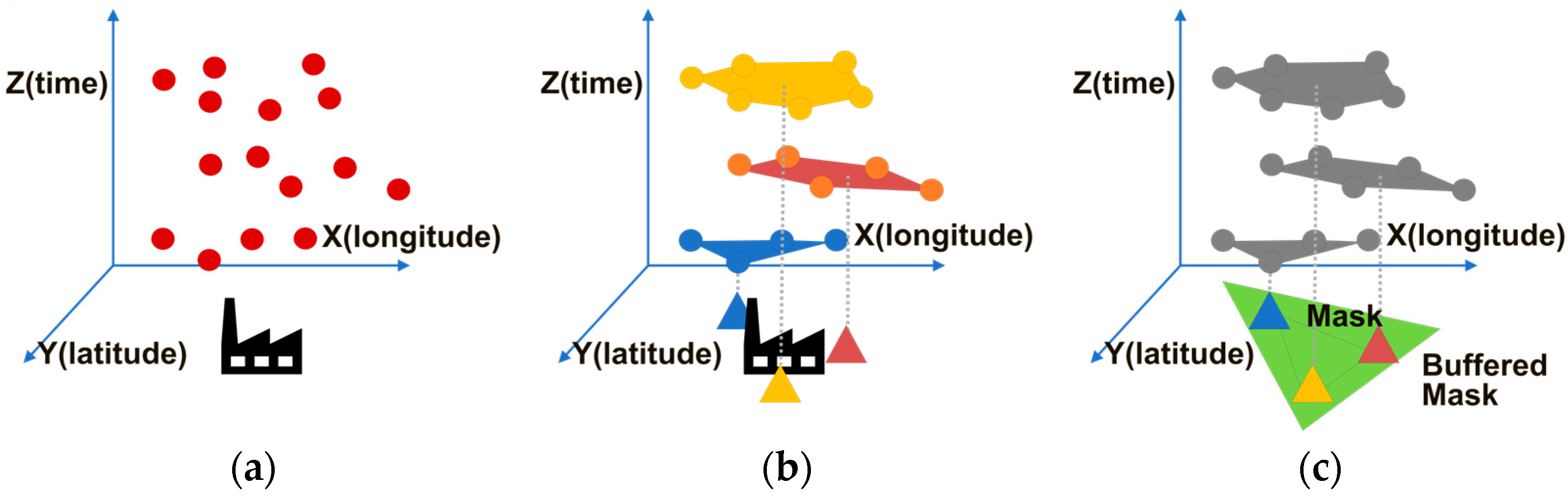
2.4.1. Stage 1—ST-MASK Processing

This study incorporates the detection of outliers and normal values, specifically recognizing normal industrial activities and allowing the identification of outliers as forest fires. It also includes masking with ST-DBSCAN (ST-MASK), which encompasses industrial activity areas and the VIIRS margin of error. Figure 6 describes the algorithm-building method for ST-MASK processing.

The initial step involves applying DBSCAN to hotspots collected over an extended period, combining the centroids of the formed clusters $D_C$ with the noise $D_N$ to create a simplified dataset. Figure 6a illustrates the outcome of this process.

The first step of Stage 1 can be expressed in Equation (1):

$$\begin{array}{c}DBSCAN\left(DB\right)\hspace{1em}\to \hspace{1em}clusters\hspace{1em}=\hspace{1em}\left\{C_1,\hspace{1em}{C}_2,\hspace{1em}\cdots \hspace{1em}{C}_n\right\},\hspace{1em}\hspace{1em}noise=\hspace{1em}\left\{N_1,\hspace{1em}{N}_2,\hspace{1em}\cdots \hspace{1em}{N}_m\right\},\\ \hspace{1em}{D}_C=\{\mathit{centroid}\left(C_i\right)\mid C_i\in \mathit{clusters}\},{ D}_N=\mathit{noise},\\ {DB}_U\hspace{1em}=\hspace{1em}{D}_C\hspace{1em}\cup \hspace{1em}{D}_N\end{array}$$

(1)

ST-DBSCAN clusters are subsequently generated for ${DB}_U$, and the centroids are extracted to reduce the three-dimensional (3D) data to 2D data ${STD}_C$, as described in Figure 6b. The second step of Stage 1 can be expressed in Equation (2):

$$\begin{array}{c}\mathit{ST}\_\mathit{DBSCAN}\left({DB}_U\right)\to \mathit{clusters}=\{S{C}_1,S{C}_2,\dots ,S{C}_n\}, \mathit{noise}=\{S{N}_1,S{N}_2,\dots ,S{N}_m\}\\ {STD}_C=\{\mathit{centroid}\left(S{C}_j\right)\mid S{C}_j\in \mathit{clusters}\}\end{array}$$

(2)

After eliminating the noise generated during the process, the centroid clusters are identified as normal activities that primarily create hotspots. Consequently, each cluster represents the scope of normal values.

As shown in Figure 6c, a convex hull process is applied to the generated clusters to extend the scope of VIIRS resolution, thereby calculating the final forest fire masking areas. For new data inputs, recalculation is performed to reflect the updated DBSCAN and centroids, ensuring that the algorithm adapts to the most recent information. The final step of Stage 1 can be expressed in Equation (3):

$$\begin{array}{c}\mathit{DBSCAN}\left({STD}_C\right)\to D_{{STD}_C}=\{M{C}_1,M{C}_2,\dots ,M{C}_q\}\\ \mathit{ST}\text{-}\mathit{MASK}=\{\mathit{buffer}\left(\mathit{convex}\_\mathit{hull}\left(M{C}_l\right)\right)\mid M{C}_l\in D_{{STD}_C}\}\end{array}$$

(3)

This methodology enables the identification and differentiation of hotspots caused by industrial activities from those resulting from forest fires.

In the study, the $minpts$ parameter for DBSCAN and ST-DBSCAN is set to 3, which represents the minimum number of polygons required to form a cluster. The $Eps1$ value is 2700 (m, UTM-K[EPSG5179]) and indicates the maximum distance a forest fire can spread by wind, as determined in [36]. Meanwhile, the $Eps2$ parameter in ST-DBSCAN was set at 10, considering the prolonged duration of forest fires. This value is based on the duration of the longest forest fire in South Korea (the Uljin-Samcheok forest fire), lasting 213 h. Additional hours are added to the $Eps2$ value to account for the potential impact of climate change on the duration of forest fires. The value to perform the buffer is set considering the resolution of the VIIRS and is set to 375 m, which is the resolution of the VIIRS used in this study.

2.4.2. Stage 2—Forest Fire Detection with Density-Based Spatial Clustering of Applications with Noise (DBSCAN)

This research study uses the distributor for identifying forest fire areas, which are calculated based on the cluster’s size estimated by calculating polygons from the borders of the cluster’s points. The convex hull algorithm is used for this purpose, as it represents the smallest set (area) of points that can be connected without extending beyond its border. This algorithm can be visualized as a stretched rubber band surrounding the set of points, the cluster.

The $minpts$ and $Eps$ parameters for DBSCAN are the same as the values used in Stage 1. In addition, ST-MASK polygon and LULC values are used to calculate forest fire areas. All point-type VIIRS data are filtered to exclude areas not included in ST-MASK. Then, the overlapping data in the LULC forest areas are filtered to remove hotspots in forests, forming a dataset exclusively consisting of hotspots caused by forest fires.

The resulting data are used to form polygons with DBSCAN, following the ST-MASK process described above. To exclusively identify the forest areas affected by fires from these polygon components, a secondary filtration is applied using LULC to identify the final forest fire areas.

2.5. Model Evaluation Methods

2.5.1. Generating Forest Fire Area with dNBR

The model is used to identify areas affected by forest fires. A dNBR ($\Delta NBR$) analysis is also conducted to verify the relative accuracy of the findings using the United States Geological Survey (USGS) burn severity index and satellite images.

$$NBR={\displaystyle \frac{\mathit{NIR}-\mathit{SWIR}}{\mathit{NIR}+SWIR}}$$

(4)

While Equation (4) is similar to NDVI, it is calculated using SWIR (Band 7, 2100–2280 nm) and NIR (Band 5, 850–880 nm) reflectance instead of visible light. NBR is calculated for both pre-fire and post-fire raster images.

$$\Delta NBR={NBR}_{pre\text{-}fire}-{NBR}_{post\text{-}fire}$$

(5)

Equation (5) shows that dNBR is calculated as the difference between ${NBR}_{pre\text{-}fire}$ and ${NBR}_{post\text{-}fire}$. It provides quantitative measurements of changes in vegetation caused by fire. Negative dNBR values indicate the regrowth of vegetation cover or the absence of burnt areas, whereas positive values can signify a set of burn severity values. A widely used classification system is the USGS burn severity universal thresholds, ranging from −0.5 to +1.3. In line with the Fire Effects Monitoring and Inventory System (FIREMON), the system is used to analyze the dNBR values accurately. FIREMON explains a classification with seven classes based on different dNBR ranges [19] (

Table 2. United States Geological Survey (USGS) difference-Normalized Burn Ratio (dNBR) classification [39].

Severity Level	dNBR Range (Scaled by 103)	dNBR Range (Not Scaled)
Enhanced Regrowth, high	−500 to −251	−0.500 to −0.251
Enhanced Regrowth, low	−250 to −101	−0.250 to −0.101
Unburned	−100 to +99	−0.100 to +0.99
Low Severity	+100 to +269	+0.100 to +0.269
Moderate–Low Severity	+270 to +439	+0.270 to +0.439
Moderate–High Severity	+440 to +659	+0.440 to +0.659
High Severity	+660 to +1300	+0.660 to +1.300

).

2.5.2. Comparing Polygon Region Similarity Based on DIoU

To verify the similarity of dNBR with the forest fire areas constructed in this study, we use DIoU. IoU, an evaluation technique that is the prototype of DIoU, is used in the field of object detection to measure similarity as a value between 0 and 1 using the intersection area and union area of two polygons and is calculated using the method in Equation (6) [40,41]. In Equation (6), $B$ is the prediction bounding box, and $B^{gt}$ is the ground truth. $B,B^{gt}\subseteq \mathbb{S}\in {\mathbb{R}}^n$ IoU can be computed when the conditions of [42,43] are as follows:

$$IoU(B,B^{gt})={\displaystyle \frac{Area of Overlap}{Area of Union}}={\displaystyle \frac{\mid B\cap B^{gt}\mid }{\mid B\cup B^{gt}\mid }}$$

(6)

The following advanced IoU algorithms have been proposed: GIoU, which is a method that uses Global Box, which means the smallest size that includes both polygons so that it can be evaluated even when two polygons do not overlap; DIoU, which uses the distance between centroids to impose a distance penalty; and CIoU, which calculates the aspect ratio or rotation in addition to DIoU. However, this study does not consider the aspect ratio or rotation relationship, so DIoU is used to measure similarity. The benefits of using DIoU are shown in Figure 7. In IoU or GIoU, if the overlapped area of two polygons is the same or if the area of overlap is 0, the same similarity is measured because the position of the polygons is not considered [44], but in the case of DIoU, if $B$ is $B^{gt}$, it can be calculated based on how close it is to the area of overlap, making it possible to effectively compare the area of the forest fire with the dNBR [45].

Equation (7) is the expression to calculate GIoU. $C$ denotes a convex object that contains both the bounding box and the ground truth; $B,B^{gt} \subseteq \mathbb{S}\in {\mathbb{R}}^n$; $C \subseteq \mathbb{S}\in {\mathbb{R}}^n.$ DIoU can be computed as follows:

$$GIoU=1-IoU-{\displaystyle \frac{\mid C\backslash (B\cup B^{gt})\mid }{\mid C\mid }}$$

(7)

Equation (8) is the expression for calculating DIoU. ${\rho }^2\left(B,B^{gt}\right)$ is the distance of the centroid between the predicted bounding box and the ground truth; $c$ is the diagonal length of rectangle $C$ containing both the bounding box and the ground truth.

$$DIoU=1-IoU+{\displaystyle \frac{{\rho }^2\left(B,B^{gt}\right)}{c^2}}$$

(8)

2.5.3. Comparison of Polygon Convex Similarity Based on Hausdorff Distance

The resulting forest fire areas in this study are represented by convex hull polygons of VIIRS point clusters. These are a characteristic that is not well quantified by IoUs alone, which is adequate to capture the degree of internal overlap. Therefore, we additionally use Hausdorff distance as a measure of similarity to the convex. Hausdorff distance is a metric that measures the maximum distance among a set of minimum distances between two polygons, sets of points, or lines [46,47,48], as shown in Figure 8. The Hausdorff distance of the convex hull of the forest fire area from the dNBR is used to verify similarity.

Equation (9) shows the computation of the Hausdorff distance $d_H\left(A,B\right)$ between two sets of points $A,B$. Given a set of two points $A,B,$ if point $a,\mathrm{b}$ is defined to be $a,b\in \mathbb{R}$ is, $d(a, b)$ denotes the distance between $a$ and $b.$ The distance is usually Euclidean distance. $sup$ is set $S$ for every element of $x$ that satisfies the distance between two points $f\left(x\right) \le f\left(s\right)$ for all elements in $s \in S$ among $f\left(s\right)$. The Hausdorff distance is the maximum value of $A$ for all points in $a$ for all points in $B$ for every point in $b$. After finding the smallest value among them, the distance to $B$ must be calculated for every point in $b$ and the distance to $A$ for every point in $a$. The largest of those will be used as the maximum value [49,50].

$$d_H\left(A,B\right):=max\left\{\underset{a\in A}{\mathit{sup}}d(a,B),\underset{b\in B}{\mathit{sup}}d(A,b)\right\}$$

(9)

3. Results

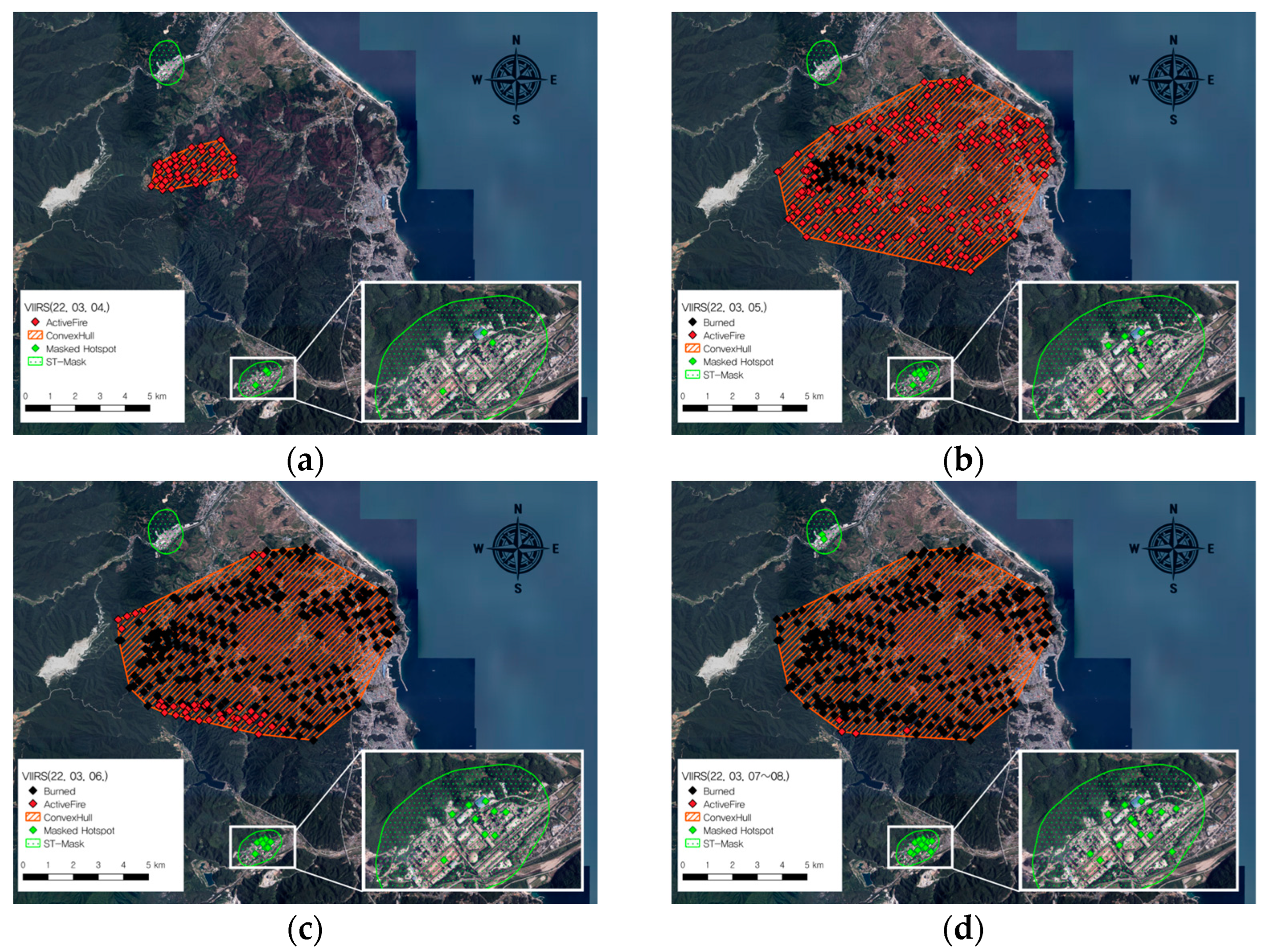
3.1. ST-MASK Generation and Classification Results

The analysis of datasets across South Korea yielded 428 ST-MASKs, providing a substantial sample size for this study. Subsequently, a more detailed examination of the components of the 21 ST-MASKs in Gangwon-do was conducted using the LULC dataset provided by the Ministry of Environment.

According to

Table 3. Components of buffers.

Land Use/ Land Cover 1 (LULC1) (Name)	Land Use/ Land Cover 1 (LULC1) (%)	Land Use/ Land Cover 2 (LULC2) (Name)	Land Use/ Land Cover 2 (LULC2) (%)
Used Area	34.87	Residential areas	9.98
		Commercial areas	6.94
		Public facility areas	6.02
		Industrial areas	5.60
		Traffic areas	3.79
		Cultural/sports/leisure facilities	2.54
Agricultural Lands	26.44	Crop fields	10.80
		Rice paddies	1.41
		Cultivation facilities	1.13
		Other agricultural lands	0.57
		Orchards	0.44
Forest	14.35	Broadleaf forests	4.28
		Coniferous forests	3.46
		Mixed forests	2.79
Grass	10.53	Artificial grass	26.33
		Natural grass	0.11
Wetlands	9.95	Inland wetlands	2.39
Barren	2.39	Other barren lands	9.37
		Natural barren lands	0.58
Waters	1.48	Inland waters	1.45
		Sea	0.03

, 35% of ST-MASKs were formed in urban and industrial areas, 10% in residential areas, and 26% in cultivation areas, 11% in crop fields. This finding suggests that the recurrent incineration of agricultural wastes or fires from such activities contributes significantly to the formation of ST-MASKs. The remaining 25% of ST-MASKs were formed in forest and grass areas.

When analyzing the centroids of ST-MASKs, 11 were detected as factories, 4 as solar panel reflections, and 6 as other facilities (leisure, construction, and military). The distribution of FRP, fire pixel brightness temperature, and fire pixel brightness temperature (T31) in the buffer (Figure 9a–c) were examined for factories and solar panels, excluding other facilities.

The kernel density estimation (KDE) results show that factories and solar panels exhibit significantly different values. However, the values of the hotspot observation data caused by solar panel reflection are very small compared to the forest fire points, making it difficult to classify them numerically because the spectrum of forest fires includes all false positive spectral bands.

The analysis of 22,209 hotspot events detected in Gangwon-do from February 2012 to August 2022 revealed four cases. The possibility to remove 17,682 Case A hotspots (79.6%) with LULC-only filtering was established, whereas ST-MASK filtering can remove 20,899 Case D hotspots (94.1%).

A total of 3627 non-forest-fire events (16.33%) were found in ST-MASK areas, which means ST-MASKs can eliminate Case D hotspots that LULC cannot remove. In addition, 91 Case B hotspots (0.41%) were removed in the DBSCAN process. A comparison of the results with the South Korea Forest Service (KFS) literature was conducted, which confirmed that 13 of the 18 cases of at least 30 ha forest fires had been detected without noise. The other five fires seem to have been filtered out as Case B events because the raw VIIRS data did not reach the effective DBSCAN min-sample value due to adverse weather conditions.

3.2. Model Validation Results

To review the results of ST-MASK application, images from 5 March 2022 to 9 March 2022 were tested. This period was chosen because multiple large forest fires occurred simultaneously in Gangwon-do during this time. In the Gangneung/Donghae area within the province, there are several large cement production plants located near forests. Figure 10 presents the results of ST-MASK and DBSCAN-based area calculation using dNBR and VIIRS for the four forest fires that occurred over four days, including the fire shown in Figure 10. The final true values are based on the field survey results of the forest fire lists provided by the KFS. A comparison of the dNBR results with the study findings confirmed that the VIIRS results tend to overestimate the observed values compared to dNBR for small fires. However, for large fires, the DBSCAN results demonstrate higher accuracy (

Table 4. Forest fire detection results by area.

Case	Korea Forest Service (KFS) Results (ha)	Visible Infrared Imaging Radiometer Suite (VIIRS) (ha)		Difference-Normalized Burn Ratio (dNBR) (ha)
		Pred.	Diff.	Pred.	Diff.
Seongsan-myeon, Gangneung-si, Gangwon-do	30.89	15.47	−50.64%	16.2	−47.71%
Buk-myeon, Uljin-gun, Gyeongsangbuk-do	4190.4	5284.72	+26.12%	8545.9	+103.94%
Okgye-myeon, Gangneung-si, Gangwon-do	18463	20465.05	+10.84%	56026	+203.45%
Gimsatgat-meon, Yeongwol-gun, Gangwon-do	184.01	664.34	+61.03%	191.74	+4.20%

).

For further interpretation of the results, DIoU and Hausdorff distance were calculated based on the results of analyzing the shape with dNBR to check the difference in shape (Figure 11). As the calculation of this result should be performed with a single polygon, LULC was not intersected in the prediction result of VIIRS, and in the case of dNBR, pixels with low severity or higher were used, and to prevent the enlarged interpretation due to noise of a single pixel, a convex hull was performed after morphology calculation with an opening operation on binary pixels using a 3 × 3 pixel mask. The results of the comparison of the two polygons show that, similar to the comparison of the area, the difference in shape is large for small fires, but there is little difference for large fires. In the case of DIoU, the overall score is low because it does not reflect the evaluation of the area, but the Hausdorff distance is short, so it is necessary to look at both indicators to interpret the results comprehensively.

The case of the Okgye-myeon forest fire (Figure 11c), which occurred on 4 March 2022 near a plant (Figure 12), illustrates a single ST-MASK, with each of the 10-year points that constitute it being assigned a color representing a specific time range corresponding to $Eps2$ from ST-DBSCAN. The yellow area represents the forest fire area detected by dNBR, while the green areas depict ST-MASK, with green points indicating hotspots caused by industrial activities detected on 4 March 2022. The red areas show the portions of the finalized forest fires, with red points indicating hotspots recognized as actual forest fires.

These hotspots, if monitored solely using VIIRS source data, could be erroneously identified as forest fires, potentially leading to an overestimation of fire extent. However, the ST-MASK algorithm effectively eliminates these false positives in the initial stages of processing, enabling a more accurate assessment of forest fire dimensions.

Figure 13 illustrates the disparity in Hausdorff distance and DIoU when ST-MASK is not applied. Without ST-MASK, the Hausdorff distance is calculated to be 1944 m larger, and the DIoU is 10 points lower compared to results with ST-MASK applied. This discrepancy arises from a miscalculation in the final clustering result due to the influence of the power plant in the upper right region. In this scenario, ST-MASK effectively addresses case D, demonstrating not only enhanced recognition accuracy but also an improved detection of false positives.

Figure 14 illustrates the clustering process of accumulated hotspots from 4 to 9 March 2022 without ST-MASK application. Red dots represent hotspots occurring on the specified dates, while the orange dashed area delineates the recognized forest fire extent.

In this plot, cumulative results are utilized, with hotspots occurring before the target date marked as black dots. False positive hotspots were detected on all dates except in Figure 14c, where three or more points can form clusters and convex hull results, leading to false positive fire reports. Figure 14d further demonstrates how power plant influence distorts forest fire area formation.

Figure 15 depicts the accumulated hotspot clustering process with ST-MASK applied. Green dots represent all accumulated false positive hotspots, while the green dotted area denotes the ST-MASK region. This visualization demonstrates that all false positive hotspots are filtered within the ST-MASK area, resulting in the recognition of legitimate forest fire areas without distortion or false positives.

4. Discussion

Previous studies either used DBSCAN to determine the size of a particular forest fire or ST-DBSCAN to determine the progress of a forest fire. However, this study tried a new approach that combines both methodologies by taking advantage of the fact that forest fire patterns show an unusual pattern compared to those of industrial facilities. The potential to utilize its results through a comparison with the findings of dNBR, a widely used forest fire extent estimation method, was also assessed.

The discussion and implications of this research are as follows:

(1)

ST-MASK was used to distinguish between forest fires and industrial facilities, and the latter were classified as solar power plants and factories. When attributes of VIIRS were compared, factories and solar panels showed significant differences on the infrared spectrum. However, the value of the hotspot observation data due to solar panel reflections was very small compared to forest fire spots. Moreover, the forest fire spectrum contained false positive spectral bands. As a result, it was concluded that it is difficult to classify them numerically.

(2)

As of 2024, the highest resolution of VIIRS to detect hotspots is 375 m (SUOMI NPP). If the resolution of the hotspot is lower than land cover, false positive hotspots can remain even when masked by land cover. On the other hand, ST-MASK filtering can remove 94% of false positive hotspots, which represents a 16.33% noise reduction compared to LULC masking (based on August 2022 Gangwon-do data).

(3)

To justify the use of ST-MASK, a comparison of VIIRS based on the KFS survey and remote sensing results using dNBR was performed. The dNBR provides relatively accurate results for small forest fires, while VIIRS data improve accuracy for large forest fires of >1000 ha. However, depending on the shape of the forest fire, forest fire areas larger than 15 ha may be lost in processing due to resolution issues. Moreover, it is confirmed that there are missing VIIRS data in the case of forest fires extinguished within a short period (e.g., the Gangneung forest fire, 11 April 2023), which shows that the method developed in this study can remove false positives in prolonged large fires with greater effectiveness than conventional methods. After comparing the convergence of VIIRS and dNBR using IoU and the Hausdorff distance, this study found that, as with the area comparison, there is a large difference in the shape of the polygons for small fires due to differences in the resolution of the mutual data, but little difference for large fires. For DIoU, the accuracy of small fires was underestimated due to the lack of area assessment, but due to the short Hausdorff distance, it is necessary to look at both metrics and interpret the results collectively.

(4)

After investigating the shape generation of forest fires with ST-MASK and without it for the forest fire in Gangneung-si, Gangwon-do, it was confirmed that ST-MASK normally performs the scenario described in Case D, mentioned in Figure 2. However, there were two errors. First, when ST-MASK was not applied, factory activity was recognized as a forest fires (false recognition of forest fire). And the size of the forest fire was incorrectly calculated (polygon distortion error).

(5)

The findings in (1)–(4) suggest that ST-MASK is useful for determining forest fires in VIIRS hotspots and eliminating hotspots that cannot be removed with LULC data. However, this study has a potential limitation in that recently installed heat-emitting facilities can be recognized as fires due to absence of an ST-MASK because there are not enough false positive hotspot data to form the mask. This limitation is due to the shortcoming of the technique to detect false positives using long-term hotspots, which cannot collect enough clusters from the false positive hotspot data for recently installed facilities. Therefore, to overcome this limitation, this study proposes a complementary method, forming an ST-MASK with fewer than three hotspots, i.e., the minimum number of hotspots that form a convex hull polygon. To validate false positive areas with fewer hotspots, this study simultaneously uses hyperspectral vegetation indices NDVI and NBR. Generally, high-resolution satellites such as Sentinel or Landsat are used to calculate these indices as in this study, but VIIRS can also obtain coarse-resolution NDVI and NBR. It includes the Red (I1; 0.64 nm), SWIR (I2; 0.865 nm), and NIR (I3; 1.61 nm) bands, which can be used to justify false positive hotspots.

5. Conclusions

In the past, efforts to build forest fire databases have relied on collaboration between governments and transnational organizations. When identifying specific forest fires proves challenging, satellite remote sensing is used to determine the occurrence and extent of forest fires. Due to the geographical characteristics of Korean Peninsula, where most of the country is surrounded by forests, forest fires, both large and small, occur frequently in relation to the size of the country. In particular, Gangwon province is composed of forests, and many industrial and residential facilities are located within these forests. For this reason, Gangwon province is highly vulnerable to forest fires. Remote sensing methods are often used to track and monitor forest fires, but these methods have some limitations. For example, NBR-based techniques can take a long time for satellites to scan the desired area and are highly affected by cloud cover. These limitations make it difficult to detect and respond to forest fires quickly and accurately. Active fire detection techniques also present issues, especially in South Korea, where many industrial facilities emit heat, resulting in Fire Radiative Power (FPR). This causes noise in the forest fire detection process, making it difficult to accurately identify actual forest fires. However, for regions that do not track forest fire statistics, where data are often unavailable or missing, should solve these problems that require a complex process.

In this study, we propose an ST-MASK technique using patterns of forest fires and industrial facilities to solve these problems. This study’s significance lies in the development of ST-MASK, a method that filters hotspots without necessitating the separation of non-forested areas or extraction of forested areas through computationally intensive land cover analysis. The DBSCAN algorithm, a machine learning model for outlier detection and clustering, is employed to differentiate between routine heat generation in industrial facilities and unusual fire events. This study applies VIIRS data with a 375 m resolution. Future research could optimize this process by incorporating diverse remote-sensing data inputs. While DBSCAN was utilized for clustering in this study, various DBSCAN algorithms exist, including ST-DBSCAN.

The application of multiple algorithms could enhance research depth and segment roles, leading to techniques applicable across diverse fields. These advantages are expected to address various analytical challenges. Contemporary data analysis extends beyond remote sensing to a wide array of collected data. While some data can be easily distinguished through inherent attributes, spatial data often lack structured attributes. For three-dimensional datasets comprising location and time elements, ST-MASK can efficiently create representative regions, detect noise, and filter or extract information. This approach is applicable even to non-spatial data. A typical application of outlier detection algorithms is machine fault or failure detection. ST-MASK can generate masks of normal machine operating ranges using x and y coordinates and create polygons representing outlier patterns for failure analysis. This innovative approach offers the potential for enhancing data analysis and outlier detection across various domains, from remote sensing to industrial applications, by providing a more efficient and adaptable method for pattern recognition and anomaly detection.

References

1. Chae, H.; Ahn, J.; Choi, J. Forest Fire Area Extraction Method Using VIIRS. Korean J. Remote Sens. 2022, 38, 669–683. [Google Scholar] [CrossRef]
2. Briones-Herrera, C.I.; Vega-Nieva, D.J.; Monjarás-Vega, N.A.; Briseño-Reyes, J.; López-Serrano, P.M.; Corral-Rivas, J.J.; Alvarado-Celestino, E.; Arellano-Pérez, S.; Álvarez-González, J.G.; Ruiz-González, A.D.; et al. Near real-time automated early mapping of the perimeter of large forest fires from the aggregation of VIIRS and MODIS active fires in Mexico. Remote Sens. 2020, 12, 2061. [Google Scholar] [CrossRef]
3. Giglio, L.; Randerson, J.T.; van der Werf, G.R.; Kasibhatla, P.S.; Collatz, G.J.; Morton, D.C.; DeFries, R.S. Assessing variability and long-term trends in burned area by merging multiple satellite fire products. Biogeosciences 2010, 7, 1171–1186. [Google Scholar] [CrossRef]
4. Land Atmosphere Near Real-Time Capability for EOS Fire Information for Resource Management System. VIIRS (S-NPP) I Band 375 m Active Fire locations NRT (Vector Data) [Dataset]. 2021. Available online: https://www.earthdata.nasa.gov/learn/find-data/near-real-time/firms/vnp14imgtdlnrt (accessed on 18 July 2024).
5. Artés, T.; Oom, D.; de Rigo, D.; Durrant, T.H.; Maianti, P.; Libertà, G.; San-Miguel-Ayanz, J. A global wildfire dataset for the analysis of fire regimes and fire behaviour. Sci. Data 2019, 6, 296. [Google Scholar] [CrossRef] [PubMed]
6. Cardil, A.; Monedero, S.; Ramírez, J.; Silva, C.A. Assessing and reinitializing wildland fire simulations through satellite active fire data. J. Environ. Manag. 2019, 231, 996–1003. [Google Scholar] [CrossRef]
7. Ester, M.; Kriegel, H.P.; Sander, J.; Xu, X. A density-based algorithm for discovering clusters in large spatial databases with noise. In Proceedings of the Second International Conference on Knowledge Discovery and Data Mining, Portland, OR, USA, 2–4 August 1996; Volume 96, pp. 226–231. [Google Scholar] [CrossRef]
8. Birant, D.; Kut, A. ST-DBSCAN: An algorithm for clustering spatial–temporal data. Data Knowl. Eng. 2007, 60, 208–221. [Google Scholar] [CrossRef]
9. Youn, H.; Jeong, J. Detection of forest fire and NBR mis-classified pixel using multi-temporal Sentinel-2a images. Korean J. Remote Sens. 2019, 35, 1107–1115. [Google Scholar] [CrossRef]
10. Zhang, X.; Waugh, D.W.; Orbe, C. Dependence of northern hemisphere tropospheric transport on the midlatitude jet under abrupt CO2 increase. J. Geophys. Res. Atmos. 2023, 128, e2022JD038454. [Google Scholar] [CrossRef]
11. Rouse, J.W.; Haas, R.H.; Schell, J.A.; Deering, D.W. Monitoring vegetation systems in the great plains with ERTS. NASA Spec. Publ. 1974, 351, 309. Available online: https://ntrs.nasa.gov/api/citations/19740022614/downloads/19740022614.pdf (accessed on 18 July 2024).
12. López-García, M.J.; Caselles, V. Mapping burns and natural reforestation using thematic Mapper data. Geocarto Int. 1991, 6, 31–37. [Google Scholar] [CrossRef]
13. Roy, S.; Lane, T.; Allen, C.; Aragon, A.D.; Werner-Washburne, M. A hidden-state markov model for cell population deconvolution. J. Comput. Biol. 2006, 13, 1749–1774. [Google Scholar] [CrossRef] [PubMed]
14. Key, C.H.; Benson, N. Measuring and remote sensing of burn severity: The CBI and NBR. In Proceedings of the Joint Fire Science Conference and Workshop, Boise, ID, USA, 15–17 June 1999; Volume 2, p. 284. Available online: https://www.frames.gov/documents/catalog/key_benson_1999_MeasuringRemoteSensingBurnSeverityCBIandNBR_poster.pdf (accessed on 18 July 2024).
15. Pepe, M.; Parente, C. Burned area recognition by change detection analysis using images derived from Sentinel-2 satellite: The case study of Sor-rento Peninsula, Italy. J. Appl. Eng. Sci. 2018, 16, 225–232. [Google Scholar] [CrossRef]
16. Jin, Y.; Randerson, J.T.; Goetz, S.J.; Beck, P.S.A.; Loranty, M.M.; Goulden, M.L. The influence of burn severity on postfire vegetation recovery and albedo change during early succession in North American boreal forests. J. Geophys. Res. Biogeosci. 2012, 117. [Google Scholar] [CrossRef]
17. Karau, E.C.; Keane, R.E. Burn severity mapping using simulation modelling and satellite imagery. Int. J. Wildland Fire 2010, 19, 710–724. [Google Scholar] [CrossRef]
18. Navarro, G.; Caballero, I.; Silva, G.; Parra, P.-C.; Vázquez, Á.; Caldeira, R. Evaluation of forest fire on Madeira Island using Sentinel-2A MSI imagery. Int. J. Appl. Earth Obs. Geoinf. 2017, 58, 97–106. [Google Scholar] [CrossRef]
19. Lutz, J.A.; Key, C.H.; Kolden, C.A.; Kane, J.T.; van Wagtendonk, J.W. Fire frequency, area burned, and severity: A quantitative approach to defining a normal fire year. Fire Ecol. 2011, 7, 51–65. [Google Scholar] [CrossRef]
20. Schepers, L.; Haest, B.; Veraverbeke, S.; Spanhove, T.; Vanden Borre, J.; Goossens, R. Burned area detection and burn severity assessment of a heathland fire in Belgium using airborne imaging spectroscopy (APEX). Remote Sens. 2014, 6, 1803–1826. [Google Scholar] [CrossRef]
21. Lee, S.; Kim, G.; Kim, Y.; Kim, J.; Lee, Y. Development of FBI(Fire Burn Index) for Sentinel-2 images and an experiment for detection of burned areas in Korea. J. Assoc. Korean Photo-Geogr. 2017, 27, 187–202. [Google Scholar] [CrossRef]
22. Matson, M.; Dozier, J. Identification of subresolution high temperature sources using a thermal IR sensor. Photo-Grammetric Eng. Remote Sens. 1981, 47, 1311–1318. Available online: https://www.asprs.org/wp-content/uploads/pers/1981journal/sep/1981_sep_1311-1318.pdf (accessed on 18 July 2024).
23. Matson, M.; Holben, B. Satellite detection of tropical burning in Brazil. Int. J. Remote Sens. 1987, 8, 509–516. [Google Scholar] [CrossRef]
24. Zhang, T.; Wooster, M.J.; Xu, W. Approaches for synergistically exploiting VIIRS I- and M-Band data in regional active fire detection and FRP assessment: A demonstration with respect to agricultural residue burning in Eastern China. Remote Sens. Environ. 2017, 198, 407–424. [Google Scholar] [CrossRef]
25. Dong, B.; Li, H.; Xu, J.; Han, C.; Zhao, S. Spatiotemporal Analysis of Forest Fires in China from 2012 to 2021 Based on Visible Infrared Imaging Radiometer Suite (VIIRS) Active Fires. Sustainability 2023, 15, 9532. [Google Scholar] [CrossRef]
26. Barber, C.B.; Dobkin, D.P.; Huhdanpaa, H. The quickhull algorithm for convex hulls. ACM Trans. Math. Softw. 1996, 22, 469–483. [Google Scholar] [CrossRef]
27. Fisher, D.; Wooster, M.J. Shortwave IR adaption of the mid-infrared radiance method of fire radiative power (FRP) retrieval for assessing industrial gas flaring output. Remote Sens. 2018, 10, 305. [Google Scholar] [CrossRef]
28. Campus, A.; Laiolo, M.; Massimetti, F.; Coppola, D. The transition from MODIS to VIIRS for global volcano thermal monitoring. Sensors 2022, 22, 1713. [Google Scholar] [CrossRef] [PubMed]
29. Coskuner, K. Assessing the performance of MODIS and VIIRS active fire products in the monitoring of wildfires: A case study in Turkey. Iforest—Biogeosci. For. 2022, 15, 85–94. [Google Scholar] [CrossRef]
30. Sofan, P.; Yulianto, F.; Sakti, A.D. Characteristics of false-positive active fires for biomass burning monitoring in Indonesia from VIIRS data and local geo-features. ISPRS Int. J. Geo-Inf. 2022, 11, 601. [Google Scholar] [CrossRef]
31. National Institute of Biological Resources. Biodiversity of the Korean Peninsula. Available online: https://species.nibr.go.kr/ (accessed on 2 July 2024).
32. Ying, H.; Shan, Y.; Zhang, H.; Yuan, T.; Rihan, W.; Deng, G. The Effect of Snow Depth on Spring Wildfires on the Hulunbuir from 2001–2018 Based on MODIS. Remote Sens. 2019, 11, 321. [Google Scholar] [CrossRef]
33. Ministry of Environment (South Korea) LandCoverMap. Available online: https://egis.me.go.kr/intro/land.do (accessed on 2 July 2024).
34. USGS EarthExplorer. Available online: https://earthexplorer.usgs.gov/ (accessed on 2 July 2024).
35. Xu, D.; Tian, Y. A Comprehensive Survey of Clustering Algorithms. Ann. Data Sci. 2015, 2, 165–193. [Google Scholar] [CrossRef]
36. Storey, M.A.; Price, O.F.; Bradstock, R.A.; Sharples, J.J. Analysis of Variation in Distance, Number, and Distribution of Spotting in Southeast Australian Wildfires. Fire 2020, 3, 10. [Google Scholar] [CrossRef]
37. Alahmari, A.; Jamal, A.; Elazhary, H. Comparative Study of Common Density-Based Clustering Algorithms. In Proceedings of the 2021 National Computing Colleges Conference (NCCC), Taif, Saudi Arabia, 27–28 March 2021; pp. 1–6. [Google Scholar]
38. Schubert, E.; Sander, J.; Ester, M.; Kriegel, H.P.; Xu, X. DBSCAN revisited, revisited: Why and how you should (still) use DBSCAN. ACM Trans. Database Syst. 2017, 42, 1–21. [Google Scholar] [CrossRef]
39. Lutes, D.C.; Keane, R.E.; Caratti, J.F.; Key, C.H.; Benson, N.C.; Sutherland, S.; Gangi, L.J. FIREMON: Fire Effects Monitoring and Inventory System; U.S. Department of Agriculture, Forest Service, Rocky Mountain Research Station: Fort Collins, CO, USA, 2006. [CrossRef]
40. Padilla, R.; Netto, S.L.; da Silva, E.A.B. A Survey on Performance Metrics for Object-Detection Algorithms. In Proceedings of the 2020 International Conference on Systems, Signals and Image Processing (IWSSIP), Niteroi, Brazil, 1–3 July 2020; pp. 237–242. [Google Scholar]
41. Gower, J.C.; Legendre, P. Metric and Euclidean properties of dissimilarity coefficients. J. Classif. 1986, 3, 5–48. [Google Scholar] [CrossRef]
42. Badhan, M.; Shamsaei, K.; Ebrahimian, H.; Bebis, G.; Lareau, N.P.; Rowell, E. Deep Learning Approach to Improve Spatial Resolution of GOES-17 Wildfire Boundaries Using VIIRS Satellite Data. Remote Sens. 2024, 16, 715. [Google Scholar] [CrossRef]
43. Chen, Y.; Hantson, S.; Andela, N.; Coffield, S.R.; Graff, C.A.; Morton, D.C.; Ott, L.E.; Foufoula-Georgiou, E.; Smyth, P.; Goulden, M.L.; et al. California wildfire spread derived using VIIRS satellite observations and an object-based tracking system. Sci. Data 2022, 9, 249. [Google Scholar] [CrossRef] [PubMed]
44. Rezatofighi, H.; Tsoi, N.; Gwak, J.; Sadeghian, A.; Reid, I.; Savarese, S. Generalized Intersection Over Union: A Metric and a Loss for Bounding Box Regression. In Proceedings of the IEEE Conference on Computer Vision and Pattern Recognition 2019, Long Beach, CA, USA, 15–20 June 2019; pp. 658–666. [Google Scholar] [CrossRef]
45. Zheng, Z.; Wang, P.; Liu, W.; Li, J.; Ye, R.; Ren, D. Distance-IoU Loss: Faster and Better Learning for Bounding Box Regression. In Proceedings of the AAAI Conference on Artificial Intelligence, New York, NY, USA, 7–12 February 2020; Volume 34, pp. 12993–13000. [Google Scholar] [CrossRef]
46. Kong, L.; Qian, H.; Xie, L.; Huang, Z.; Qiu, Y.; Bian, C. Multilevel Regularization Method for Building Outlines Extracted from High-Resolution Remote Sensing Images. Appl. Sci. 2023, 13, 12599. [Google Scholar] [CrossRef]
47. Masson, T.; Dumont, M.; Mura, M.D.; Sirguey, P.; Gascoin, S.; Dedieu, J.-P.; Chanussot, J. An Assessment of Existing Methodologies to Retrieve Snow Cover Fraction from MODIS Data. Remote Sens. 2018, 10, 619. [Google Scholar] [CrossRef]
48. Chen, Y.; He, F.; Wu, Y.; Hou, N. A local start search algorithm to compute exact Hausdorff Distance for arbitrary point sets. Pattern Recognit. 2017, 67, 139–148. [Google Scholar] [CrossRef]
49. Dey, E.K.; Awrangjeb, M. A Robust Performance Evaluation Metric for Extracted Building Boundaries from Remote Sensing Data. IEEE J. Sel. Top. Appl. Earth Obs. Remote Sens. 2020, 13, 4030–4043. [Google Scholar] [CrossRef]
50. Deza, E.; Deza, M.M. Encyclopedia of Distances; Springer Nature: Dordrecht, The Netherlands, 2009. [Google Scholar] [CrossRef]
Figure 1. Map of the study area. The area in purple is the provincial boundary map of South Korea. The orange area shows the area of Gangwon Province.
Remotesensing 16 02667 g001
Figure 2. Four cases of Visible Infrared Imaging Radiometer Suite (VIIRS) hotspot occurrence.
Remotesensing 16 02667 g002
Figure 3. Flow chart of this study.
Remotesensing 16 02667 g003
Figure 4. Diagram of the Density-Based Spatial Clustering of Applications with Noise (DBSCAN) algorithm. Circles in blue represent noise that does not belong in any cluster.
Remotesensing 16 02667 g004
Figure 5. Clustering results of Spatio-Temporal Density-Based Spatial Clustering of Applications with Noise (ST-DBSCAN) algorithm: (a) Gaussian data; (b) cluster results; Red dots mean noise, and the other colours mean points in clusters.
Remotesensing 16 02667 g005
Figure 6. ST-MASK Processing: (a) original data; The red dots mean raw hotspots. (b) reducing dimensions; Each colors represent the clusters created. (c) creating ST-MASK; Green polygon means ST-MASK.
Remotesensing 16 02667 g006
Figure 7. When comparing two rectangles, IoU and GIoU interpret incomplete differences if the ground truth contains a bounding box, but DIoU can compute the metric by calculating the distance of the values at the centroid.
Remotesensing 16 02667 g007
Figure 8. Process of calculating the Hausdorff distance. Two Hausdorff distances can be calculated when A, in green, is the predicted region and B, in orange, is the region generated from the hotspot.
Remotesensing 16 02667 g008
Figure 9. Kernel density estimation (KDE) plots of forest fire and in-buffer facility: (a) KDE plot of Fire Radiative Power (FRP); (b) KDE plot of brightness; (c) KDE plot of Bright_T31.
Remotesensing 16 02667 g009
Figure 10. Forest fire and incinerator distinction applied to hotspot data of March 2022 in South Korea: (a) 4 March 2022; Seongsan-myeon, Gangneung-si, Gangwon-do; (b) 4 March 2022; Buk-myeon, Uljin-gun, Gyeongsangbuk-do; (c) 4 March 2022; Okgye-myeon, Gangneung-si, Gangwon-do; (d) 4 March 2022; Gimsatgat-myeon, Yeongwol-gun, Gangwon-do.
Remotesensing 16 02667 g010
Figure 11. Plot of calculated Hausdorff distance (in 1) and DIoU (in 2): (a) 4 March 2022; Seongsan-myeon, Gangneung-si, Gangwon-do; (b) 4 March 2022; Buk-myeon, Uljin-gun, Gyeongsangbuk-do; (c) 4 March 2022; Okgye-myeon, Gangneung-si, Gangwon-do; (d) 4 March 2022; Gimsatgat-myeon, Yeongwol-gun, Gangwon-do. In n-1, The red cross represents furthest point.
Remotesensing 16 02667 g011
Figure 12. Forest fire and incinerator distinction applied to hotspot data of 4–8 March 2022. Gangneung-si, South Korea. The left figure illustrates that ST-MASK is generated by a high level of noise, with each color representing a discrete temporal interval.
Remotesensing 16 02667 g012
Figure 13. Hausdorff distance and DIoU calculation plot of the Okgye-myeon forest fire, which occurred on 4 March 2022, in Gangneung-si, Gangwon-do, South Korea, without the application of ST-MASK: (a) Hausdorff distance; The red cross represents furthest point. (b) DIoU.
Remotesensing 16 02667 g013
Figure 14. False alarms and forest fire progression without ST-MASK applied, 4–9 March 2022, Gangneung-si, Gangwon-do, South Korea: (a) 4 March 2022; (b) 5 March 2022; (c) 6 March 2022; (d) 7–9 March 2022.
Remotesensing 16 02667 g014
Figure 15. False alarms and forest fire progression with ST-MASK applied, 4–9 March 2022, Gangneung-si, Gangwon-do, South Korea: (a) 4 March 2022; (b) 5 March 2022; (c) 6 March 2022; (d) 7–9 March 2022.
Remotesensing 16 02667 g015