Estimation of Actual Evapotranspiration and Water Stress in Typical Irrigation Areas in Xinjiang, Northwest China

Abstract

The increasing water demand and the disparities in the spatiotemporal distribution of water resources will lead to increasingly severe water shortages in arid areas. Accurate evapotranspiration estimation is the basis for evaluating water stress and informing sustainable water resource management. In this study, we constructed a surface energy balance algorithm for land (SEBAL) model based on the Google Earth Engine platform to invert the actual evapotranspiration (ETa) in typical irrigation areas in Xinjiang, northwest China, during the growing season from 2005 to 2021. The inversion results were evaluated using the observed evaporation data and crop evapotranspiration estimated by the FAO Penman–Monteith method. The water stress index (WSI) was then calculated based on the simulated ETa. The impacts of climatic factors, hydrological conditions, land-use change, and irrigation patterns on ETa and WSI were analyzed. The results indicated the following: (1) The ETa simulated by the SEBAL model matched well with the observed data and the evapotranspiration estimated using the FAO Penman–Monteith approach, with correlation coefficients greater than 0.7. (2) The average ETa was 704 mm during the growing season, showing an increasing trend in the irrigation area of the Yanqi Basin (IAY), whereas for the irrigation area of Burqin (IAB) the average ETa was 677 mm during the growing season, showing an increasing trend. The land cover type mainly influenced the spatial distribution of ETa in the two study areas. (3) The WSI in both irrigation areas exhibited a decreasing trend, with the WSI in the IAY lower than that in the IAB. (4) Climate warming, increases in irrigation areas, and changes in cropping patterns led to increased ETa in the IAY and IAB; the overall decreasing trend in the WSI derived from the popularization of agricultural water-saving irrigation patterns in both regions, which reduces ineffective evapotranspiration and contributes positively to solving the water shortage problem in the basins. This study provides insight into water resource management in the Xinjiang irrigation areas.

1. Introduction

Water resources are essential to the sustainable development of depleted ecosystems, the environment, and the social economy. In March 2020, the United Nations released the World Water Development Report, stating that the global water demand is increasing by 1% per year [1]. Many regions have experienced varying levels of water stress [2,3]. Water stress is expected to increase worldwide, particularly in arid regions, due to population growth, socioeconomic development, and climate change [4,5]. Understanding the characteristics of water stress in different regions is critical to promoting the sustainable utilization of water resources.

Many previous studies have proposed various water stress indices to assess water resource stress at different spatiotemporal scales. However, existing water stress studies have mainly focused on national, provincial, and municipal administrative units, with less attention paid to water stress status at the basin or sub-basin scale, especially in oases. Water scarcity is particularly severe in the tail oases of the inland river basins in Xinjiang. On the one hand, the oases in Xinjiang are in an arid region that receives the least precipitation due to its geographical location, distance from the ocean, and terrain barriers. Moreover, the oases are the dominant dissipation areas of water resources in the basin. On the other hand, owing to agricultural development and rapid population expansion, the ecological environment continues to deteriorate, and the human–land relationship remains out of balance in oases.

The water stress index (WSI) is defined as the ratio of actual evapotranspiration (ETa) to potential evapotranspiration (PET) [6], which reflects the comprehensive impact of soil or vegetation water supply and demand, irrigation efficiency, and water use efficiency. The WSI has been used to assess water stress in arid regions. For example, Jiang et al. [7] employed the WSI to monitor the spatiotemporal features of water stress in the Aral Sea basin, and Jahangir et al. [8] used the index to study the changes in water stress for different land cover types in Iran. Evapotranspiration is a key factor in estimating regional water stress. However, the precise assessment of WSI is hindered because the accurate estimation of evapotranspiration at spatiotemporal scales remains challenging [9]. Given the spatial variations in climate conditions and surface heterogeneity, the spatiotemporal distribution of surface evapotranspiration varies greatly, making it difficult to accurately estimate evapotranspiration on a regional scale [10].

Traditional evapotranspiration evaluation methods are suitable for small areas [11]. The FAO Penman–Monteith method and crop coefficients can be integrated to estimate crop water demands; however, fine cropping structure information is difficult to obtain for most basins [12]. Enhanced remote sensing techniques have recently made it possible to estimate regional ETa using satellite images. Based on satellite images, existing ETa inversion methods can be categorized into two groups according to the model’s drivers: data-driven and process-driven physical inversion. Data-driven methods include empirical regression methods [4,13,14,15], machine learning methods [16,17,18,19], and data fusion methods [20,21,22]. The advantage of data-driven methods is that they can capture relationships within data. However, high-precision inversion results are highly dependent on high-quality driving data. In terms of most data-driven methods, the lack of explanations for the evapotranspiration process characterizes the methods as having limited interpretability in analyzing the estimation results. Process-driven physical inversion methods include the temperature–vegetation index eigenspace method [23,24], methods based on the Priestley–Taylor or Penman–Monteith formulae [25,26], and the energy balance residual algorithm [27,28,29]. These methods have good physical foundations. As a type of energy balance residual algorithm, the Surface Energy Balance Algorithm for Land (SEBAL) simplifies actual land surface processes, has a physical basis, requires few model parameters, and has been widely applied to the estimation of evapotranspiration in many areas around the world [30,31,32,33,34].

Although satellite data provide opportunities for estimating regional evapotranspiration, remotely sensed evapotranspiration still presents challenges. Complex evapotranspiration models utilizing satellite data require many calculations [35]. Given data volume and machine performance limitations, commercial image processing software is inefficient for collecting, storing, and processing remotely sensed data [36]. The Google Earth Engine (GEE) is a cloud computing platform developed by Google, and enables parallelized processing of petabyte scales of geospatial data globally using the Google Cloud. Users can access a massive amount of data in the cloud by using the Python and Java Script Application Programming Interface (API) provided by the GEE and combining it with the algorithms provided by the GEE to perform online calculations and visualize the results, which can greatly improve work efficiency [37]. Several studies on remote sensing evapotranspiration and water stress have recently been reported. Liaqat et al. [38] and Jahangir et al. [8] calculated the water stress index using actual evapotranspiration estimated by the SEBS model to analyze water stress changes for different land cover types in the Korean Peninsula and Iran. Sun et al. [6] constructed water stress indices based on evapotranspiration estimated by MEP, Penman, Priestley–Taylor, and complementary relationship models to assess water stress in different ecosystems and provinces in China. Yao et al. [39] used the SSEBop model to invert evapotranspiration in the Lijiang River Basin, China, and used the crop water stress index to evaluate water stress in the basin. However, there have been few studies on water consumption and water stress in oases in inland river basins. There has been a lack of comparative research on the differences in water stress in multiple regions, and the driving mechanisms of climate and human activities on water stress in oases require more in-depth research. In addition, calculating water consumption provides an important basis for water stress assessment. However, there is currently considerable uncertainty in estimating actual evapotranspiration in arid areas, which affects the accuracy and validity of water stress assessment.

Therefore, in this study, we selected two typical irrigation areas located in the tail oases of the inland river basins in northern and southern Xinjiang and aimed to (1) build a SEBAL model based on the GEE platform to estimate ETa during each year’s growing season from 2005 to 2021 and evaluate the SEBAL model using the FAO Penman–Monteith method and observed evaporation data; (2) analyze and compare the spatiotemporal variations in ETa in both study areas over recent years; (3) compare the WSI calculated based on ETa, and (4) investigate the influencing factors on ETa and WSI variations for different irrigation areas.

2. Data and Methods

2.1. Study Area

The irrigation area of the Yanqi Basin (IAY) is located in southern Xinjiang, northwest China (Figure 1). It is an important oasis, cash crop, and grain production area in Xinjiang. The multi-year average temperature and precipitation are approximately 9.6 °C and 64.7 mm, respectively. The potential evapotranspiration can exceed 1000 mm. Corn, wheat, cotton, pepper, and grapes are major crops. The IAY improved irrigation equipment on a large scale and implemented water-saving renovation projects to promote large-scale water-saving irrigation at the beginning of the 21st century. Improvements in agricultural water-use efficiency have stimulated the continuous expansion of agricultural production scale. Surface water and groundwater were diverted extensively to meet the irrigation demand, causing over-exploitation of groundwater and soil salinization in irrigation areas and placing pressure on regional water quantity and quality.

The irrigation area of Burqin (IAB) is located in northern Xinjiang. The Burqin River, a tributary of the Irtysh River, flows through the area. The average precipitation ranges from 131 to 223 mm annually. The multi-year average temperature is approximately 5.9 °C. Over the past 20 years, irrigation methods in the IAB have evolved from flood irrigation to drip irrigation. The study area combines agriculture and animal husbandry, with the main crops being soybeans, sunflowers, and melon seeds. With continuing economic and societal development, the demand for water resources is increasing. Coupled with the influence of climate change, the IAB is gradually experiencing an increasing trend in water shortage.

2.2. Data

2.2.1. Satellite Data

To construct the SEBAL model, Landsat satellite images with 30 m spatial resolutions were used as data sources to invert the surface parameters required by the model. ERA5-Land is a reanalysis dataset that includes all 50 meteorological elements. The product is a monthly aggregate of ECMWF ERA5-Land hourly assets, with a spatial resolution of 0.1° × 0.1°; this was combined with the model to invert the surface energy branch. The remote sensing data from the Moderate Resolution Imaging Spectroradiometer (MODIS) onboard the Terra and Aqua satellites has been generally applied in biological productivity, land cover change, and other fields. The product used in this study was the daily snow cover version 6 with a 500 m spatial resolution, designated MOD10A1. This dataset contains daily gridded snow cover and albedo data and was used to improve the calculation of sunshine hours. The land cover data used in this study were derived from the MCD12Q1, which was used to improve the selection of hot/cold pixels. The elevation data used in this study were collected from the Shuttle Radar Topography Mission (SRTM) dataset with a 90 m spatial resolution. The above satellite data can be obtained in the GEE.

Table 1. Descriptions of the datasets available in the GEE platform that are used in SEBAL.

Product	GEE ID	Band	Spatial Resolution	Time Coverage
LANDSAT 8 OLI/TIRS	LANDSAT/LC08/C01/T1_SR	Surface reflectance; Brightness temperature; Pixel QA (quality attributes);	30 m	March 2013–December 2021
LANDSAT 7 ETM+	LANDSAT/LE07/C02/T1_SR	Surface reflectance; Brightness temperature; Pixel QA (quality attributes);	30 m	May 1999–Present
LANDSAT 5 TM	LANDSAT/LT05/C01/T1_SR	Surface reflectance; Brightness temperature; Pixel QA (quality attributes);	30 m	March 1984–May 2012
ERA5-Land	ECMWF/ERA5-LAND/MONTHLY_AGGR	Air temperature at 2 m; Dew point temperature at 2 m; Eastward wind speed at 10 m;	0.1°	February 1950–Present
MODIS	MODIS/006/MOD10A1	NDSI snow cover class	500 m	February 2000–Present
MODIS	MODIS/006/MCD12Q1	Land Cover Type1 from IGBP classification	500 m	January 2001–January 2020
SRTM	CGIAR/SRTM90_V4	Elevation	90 m	One survey mission (February 2000)

summarizes the image collections, as well as information on their GEE identification code, data availability, and spatial and temporal resolution.

The soil moisture data used in this study are from the Xinjiang 1 km Land Surface Soil Moisture Dataset (2021), derived from the Third Xinjiang Scientific Expedition Program. The data format of this dataset is the TIFF format, and the spatial resolution is 1 km. Based on the change detection algorithm of the alpha approximation model, this dataset used Sentinel-1 radar satellite images to achieve surface soil moisture data inversion and production in Xinjiang. The data have been validated based on over 200 field samples from all over Xinjiang.

2.2.2. Other Data

There are three meteorological stations in the IAY (Yanqi station, Hejing station, and Heshuo station) and one in the IAB (Burqin station). Meteorological data at the four stations were obtained from the China Meteorological Data Service Center at http://data.cma.cn/ (accessed on 15 May 2024). The data were collected at four stations from 2005 to 2021. Runoff data from the Dashankou hydrological station in the IAY and the Qunkule hydrological station in the IAB were obtained from local water resource management departments for 2000 to 2018 (

Table 2. Descriptions of the data obtained from site stations in study areas.

Data Type	Station Name	Study Area in Which the Site Is Located	Observation Variables	Period
Meteorological data	Yanqi station	IAY	Average temperature, maximum temperature, minimum temperature, relative humidity, average wind speed, average air pressure, sunshine hours, precipitation, pan evaporation	2005–2021
	Hejing station	IAY
	Heshuo station	IAY
	Burqin station	IAB
Hydrological data	Dashankou station	IAY	Runoff	2000–2018
	Qunkule station	IAB

). Crop planting area data for the two study areas from 2005 to 2020 were obtained from the Xinjiang Statistical Yearbook. Crop sampling points in the IAY were obtained through field surveys conducted from 2 to 4 June 2021, which included three typical crops: corn, peppers, and tomatoes. The sampling points in the IAB were taken from 5 to 8 July 2021, and they consisted of typical crops of corn, sunflowers, and alfalfa. Simultaneously, data on the growth cycles of major crops in the study areas were collected from local farmers.

2.3. Methods

2.3.1. SEBAL Model Description

In 1995, Bastiaanssen et al. [40] proposed the Surface Energy Balance Algorithm for Land (SEBAL), validated and optimized in 1998. The SEBAL model is a single-source energy balance model that estimates evapotranspiration without needing relevant information such as soil, crop, and management conditions. This model estimates the energy balance components through remote sensing data and meteorological parameters, and then obtains the actual evapotranspiration of the region based on the energy balance equation. The energy balance equation is as follows:

$$R_n=G+H+\lambda ET$$

(1)

where $R_n$ is the net radiation flux (W/m²), $G$ is the soil heat flux (W/m²), $H$ is the sensible heat flux (W/m²), and λET is the latent heat flux (W/m²).

Net radiation flux ($R_n)$ is the difference between the incoming and outgoing radiative fluxes and is calculated as follows:

$$R_n=\left(1-\alpha \right)R_{S\downarrow }+{\epsilon }_o{R}_{L\downarrow }-R_{L\uparrow }$$

(2)

where α is the surface albedo, $R_{s\downarrow }$ is the shortwave solar radiation reaching the surface (W/m²), ${\epsilon }_o$ is the surface emissivity, $R_{l\downarrow }$ is the incident longwave radiation (W/m²), and $R_{l\uparrow }$ is the longwave radiation emitted outward (W/m²). The specific calculation procedures for these parameters are as follows [41].

Soil heat flux $\left(G\right)$ is the rate of heat storage in soil and vegetation due to conduction. $G$ can be calculated using the following empirical equation:

$$G=\left[{\displaystyle \frac{\left(T_s-237.15\right)}{\alpha }}\times \left(0.0038\alpha +0.0074{\alpha }^2\right)\times \left(1-0.98{NDVI}^4\right)\right]\times R_n$$

(3)

where $T_s$ is the surface temperature (K) and $NDVI$ is the normalized vegetation index.

Sensible heat flux $\left(H\right)$ is the heat transfer to the air by molecular convection due to the temperature difference between the air and the surface and is calculated as follows:

$$H={\displaystyle \frac{{\rho }_a\times C_p\times dT}{r_{ah}}}$$

(4)

where ${\rho }_a$ is the air density (kg/m³), $c_p$ is the specific heat of the air (the value is 1004 J kg⁻¹ K⁻¹), dT is the temperature difference between reference heights, and $r_{ah}$ represents the aerodynamic impedance (s/m). Each parameter in the sensible heat flux (H) calculation formula is a function of the temperature gradient, surface roughness, and wind speed. In the above Formula (4), $r_{ah}$ and $dT$ are unknowns and difficult to solve. Therefore, refer to Allen et al. [42] to calculate these two unknowns using an iterative method.

The SEBAL model assumes that $dT$ has a linear relationship with the surface temperature, and the calculation formula is:

$$dT=a{T}_{s, dem}+b$$

(5)

$$T_{s, dem}=T_s+0.0065\left(Z-\overline{Z}\right)$$

(6)

where $a$ and $b$ are regression coefficients, $T_{s, dem}$ is the surface temperature adjusted by DEM (K), and $\overline{Z}$ is the average elevation of the study area (m). The determination of $a$ and $b$ values is related to selecting the “cold” and “hot” pixels in the image. For the “cold” pixels, $H_{cold}=0, \lambda ET=R_n-G$. The “cold” pixels in the image are mainly selected under the conditions of more abundant moisture supply, higher vegetation coverage, and lower surface temperature. They should avoid the influence of water bodies and clouds. The “cold” pixels generally default to a sensible heat flux of 0, while for the “hot” pixels, $\lambda ET=0$, $H_{hot}=R_n-G$. The “hot” pixels should be selected under lower surface coverage and higher surface temperature conditions, and the “hot” pixels default to a latent heat flux of 0. This study used an algorithm to select “cold” and “hot” pixels based on NDVI and land surface temperature. After continuously adjusting the thresholds of NDVI and surface temperature, the “cold” pixels were selected from the pixels with NDVI greater than 0.3 and the lowest surface temperatures. In contrast, the “hot” pixels were selected from the pixels with NDVI less than 0.1 and greater than 0 and the highest temperatures. After hot and cold pixels are determined, $a$ and $b$ can be expressed as follows:

$$a={\displaystyle \frac{r_{ah, hot}}{{\rho }_a{C}_p}}·{\displaystyle \frac{{\left(R_n-G\right)}_{hot}}{T_{s, hot}-T_{s, cold}}}$$

(7)

$$b=-a·T_{s, cold}$$

(8)

Latent heat flux ($\lambda ET$) can be obtained by the energy balance residual method, and the calculation formula is as follows:

$$\lambda \mathrm{ET}=R_n-G-H$$

(9)

$\lambda \mathrm{ET}$ calculated by the above formula is the instantaneous latent heat flux at the moment of satellite transit. Through the introduction of the evaporation fraction ($E{F}_{ins}$), the daily and longer-term evapotranspiration can be calculated by the following formula:

$$E{F}_{ins}={\displaystyle \frac{\lambda ET}{R_n-G}}$$

(10)

$$E{T}_{24SEBAL}={\displaystyle \frac{86400\times E{F}_{ins}\times \left(R_{n24}-G_{n24}\right)}{\lambda }}$$

(11)

$$E{T}_{period}=E{T}_r{F}_{period}{{\displaystyle \sum }}_{i=m}^n\left[E{T}_{{24}_{SEBAL}}\right]$$

(12)

where $E{T}_{{24}_{SEBAL}}$ is the daily $E{T}_a$, $R_{n24}$is the net radiation flux in one day, $G_{n24}$ is the soil heat flux in one day, λ is the latent heat of vaporization, $E{T}_{period}$ is the total ETa for a period, $E{T}_r{F}_{period}$ is the representative $E{T}_{r}F$ constant for the period, and n is the number of days in the period.

Cloud computing has changed the SEBAL modeling approach. In contrast to conventional desktop remotely sensed processing platforms, the GEE can save time when downloading, storing, and preprocessing long-series and multi-source remote sensing data. Users can directly call GEE archived data and algorithms developed specifically for these data through the API; this allows them to creatively recombine existing algorithms to achieve rapid and interactive algorithm development. Therefore, this study built a SEBAL modeling framework using the Earth Engine Python API on the GEE platform, greatly reducing the obstacles to satellite evapotranspiration modeling and the project’s time and cost.

2.3.2. Model Assessment

This study used two methods to evaluate the ETa results inverted by the SEBAL model. The first method was to use the conversion coefficient to convert the observed evaporation data from the evaporating pan, then compare and verify them with the water evaporation data inverted by the SEBAL model; the converted evaporation observation data are called ETpan. The second method is to evaluate ETa using crop evapotranspiration (ETc) estimated by the FAO Penman–Monteith method. The FAO Penman–Monteith approach is as follows:

$${ET}_0={\displaystyle \frac{0.408△\left(R_{n24}-G_{n24}\right)+r\frac{900}{T+273}\times u_2\times \left(e_s-e_a\right)}{△+r\left(1+0.34u_2\right)}}$$

(13)

where $E{T}_O$ is the reference crop evapotranspiration (mm/d), $△$ is the slope of the saturated vapor pressure curve (kPa/°C), $r$ is the psychometric constant (kPa/°C), $T$ is the mean daily air temperature at the height of 2 m (°C), $u_2$ is the wind speed at the height of 2 m (m/s), $e_s$ is the saturation vapor pressure (kPa), and $e_a$ is the actual vapor pressure (kPa).

In the IAY and IAB, quota management of irrigation water and water-saving irrigation were implemented, which means the soil moisture during the crop growth period is not always sufficient. When soil moisture stress is considered, the crop evapotranspiration can be calculated by Equation (14).

$$ETc=K_c\times K_s\times E{T}_0$$

(14)

where $ETc$ is crop evapotranspiration (mm/d), $K_c$ is the crop coefficient under no water stress, expressing the difference in evapotranspiration between the cropped area and a reference grass surface [43]. $K_s$ is the soil water stress coefficient. Based on the phenological period of major crops in the study areas, the crop coefficient recommended by the FAO was adjusted according to wind speed, relative humidity, and crop growth height data from local stations (Equation (15)).

$$K_c=K_{c\left(FAO\right)}+\left[0.04\left(U_2-2\right)-0.04\left(R{H}_{min}-45\right)\right]{(\frac{\mathrm{h}}{3})}^{0.3}$$

(15)

where $K_{c\left(FAO\right)}$ is the crop coefficient under standard conditions recommended by the FAO, $U_2$ is the wind speed 2 m above the ground (m/s), $R{H}_{min}$ is the average of the daily minimum relative humidity during the crop growth period (%), and h is the average maximum height of the crop (m).

Zhang et al. [44] and Liao et al. [45] indicated that when the detailed soil moisture data of the study area were difficult to obtain, the crop coefficient could be modified by using remote sensing retrieved soil moisture data. Under water stress conditions, the K_s can be calculated as follows:

$$K_s={\displaystyle \frac{\theta -{\theta }_w}{{\theta }_f-{\theta }_w}}$$

(16)

where $\theta$ is the soil moisture content retrieved by remote sensing (mm³/mm³) and ${\theta }_f$ is the water content at field capacity. ${\theta }_w$ is the water content at the wilting point, which depends on the soil properties of the corresponding sites in the study area, in units of mm³/mm³. Under water stress conditions $K_s$ is lower than 1. $K_s$ = 1 means no water stress.

Three measurement criteria were used to evaluate the performance of the SEBAL model.

(i)

Pearson correlation coefficient (R):

$$\mathrm{R}={\displaystyle \frac{n\left({{\displaystyle \sum }}_{i=1}^{n}ETp\_i\times ETa\_i\right)-\left({{\displaystyle \sum }}_{i=1}^{n}ETp\_i\right)\left({{\displaystyle \sum }}_{i=1}^{n}ETa\_i\right)}{\sqrt{\left[n{{\displaystyle \sum }}_{i=1}^n{(ETp\_i)}^2-{\left({{\displaystyle \sum }}_{i=1}^{n}ETp\_i\right)}^2\right]\times \left[n{{\displaystyle \sum }}_{i=1}^n{\left(ETa\_i\right)}^2-{\left({{\displaystyle \sum }}_{i=1}^{n}ETa\_i\right)}^2\right]}}}$$

(17)

(ii)

Root Mean Square Error (RMSE):

$$RMSE=\sqrt{{\displaystyle \frac{{{\displaystyle \sum }}_{i=1}^n{\left(ETp\_i-ETa\_i\right)}^2}{n}}}$$

(18)

(iii)

Mean Absolute Error (MAE):

$$MAE={\displaystyle \frac{1}{n}}{\displaystyle \sum }_{i=1}^n\left|ETp\_i-ETa\_i\right|$$

(19)

where $n$ is the number of samples, $ETp$ is the value of ETpan or ETc (mm), and $ETa$ is the evapotranspiration modeled using SEBAL (mm). The R value was used to evaluate the linear relationship between the modeled and observed evapotranspiration; larger R values indicated a higher correlation. The MAE and RMSE were calculated to assess the model’s performance; smaller MAE and RMSE values indicated higher rationality.

2.3.3. Water Stress Algorithm

(i)

Water Stress Index (WSI)

The WSI was constructed based on the ratio of the actual to potential evapotranspiration [6,8]. The difference between ETa and PET reflects the comprehensive influences of water supply and demand, irrigation efficiency, and water-use efficiency. Therefore, the WSI is commonly used to evaluate the extent of water scarcity and drought and monitor vegetation growth and desertification in a region. Based on this, the WSI was used to quantify water stress in the study areas as follows:

$$WSI=1-{\displaystyle \frac{ETa}{PET}}$$

(20)

where $WSI$ is the water stress index, and PET is the potential evapotranspiration computed by the FAO Penman–Monteith method (mm). Based on grading standards from relevant domestic and international studies [38,46], the water stress in typical irrigation areas was divided into five levels, and 0.2 was set as the minimum WSI threshold (

Table 3. Classification standards for the WSI.

Threshold	Classification
WSI ≤ 0.2	Free water stress
0.2 < WSI ≤ 0.4	Low water stress
0.4 < WSI ≤ 0.6	Moderate water stress
0.6 < WSI ≤ 0.8	Severe water stress
WSI > 0.8	Extreme water stress

).

3. Results

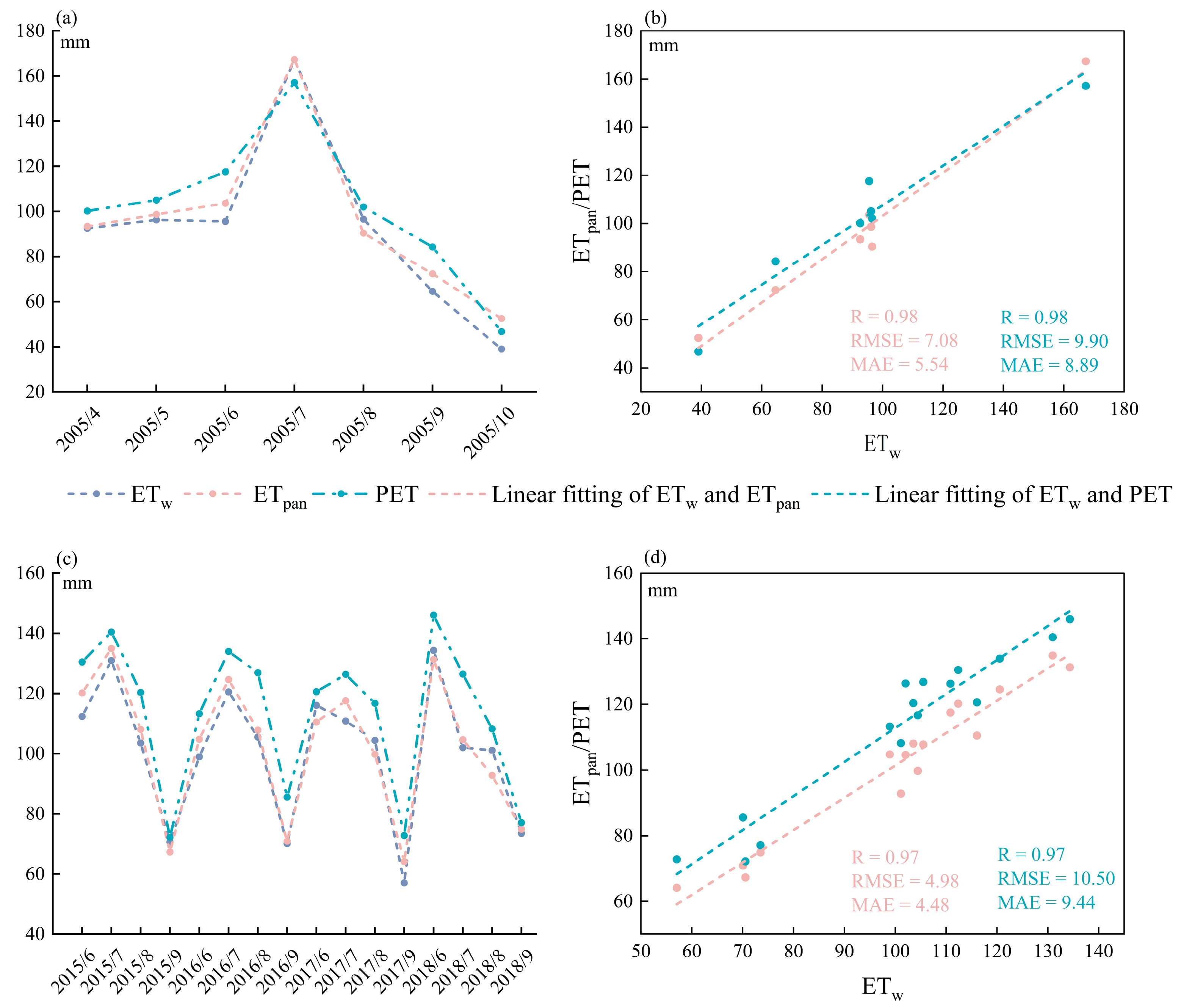
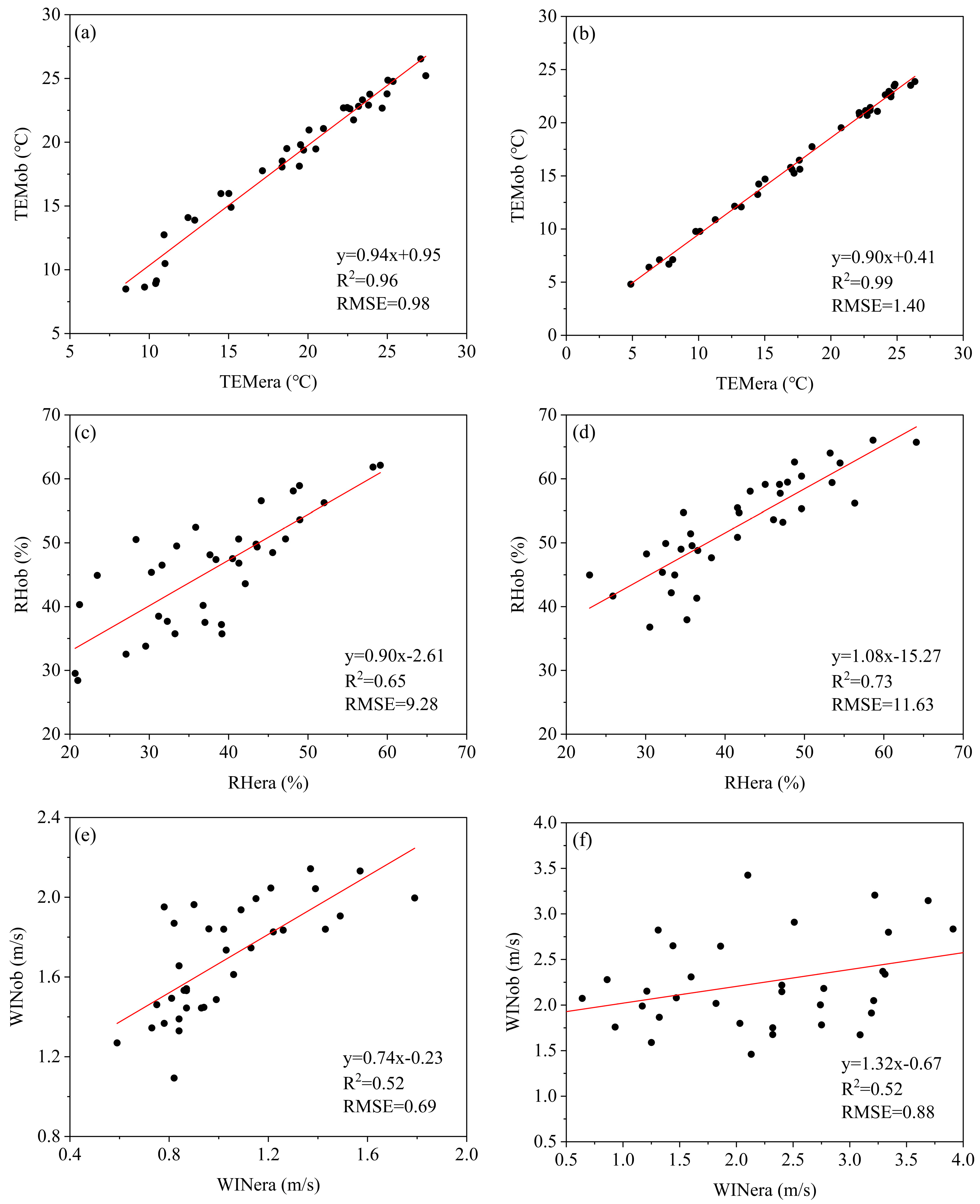
3.1. Evaluation Results of the SEBAL Model

Based on the 2021 meteorological data, the evapotranspiration (ETc) of different crop types during the growing season was calculated using the FAO Penman–Monteith method and crop coefficients. Correlation analysis was performed for the monthly ETa and ETc value sequences of each crop sample point in the study areas (Figure 2).

Table 4. Performance of the ETa and ETc correlations for different crops.

Study Area	Crop	Number of Sampling Points	Correlation			Passing Rate (>0.6)	RMSE (mm)	MAE (mm)
			>0.8	0.6~0.8	<0.6
IAY	Corn	48	31	9	8	0.83	6.78	5.83
	Pepper	122	66	19	37	0.69	8.27	7.49
	Tomato	39	16	9	14	0.64	6.88	5.77
IAB	Corn	102	96	4	2	0.98	6.11	5.14
	Sunflower	57	54	0	3	0.94	4.03	3.37
	Alfalfa	10	7	2	1	0.90	4.95	4.03

summarizes the additional statistics. In the IAY, the correlation coefficients of the corn, pepper, and tomato sampling points ranged from 0.6 to 1, especially for pepper, as 69% of the 122 pepper sampling points had correlations higher than 0.6. The RMSE of the sampling points for the three crops was within 8.5 mm, and the MAE was within 7.5 mm. In the IAB, the correlation coefficients of the corn, sunflower, and alfalfa sampling points ranged from 0.8 to 1, while the RMSE and MAE were within 6 mm. Overall, ETa fitted well with ETc. Therefore, these results indicate that the SEBAL model could efficiently estimate ETa in both study areas.

Table 5. Comparison of the ETa and ETc of several typical crops in the growth periods.

Study Area	Crop	Month	ETc (mm)	ETa (mm)
IAY	Corn	June	134.33	147.12
		July	211.74	205.85
		August	167.49	170.54
	Pepper	June	186.23	190.11
		July	186.05	196.77
		August	143.30	158.45
	Tomato	June	195.46	193.99
		July	203.18	209.27
		August	133.29	140.66
IAB	Corn	June	93.65	86.39
		July	161.15	166.68
		August	125.23	136.64
	Sunflower	May	80.76	81.08
		June	128.56	134.77
		July	89.66	81.58
	Alfalfa	June	128.22	124.52
		July	148.83	157.05
		August	156.71	150.53

compares the monthly ETa retrieved by the SEBAL model and the ETc calculated by the FAO Penman–Monteith method for typical crops in the IAY and IAB. The phenological growth stages of various crops are different. For unified comparative analysis, corn, peppers, tomatoes, and alfalfa were selected for comparison in June, July, and August, all in the same critical growth period. Since the sunflower has a shorter growth cycle, May, June, and July were chosen for comparison. The results in Table 5 indicated that the deviations between the ETa and ETc of corn, peppers, and tomatoes in the IAY were within 13 mm, 8 mm, and 15 mm, respectively. In the IAB, the deviations between the ETa and ETc of corn, sunflower, and alfalfa were within 12 mm, 8 mm, and 9 mm, respectively. The SEBAL model was generally reliable in estimating the ETa of farmland in the study areas.

The evaporation data observed from the Yanqi meteorological station from April to October 2005 and from the Burqin meteorological station from June to September 2015 to 2018 were collected to compare with the water evaporation data inverted by the SEBAL model (ETw). At the same time, the ETw was compared with the potential evapotranspiration (PET) calculated using the FAO Penman–Monteith method based on the conventional observation data from the two meteorological stations. In the Yanqi meteorological station, the errors between ETw and ETpan and between ETw and PET were within 7.08 and 10 mm, respectively (Figure 3). In the Burqin meteorological station, the errors between ETw and ETpan and between ETw and PET were within 5 and 10.5 mm, respectively. Overall, the results of the three verification methods indicated that the SEBAL model’s accuracy in estimating the evapotranspiration of typical irrigation areas in Xinjiang met regional application requirements.

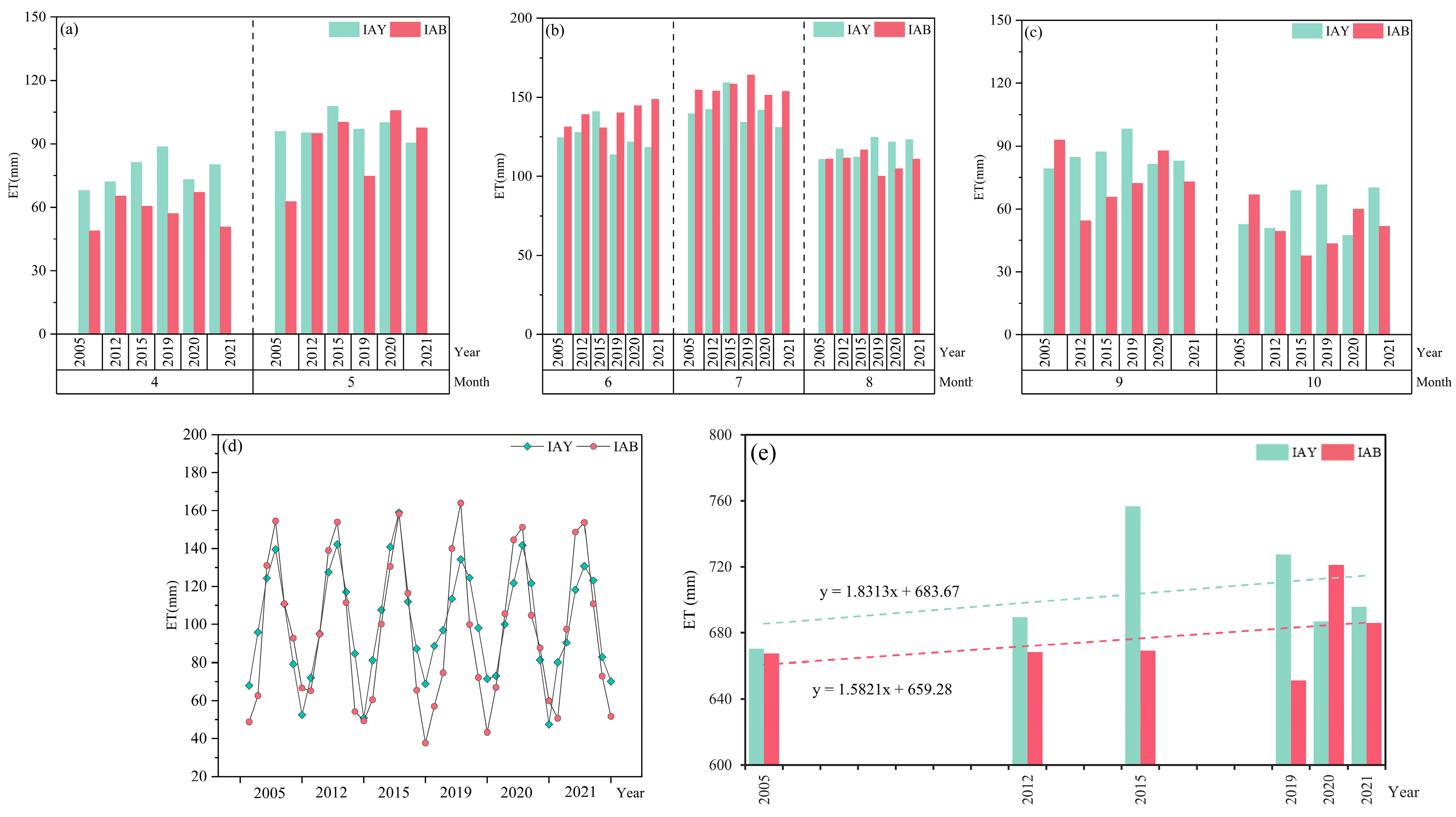
3.2. Temporal Variations in ETa

Figure 4 shows the monthly ETa for the IAY and IAB from 2005 to 2021. Regarding the monthly variation, the intra-annual trend in ETa in the two study regions was approximately the same, showing a single peak trend. Both irrigation areas had their largest ETa value in July. For the IAY, the average ETa in July ranged from 130 to 159 mm. For the IAB, the average ETa in July ranged from 151 to 164 mm. During the growing season, the overall multi-year trend showed that ETa in the two study areas increased gradually from April to May; when the temperature rose, crops began to sprout, and vegetation turned green, causing a gradual increase in ETa. ETa increased significantly from May to July when the temperature increased significantly, and the sunshine time, precipitation, and vegetation growth increased, especially in agricultural fields. The soil moisture supply was sufficient due to irrigation, resulting in high ETa. ETa decreased slightly in July and August but decreased significantly from August to October. In September and October, the climatic conditions changed significantly, with a decrease in ETa due to lower temperatures, lower net radiation, and less irrigation water for agriculture. In October, the soil began to freeze and thaw in some areas, reducing soil moisture and ETa. Regarding annual changes, the total ETa in the IAB and IAY showed fluctuating increasing trends from 2005 to 2021. The ETa in the IAY fluctuated from 670 to 756 mm, with a multi-year average of 704 mm. The ETa in the IAB fluctuated from 651 to 721 mm, with a multi-year average of 677 mm. The average annual ETa in the IAY was almost always higher than that of the IAB during the survey years.

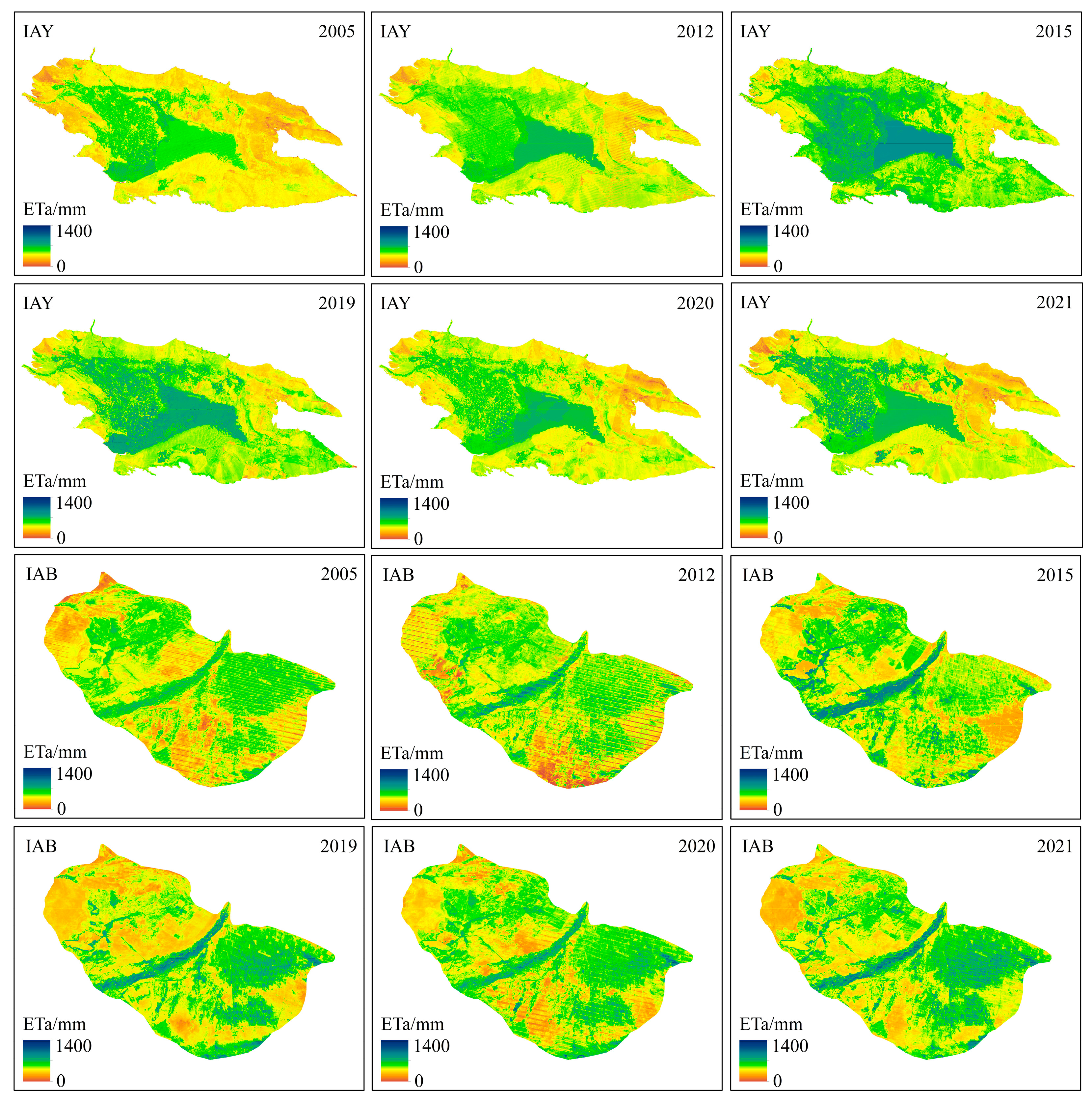
3.3. Spatial Heterogeneity of ETa

From the perspective of spatial distribution, ETa showed a decreasing distribution characteristic from the center to the surrounding areas in the IAY (Figure 5). This spatial distribution is mainly related to the land cover types. Sparsely vegetated areas and bare land dominate the margins in the IAY, while the region’s center is dominated by cropland and water bodies. Well-irrigated crops, wetlands, and water bodies showed higher ETa values due to relatively adequate water supply. In contrast, bare land and sparsely vegetated areas had lower ETa values because of high solar radiation and insufficient water supply. The IAB exhibited a greater distribution of ETa in the north than in the south, and higher ETa was mainly observed in the Burqin River and croplands near the river. The spatial distribution of ETa has remained essentially the same over the years in the IAB, with localized differences caused by changes in land cover types and cropping structure. Compared to the IAB, the spatial differentiation characteristics of ETa in the IAY were obvious. Due to the concentrated spatial distribution of cultivated land, water bodies, and bare land in the IAY, the spatial differences in ETa within the region were obvious. However, the land cover types in the IAB are evenly distributed in space, which made its ETa differ less spatially.

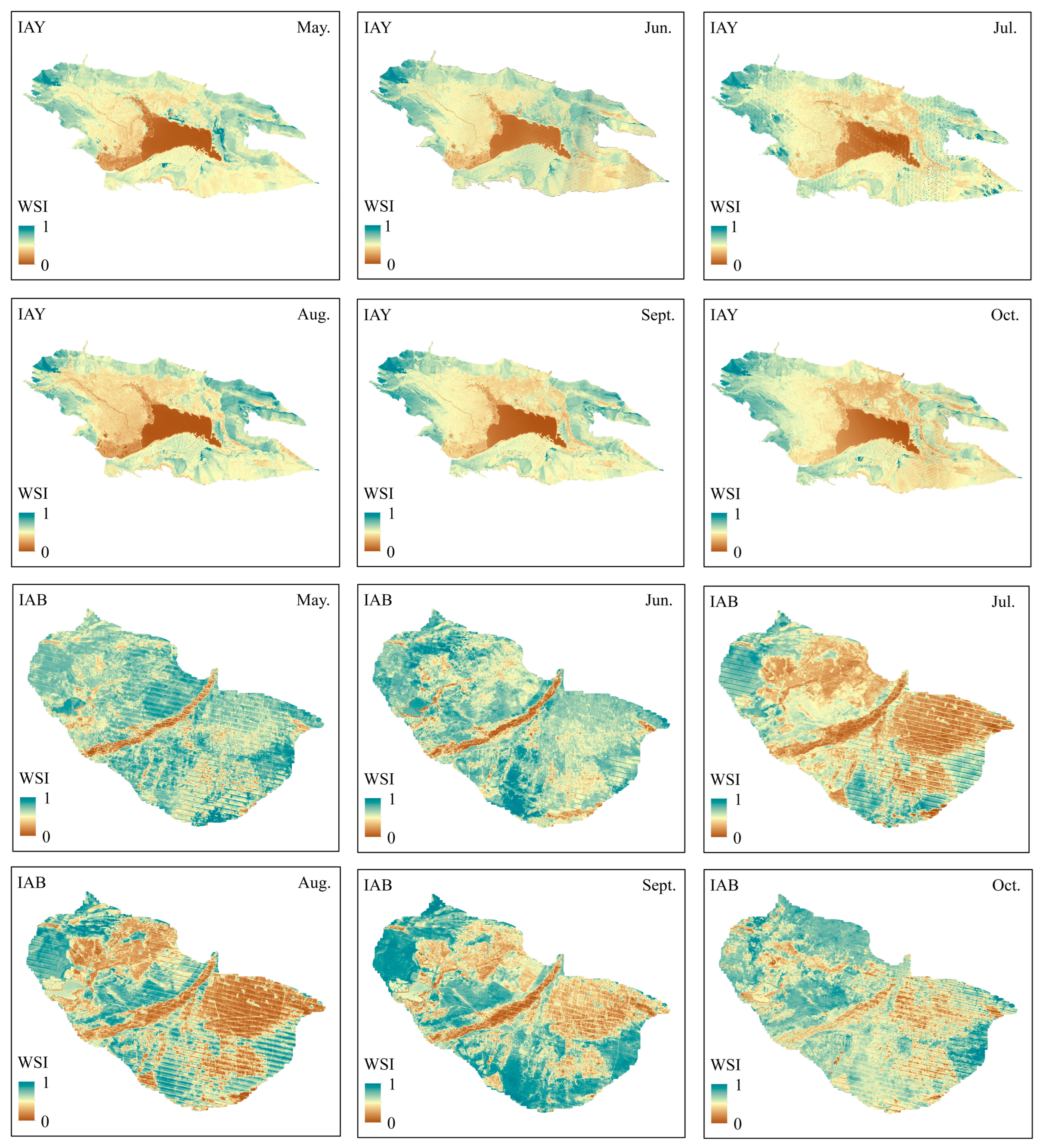
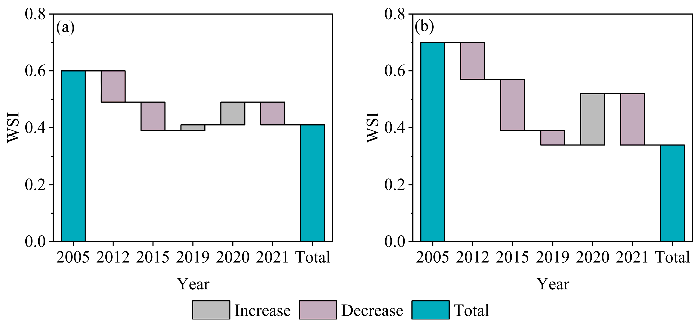
3.4. Water Stress Variation

Figure 6 shows the spatiotemporal changes in the WSI in the IAY and IAB. The results indicated that the spatial distribution of water stress in typical irrigation areas was related to land cover types. The WSI showed an increasing trend from the center to the surrounding areas in the IAY. The cultivated land and water bodies in the center of the IAY showed low levels of water stress due to relatively sufficient water supply. Deserts and the sparse vegetation areas on the edges of the IAY showed greater water stress due to insufficient water supply from the underlying surface. In the IAB, cultivated land dominated the northern part, so the WSI in the north was greater than in the south. Smaller WSI values were mainly distributed in the Burqin River area and the cultivated land near the river. In terms of spatial changes, compared to the IAB, the monthly change in the WSI was not significant in the IAY, which is mainly related to the main land use types in the irrigation areas.

In the IAB, the proportions of forestland, grassland, cultivated land, water bodies, built-up land, and bare land were 9.2%, 4.47%, 64.12%, 1.84%, 0.17%, and 20.2%, respectively. In the IAY, the proportions of forestland, grassland, cultivated land, water bodies, built-up land, and bare land were 0.2%, 4.10%, 31.25%, 13.60%, 2.14%, and 48.71%, respectively. The water stress of the water bodies changed very little, and the bare land had been in a state of insufficient water supply for a long time, so its water stress was relatively stable. Except for these land use types (water bodies and bare land) with small changes in water stress, the IAY was dominated by cultivated land and grassland with low coverage. In contrast, the IAB was dominated by cultivated land, forestland, and grassland with higher coverage. Due to irrigation and water supply, the water stress of cultivated land, forestland, and grassland would change significantly during the growing season. Therefore, the spatial variation in WSI in the IAB was obvious during the growing season. In July and August, precipitation entered a relatively abundant stage throughout the year. The supply of soil moisture in farmland was sufficient due to irrigation, so lower WSI were observed in the IAY and IAB. High water stress values were observed in some areas in May and October due to reduced precipitation and irrigation volumes.

As shown in Figure 7, the WSI showed a decreasing trend in the IAY and IAB from 2005 to 2015, decreasing by 0.21 and 0.31, respectively. From 2015 to 2021, the WSI in the IAY and IAB increased slightly, by 0.02 and 0.04, respectively. However, the WSI in the IAY and IAB showed an overall decreasing trend during the entire study period (from 2005 to 2021). In the IAY, the WSI decreased from 0.6 in 2005 to 0.41 in 2021. In the IAB, the WSI decreased from 0.7 in 2005 to 0.34 in 2021. A value of 0.2 is usually considered the minimum threshold for the WSI. According to the classification standard in Table 3, the results in

Table 6. WSI of different land cover classes in the IAY and IAB.

Study Area	Forest	Grass	Water	Farmland	Urban	Unused Land
IAY	0.51	0.48	0.11	0.38	0.40	0.56
IAB	0.58	0.57	0.14	0.47	0.56	0.67

indicate that moderate water stress dominated the land cover types except water in the two irrigation areas. The WSI of the land cover type in the IAB was higher than in the IAY, which may be related to the water-saving irrigation levels in the two irrigation areas.

4. Discussion

4.1. Accuracy Assessment of the SEBAL Model

Since the SEBAL model required input from different datasets, this study used different satellite platforms and reanalysis of climate datasets in the GEE, which might cause some errors in the inversion results of the model. Particularly in terms of reanalyzed climate data, the ERA5-Land data were downscaled using corrected thermodynamic input [47]. The meteorological data with low resolution and obtained by the simple downscaling method may have some errors when applied to the regional scale, which will cause further estimation errors for the energy fluxes. To reduce the errors in estimation results as much as possible, existing observation data from the Yanqi meteorological station and Burqin meteorological station were used to evaluate the accuracy of ERA5-Land data before applying it to evapotranspiration inversion in this study. The results indicated that the ERA5-Land data have good consistency with the observation data and the error is within an acceptable range (Figure 8). Moreover, previous studies have shown that the SEBAL model has lower sensitivity to meteorological inputs, but higher sensitivity to surface temperature and the near-surface temperature gradient [48,49]. The land surface temperature was corrected by using the DEM; the hot and cold pixels were selected through continuously adjusting the thresholds of NDVI and the land surface temperature, which could reduce the uncertainties of ETa inversion.

At the three weather stations in the IAY, evaporation from a 20 cm pan (E20) was observed from April to October 2015. Observations of the water surface evaporation from an E601 evaporator, from June to September 2015 to 2018, were collected for the IAB. However, these water surface evaporation observations were not representative of natural water evaporation, which was significantly greater. Therefore, the data observed from the evaporation pan were converted before application. For the IAY, a 0.58 conversion coefficient was used for the E20 small evaporator to calculate the actual water evaporation [50]. For the IAB, a 0.83 conversion coefficient was used for the E601 evaporator [51]. The ETa simulated by SEBAL yielded acceptable accuracy compared to the measured data in the study areas.

Several typical crops in both study areas were selected and ETa was evaluated using the ETc calculated by the FAO Penman–Monteith method and crop coefficients. For the calculation of ETc, determining the crop coefficient (${\mathrm{K}}_{\mathrm{c}}$) value is crucial. The ${\mathrm{K}}_{\mathrm{c}}$ recommended by the United Nations Food and Agriculture Organization (FAO) is based on standard conditions (adequate soil moisture). Considering the difference between field conditions in arid areas and standard conditions, the ${\mathrm{K}}_{\mathrm{c}}$ values for different crop types were adjusted according to crop characteristics and climatic conditions in the study area, and the soil water stress coefficient (${\mathrm{K}}_{\mathrm{s}}$) was also used to adjust the calculation of ETc [43]. This adjustment made the ETc closer to crop water consumption under actual environmental conditions, thereby reducing the uncertainty of the FAO Penman–Monteith method. In the IAY, the ETa errors for corn, pepper, and tomato were within 8.3 mm, among which the inversion result of corn evapotranspiration was the best, with an error within 6.78 mm. In the IAB, the ETa errors for corn, sunflower, and alfalfa were within 6.2 mm. The inversion result for sunflower evapotranspiration was the best, with an error of approximately 4 mm. The source of errors may include the effect of different soil backgrounds and random errors induced by crop sampling points.

Cha et al. [52] used the SEBAL model to estimate the crop evapotranspiration of the Kai-Kong River Basin, which covers the IAY; they found a range of 0 to 240 mm/month. Li [53] indicated that the ETa of the Bosten Lake Basin, located in the IAY, ranged from 0 to 204 mm/month. The simulated ETa from this study is consistent with those of previous studies. Generally, the above discussion indicates that the constructed SEBAL model is applicable for ETa inversion of these irrigation areas in Xinjiang, northwest China.

4.2. Driving Factors of Spatial–Temporal Changes in ETa and WSI

4.2.1. Meteorological Factors

The correlation between the monthly average ETa each year and meteorological factors was analyzed to explore the effect of climate factors on ETa. ETa was positively correlated with temperature, precipitation, relative humidity, wind speed, and sunshine hours, with correlation coefficients of 0.76, 0.31, 0.01, 0.19, and 0.16, respectively (Figure 9b). This suggested that temperature may be a critical factor influencing changes in ETa in the IAY, followed by precipitation. The IAY is located in the middle reaches of the Kai-kong River Basin. It receives limited precipitation compared to the upper reaches of mountainous areas. Precipitation increases the water content but reduces the temperature and weakens atmospheric radiation.

In the IAB, ETa was positively correlated with temperature, precipitation, and sunshine hours, with correlation coefficients of 0.9, 0.25, and 0.64, respectively (Figure 9c). This suggested that temperature was the main factor influencing changes in ETa. Relative humidity and wind speed had negative correlations with ETa, with correlation coefficients of −0.01 and −0.4, respectively. Evapotranspiration is a complex process affected by many environmental factors, among which wind speed is one of the most important. In general, wind speed can accelerate water evaporation and water vapor diffusion on the surface of plants, thus promoting evapotranspiration. However, the relationship between evapotranspiration and wind speed may show different trends in the growing season, especially in a desert oasis environment. The actual observations have found that evapotranspiration in a desert oasis may be negatively correlated with wind speed, and this correlation is small [54]. In such conditions, soil moisture status and vegetation cover have a more significant impact on evapotranspiration in the actual environment, resulting in the impact of wind speed being relatively weakened. The temperature in the IAY and IAB showed an increasing trend (Figure 9a), which was similar to the increasing trend in ETa from 2005 to 2021. Together, these results indicated that climate warming is the fundamental driving force for ETa in the IAY and IAB, and varyingly contributed to the increase in ETa from 2005 to 2021.

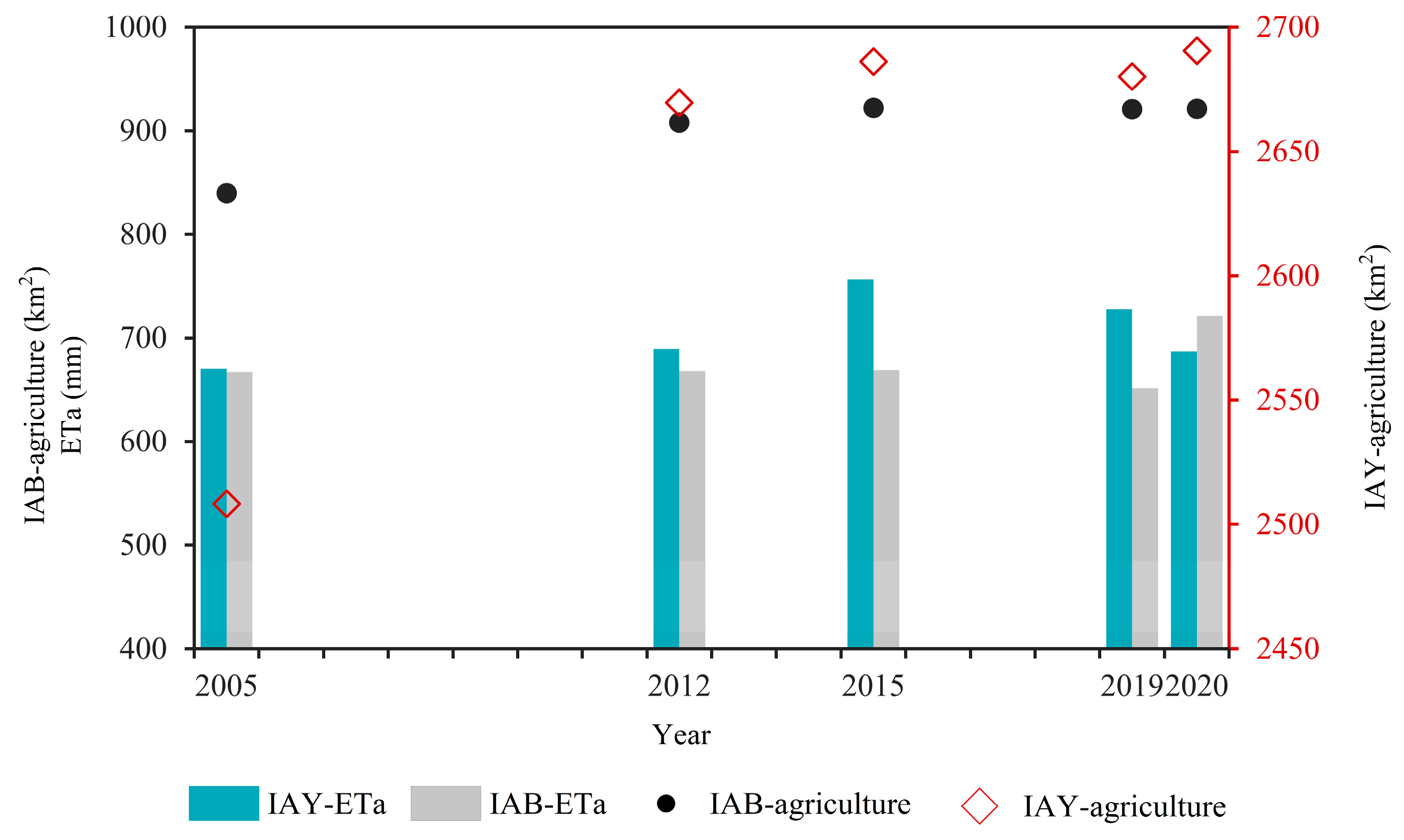
4.2.2. Regional Water Supply

In arid inland river basins, precipitation in the oasis is negligible compared to the huge water-demand gap, and irrigation has become the major source of water for consumption. The Kaidu and Burqin rivers are the main water supplies in the IAY and IAB, respectively. The Dashankou hydrological station recorded the runoff of the Kaidu River into the IAY, and the Qunkule hydrological station recorded the runoff of the Burqin River into the IAB. As shown in Figure 10a,b, the average annual runoff recorded by the Qunkule hydrological station was larger than that of the Dashankou hydrological station. The multi-year average runoffs recorded at the Dashankou hydrological station and Qunkule hydrological station were 38.37 × 10⁸ m³ and 47.67 × 10⁸ m³, respectively. In terms of monthly variation, the change in the monthly ETa corresponded with the monthly river runoff in both regions (Figure 10c,d). The discharge and ETa were lower in April and October, and the higher WSI indicated higher water stress. From May to July, as the irrigation water supply increased, the ETa increased and the WSI decreased, indicating lower water stress. The difference between monthly water consumption and surface runoff in the IAY region is smaller than in the IAB, mainly because the climate in the IAB is relatively humid and the surface runoff is greater than in the IAY. The IAY implemented joint irrigation of surface water and groundwater to meet the agricultural irrigation demand. Groundwater is an important source of the water supply in the IAY.

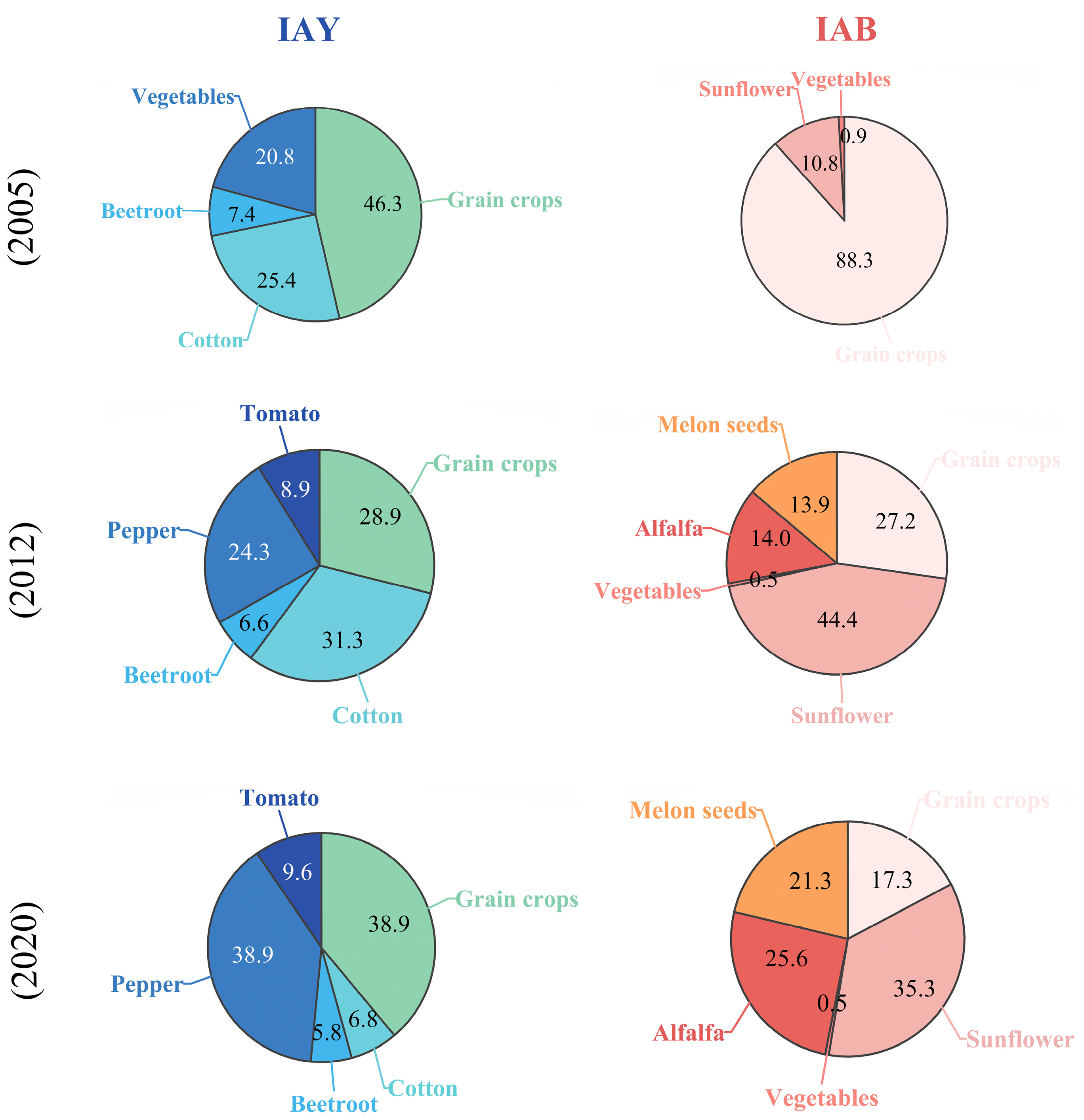
4.2.3. Irrigation Area and Planting Patterns

The agricultural land area in the IAY and IAB has expanded over the past 15 years. From 2005 to 2020, the agricultural land area increased from 2508.30 to 2690.46 km² in the IAY and from 839.79 to 921.24 km² in the IAB. The overall agricultural area in the two study areas showed a trend of rapid increase, followed by a slight decrease, and then a slow increase, consistent with the annual changes in ETa (Figure 11).

From 2005 to 2020, cash crops gradually replaced grain crops in the IAY and IAB (Figure 12). In the IAY, grain crops accounted for the largest proportion of the overall planting area in 2005, at 46.3%, followed by cotton. In 2012, the proportion for cotton (31.3%) exceeded that of grain crops (28.9%), and the proportion for cash crops (peppers and tomatoes, mainly industrial peppers and tomatoes) reached 33.2%. However, in 2020, the proportion for cash crops was the largest, followed by grain crops, while the proportion for cotton planting decreased sharply. In the IAB, from 2005 to 2012, the proportion of the planting area devoted to grain crops decreased from 88.3% to 27.2%, and that for sunflowers increased from 10.8% to 44.4%. From 2012 to 2020, the proportion of grain crop acreage continued to decrease, the proportion of sunflower acreage decreased by 9.1%, and the proportions of alfalfa and melon seeds increased by 11.6% and 7.4%, respectively. According to previous studies, the water consumption of vegetables, cotton, and oil crops is higher than that of grain crops [55,56]. Thus, agricultural water consumption in the IAY and IAB has shifted from grain crops to cash crops, which may have contributed to the increased ETa in both regions (Figure 4). The expansion of agricultural land and the changes in cropping structures had important effects on ETa in the irrigation areas.

4.2.4. Irrigation Modes

The IAY and IAB are both typical arid oasis irrigation areas in Xinjiang, northwest China, with low precipitation and high evaporation. Irrigation water is the main source of agricultural water consumption in oases. Agricultural irrigation activities have important effects on water and energy processes, such as air temperature, precipitation, and evapotranspiration [57,58]. With changes in irrigation methods and expansion of water-saving irrigation area in farmland, the process of affecting regional surface evapotranspiration becomes more complex. Before 2000, Xinjiang mainly relied on conventional irrigation methods, such as furrow-border irrigation and flood irrigation; however, after 2000, efficient water conservation technologies were implemented and promoted, including channel seepage control, sprinkler irrigation, and drip irrigation. From 2005 to 2021, the IAY and IAB developed from flood irrigation to water-saving irrigation based on drip irrigation under plastic films. In the IAY, the efficiency of flood irrigation was less than 0.4, whereas that of drip irrigation could be as high as 0.55. The proportion of drip irrigation in the four counties of the IAY ranged from 66.9% to 100% [59]. The irrigation water utilization coefficient can be used as a measure of the water-saving level [60]. In 2003, the irrigation water utilization coefficient of the IAY was 0.53 and that of the IAB was 0.38; in 2008, that of the IAY canals was 0.67 and that of the IAB canals was 0.41; in 2012, that of the IAY reached 0.58; and in 2019, that of the IAB reached 0.54. The level of water-saving irrigation in the IAY was higher than that in the IAB. Higher water-saving irrigation technologies can improve the utilization efficiency of water resources and alleviate water stress to a certain extent [61]. Therefore, the overall WSI of the IAY was smaller than that of the IAB. From 2005 to 2021, the overall decreasing trend for the WSI in the IAY and IAB was largely due to the popularization of new water-saving irrigation patterns in the two regions, which reduced ineffective evapotranspiration and had a positive impact on solving the problem of water scarcity in the basins.

With the improvements in water-saving irrigation levels in the study areas, there may be two reasons for the increases in ETa in the IAY and IAB. Firstly, when implementing water-saving irrigation on a large scale, climate warming, cultivated area expansion, and cropping pattern changes (the proportions for the food crop area and the cash crop area) have increased ETa in the IAY and IAB. Secondly, the widespread adoption of water conservation measures such as drip irrigation, and increased use of fertilizers and mulch, may have also led to the increased ETa [62]. Many factors influence the evapotranspiration process which may interact, with a change in one factor causing changes in other factors. Due to a lack of long-term series data for the irrigation areas, water-saving irrigation areas, irrigation water consumption, and water consumption for water-saving irrigation in the study areas, a more in-depth analysis cannot be carried out for the time being. In the future, when these statistical data become available, we will quantitatively analyze the impact of irrigation patterns on regional evapotranspiration and water stress in the study areas.

5. Conclusions

In this study, we built a SEBAL model based on the GEE platform to estimate the ETa of two typical irrigation areas in Xinjiang, northwest China, from 2005 to 2021. The WSI was estimated based on the simulated ETa. The monthly ETa values were consistent with the ETc calculated through the FAO Penman–Monteith method, with correlation coefficients of 0.8 or more for most sample points. The overall increasing trend in ETa in the IAY and IAB from 2005 to 2021 was mainly related to an increase in temperature, expansion of cropland, and adjustments to the cropping patterns. The WSI in the IAY was lower than that in the IAB, reflecting regional differences in water-saving technologies. The water stress in the two irrigation areas decreased from 2005 to 2021. As Xinjiang has vigorously promoted high-efficiency water-saving technologies in the past 20 years, the irrigation mode is based on under-membrane drip irrigation. The increased use of water-saving irrigation technologies has alleviated the water resource stress in the two irrigation areas.

References

1. UN. World Water Development Report. 2020. Available online: https://www.unwater.org/publications/un-world-water-development-report-2020 (accessed on 21 March 2020).
2. Liu, J.; Yang, H.; Gosling, S.N.; Kummu, M.; Flörke, M.; Pfister, S.; Hanasaki, N.; Wada, Y.; Zhang, X.; Zheng, C. Water scarcity assessments in the past, present, and future. Earth’s Future 2017, 5, 545–559. [Google Scholar] [CrossRef] [PubMed]
3. Oki, T.; Kanae, S. Global hydrological cycles and world water resources. Science 2006, 313, 1068–1072. [Google Scholar] [CrossRef] [PubMed]
4. Liu, M.; Tang, R.; Li, Z.-L.; Yan, G. Integration of two semi-physical models of terrestrial evapotranspiration using the China Meteorological Forcing Dataset. Int. J. Remote Sens. 2019, 40, 1966–1980. [Google Scholar] [CrossRef]
5. Schewe, J.; Heinke, J.; Gerten, D.; Haddeland, I.; Arnell, N.W.; Clark, D.B.; Dankers, R.; Eisner, S.; Fekete, B.M.; Colón-González, F.J. Multimodel assessment of water scarcity under climate change. Proc. Natl. Acad. Sci. USA 2014, 111, 3245–3250. [Google Scholar] [CrossRef]
6. Sun, H.; Chen, J.; Yang, Y.; Yan, D.; Xue, J.; Wang, J.; Zhang, W. Assessment of long-term water stress for ecosystems across China using the maximum entropy production theory-based evapotranspiration product. J. Clean. Prod. 2022, 349, 131414. [Google Scholar] [CrossRef]
7. Jiang, L.; Bao, A.; Yuan, Y.; Zheng, G.; Guo, H.; Yu, T.; De Maeyer, P. The effects of water stress on croplands in the Aral Sea basin. J. Clean. Prod. 2020, 254, 120114. [Google Scholar] [CrossRef]
8. Jahangir, M.H.; Arast, M. Remote sensing products for predicting actual evapotranspiration and water stress footprints under different land cover. J. Clean. Prod. 2020, 266, 121818. [Google Scholar] [CrossRef]
9. Duan, Z.; Bastiaanssen, W. Evaluation of three energy balance-based evaporation models for estimating monthly evaporation for five lakes using derived heat storage changes from a hysteresis model. Res. Lett. 2017, 12, 024005. [Google Scholar] [CrossRef]
10. Liu, S.; Xu, Z.; Song, L.; Zhao, Q.; Ge, Y.; Xu, T.; Ma, Y.; Zhu, Z.; Jia, Z.; Zhang, F. Upscaling evapotranspiration measurements from multi-site to the satellite pixel scale over heterogeneous land surfaces. Agric. For. Meteorol. 2016, 230, 97–113. [Google Scholar] [CrossRef]
11. Liou, Y.-A.; Kar, S.K. Evapotranspiration estimation with remote sensing and various surface energy balance algorithms—A review. Energies 2014, 7, 2821–2849. [Google Scholar] [CrossRef]
12. Liu, Z.; Huang, Y.; Liu, T.; Li, J.; Xing, W.; Akmalov, S.; Peng, J.; Pan, X.; Guo, C.; Duan, Y. Water balance analysis based on a quantitative evapotranspiration inversion in the Nukus irrigation area, Lower Amu River Basin. Remote Sens. 2020, 12, 2317. [Google Scholar] [CrossRef]
13. Wang, K.; Dickinson, R.E.; Wild, M.; Liang, S. Evidence for decadal variation in global terrestrial evapotranspiration between 1982 and 2002: 1. Model development. J. Geophys. Res. Atmos. 2010, 115. [Google Scholar] [CrossRef]
14. Yao, Y.; Di, Z.; Xie, Z.; Xiao, Z.; Jia, K.; Zhang, X.; Shang, K.; Yang, J.; Bei, X.; Guo, X. Simplified priestley–taylor model to estimate land-surface latent heat of evapotranspiration from incident shortwave radiation, satellite vegetation index, and air relative humidity. Remote Sens. 2021, 13, 902. [Google Scholar] [CrossRef]
15. Yao, Y.; Liang, S.; Li, X.; Chen, J.; Wang, K.; Jia, K.; Cheng, J.; Jiang, B.; Fisher, J.B.; Mu, Q. A satellite-based hybrid algorithm to determine the Priestley–Taylor parameter for global terrestrial latent heat flux estimation across multiple biomes. Remote Sens. Environ. 2015, 165, 216–233. [Google Scholar] [CrossRef]
16. Bai, Y.; Zhang, S.; Bhattarai, N.; Mallick, K.; Liu, Q.; Tang, L.; Im, J.; Guo, L.; Zhang, J. On the use of machine learning based ensemble approaches to improve evapotranspiration estimates from croplands across a wide environmental gradient. Agric. For. Meteorol. 2021, 298, 108308. [Google Scholar] [CrossRef]
17. Carter, C.; Liang, S. Evaluation of ten machine learning methods for estimating terrestrial evapotranspiration from remote sensing. Int. J. Appl. Earth Obs. Geoinf. 2019, 78, 86–92. [Google Scholar] [CrossRef]
18. Shiri, J. Improving the performance of the mass transfer-based reference evapotranspiration estimation approaches through a coupled wavelet-random forest methodology. J. Hydrol. 2018, 561, 737–750. [Google Scholar] [CrossRef]
19. Xu, T.; Guo, Z.; Liu, S.; He, X.; Meng, Y.; Xu, Z.; Xia, Y.; Xiao, J.; Zhang, Y.; Ma, Y. Evaluating different machine learning methods for upscaling evapotranspiration from flux towers to the regional scale. J. Geophys. Res. Atmos. 2018, 123, 8674–8690. [Google Scholar] [CrossRef]
20. Chen, Y.; Yuan, W.; Xia, J.; Fisher, J.B.; Dong, W.; Zhang, X.; Liang, S.; Ye, A.; Cai, W.; Feng, J. Using Bayesian model averaging to estimate terrestrial evapotranspiration in China. J. Hydrol. 2015, 528, 537–549. [Google Scholar] [CrossRef]
21. Yang, Y.; Sun, H.; Xue, J.; Liu, Y.; Liu, L.; Yan, D.; Gui, D. Estimating evapotranspiration by coupling Bayesian model averaging methods with machine learning algorithms. Environ. Monit. Assess. 2021, 193, 156. [Google Scholar] [CrossRef]
22. Yuan, Q.; Shen, H.; Li, T.; Li, Z.; Li, S.; Jiang, Y.; Xu, H.; Tan, W.; Yang, Q.; Wang, J. Deep learning in environmental remote sensing: Achievements and challenges. Remote Sens. Environ. 2020, 241, 111716. [Google Scholar] [CrossRef]
23. Long, D.; Singh, V.P. A two-source trapezoid model for evapotranspiration (TTME) from satellite imagery. Remote Sens. Environ. 2012, 121, 370–388. [Google Scholar] [CrossRef]
24. Tang, R.; Li, Z.-L.; Tang, B. An application of the Ts–VI triangle method with enhanced edges determination for evapotranspiration estimation from MODIS data in arid and semi-arid regions: Implementation and validation. Remote Sens. Environ. 2010, 114, 540–551. [Google Scholar] [CrossRef]
25. Wu, B.; Yan, N.; Xiong, J.; Bastiaanssen, W.; Zhu, W.; Stein, A. Validation of ETWatch using field measurements at diverse landscapes: A case study in Hai Basin of China. J. Hydrol. 2012, 436, 67–80. [Google Scholar] [CrossRef]
26. Zhang, Y.; Kong, D.; Gan, R.; Chiew, F.H.; McVicar, T.R.; Zhang, Q.; Yang, Y. Coupled estimation of 500 m and 8-day resolution global evapotranspiration and gross primary production in 2002–2017. Remote Sens. Environ. 2019, 222, 165–182. [Google Scholar] [CrossRef]
27. Allen, R.G.; Tasumi, M.; Trezza, R. Satellite-based energy balance for mapping evapotranspiration with internalized calibration (METRIC)—Model. J. Irrig. Drain. Eng. 2007, 133, 380–394. [Google Scholar] [CrossRef]
28. Qiu, G.Y.; Li, C.; Yan, C. Characteristics of soil evaporation, plant transpiration and water budget of Nitraria dune in the arid Northwest China. Agric. For. Meteorol. 2015, 203, 107–117. [Google Scholar] [CrossRef]
29. Song, L.; Kustas, W.P.; Liu, S.; Colaizzi, P.D.; Nieto, H.; Xu, Z.; Ma, Y.; Li, M.; Xu, T.; Agam, N. Applications of a thermal-based two-source energy balance model using Priestley-Taylor approach for surface temperature partitioning under advective conditions. J. Hydrol. 2016, 540, 574–587. [Google Scholar] [CrossRef]
30. Cheng, M.; Jiao, X.; Li, B.; Yu, X.; Shao, M.; Jin, X. Long time series of daily evapotranspiration in China based on the SEBAL model and multisource images and validation. Earth Syst. Sci. Data 2021, 13, 3995–4017. [Google Scholar] [CrossRef]
31. De Lima, C.E.S.; De Oliveira Costa, V.S.; Galvíncio, J.D.; Da Silva, R.M.; Santos, C.A.G. Assessment of automated evapotranspiration estimates obtained using the GP-SEBAL algorithm for dry forest vegetation (Caatinga) and agricultural areas in the Brazilian semiarid region. Agric. Water Manag. 2021, 250, 106863. [Google Scholar] [CrossRef]
32. Liu, Z.; Liu, T.; Huang, Y.; Duan, Y.; Pan, X.; Wang, W. Comparison of crop evapotranspiration and water productivity of typical delta irrigation areas in Aral Sea Basin. Remote Sens. 2022, 14, 249. [Google Scholar] [CrossRef]
33. Taheri, M.; Emadzadeh, M.; Gholizadeh, M.; Tajrishi, M.; Ahmadi, M.; Moradi, M. Investigating the temporal and spatial variations of water consumption in Urmia Lake River Basin considering the climate and anthropogenic effects on the agriculture in the basin. Agric. Water Manag. 2019, 213, 782–791. [Google Scholar] [CrossRef]
34. Yang, L.; Li, J.; Sun, Z.; Liu, J.; Yang, Y.; Li, T. Daily actual evapotranspiration estimation of different land use types based on SEBAL model in the agro-pastoral ecotone of northwest China. PLoS ONE 2022, 17, e0265138. [Google Scholar] [CrossRef] [PubMed]
35. Senay, G.B.; Friedrichs, M.; Morton, C.; Parrish, G.E.; Schauer, M.; Khand, K.; Kagone, S.; Boiko, O.; Huntington, J. Mapping actual evapotranspiration using Landsat for the conterminous United States: Google Earth Engine implementation and assessment of the SSEBop model. Remote Sens. Environ. 2022, 275, 113011. [Google Scholar] [CrossRef]
36. Teluguntla, P.; Thenkabail, P.S.; Oliphant, A.; Xiong, J.; Gumma, M.K.; Congalton, R.G.; Yadav, K.; Huete, A. A 30-m landsat-derived cropland extent product of Australia and China using random forest machine learning algorithm on Google Earth Engine cloud computing platform. ISPRS J. Photogramm. Remote Sens. 2018, 144, 325–340. [Google Scholar] [CrossRef]
37. Gorelick, N.; Hancher, M.; Dixon, M.; Ilyushchenko, S.; Thau, D.; Moore, R. Google Earth Engine: Planetary-scale geospatial analysis for everyone. Remote Sens. Environ. 2017, 202, 18–27. [Google Scholar] [CrossRef]
38. Liaqat, U.W.; Choi, M. Accuracy comparison of remotely sensed evapotranspiration products and their associated water stress footprints under different land cover types in Korean peninsula. J. Clean. Prod. 2017, 155, 93–104. [Google Scholar] [CrossRef]
39. Yao, Y.; Mallik, A.U. Estimation of actual evapotranspiration and water stress in the Lijiang River Basin, China using a modified Operational Simplified Surface Energy Balance (SSEBop) model. J. Hydro-Environ. Res. 2022, 41, 1–11. [Google Scholar] [CrossRef]
40. Bastiaanssen, W.G.; Menenti, M.; Feddes, R.; Holtslag, A. A remote sensing surface energy balance algorithm for land (SEBAL). 1. Formulation. J. Hydrol. 1998, 212, 198–212. [Google Scholar] [CrossRef]
41. Losgedaragh, S.Z.; Rahimzadegan, M. Evaluation of SEBS, SEBAL, and METRIC models in estimation of the evaporation from the freshwater lakes (Case study: Amirkabir dam, Iran). J. Hydrol. 2018, 561, 523–531. [Google Scholar] [CrossRef]
42. Allen, R.; Tasumi, M.; Trezza, R.S.; Bastiaanssen, W. Surface Energy Balance Algorithm for Land: Advanced Training and Users Manual; University of Idaho: Moscow, ID, USA, 2002; pp. 1–98. [Google Scholar]
43. Allen, R.G.; Pereira, L.S.; Raes, D.; Smith, M. Crop Evapotranspiration—Guidelines for Computing Crop Water Requirements—FAO Irrigation and Drainage Paper 56; FAO: Rome, Italy, 1998; Volume 300, p. D05109. [Google Scholar]
44. Zhang, Y.; Wegehenkel, M. Integration of MODIS data into a simple model for the spatial distributed simulation of soil water content and evapotranspiration. Remote Sens. Environ. 2006, 104, 393–408. [Google Scholar] [CrossRef]
45. Liao, J.; Lei, B.; Su, T.; Liu, W.; Zhang, W.; Zhu, F. Prediction of winter wheat water demand based on remote sensing modified crop coefficient. Water Sav. Irrig. 2023, 3, 48–52,60. [Google Scholar]
46. Quan, Z.; Zuo, Q.; Wang, P.; Zhang, Y. Ecological vulnerability analysis of the Qin River basin based on SWAT and water stress index. J. North China Univ. Water Resour. Electr. Power (Nat. Sci. Ed.) 2024, 45, 15–24. [Google Scholar]
47. Muñoz-Sabater, J.; Dutra, E.; Agustí-Panareda, A.; Albergel, C.; Arduini, G.; Balsamo, G.; Boussetta, S.; Choulga, M.; Harrigan, S.; Hersbach, H. ERA5-Land: A state-of-the-art global reanalysis dataset for land applications. Earth Syst. Sci. Data 2021, 13, 4349–4383. [Google Scholar] [CrossRef]
48. Biggs, T.W.; Marshall, M.; Messina, A. Mapping daily and seasonal evapotranspiration from irrigated crops using global climate grids and satellite imagery: Automation and methods comparison. Water Resour. Res. 2016, 52, 7311–7326. [Google Scholar] [CrossRef]
49. Laipelt, L.; Ruhoff, A.L.; Fleischmann, A.S.; Kayser, R.H.B.; Kich, E.d.M.; da Rocha, H.R.; Neale, C.M.U. Assessment of an automated calibration of the SEBAL algorithm to estimate dry-season surface-energy partitioning in a forest–savanna transition in Brazil. Remote Sens. 2020, 12, 1108. [Google Scholar] [CrossRef]
50. Yang, Y. Study on Water Balance in Kaidu-Kongqi River Basin Using Remote-Sensing Data. Master’s Thesis, China University of Geosciences (Beijing), Beijing, China, 2021. [Google Scholar]
51. Shi, C.; Niu, K.; Chen, T.; Zhu, X. The study of pan coefficients of evaporation pans of water. Sci. Geogr. Sin. 1986, 6, 305–313. [Google Scholar]
52. Cha, M.; Li, M.; Wang, X. Estimation of Seasonal Evapotranspiration for Crops in Arid Regions Using Multisource Remote Sensing Images. Remote Sens. 2020, 12, 2398. [Google Scholar] [CrossRef]
53. Li, Z. Analysis of Evapotranspiration Change in the Arid Region of Northwest China. Ph.D. Thesis, Xinjiang Institute of Ecology and Geography Chinese Academy of Sciences, Ürümqi, China, 2014. [Google Scholar]
54. He, H.; Jin, X.; Hao, M.; Lang, J.; Zhang, X. Temporal-spatial distribution characteristics of evapotranspiration and its influencing factors in Tarim basin. Water Resour. Hydropower Eng. 2023, 54, 60–74. [Google Scholar]
55. Han, J. A Study on the Influential Factors of Water Requirement of Crops in Hexi Region and the Optimal Distribution of Water Resources. Ph.D. Thesis, Lanzhou University, Lanzhou, China, 2017. [Google Scholar]
56. Meng, J.; Yao, X.; Yang, X.; Luo, J.; Shen, Y. Spatial and Temporal Evolution of Agricultural Planting Structure and Crop Water Consumption in Groundwater Overdraft Area. Trans. Chin. Soc. Agric. Mach. 2020, 51, 302–312. [Google Scholar]
57. Pan, S.; Pan, N.; Tian, H.; Friedlingstein, P.; Sitch, S.; Shi, H.; Arora, V.K.; Haverd, V.; Jain, A.K.; Kato, E. Evaluation of global terrestrial evapotranspiration using state-of-the-art approaches in remote sensing, machine learning and land surface modeling. Hydrol. Earth Syst. Sci. 2020, 24, 1485–1509. [Google Scholar] [CrossRef]
58. McDermid, S.; Nocco, M.; Lawston-Parker, P.; Keune, J.; Pokhrel, Y.; Jain, M.; Jägermeyr, J.; Brocca, L.; Massari, C.; Jones, A.D. Irrigation in the Earth system. Nat. Rev. Earth Environ. 2023, 4, 435–453. [Google Scholar] [CrossRef]
59. Peng, J. Environmental Flows Assessment and Regulation of Bosten Lake Wetland. Ph.D. Thesis, Xinjiang Institute of Ecology and Geography Chinese Academy of Sciences, Ürümqi, China, 2022. [Google Scholar]
60. Zou, M.; Niu, J.; Kang, S.; Li, X.; Lu, H. The contribution of human agricultural activities to increasing evapotranspiration is significantly greater than climate change effect over Heihe agricultural region. Sci. Rep. 2017, 7, 8805. [Google Scholar] [CrossRef] [PubMed]
61. Deng, M.; Wang, Q.; Tao, W.; Wang, Z.; Cao, J. Development Model for Improving the Quality and Efficiency of Modern Agriculture in the Arid Region of Northwest China. Strateg. Study CAE 2023, 25, 59–72. [Google Scholar] [CrossRef]
62. Ding, R.; Kang, S.; Zhang, Y.; Hao, X.; Tong, L.; Du, T. Partitioning evapotranspiration into soil evaporation and transpiration using a modified dual crop coefficient model in irrigated maize field with ground-mulching. Agric. Water Manag. 2013, 127, 85–96. [Google Scholar] [CrossRef]
Figure 1. Maps of the study areas (map content approval number: GS (2019)1822). (a): The location of Xinjiang in China; (b) the location of the IAY and IAB in Xinjiang; (c) an overview of the IAY; and (d) an overview of the IAB. Note: the IAY is the irrigation area of the Yanqi Basin and the IAB is the irrigation area of Burqin.
Remotesensing 16 02676 g001
Figure 2. The ETa and ETc correlation coefficients in (a) the IAY and (b) the IAB. Note: the correlation coefficient of each sampling point is marked as a small dot and classified by crop type. ETa is the actual evapotranspiration inverted by the SEBAL model. ETc is the crop evapotranspiration calculated using the FAO Penman–Monteith method and crop coefficients.
Remotesensing 16 02676 g002
Figure 3. Comparison of ETw with ETpan and PET at the Yanqi meteorological station (a,b) and Burqin meteorological station (c,d). Note: ETw is water evaporation inverted by the SEBAL model; ETpan is converted evaporation observation data; PET is potential evapotranspiration.
Remotesensing 16 02676 g003
Figure 4. Simulation results for the monthly ETa during the growing season (ad) and the annual ETa (e) from 2005 to 2021 in the IAY and IAB.
Remotesensing 16 02676 g004
Figure 5. Spatiotemporal variations in ETa during the growing season from 2005 to 2021 in the IAY and IAB.
Remotesensing 16 02676 g005
Figure 6. Spatiotemporal variations in the WSI during the growing season from 2005 to 2021 in the IAY and IAB. Note: WSI is the water stress index.
Remotesensing 16 02676 g006
Figure 7. WSI from 2005 to 2021 in the IAY (a) and IAB (b).
Remotesensing 16 02676 g007
Figure 8. Verification results of ERA5-Land data. The vertical axis represents the monthly observation data from the meteorological station, and the horizontal axis represents the ERA5-Land monthly data: (a,c,e) for the IAY and (b,d,f) for the IAB. Note: TEM is temperature; RH is relative humidity (RHera is calculated by the dew-point temperature at 2 m of ERA5-Land); and WIN is wind speed (WINera is calculated by the eastward and northward components of 10 m wind speed of ERA5-Land).
Remotesensing 16 02676 g008
Figure 9. Average temperature for the year and growing season (a) and correlation coefficients between ETa and meteorological factors in the IAY (b) and IAB (c). Note: in the IAY, the meteorological data are from the Yanqi, Hejing, and Heshuo stations; in the IAB, the meteorological data are from the Burqin station. TEM is temperature; PRE is precipitation; RHU is relative humidity; WIN is wind speed; and SSD is sunshine hours.
Remotesensing 16 02676 g009
Figure 10. Annual runoff variation trend for the Dashankou (a) and Qunkule (b) hydrological stations from 2000 to 2018. Intra-annual variation trend for the runoff, ETa, and WSI for the IAY (c) and IAB (d).
Remotesensing 16 02676 g010
Figure 11. Agriculture land area and ETa variation in the IAY and IAB from 2005 to 2020.
Remotesensing 16 02676 g011
Figure 12. Main crop-type proportions in the IAY and IAB.
Remotesensing 16 02676 g012