Precise Motion Compensation of Multi-Rotor UAV-Borne SAR Based on Improved PTA

Abstract

In recent years, with the miniaturization of high-precision position and orientation systems (POS), precise motion errors during SAR data collection can be calculated based on high-precision POS. However, compensating for these errors remains a significant challenge for multi-rotor UAV-borne SAR systems. Compared with large aircrafts, multi-rotor UAVs are lighter, slower, have more complex flight trajectories, and have larger squint angles, which result in significant differences in motion errors between building targets and ground targets. If the motion compensation is based on ground elevation, the motion error of the ground target will be fully compensated, but the building target will still have a large residual error; as a result, although the ground targets can be well-focused, the building targets may be severely defocused. Therefore, it is necessary to further compensate for the residual motion error of building targets based on the actual elevation on the SAR image. However, uncompensated errors will affect the time–frequency relationship; furthermore, the ω-k algorithm will further change these errors, resulting in errors in SAR images becoming even more complex and difficult to compensate for. To solve this problem, this paper proposes a novel improved precise topography and aperture-dependent (PTA) method that can precisely compensate for motion errors in the UAV-borne SAR system. After motion compensation and imaging processing based on ground elevation, a secondary focus is applied to defocused buildings. The improved PTA fully considers the coupling of the residual error with the time–frequency relationship and ω-k algorithm, and the precise errors in the two-dimensional frequency domain are determined through numerical calculations without any approximations. Simulation and actual data processing verify the effectiveness of the method, and the experimental results show that the proposed method in this paper is better than the traditional method.

1. Introduction

Motion compensation is crucial for multi-rotor UAV-borne SAR [1] imaging, with algorithms divided into those based on a POS and those based on echo data [2]. Echo data-based motion compensation, also known as autofocus algorithms, are often used when the accuracy of a POS is insufficient. These algorithms estimate and compensate for phase errors to enhance image quality. Recently, many effective autofocus algorithms have been introduced [3,4,5]. However, these methods typically involve approximations in their derivations, such as neglecting the impact of errors on stationary phase points, which means the models they create may not be sufficiently accurate. Additionally, these methods often have specific requirements for the scene. For example, Zhang et al. [6] proposed an autofocus method for a highly squinted UAV SAR, which relies on the phase gradient autofocus (PGA) algorithm, necessitating a scene with numerous prominent points. Brancato et al. [7] proposed an error estimation method suitable for repeat-pass SAR data. However, its performance is limited when the interferograms are severely affected by decorrelation.

POS-based motion compensation is more versatile, but it requires high accuracy from the POS. Different from the autofocus algorithm, the POS-based motion compensation algorithm calculates the error based on the POS and pays more attention to accurately compensating the motion error. In order to compensate for more errors before the imaging process, Meng et al. [8,9]. proposed the one-step motion compensation algorithm (OSA). This algorithm corrects the envelope error by interpolation and then compensates for the phase error, thereby compensating for the range-varying motion error before imaging. However, due to the spatial variation in the motion error, there will still be some residual errors after one-step motion compensation. The magnitude of these residual errors is related to factors such as the target’s elevation and the squint angle. If the residual errors are large enough, the image may still become defocused even after motion compensation has been applied. Therefore, the current focus of research on POS-based motion compensation is on how to precisely compensate for residual errors [10,11].

In recent years, with the miniaturization of high-precision POSs, multi-rotor UAVs have also begun to be equipped with high-precision POSs, which makes it possible to obtain well-focused SAR images based on POS-based motion compensation. However, compared with large UAVs, the residual error of the multi-rotor UAV-borne SAR system after one step motion compensation is often larger and more difficult to compensate for. This is because multi-rotor UAV-borne SAR systems, being lighter and slower, are more susceptible to atmospheric turbulence. Their flight trajectories are often more complex than those of a larger aircraft, and they tend to have larger squint angles during flight. Furthermore, due to the low flight height of multi-rotor UAVs and the presence of squint angles, the impact of target heights on motion errors becomes very significant [12]. This leads to large discrepancies in motion errors between ground and building targets in one scene. Although we can calculate the error for each target using high-precision POSs, it is not possible to uniformly compensate for them before range cell migration correction (RCMC). If motion compensation is based on ground elevation, there will still be large residual errors for building targets, and building targets will be severely defocused. Therefore, further motion compensation combined with elevation is very necessary.

The terrain and aperture-dependent motion compensation algorithm (PTA) [13,14,15] is a classic motion compensation algorithm combined with elevation. However, on the one hand, the PTA calculates the form of the residual error in the azimuthal frequency domain based on the ideal time–frequency relationship, neglecting the effect of the residual motion error on the time–frequency relationship, and on the other hand, the PTA does not consider the impact of imaging algorithms. In response to the first problem, some researchers proposed an improved PTA [16,17,18]; these improved PTAs consider the impact of the residual error on the azimuthal time–frequency stationary phase points. However, there are some approximate calculations in these methods, and these methods do not consider the effect of ω-k processing; so, they make it difficult to effectively improve the quality of multi-rotor UAV-borne SAR images.

The chirp modulated back-projection (CMBP) approach [19,20] is a high-precision motion compensation algorithm and it also can be combined with elevation. This algorithm takes into account the influence of ω-k processing on the residual error. This algorithm adds chirp signal modulation in the two-dimensional frequency domain of the image processed using the ω-k algorithm, and then two-dimensional IFFT is performed, so that the image is restored to echo data with a virtual aperture, which is much smaller than the original aperture; the aperture is then focused by the back-projection (BP) approach [21] to obtain the final well-focused SAR image. This algorithm is more efficient than the traditional BP approach due to the smaller virtual aperture, and it is more accurate and has better focus quality compared to the PTA. However, the algorithm still has a small amount of approximation in the process of deriving the two-dimensional frequency domain error, which will reduce the compensation accuracy and damage the image quality.

To more precisely compensate for residual errors in multi-rotor UAV-borne SAR images and achieve the refocusing of building targets, this paper proposes an improved PTA. This method has the advantages of simple calculation and no approximation; so, it can be used to compensate for residual errors with high accuracy. This paper provides detailed derivations and calculation methods and validates the effectiveness of this approach through simulations and real data processing.

2. Materials and Methods

2.1. Principle of Motion Compensation

The geometry of the multi-rotor UAV-borne SAR system is shown in Figure 1. The reference elevation is 0 m, $P_{real}$ is the actual position of the point target on the building and the elevation is H m, and $P_{MoCo}$ is the target located on the reference plane and at the center of the beam. The OSA is used for MOCO. According to the center-beam approximation (CBA) [22], the motion error will be calculated based on $P_{MoCo}$ to compensate for motion errors of the targets at the same slant range in the whole beam. For $P_{real}$, the residual error is caused by the deviation from the beam center in the horizontal direction and the deviation from the reference plane in the height direction, and the residual motion error ΔR after MOCO can be written as follows:

$$\mathsf{\Delta }R=R_{real}-R_{ideal}-\left(R_{real}^{MoCo}-R_{ideal}^{MoCo}\right)$$

(1)

Due to the low flight altitude of the multi-rotor UAV and the squint angles, for targets located on the ground, the ΔR may be so small that the impact on imaging can be neglected. However, for targets located on the rooftop of buildings, the ΔR could be large, resulting in severe defocusing after imaging.

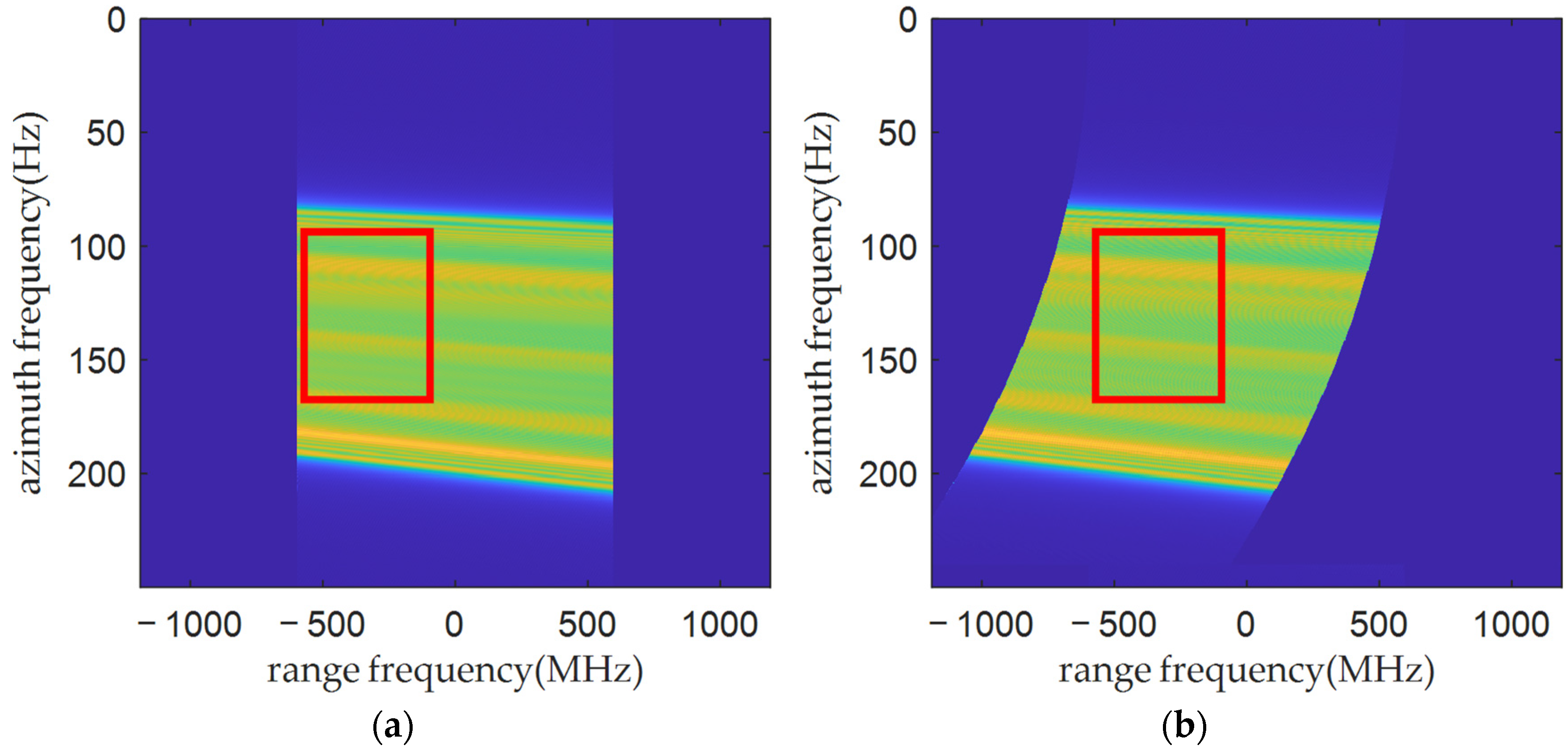
2.2. Spectrum of Signal with Errors

The two-dimensional time-domain SAR echo signal after range compression and motion compensation can be expressed as follows:

$$S\left(\tau ,\eta \right)=\sin c\left[\tau -{\displaystyle \frac{2\left(R\left(\eta \right)+\mathsf{\Delta }R\left(\eta \right)\right)}{c}}\right]{\omega }_a\left(\eta \right)\exp \left\{-j{\displaystyle \frac{4\pi f_c\left(R\left(\eta \right)+\mathsf{\Delta }R\left(\eta \right)\right)}{c}}\right\},$$

(2)

where c is the speed of light, $f_c$ is the carrier frequency, η is the azimuth time (the platform is closest to the target when η = 0), $\tau$ is the range time, ΔR(η) is the residual motion error, and R(η) is the ideal range, which can be expressed as follows:

$$R\left(\eta \right)=\sqrt{R_0^2+v^2{\eta }^2},$$

(3)

where $R_0$ is the shortest slant range from the target to the ideal trajectory, and v is the uniform velocity of the SAR after azimuth resampling.

For easy writing, we ignore the envelope and write only the phase term, and by applying the range Fourier transform to Equation (2), the signal can be expressed as follows:

$$S\left(\eta ,f_r\right)=\exp \left\{-j{\displaystyle \frac{4\pi \left(f_c+f_r\right)}{c}}\left(R\left(\eta \right)+\mathsf{\Delta }R\left(\eta \right)\right)\right\},$$

(4)

where $f_r$ is the range frequency. Then, the azimuth Fourier transform is performed on Equation (3) to obtain a two-dimensional frequency domain signal. According to the principle of stationary phase (POSP) [23], the azimuth time–frequency relationship can be expressed as follows:

$$f_{\eta }=-{\displaystyle \frac{2\left(f_c+f_r\right)}{c}}\left[{\displaystyle \frac{v^2{\eta }^{*}}{\sqrt{R_0^2+v^2{\left({\eta }^{*}\right)}^2}}}+{\left.{\displaystyle \frac{d\mathsf{\Delta }R\left(\eta \right)}{d\eta }}\right|}_{\eta ={\eta }^{*}}\right],$$

(5)

$${\eta }^{*}=-{\displaystyle \frac{R_0\left(\frac{c{f}_{\eta }}{2v\left(f_c+f_r\right)}+\frac{1}{v}{\left.\frac{d\mathsf{\Delta }R\left(\eta \right)}{d\eta }\right|}_{\eta ={\eta }^{*}}\right)}{v\sqrt{1-{\left(\frac{c{f}_{\eta }}{2v\left(f_c+f_r\right)}+\frac{1}{v}{\left.\frac{d\mathsf{\Delta }R\left(\eta \right)}{d\eta }\right|}_{\eta ={\eta }^{*}}\right)}^2}}},$$

(6)

where the $f_{\eta }$ is the azimuth frequency, ${\eta }^{*}$ is the azimuth stationary phase time corresponding to the azimuth frequency $f_{\eta }$, ${\eta }^{*}$ is affected by the residual error ΔR(η), and ${\eta }^{*}$ is the function of $f_{\eta }$ and $f_r$. ${\left.{\displaystyle \frac{d\mathsf{\Delta }R\left(\eta \right)}{d\eta }}\right|}_{\eta ={\eta }^{*}}$ is the value of ${\displaystyle \frac{d\mathsf{\Delta }R\left(\eta \right)}{d\eta }}$ at ${\eta }^{*}$.

By defining

$$\begin{array}{l}X={\displaystyle \frac{c{f}_{\eta }}{2v\left(f_c+f_r\right)}}+{\displaystyle \frac{1}{v}}{\left.{\displaystyle \frac{d\mathsf{\Delta }R\left(\eta \right)}{d\eta }}\right|}_{\eta ={\eta }^{*}}\\ X_0={\displaystyle \frac{c{f}_{\eta }}{2v\left(f_c+f_r\right)}}\end{array},$$

(7)

the exact two-dimensional frequency domain signal can be expressed as follows:

$$\begin{array}{cc}\hfill S\left(f_{\eta },f_r\right)& =\exp \left\{-j{\displaystyle \frac{4\pi \left(f_c+f_r\right)R_0}{c}}\sqrt{1-X^2}\right\}\hfill \\ & \cdot \exp \left\{-j{\displaystyle \frac{4\pi \left(f_c+f_r\right)}{c}}\left(\mathsf{\Delta }R\left({\eta }^{*}\right)-{\eta }^{*}{\left.{\displaystyle \frac{d\mathsf{\Delta }R\left(\eta \right)}{d\eta }}\right|}_{\eta ={\eta }^{*}}\right)\right\}\hfill \end{array},$$

(8)

Equation (8) is an expression for the two-dimensional spectrum phase without any approximation. In most of the literature, a common approximate version is as follows:

$$\begin{array}{cc}\hfill S\left(f_{\eta },f_r\right)& \approx \exp \left\{-j{\displaystyle \frac{4\pi \left(f_c+f_r\right)R_0}{c}}\sqrt{1-X_0^2}\right\}\hfill \\ & \cdot \exp \left\{-j{\displaystyle \frac{4\pi \left(f_c+f_r\right)}{c}}\mathsf{\Delta }R\left({\eta }^{*}\right)\right\}\hfill \end{array},$$

(9)

The CMBP algorithm is derived based on the approximate error model shown in Equation (9); therefore, theoretically, it cannot completely compensate for the residual errors.

Appendix A presents the derivation process from Equation (4) to Equation (9) and explains why Equation (8) represents an accurate spectrum.

In Equation (8), we use ${\eta }^{*}$ as the independent variable to describe $S\left(f_{\eta },f_r\right)$, primarily because this representation involves no approximations and this formulation explicitly clarifies that the key to solving for $S\left(f_{\eta },f_r\right)$ lies in accurately computing ${\eta }^{*}$ at each two-dimensional frequency point, where the azimuth frequency is $f_{\eta }$, and the range frequency is $f_r$.

By comparing Equation (8) with the ideal two-dimensional spectrum, Equation (8) can be rewritten as follows:

$$S\left(f_{\eta },f_r\right)=\exp \left\{-j{\displaystyle \frac{4\pi \left(f_c+f_r\right)}{c}}\left(R_0\sqrt{1-X_0^2}+\mathsf{\Delta }{R}_{real}\left({\eta }^{*}\right)\right)\right\},$$

(10)

where the $\mathsf{\Delta }{R}_{real}\left({\eta }^{*}\right)$ is the real motion error in the 2D spectrum; it can be written as follows:

$$\mathsf{\Delta }{R}_{real}\left({\eta }^{*}\right)=R_0\left(\sqrt{1-X^2}-\sqrt{1-X_0^2}\right)+\mathsf{\Delta }R\left({\eta }^{*}\right)-{\eta }^{*}{\left.{\displaystyle \frac{d\mathsf{\Delta }R\left(\eta \right)}{d\eta }}\right|}_{\eta ={\eta }^{*}},$$

(11)

We can note that the azimuth stationary phase time ${\eta }^{*}$ and the 2D spectrum of Equation (8) are seriously coupled with ${\left.{\displaystyle \frac{d\mathsf{\Delta }R\left(\eta \right)}{d\eta }}\right|}_{\eta ={\eta }^{*}}$ and $\mathsf{\Delta }R\left({\eta }^{*}\right)$; this means that seeking an explicit analytical solution for the two-dimensional spectrum phase is impossible. However, we can still calculate the precise two-dimensional spectrum using numerical methods.

From Equation (5) and Equation (6), we can note that ${\eta }^{*}$ is related to $f_r$; so, $\mathsf{\Delta }{R}_{real}\left({\eta }^{*}\right)$ is also related to the range frequency $f_r$ and $\mathsf{\Delta }{R}_{real}\left({\eta }^{*}\right)$ is also affected by Stolt interpolation. After we obtain the exact value of $\mathsf{\Delta }{R}_{real}\left({\eta }^{*}\right)$ by Equation (11), we can perform Stolt interpolation on $\mathsf{\Delta }{R}_{real}\left({\eta }^{*}\right)$ to obtain the error after Stolt interpolation, which can be expressed as follows:

$$\mathsf{\Delta }{R}_{real}\left({\eta }^{*}\right){\displaystyle \stackrel{f_c+f_r^{\prime }={\left(f_c+f_r\right)}^2-{\left(\frac{c{f}_n}{2v}\right)}^2}{\to }}\mathsf{\Delta }{R}_{real}^{stolt}\left({\eta }^{*}\right),$$

(12)

where $\mathsf{\Delta }{R}_{real}^{stolt}\left({\eta }^{*}\right)$ is the error after Stolt interpolation and $f_r^{\prime }$ is the range frequency axis after Stolt interpolation. Since we have already calculated $\mathsf{\Delta }{R}_{real}\left({\eta }^{*}\right)$, $\mathsf{\Delta }{R}_{real}^{stolt}\left({\eta }^{*}\right)$ can easily be obtained through interpolation methods such as cubic spline interpolation.

The SAR image can be refocused as long as $\mathsf{\Delta }{R}_{real}^{stolt}\left({\eta }^{*}\right)$ is accurately calculated and compensated for. The signal after Stolt interpolation can be expressed as follows:

$$S_{stolt}\left(f_{\eta },f_r\right)=\exp \left\{-j{\displaystyle \frac{4\pi \left(f_c+f_r^{\prime }\right)}{c}}\left(\left(R_0,-,R_{real}\right)+\mathsf{\Delta }{R}_{real}^{stolt}\left({\eta }^{*}\right)\right)\right\}$$

(13)

$R_{ref}$ is the slant range corresponding to the scene center. Next, we will introduce how to accurately calculate and compensate for $\mathsf{\Delta }{R}_{real}^{stolt}\left({\eta }^{*}\right)$.

2.3. The Calculations of Accurate Errors in the Two-Dimensional Frequency Domain

Based on the above derivation, we can know that the key to accurately solving the error in the two-dimensional spectrum is to compute ${\eta }^{*}$ as described by Equation (6). Equation (6) is too complex to compute directly. Fortunately, we can indirectly compute ${\eta }^{*}$ using Equation (5). After performing MOCO using the OSA, the residual error is generally small and therefore does not destroy the one-to-one relationship between ${\eta }^{*}$ and $f_{\eta }$; so, if we express the relationship between ${\eta }^{*}$ and $f_{\eta }$ in Equations (5) and (6) as $f_{\eta }$ = g(${\eta }^{*}$, $f_r$) and ${\eta }^{*}$ = G($f_{\eta }$, $f_r$), then G($f_{\eta }$, $f_r$) and g(${\eta }^{*}$, $f_r$) are inverse functions of each other. By swapping the independent and dependent variables in Equation (5), we can easily obtain the relationship curve corresponding to Equation (6). Figure 2 illustrates the relationship between ${\eta }^{*}$ and $f_{\eta }$ at $f_r$ = 0. We can observe that due to the presence of the errors ΔR(η), the curve shown in Figure 2 is not entirely smooth. Although we have obtained the curve corresponding to Equation (6), this curve is discrete, which means the ${\eta }^{*}$ we need to solve for may fall between two points. Therefore, interpolation is required to further calculate ${\eta }^{*}$. Since Equation (6) does not use any approximations, the process of calculating ${\eta }^{*}$ is precise, with only the inherent error of interpolation. However, as modern SAR systems have a high pulse repetition frequency (PRF), the error due to interpolation is also very small and can essentially be ignored.

Based on the relationship between ${\eta }^{*}$ and $f_{\eta }$ shown in Figure 2, we can accurately determine ${\eta }^{*}$ using an interpolation method, such as cubic spline interpolation. Below is a description of the specific process:

(1)

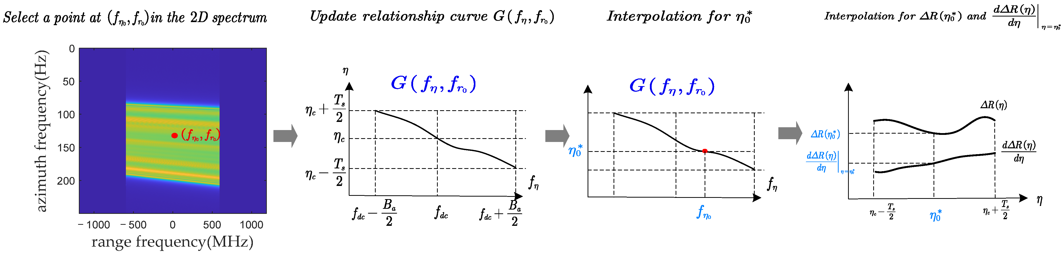
Select a point at the two-dimensional spectrum: We select a point on the two-dimensional spectrum, assuming it is located at the azimuth frequency $f_{{\eta }_0}$ and range frequency $f_{r_0}$.

(2)

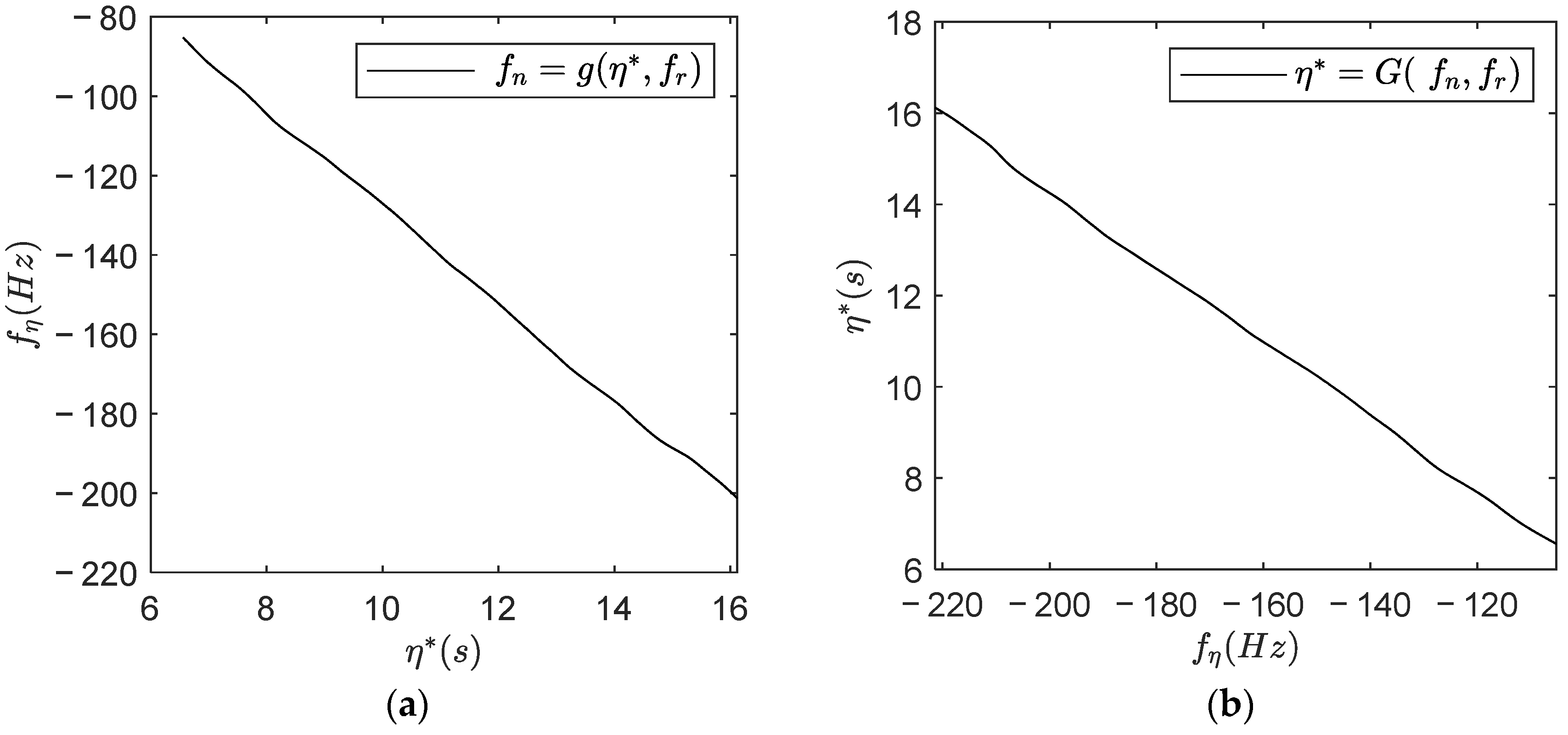
Update the relationship between ${\eta }^{*}$ and $f_{\eta }$ at $f_r$ = $f_{r_0}$: For range frequency $f_{r_0}$, a curve illustrating the relationship between ${\eta }^{*}$ and $f_{\eta }$ can be obtained based on Equation (6). This curve is similar to the one shown in Figure 2b, corresponding to the function ${\eta }^{*}$ = G($f_{\eta }$, $f_{r_0}$).

(3)

Interpolate the azimuth stationary phase time: For the point located at ($f_{{\eta }_0}$, $f_{r_0}$), ${\eta }_0^{*}$ is the azimuth stationary phase time corresponding to the azimuth frequency $f_{{\eta }_0}$. Based on the curve corresponding to the function ${\eta }^{*}$ = G($f_{\eta }$, $f_{r_0}$), we can obtain ${\eta }_0^{*}$ by interpolation.

(4)

Calculate the precise error in Equation (11): After obtaining the stationary phase time ${\eta }_0^{*}$, ${\left.{\displaystyle \frac{d\mathsf{\Delta }R\left(\eta \right)}{d\eta }}\right|}_{\eta ={\eta }_0^{*}}$ and $\mathsf{\Delta }R\left({\eta }_0^{*}\right)$ can be further obtained by interpolation. Then, $\mathsf{\Delta }{R}_{real}\left({\eta }_0^{*}\right)$ can be obtained.

(5)

Calculate the complete error in the two-dimensional frequency domain: Repeat Steps 1–4 to calculate the errors $\mathsf{\Delta }{R}_{real}\left({\eta }^{*}\right)$ at each frequency point in the two-dimensional frequency domain.

(6)

Perform Stolt interpolation on $\mathsf{\Delta }{R}_{real}\left({\eta }^{*}\right)$: The $\mathsf{\Delta }{R}_{real}\left({\eta }^{*}\right)$ is the actual error in the two-dimensional frequency domain before Stolt interpolation. To obtain the actual error after imaging, Stolt interpolation needs to be performed on $\mathsf{\Delta }{R}_{real}\left({\eta }^{*}\right)$.

Figure 3 describes the calculation process of steps 1 to 4.

2.4. An Improved PTA for Refocusing Building Surfaces

From the previous discussion, it is known that for multi-rotor UAV-borne SAR systems equipped with high-precision POSs, focusing on ground targets is generally straightforward. However, buildings that are significantly higher than the ground level are prone to defocusing and therefore require refocusing.

To refocus defocused buildings, this paper proposes an improved PTA based on the precise error model described above. The improved PTA compensates for exact errors in the two-dimensional frequency domain instead of approximate errors in the traditional range Doppler domain.

Considering the spatial variability of the errors, this improved PTA, like the traditional PTA, performs point-by-point compensation. The complete steps of MOCO + ω-k + the improved PTA are as follows:

(1)

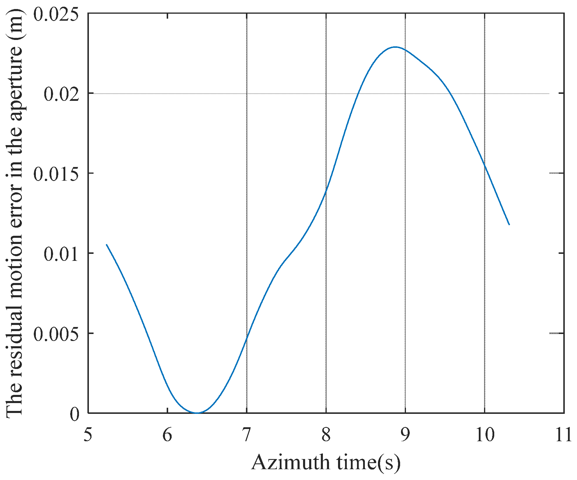
Motion compensation: OSA is performed on the RAW data to compensate for range-varying motion errors. After performing MOCO using the OSA, the residual error is generally small and therefore does not destroy the one-to-one relationship between ${\eta }^{*}$ and $f_{\eta }$.

(2)

Azimuthal resampling is performed to eliminate errors due to non-uniform sampling.

(3)

The ω-k algorithm is used for imaging to produce SAR images. At this stage, ground targets in the SAR images are well-focused, while building targets are severely defocused.

(4)

A pixel point is selected, N pixel points are taken along the range and azimuth directions centered on this pixel point to obtain the local SAR image. Based on practical experience, N is typically set to 64 or 128.

(5)

A two-dimensional fast Fourier transform (FFT) is performed on the selected local SAR image to obtain the signal in the two-dimensional frequency domain.

(6)

Based on the position of the pixels selected in Step 4 and combined with the elevation data, the exact error as described in Equation (11) is calculated according to the method proposed in this paper.

(7)

Phase compensation is performed in the two-dimensional frequency domain and the two-dimensional inverse fast Fourier transform (IFFT) is performed to obtain focused local SAR images. At this stage, the center of the local image is well-focused.

(8)

The pixel selected in Step 4 is replaced with the center pixel of the focused local image obtained in Step 7.

(9)

The next pixel is selected and the above process is repeated until all pixels are processed.

The complete flowchart of the improved PTA is shown in Figure 4.

3. Experimental Results and Analysis

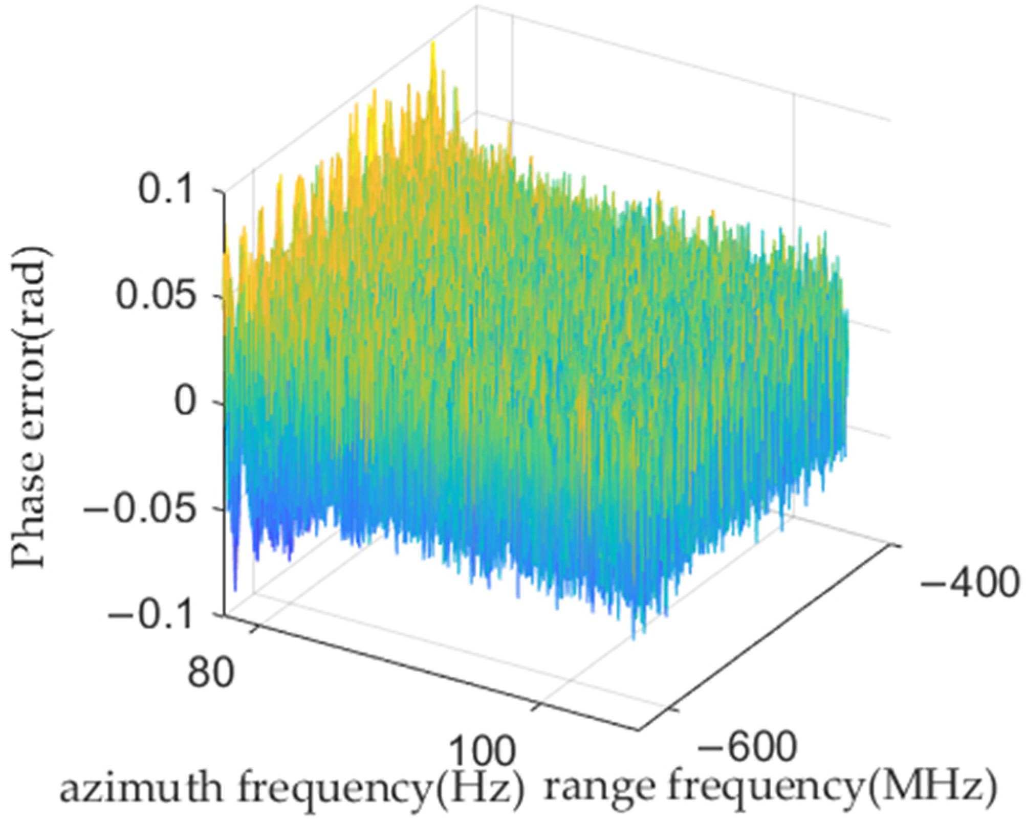
3.1. Calculation Accuracy Analysis

Previously, we introduced a method to calculate the accurate error in the two-dimensional frequency domain. To verify the accuracy and effectiveness of this method, this section will use actual multi-rotor UAV-borne SAR trajectories and system parameters to simulate the SAR data. The multi-rotor UAV-borne SAR system continuously transmits the FMCW signal and the main parameters in the simulation experiments are given in

Table 1. The main parameters in the simulation experiments.

Parameter	Symbol	Value
Carrier frequency	$f_c$	15.2 GHz
Bandwidth	$B_r$	1200 MHz
Reference range	$R_{ref}$	650 m
Pulse repetition frequency	$prf$	250 Hz
Azimuth beamwidth	$B_w$	3°
Speed of flight	$V$	8 m/s
Squint angle	$\theta$	−5.2°
Flight height	$H$	400 m

.

It can be seen from the parameters that the flight altitude of the multi-rotor UAV is only 400 m, which causes scene elevation to have a large impact on the residual error. We simulate a point target placed on the roof of the building with a height of 55 m. The residual motion error within the synthetic aperture is plotted in Figure 5.

The two-dimensional frequency domain signal is shown in Figure 6, and the range zero frequency is moved to the middle of the image. Due to the presence of a squint angle, the Doppler center frequency is not zero. The signal in the red rectangular region shown in Figure 6 is selected for analyzing the phase accuracy in Equations (8) and (9).

For each frequency point in the two-dimensional spectrum, the precise stationary phase time ${\eta }_0^{*}$ is calculated, subsequently allowing for the calculation of ${\left.{\displaystyle \frac{d\mathsf{\Delta }R\left(\eta \right)}{d\eta }}\right|}_{\eta ={\eta }_0^{*}}$ and $\mathsf{\Delta }R\left({\eta }_0^{*}\right)$. Then, the phase described in Equations (8) and (9) will be calculated.

The conjugate multiplication of the signals within the red rectangular region of Figure 6a and the signals described in Equations (8) and (9) is performed, and then, the phase of the signal after the conjugate multiplication is extracted. Figure 7a shows the phase after the conjugate multiplication with the signals described in Equation (8) and Figure 7b shows the phase after the conjugate multiplication with the signals described in Equation (9).

As can be seen in Figure 7, the approximated model in Equation (9) has a certain amount of phase error, whereas the exact model, represented by Equation (8), has almost no phase error.

According to Equations (10) and (12), the exact two-dimensional frequency domain phase error after Stolt interpolation can be calculated.

The conjugate multiplication of the signals within the red rectangular region in Figure 6b and the signals described in Equation (13) is performed, and then, the phase is extracted. The phase is shown in Figure 8. As can be seen in Figure 8, we can see that the exact model, represented by Equation (13), has almost no phase error.

From Figure 8, it can be seen that the errors calculated using the numerical computation method described in this paper closely match the errors in the simulated signal.

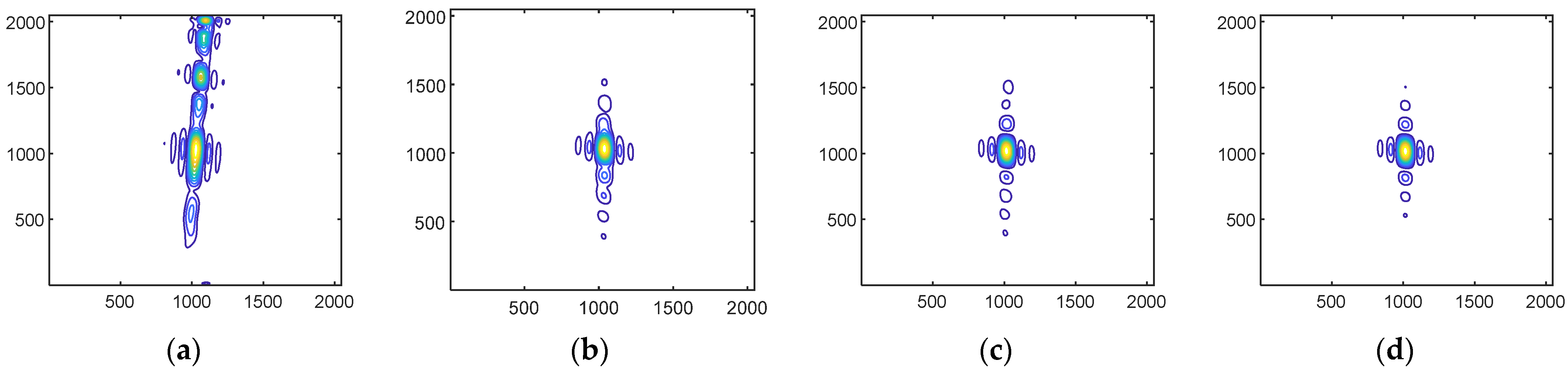
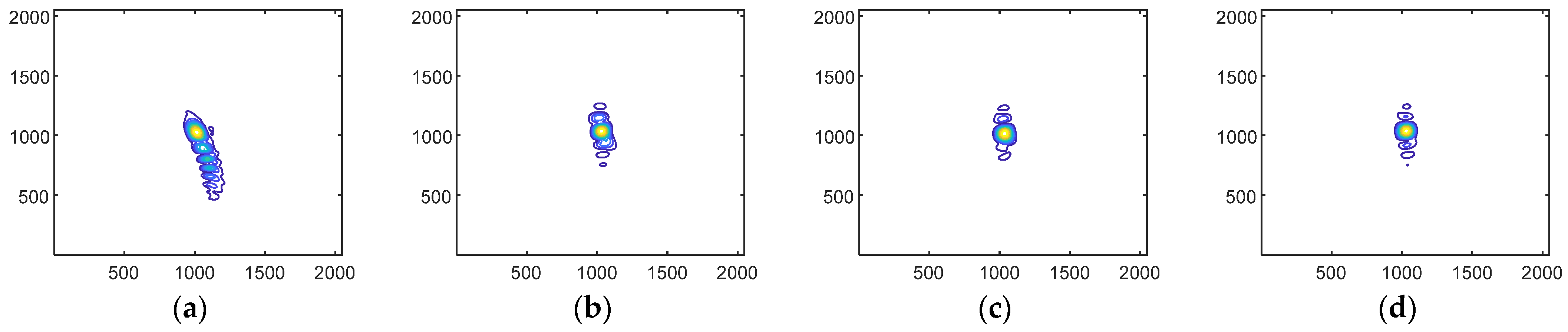
3.2. Simulation Experiments for Improved PTA

In this paper, we further propose a new and improved PTA. Next, we verify the effectiveness of this method through the simulation of point targets. Based on the parameters listed in Table 1, further simulation experiments are carried out by setting a point target on the roof of a building at 70 m. Subsequently, echo simulations are performed based on the position of this point and the actual flight trajectory; motion compensation is then performed based on ground elevation, followed by imaging processing using the ω-k algorithm. As shown in Figure 9a, there is a severe defocusing of the point target because the motion compensation is based on ground elevation, while the point target is located on a building surface at an elevation of 70 m. This leads to a significant discrepancy between the compensated errors and the actual errors. Since the elevation of this point is known, we can calculate the residual errors within the synthetic aperture based on this elevation. The challenge now is how to perform high-precision compensation on the image. We use the traditional improved PTA, the CMBP algorithm, and the improved PTA proposed in this paper to implement the compensation process and compare the accuracy of these compensations.

Figure 9b shows the effects of compensation using the traditional improved PTA, Figure 9c shows the effects of compensation using the CMBP algorithm, and Figure 9d shows the effects of compensation using the improved PTA proposed in this paper. It can be seen that the traditional improved PTA yields lower-quality results, while both the CMBP approach and the proposed improved PTA achieve a better focus.

The traditional improved PTA performs poorly because it only accounts for errors in the azimuth frequency domain and does not compensate for errors that vary within the range frequency. The CMBP method achieves better results; however, it uses approximations as shown in Equation (9) during its derivation, leading to images that are not of the best quality. The method proposed in this paper does not involve any approximations and, theoretically, can achieve complete compensation for the error phase.

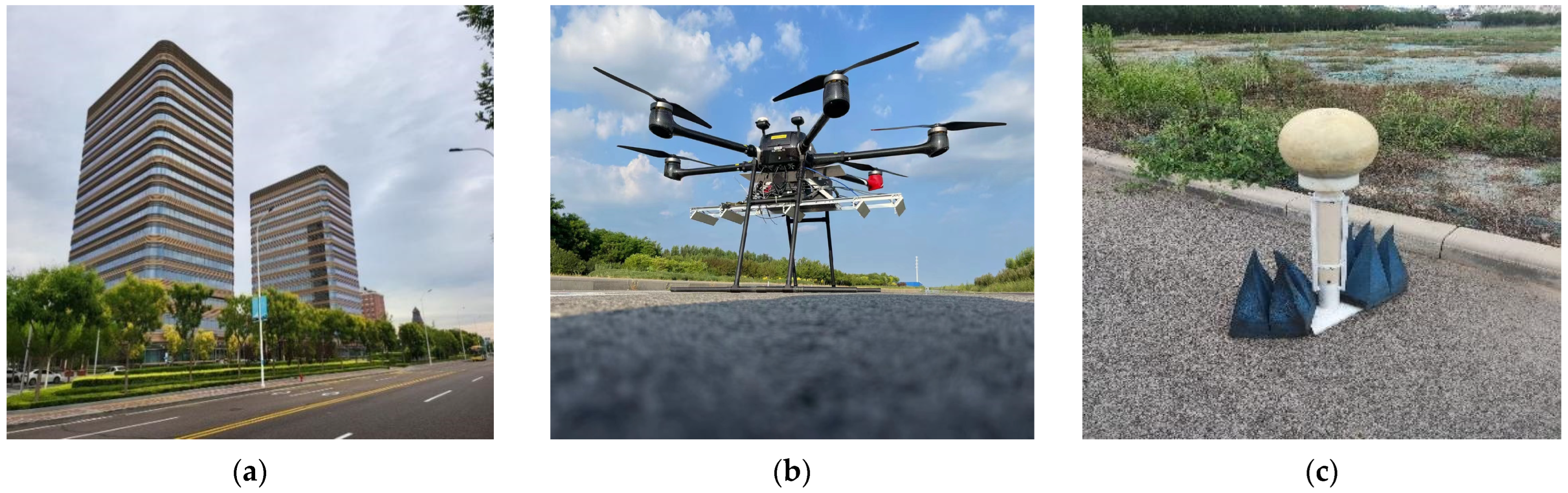
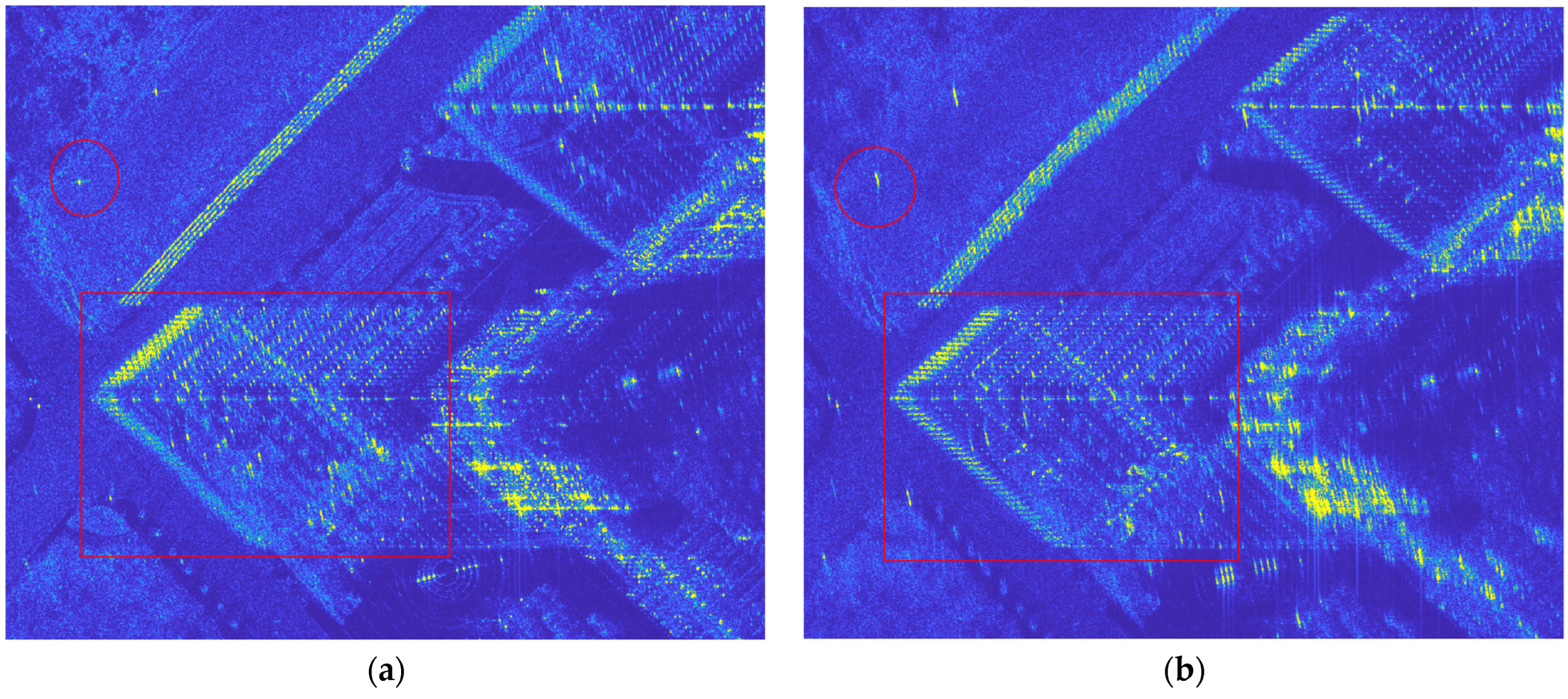
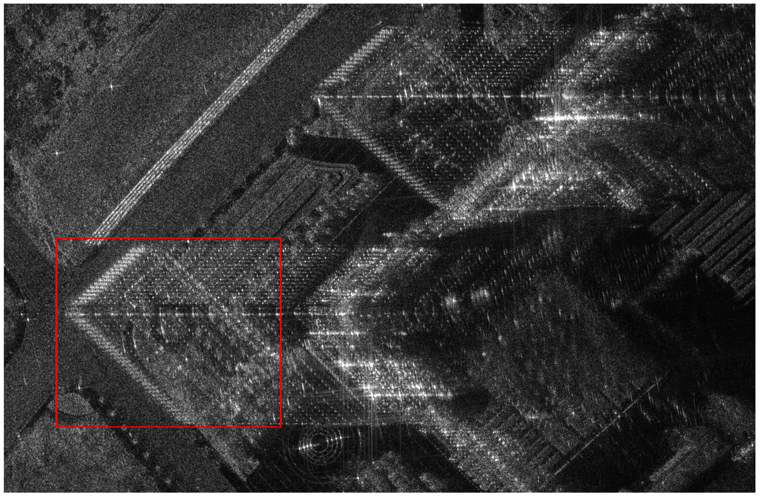
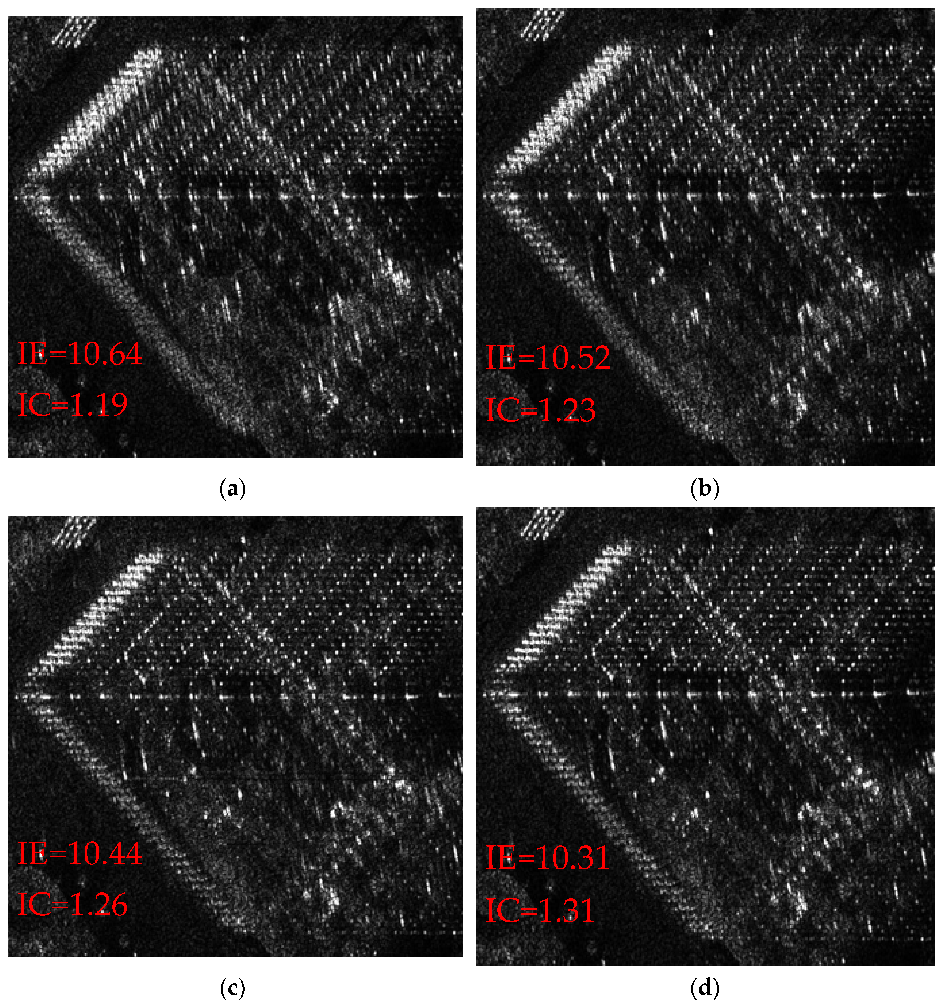
3.3. Actual SAR Data Results

To further verify the effectiveness of the proposed algorithm, the actual data of the multi-rotor UAV-borne-SAR system are used to compare the effectiveness of the proposed algorithm, the traditional improved PTA, and the CMBP algorithm.

Figure 10 displays the photos of the experimental scene and the experimental equipment. Figure 10a shows that the target area for this experiment is the Lin-gang business building, which is located in Tianjin, China. The photos of the multi-rotor UAV-borne-SAR system are shown in Figure 10b. To verify the effect of the proposed algorithm, we placed some Luneburg-lens reflectors on the ground. The elevation of the Luneburg-lens reflectors is about 2 m, and its photo is shown in Figure 10c.

Table 2. The main parameters in the actual experiments.

Parameter	Symbol	Value
Carrier frequency	$f_c$	15.2 GHz
Bandwidth	$B_r$	1200 MHz
Reference range	$R_{ref}$	650 m
Pulse repetition frequency	$prf$	250 Hz
Azimuth beamwidth	$B_w$	3°
Speed of flight	$V$	7.89 m/s
Squint angle	$\theta$	−7.86°
Flight height	$H$	402 m

shows the main parameters in this experiment. It can be seen that the UAV flies at an altitude of only 402 m and, due to factors such as the UAV’s weight and atmospheric turbulence, there is a −7.86° squint angle during data collection. This causes a significant discrepancy between the errors in building targets and ground targets. After performing motion compensation and imaging based on ground elevation, ground targets are well-focused while building surfaces are severely defocused.

To more clearly illustrate the impact of elevation on motion errors, we performed motion compensation and imaging processing at different elevations and compared the results.

Figure 11 shows the results of the imaging process by setting different reference elevations. Figure 11a shows the results after motion compensation and ω-k processing based on the 2 m reference elevation, with the Lin-gang business building in the red rectangle and the Luneburg-lens reflectors in the red ellipse. It can be seen that targets on the ground are well-focused, while the building is severely defocused. Figure 11b shows the results of motion compensation and imaging processing based on the 60 m reference elevation. Contrary to Figure 11a, the building in the image is well-focused, while the targets on the ground are severely defocused. It can be seen that for multi-rotor UAV-borne SAR, it is difficult to obtain a well-focused image of the whole scene based on a uniform elevation, and it is necessary to refocus the targets that are defocused due to elevation based on the SAR image.

To more intuitively demonstrate the processing effects of the proposed method and compare it with two other methods, we refocused the defocused Luneburg-lens shown in Figure 11b using the methods described above and compared the results of these methods.

Since the elevation of the Luneburg-lens reflector is about 2 m, we set the relative elevation to −58 m in the post-processing step and used the traditional improved PTA, the CMBP algorithm, and the algorithm proposed in this paper for processing. The processing results are shown in Figure 12.

Figure 13 shows the azimuthal pulse responses of the Luneburg-lens reflector processed using three methods.

Table 3. Focusing performance comparison.

Method	IRW(m)	PLSR (dB)	ILSR (dB)
Traditional improved PTA	0.303	−9.752	−7.416
CMBP algorithm	0.301	−11.524	−11.460
Proposed improved PTA	0.295	−13.515	−10.773

shows the azimuth 3-dB impulse response width (IRW), the peak-to-side lobe ratio (PSLR), and the integral sidelobe ratio (ISLR) of the azimuthal pulse responses.

According to Figure 12 and Figure 13, it can be seen that all of these methods can improve the focusing quality of the Luneburg-lens reflector. Among them, the result processed using the proposed method has the best focusing quality, while the result processed using the traditional improved PTA has the worst focusing quality. The result processed using the CMBP algorithm is essentially focused, but there still exists a slight sidelobe elevation and sidelobe asymmetry.

Next, on the SAR image based on the 2 m elevation processing shown in Figure 11a, we show how to refocus the building using the proposed method.

We first set the elevation value according to the location of the building in the defocused image; the set elevation of the building is shown in Figure 14a. The overlay results of the elevation image and the defocused building image are shown in Figure 14b. Finally, based on the elevation set in Figure 14a, the proposed method and traditional improved PTA are used to refocus the defocused building.

The SAR image of the building processed using the proposed method is shown in Figure 15. Figure 16 shows the results of using different algorithms for the target in the red rectangle in Figure 15. Figure 16a shows the localized image after performing one-step motion compensation and processing bythe ω-k algorithm, the results after post-processing using the traditional improved PTA are shown in Figure 16b, the results after post-processing using the CMBP algorithm are shown in Figure 16c, and the result after post-processing using the proposed method is shown in Figure 16d.

Figure 16 shows the processing results of several algorithms, with the image entropy (IE) of the results indicated. The image entropy and image contrast of the processing results are also listed in

Table 4. Focusing performance comparison.

Method	Image Entropy (IE)	Image Contrast (IC)
Result of ω-k	10.64	1.19
Result of ω-k +traditional improved PTA	10.52	1.23
Result of ω-k +CMBP	10.44	1.26
Result of ω-k +proposed improved PTA	10.31	1.31

. From the processing results, it can be observed that the algorithms used in the experiment can all improve the quality of the building targets in Figure 16a. Among these, the traditional improved PTA has the worst quality, while the method proposed in this paper achieves the best quality, with the lowest image entropy.

4. Discussion

The method proposed in this paper aims to address the significant defocusing of building targets in UAV-borne SAR images, which occurs due to their relatively high elevations. The method proposed in this paper primarily addresses how to achieve high-precision error compensation based on high-precision POSs, ensuring that the quality of the SAR image reaches theoretical values. Therefore, autofocus methods are not within the scope of this discussion.

In the scenarios discussed in this paper, the UAV’s low flight altitude and squint angles cause significant differences in motion errors among targets at different elevations. This makes it impossible to uniformly compensate for the errors of the entire scene. Consequently, ground targets will be focused but building targets remain defocused. Therefore, further error compensation is necessary for the defocused buildings.

Based on high-precision POS data and the known building elevation, we can calculate the residual error within the synthetic aperture for each pixel. However, these errors change after processing by the ω-k algorithm. Precisely calculating the errors after processing by the ω-k algorithm is the key to this study.

The traditional improved PTA and the CMBP algorithm have the same objective as the method proposed in this paper, but they involve different approximations in their derivation processes. The CMBP algorithm is derived based on Equation (9), which is the approximation of Equation (8). The traditional improved PTA does not account for errors in the range frequency domain at all, resulting in the poorest quality. The method proposed in this paper calculates errors based on the exact spectrum shown in Equation (8). Equation (8) does not use any approximations and is completely accurate. In Equation (8), we did not directly substitute Equation (6) into Equation (8). Therefore, both the azimuth time ${\eta }^{*}$ and the azimuth frequency $f_{\eta }$ are present in Equation (8). This is because Equation (6) is affected by errors and cannot be fully expressed as a function of $f_{\eta }$ without approximations. However, this does not affect our ability to calculate the precise spectrum. Due to the coupling between errors and the time–frequency relationship, it is impossible to obtain an analytical solution to Equation (8). Nevertheless, the exact solution to Equation (8) can be accurately computed using numerical methods. This process not only maintains high accuracy but also involves simple calculations. Figure 3 illustrates the process of solving Equation (8) using numerical methods. In the simulation experiments, we first analyze the error accuracy. Figure 7a shows the difference between the spectrum given by Equation (8) and the simulated point target spectrum; we can see that the difference between the two-dimensional spectrum phase of the simulated point target and the calculated two-dimensional spectrum phase is very small.

By comparing the phase of Equation (8) with the ideal two-dimensional frequency spectrum, we can obtain the accurate error in the two-dimensional frequency domain, as described by Equation (11). This error becomes more complex compared to the original time-domain error $\mathsf{\Delta }R\left(\eta \right)$. Performing Stolt interpolation on $\mathsf{\Delta }{R}_{real}\left({\eta }^{*}\right)$, the error $\mathsf{\Delta }{R}_{real}^{stolt}\left({\eta }^{*}\right)$ after ω-k processing can be obtained and the two-dimensional frequency spectrum is described in Equation (13). Figure 8 shows the difference between the spectrum given by Equation (13) and the simulated point target spectrum, and the difference between the simulated point target spectrum and the calculated spectrum is very small. The above simulation experiments verify the accuracy of the spectrum phase calculation method proposed in this paper.

Next, we combined the proposed spectrum calculation method with the traditional PTA to propose a new and improved PTA for refocusing defocused targets. Figure 4 illustrates the algorithm’s workflow. Then, we validated the improved PTA through simulations and real data experiments. Figure 9 shows the processing results based on the simulation data and compares them with two of the latest algorithms in this field. Subsequently, we further processed the actual data. First, motion compensation was performed based on an elevation of 60 m, while the Luneburg-lens placed on the ground had an elevation of 2 m. Clearly, the calculated motion error during motion compensation significantly differed from the actual error of the Luneburg-lens. This discrepancy results in substantial residual errors after motion compensation, leading to defocusing in the image. In contrast, the building targets, having an elevation consistent with the set elevation, are well-focused after imaging. We applied the aforementioned algorithms to refocus the defocused Luneburg-lens reflector and measured the azimuthal pulse response, PSLR, and ISLR after refocusing. This allows for a quantitative comparison of the processing effects. Finally, we demonstrated how the proposed method can be used to refocus the defocused building facade in Figure 11a. We also compared the processing effects of several algorithms and the image entropy of the final results.

5. Conclusions

During the motion compensation process for multi-rotor UAV-borne SAR systems, buildings may be defocused due to mismatches between the actual elevation and the reference elevation. To address this issue, this paper proposed a novel improved PTA that avoids any approximation calculations while remaining computationally simple. To validate the effectiveness of the proposed method, both simulation and actual data processing experiments were conducted. First, the computational accuracy of the proposed method was analyzed through simulations. The simulation experiments demonstrated that the difference between the two-dimensional frequency domain phase calculated using the proposed method and the simulated point target frequency domain phase was less than 0.15 rad. Subsequently, further comparative experiments using both simulated and actual data were conducted. The refocusing of simulated point targets and an actual Luneburg-lens reflector was performed to compare the processing effects of several of the latest algorithms in this field. The PSLR and ISLR after processing were listed. The results from both simulation and actual data experiments showed that the proposed method was better than the other two methods. Finally, the process of refocusing a defocused building using the proposed method was demonstrated, achieving the successful refocusing of the building.

References

- Curlander, J.; McDonough, R. Synthetic Aperture Radar: Systems and Signal Processing; Wiley: New York, NY, USA, 1991. [Google Scholar]
- Chen, J.; Xing, M.; Yu, H.; Liang, B.; Peng, J.; Sun, G.-C. Motion Compensation/Autofocus in Airborne Synthetic Aperture Radar: A Review. IEEE Geosci. Remote Sens. Mag. 2022, 10, 185–206. [Google Scholar] [CrossRef]
- Mao, X.; He, X.; Li, D. Knowledge-Aided 2-D Autofocus for Spotlight SAR Range Migration Algorithm Imagery. IEEE Trans. Geosci. Remote Sensing. 2018, 56, 5458–5470. [Google Scholar] [CrossRef]
- Xu, W.; Wang, B.; Xiang, M.; Song, C.; Wang, Z. A Novel Autofocus Framework for UAV SAR Imagery: Motion Error Extraction from Symmetric Triangular FMCW Differential Signal. IEEE Trans. Geosci. Remote Sens. 2022, 60, 1–15. [Google Scholar] [CrossRef]
- Xu, W.; Wang, B.; Xiang, M.; Li, R.; Li, W. Image Defocus in an Airborne UWB VHR Microwave Photonic SAR: Analysis and Compensation. IEEE Trans. Geosci. Remote Sens. 2022, 60, 1–18. [Google Scholar] [CrossRef]
- Zhang, L.; Sheng, J.; Xing, M.; Qiao, Z.; Xiong, T. Wavenumber-Domain Autofocusing for Highly Squinted UAV SAR Imagery. IEEE Sens. J. 2012, 12, 1574–1588. [Google Scholar] [CrossRef]
- Brancato, V.; Jäger, M.; Scheiber, R.; Hajnsek, I. A Motion Compensation Strategy for Airborne Repeat-Pass SAR Data. IEEE Geosci. Remote Sens. Lett. 2018, 15, 1580–1584. [Google Scholar] [CrossRef]
- Meng, D.; Hu, D.; Ding, C. A New Approach to Airborne High-Resolution SAR Motion Compensation for Large Trajectory Deviations. Chin. J. Electron. 2012, 21, 764–769. [Google Scholar]
- Yang, M.; Zhu, D. Efficient Space-Variant Motion Compensation Approach for Ultra-High-Resolution SAR Based on Subswath Processing. IEEE J. Sel. Top. Appl. Earth Obs. Remote Sens. 2018, 11, 2090–2103. [Google Scholar] [CrossRef]
- Fornaro, G.; Franceschetti, G.; Perna, S. Motion compensation errors: Effects on the accuracy of airborne SAR images. IEEE Trans. Aerosp. Electron. Syst. 2005, 41, 1338–1352. [Google Scholar] [CrossRef]
- Huai, Y.; Liang, Y.; Ding, J.; Xing, M.; Zeng, L.; Li, Z. An Inverse Extended Omega-K Algorithm for SAR Raw Data Simulation With Trajectory Deviations. IEEE Geosci. Remote Sens. Lett. 2016, 13, 826–830. [Google Scholar] [CrossRef]
- Zheng, X.; Yu, W.; Li, Z. A Novel Algorithm for Wide Beam SAR Motion Compensation Based on Frequency Division. In Proceedings of the 2006 IEEE International Symposium on Geoscience and Remote Sensing, Denver, CO, USA, 31 July–4 August 2006; IEEE: Piscataway, NJ, USA, 2006; pp. 3160–3163. [Google Scholar]
- Prats, P.; Camara De Macedo, K.A.; Reigber, A.; Scheiber, R.; Mallorqui, J.J. Comparison of Topography- and Aperture-Dependent Motion Compensation Algorithms for Airborne SAR. IEEE Geosci. Remote Sens. Lett. 2007, 4, 349–353. [Google Scholar] [CrossRef]
- Prats, P.; Reigber, A.; Mallorqui, J.J. Topography-Dependent Motion Compensation for Repeat-Pass Interferometric SAR Systems. IEEE Geosci. Remote Sens. Lett. 2005, 2, 206–210. [Google Scholar] [CrossRef]
- de Macedo, K.A.; Scheiber, R. Precise Topography- and Aperture-Dependent Motion Compensation for Airborne SAR. IEEE Geosci. Remote Sens. Lett. 2005, 2, 172–176. [Google Scholar] [CrossRef]
- Wang, G.; Zhang, L.; Li, J.; Hu, Q. Precise Aperture-dependent Motion Compensation for High-resolution Synthetic Aperture Radar Imaging. IET Radar Sonar Navig. 2017, 11, 204–211. [Google Scholar] [CrossRef]
- Perna, S.; Zamparelli, V.; Pauciullo, A.; Fornaro, G. Azimuth-to-Frequency Mapping in Airborne SAR Data Corrupted by Uncompensated Motion Errors. IEEE Geosci. Remote Sens. Lett. 2013, 10, 1493–1497. [Google Scholar] [CrossRef]
- Lu, Q.; Du, K.; Li, Q. Improved Precise Tomography- and Aperture-Dependent Compensation for Synthetic Aperture Radar. In Proceedings of the 2021 2nd China International SAR Symposium (CISS), Shanghai, China, 3–5 November 2021. [Google Scholar]
- Meng, D.; Hu, D.; Ding, C. Precise Focusing of Airborne SAR Data With Wide Apertures Large Trajectory Deviations: A Chirp Modulated Back-Projection Approach. IEEE Trans. Geosci. Remote Sens. 2015, 53, 2510–2519. [Google Scholar] [CrossRef]
- Meng, D.; Ding, C.; Hu, D.; Qiu, X.; Huang, L.; Han, B.; Liu, J.; Xu, N. On the Processing of Very High Resolution Spaceborne SAR Data: A Chirp-Modulated Back Projection Approach. IEEE Trans. Geosci. Remote Sens. 2018, 56, 191–201. [Google Scholar] [CrossRef]
- Zhang, L.; Li, H.; Qiao, Z.; Xu, Z. A Fast BP Algorithm With Wavenumber Spectrum Fusion for High-Resolution Spotlight SAR Imaging. IEEE Geosci. Remote Sens. Lett. 2014, 11, 1460–1464. [Google Scholar] [CrossRef]
- Li, Y.; Liang, X.; Ding, C.; Zhou, L.; Ding, Q. Improvements to the Frequency Division-Based Subaperture Algorithm for Motion Compensation in Wide-Beam SAR. IEEE Geosci. Remote Sens. Lett. 2013, 10, 1219–1223. [Google Scholar]
- Chen, M.; Qiu, X.; Li, R.; Li, W.; Fu, K. Analysis and Compensation for Systematical Errors in Airborne Microwave Photonic SAR Imaging by 2-D Autofocus. IEEE J. Sel. Top. Appl. Earth Obs. Remote Sens. 2023, 16, 2221–2236. [Google Scholar] [CrossRef]