Article

Radar Emitter Recognition Based on Spiking Neural Networks

College of Electronic Science and Technology, National University of Defense Technology, Changsha 410073, China
*
Author to whom correspondence should be addressed.
Remote Sens. 2024, 16(14), 2680; https://doi.org/10.3390/rs16142680 (registering DOI)
Submission received: 2 June 2024 / Revised: 13 July 2024 / Accepted: 17 July 2024 / Published: 22 July 2024
(This article belongs to the Special Issue Technical Developments in Radar—Processing and Application)

Abstract

:
Efficient and effective radar emitter recognition is critical for electronic support measurement (ESM) systems. However, in complex electromagnetic environments, intercepted pulse trains generally contain substantial data noise, including spurious and missing pulses. Currently, radar emitter recognition methods utilizing traditional artificial neural networks (ANNs) like CNNs and RNNs are susceptible to data noise and require intensive computations, posing challenges to meeting the performance demands of modern ESM systems. Spiking neural networks (SNNs) exhibit stronger representational capabilities compared to traditional ANNs due to the temporal dynamics of spiking neurons and richer information encoded in precise spike timing. Furthermore, SNNs achieve higher computational efficiency by performing event-driven sparse addition calculations. In this paper, a lightweight spiking neural network is proposed by combining direct coding, leaky integrate-and-fire (LIF) neurons, and surrogate gradients to recognize radar emitters. Additionally, an improved SNN for radar emitter recognition is proposed, leveraging the local timing structure of pulses to enhance adaptability to data noise. Simulation results demonstrate the superior performance of the proposed method over existing methods.

1. Introduction

Radar emitter recognition is a critical component of electromagnetic environment awareness. Efficient and effective recognition of radar emitters is essential for subsequent tasks such as platform recognition, target tracking, and related actions [1]. However, the electromagnetic environment has grown increasingly complex with advancements in electronic systems like radar, navigation, and communication, rendering traditional methods ineffective for radar emitter recognition tasks.
Data used for radar emitter recognition can be categorized primarily into two types. The first type is pulse description words (PDWs), which encompass parameters such as time of arrival (TOA), pulse width (PW), radio frequency (RF), and direction of arrival (DOA). By calculating the first-order differential time of arrival (DTOA), the pulse repetition interval (PRI) of a radar can be obtained, reflecting the timing pattern followed by the radar when emitting pulses [2]. PDWs are widely used due to their ease of acquisition across various application scenarios. The second type is intra-pulse features, which are utilized for specific emitter identification [3] or intra-pulse modulation type identification [4]. However, intra-pulse features require significant storage, transmission, and processing resources, making them impractical in drone-borne and airborne electronic reconnaissance scenarios.
Traditional methods for radar emitter recognition typically involve analyzing PDWs using statistical methods and obtaining typical parameters such as the PRI, PW, and RF of the target radar. Subsequently, feature parameter matching [5] or machine learning [6] is applied for recognition. The feature parameter matching method compares the statistical parameters of radar pulse trains with those stored in a database to obtain the corresponding radar type. Gong et al. proposed a radar emitter recognition method based on a pulse-matching template sequence and accelerated it with a parallel structure [7]. This method has the advantages of simple execution and fast recognition. A naive Bayesian classifier is used to recognize radar signals whose parameters obey normal distribution [8]. In [9], a normal distribution scale mixture model is established, which uses Bayesian treatment for model learning, supervised classification, and clustering to realize the effective treatment of missing values and outliers. A complex radar signal classification method based on weight-xgboost is proposed in [10]. This method uses different types of large datasets to train the model and solves the problem of data deviation by introducing a smooth weight function. In [11], a multilayer perceptron is used to recognize the intercepted radar data in the form of interval values. However, these methods often require manual feature design tailored to radar signal characteristics and struggle with high-dimensional features such as inter-pulse timing patterns, limiting their adaptability to scenarios with rapid parameter agility and significant data noise.
In recent years, deep learning techniques such as CNNs and RNNs have been applied to radar emitter recognition [12,13]. These methods achieve radar emitter recognition under extreme conditions by extracting and utilizing high-dimensional timing features. For example, in [14], Wang et al. transform radar pulse trains into two-dimensional feature maps and employed CNNs for recognition, effectively utilizing correlations between different radar pulse train parameters. In [15], Liu et al. first introduce RNNs to extract long-term timing patterns of radar pulse streams and further solve problems of classification, denoising, and deinterleaving of radar pulse streams. On this basis, Notaro et al. optimize the normalization method and the feature concatenating method and realize the recognition of 17 radar emitters using LSTM [16]. Li et al. further incorporate attention mechanisms to suppress data noise effectively [17]. In [18], a sequence-to-sequence LSTM network for a multifunction radar (MFR) work mode recognition is proposed, capable of recognizing various work modes and their transitions. In [19], Zhang et al. propose a multioutput multistructure learning-based framework based on an LSTM transformer to recognize fine-grained work modes of cognitive radar. Although the above methods based on deep learning have greatly improved the ability to process complex forms of signals and adapt to data noise, there are still two shortcomings. First, these methods are still susceptible to data noise because the existing methods use DTOA as the time dimension of the radar pulse train. When the data noise is serious, timing patterns in the DTOA sequence are seriously damaged, resulting in the timing patterns learned by these methods no longer matching the current situation [15]. Secondly, existing deep learning-based methods have high computational complexity. This is because these methods introduce complex gating mechanisms to improve the memory capacity of neural networks and require intensive floating-point numerical multiplication operations, which also results in a large amount of energy consumption [20,21].
To address the limitations of traditional deep learning methods in radar emitter recognition, spiking neural networks (SNNs) were introduced [22,23,24,25]. Figure 1 shows the differences between traditional artificial neural networks (ANNs) and SNNs in neuron models and information transmission. SNNs offer two primary advantages over ANNs. Firstly, SNNs are particularly suitable for processing time series data such as radar pulse trains due to the temporal dynamics and asynchronous spike-based information processing of spiking neurons. The above characteristics of spiking neurons make their data processing form more consistent with the radar pulse train, while the traditional neurons can only process information statically [22,25]. Secondly, SNNs perform accumulation calculations in an event-driven manner, where only neurons receiving spikes execute computations. In contrast, traditional ANNs require all neurons to perform floating-point multiplication operations for each input, leading to higher computational demands. These differences give SNNs a stronger processing ability for time series data and lower computational complexity. Furthermore, SNNs have demonstrated superior performance and higher computational efficiency in tasks such as speech recognition and neuromorphic data processing [24,25].
In this paper, a radar emitter recognition method based on SNNs is proposed. Initially, a neural coding method for radar pulses based on direct coding is introduced to encode radar pulse trains into spike trains. Subsequently, an SNN for radar emitter recognition is developed by integrating the leaky integrate-and-fire (LIF) neuron model and surrogate gradient training strategy to process the encoded spike trains. Finally, the class of the radar pulse train is then determined through rate decoding of spike trains in the output layer. Based on the above method, an improved SNN with stronger adaptability to data noise is proposed by improving the above coding method.
It should be noted that the proposed SNNs are different from existing SNNs. While existing SNNs have been successful in various research domains, they are not directly applicable to processing radar pulse trains. This is because most existing SNNs are mainly used for image processing rather than discrete radar pulses [23,24]. For example, for static images, existing methods first use rate coding to encode a single pixel value into a spike train randomly distributed over a fixed time length and then use fully connected SNNs for processing. In other fields, such as speech recognition [25] or radar emitter recognition [26], most of the existing methods first convert speech signals or radar pulse signals (intra-pulse features) into two-dimensional static images and then use the above image processing method to recognize them. However, the above spike coding and processing methods are inefficient and cannot fully utilize the sequential processing ability of SNNs. Therefore, we propose direct coding and local timing structure coding methods suitable for radar pulse train processing by using latent timing characteristics. In the direct coding method, radar pulses are first converted into embedding vectors using an embedding layer, which is then encoded into spike trains in the encoding layer. This method offers shorter coding times and reduces information loss compared to the rate coding methods commonly used in existing SNNs. Moreover, the local timing structure coding method enhances the utilization of timing characteristics within radar pulse trains, thereby mitigating the impact of data noise more effectively.
The contributions of this paper are listed as follows:
(1)
A radar emitter recognition framework based on SNNs with higher computational efficiency is proposed. Theoretical analysis and simulation experiments show that the proposed framework has lower computational complexity and energy consumption than traditional methods.
(2)
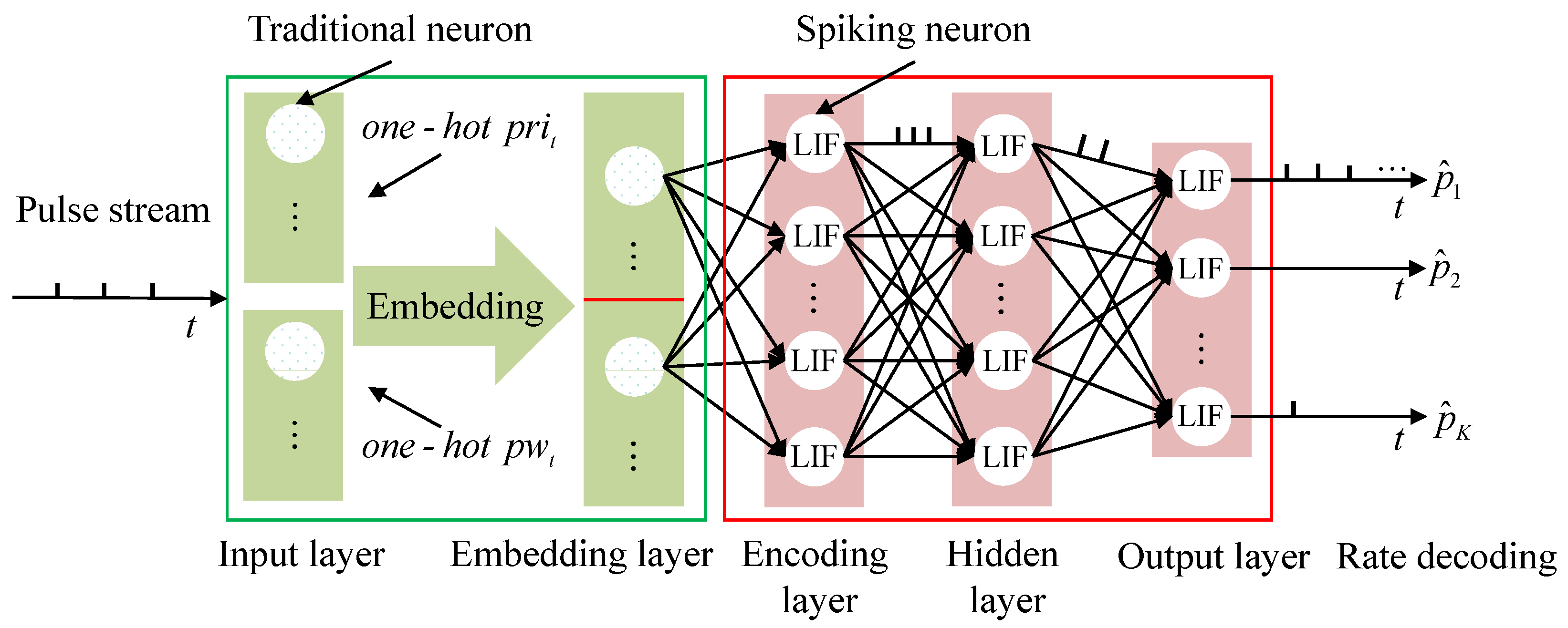
A direct coding method of radar pulse timing features is proposed to apply SNNs with stronger time series data processing ability to radar emitter recognition. Different from existing fixed coding methods, the proposed coding method can adaptively adjust the weight, thereby reducing the information loss in the coding process. Simulation results show that the proposed method has stronger data noise adaptability than the method based on traditional ANNs under the same input data form. This also proves that SNNs are more suitable for radar pulse train recognition than traditional ANNs.
(3)
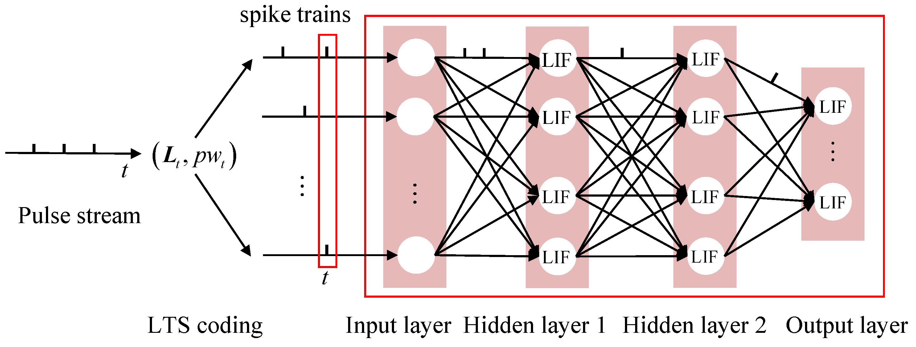
A radar pulse timing feature coding method based on local timing structure is proposed, which significantly enhances the data noise adaptability of the proposed method. By analyzing the essence of data noise splitting PRI features, the local DTOA sequence of radar pulses is proposed as PRI features of radar pulses, and the SNN is further improved. Experimental results show that the proposed radar emitter recognition method based on improved SNNs has much higher adaptability to data noise than other methods.
The rest of this article is organized as follows. Section 2 introduces the problems to be solved and related principles of SNNs. Section 3 presents the radar emitter recognition method based on SNNs. Section 4 evaluates the performance of the proposed method. Section 5 discusses the computational efficiency of the proposed method and its applicability to more complex radar signals. Finally, Section 6 provides the concluding remarks of the whole work.

2. Research Background

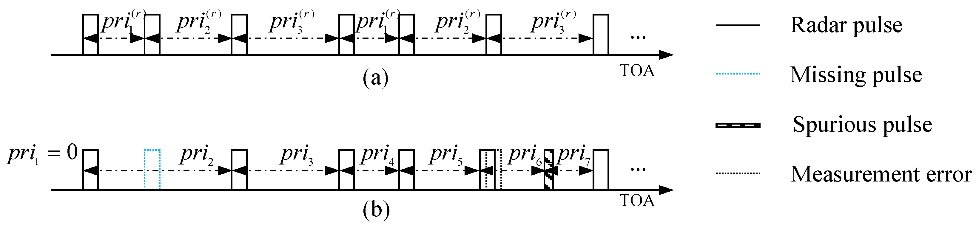
2.1. Problem Formulation

Statistical parameters of a radar pulse train are represented by PDWs. In a PDW, the PW, RF, DOA, and other parameters describe the statistical characteristics of a single pulse and are generally fixed, while the PA is not stable enough. After preprocessing intercepted pulses with the above statistical parameters, the TOA can be used as the main parameter for radar emitter recognition. This is because the TOA is easy to measure, and there is a high dimensional timing pattern in a TOA sequence, which can be described by the PRI pattern. For conventional radar, the PRI pattern is the basic time structure of periodic repetition in a pulse train. For example, the PRI pattern of the pulse train in Figure 2a can be represented as [ p r i 1 ( r ) , p r i 2 ( r ) , p r i 3 ( r ) ] . Different types of radars generally have different PRI patterns, so PRI patterns can be used as the main feature to recognize radar emitters [17]. Thus, this paper employs the PRI as the primary feature for radar emitter recognition while also considering PW to illustrate the combined use of the PRI with other parameters.
The TOA sequence of a pulse train transmitted by the radar can be expressed as
t = i = 1 N δ t t i
where t i denotes the arrival time of the ith pulse, δ ( · ) denotes the Dirac function, and N denotes the number of pulses in the pulse train.
The intercepted radar pulse train often includes significant data noise, categorized into three types: spurious pulses, missing pulses, and measurement errors. Spurious pulses primarily result from thermal noise in the receiver and pulses emitted by other radars. Missing pulses occur due to antenna scanning, signal propagation, and noise coverage. When the effect of radar signal sorting is poor, it will also lead to a large number of missing pulses and spurious pulses. In addition, due to the performance limitations of the receiver, there are also some measurement errors in parameters. Therefore, the TOA sequence of the intercepted radar pulse train can be expressed as
t = i = 1 N δ t t i ε i ( 1 m i ) + i = 1 N s δ t t i s
where ε i denotes the TOA measurement error of the ith pulse obeying the Gaussian distribution and m ( i ) is the indicator function of the missing pulse—when the ith pulse is missed, its value is 1, otherwise it is 0, and it obeys the Bernoulli distribution with probability ρ m in our simulations. t i ( s ) denotes the arrival time of the ith spurious pulse, and N s denotes the number of spurious pulses; in addition, the number of spurious pulses added between two adjacent pulses obeys the Poisson distribution with the mean of ρ s ( 1 ρ m ) in our simulations. ρ m and ρ s represent missing pulse rate and spurious pulse rate, respectively.
The three types of data noise are illustrated in Figure 2b. In the figure, the blue dotted rectangle represents missing pulses, the narrow rectangle filled with slashes represents spurious pulses, and the time offset between the black dotted rectangle and its left rectangle indicates measurement error. In comparison with Figure 2a, the presence of data noise severely disrupts the timing pattern of the pulse stream in Figure 2b. For instance, the missing pulse in the figure changes the time interval between the original first and second pulses to p r i 1 ( r ) + p r i 2 ( r ) , while the spurious pulse and measurement error split the interval p r i 3 ( r ) between the last two pulses into two segments.
The problem is to effectively utilize high-dimensional timing features from a pulse stream to recognize radar emitters despite data noise. By combining auxiliary parameters such as PW, the radar pulse train can be re-expressed as P = [ p r i 1 , p w 1 , p r i 2 , p w 2 , , p r i N , p w N ] , where p r i i = t i t i 1 , and t i denotes the ith pulse of the noise-contaminated TOA sequence in Equation (2). Each pulse train belongs to a specific radar type, and its category label can be represented by c 1 , K , where K denotes the total number of classes. Thus, the objective of our work can be formulated as follows:
f = arg min f E ( f ( P ) , c )
where E ( · ) represents the error function, f ( · ) is the pulse stream recognition function, f is the goal recognition function, and c is the real label of the radar pulse train. Therefore, the objective is to obtain the optimal model that minimizes the recognition error for radar pulse trains.
Existing deep learning-based methods, such as RNNs, have two main problems in the process of learning and using the above recognition function f ( · ) . Firstly, they require extensive computational resources during both the training and deployment phases. Secondly, they struggle to handle the PRI feature damage problem caused by data noise effectively. Therefore, we propose a radar emitter recognition method based on SNNs to solve the above problems, and related principles of SNNs are introduced in Section 2.2.

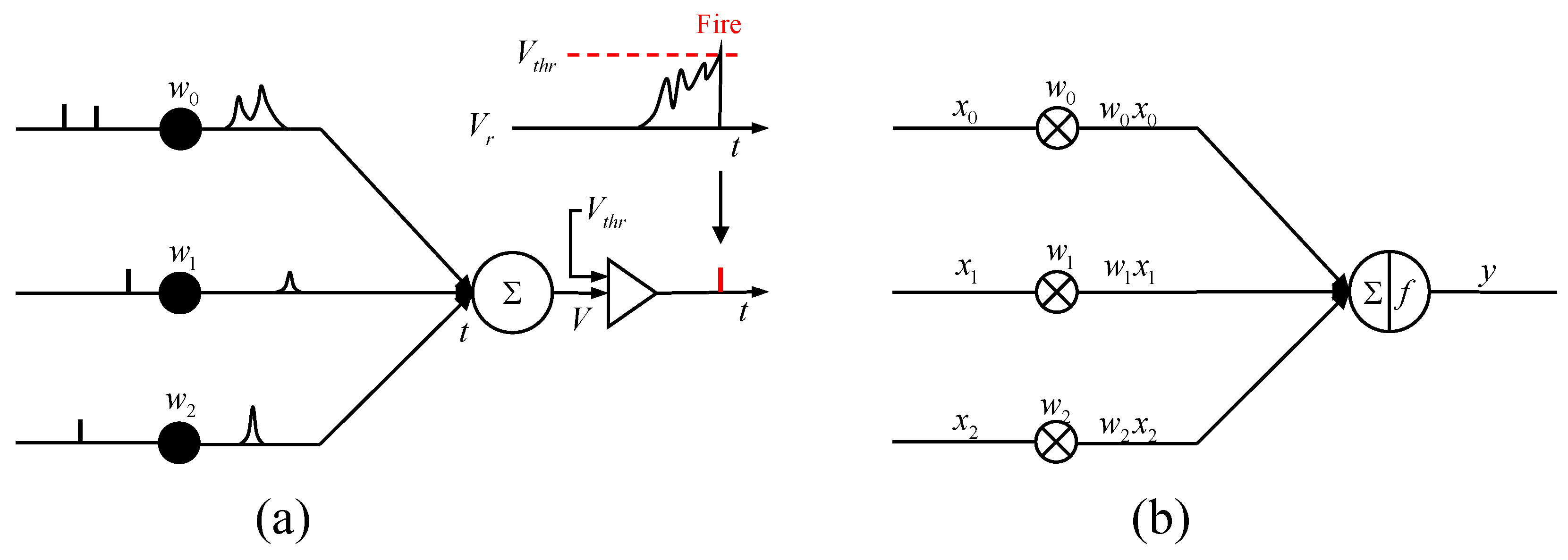
2.2. Spiking Neural Networks

By introducing temporal dynamics and a spiking mechanism into neuron models, SNNs can achieve stronger representation ability and higher computational efficiency, like biological neural networks [27]. In SNNs, information is transmitted in discrete and asynchronous spikes, enabling them to process spatio-temporal information more effectively. First of all, SNNs can effectively utilize the timing information between multiple spikes so that the processing of time series data can be realized more naturally. Secondly, the asynchronous spike-triggering mechanism ensures neurons perform accumulation operations only upon spike inputs, enhancing computational efficiency and reducing energy consumption.
Spiking neurons are the basic unit of SNNs. Many spiking neuron models have been proposed to describe the temporal dynamics of biological neurons, such as the Hodgkin–Huxley, Izhikevich, and leaky integrate-and-fire (LIF) neuron models. Among these neuron models, the LIF neuron model has lower computational complexity and is widely used in various methods [28]. Therefore, the LIF neuron is used as the basic neuron in this paper. The differential form of voltage dynamics of the LIF neuron is
τ m d V d t = V V r + R m I
where V represents the voltage of the neuron, V r represents the reset voltage, R m represents the membrane resistance, I represents the external input current, and τ m represents the membrane voltage time constant. The information processing mechanism of LIF neurons is shown in Figure 1a. In the figure, the black vertical line represents the time series input to the spiking neurons, also known as spikes, and the black solid circle represents the synapse. Each spike causes postsynaptic voltage after passing through the synapse, and the voltage increment of the neuron is equal to the accumulation of all postsynaptic voltages. When the voltage of the neuron exceeds the threshold V t h r , the neuron emits a spike and resets the voltage to V r . In order to facilitate calculation, we set V r = 0 mV.
The above equation is a continuous form, which is difficult to implement with the current deep learning framework. Therefore, we convert it into a form of voltage iterative update [29]
V t = 1 d t τ m V t 1 + d t τ m I
where t is the current time and d t is the time step. In the above equation, 1 d t τ m and d t τ m are constants. To facilitate representation, 1 d t τ m is redefined as τ . In the case where the LIF neuron is connected to multiple other neurons, I is the weight sum of other neurons’ output. Furthermore, by further taking into account the reset rule when the voltage of the spiking neuron exceeds the threshold, Equation (5) can be re-expressed as
V t = τ V t 1 1 s t + i w i s i t
s i t = g V i t V t h r
where w i represents the strength of the ith connection of the neuron, s t represents spikes fired by the current spiking neuron at time t, s i t represents spikes fired by the ith input neuron at time t, and g represents the step function. When the voltage exceeds the threshold V t h r , the value of s i t is 1, otherwise it is 0. From the above equation and Figure 1a, it can be seen that the spiking neuron will perform the accumulate operations when a spike arrives and the multiplication operation with higher complexity can be avoided, thus achieving higher computational efficiency. Moreover, the voltage of each neuron is related to its voltage at the previous moment. This self-recursive characteristic gives the spiking neuron the ability to process time series data that traditional neurons do not have.

3. Methodology

In this section, a radar emitter recognition method based on SNNs is proposed. In Section 3.1, a direct spike coding method of radar pulses is proposed to transform each radar pulse into spikes that can be processed by SNNs. Then, the specific structure and implementation details of the network are introduced in Section 3.2. In Section 3.3, the radar emitter recognition and network optimization strategy are introduced. Figure 3 shows the network structure used for radar emitter type recognition. The scatter-filled white circle in the figure represents non-spiking neurons (e.g., traditional neurons in ANNs), which corresponds to the floating-point number vector input into the SNNs. The neurons in the hidden layer and the output layer are spiking neurons. All the spiking neurons used are LIF neurons, and the output of the spiking neuron is a spike train in the form of a discrete time series. On the basis of Section 3.1, Section 3.2 and Section 3.3, an improved spiking neural network based on local timing structure coding is proposed in Section 3.4.

3.1. Timing Feature Coding of Radar Pulses

The radar pulse train needs to be encoded as spike trains to be processed by SNNs. In order to represent the data regularly and facilitate the processing of the machine, the continuous PRI and PW values are first digitized and converted into one-hot vectors. For the tth pulse’s parameters p r i t and p w t , the digitized results can be expressed as p r i t digit = p r i t / d p r i and p w t digit = p w t / d p w , respectively, where · represents the downward rounding operation, d p r i represents the quantization unit of PRI, and d p w represents the quantization unit of PW. Then, the digitized PRI and PW are converted into one-hot vectors. The maximum range of PRI is set to D p r i , and the maximum range of PW is set to D p w . When the PRI and PW values exceed this range, the digital PRI and PW are set to 0. The converted digital PRI can be expressed as g t p r i = 0 , , 1 , , 0 R L 1 × 1 with only its p r i t digit th value being 1, where L 1 = D p r i / d p r i + 1 . The converted digital PW can be expressed as g t p w R L 2 × 1 which is defined similar to g t p r i , where L 2 = D p w / d p w + 1 . In order to compress one-hot features and improve the stability of network learning, word embedding is used to transform g t p r i and g t p w into vectors with lower dimensions:
e t p r i = E p r i g t p r i
e t p w = E p w g t p w
where e p r i R l 1 × 1 and e p r i R l 2 × 1 are the embedded digital PRI and PW, respectively, and E p r i R l 1 × L 1 and E p w R l 2 × L 2 are the embedding matrices of PRI and PW, respectively, where l 1 L 1 and l 2 L 2 . The embedding matrix is randomly initialized and optimized during training.
Then, the embedded vectors are concatenated as the input of the encoding layer. The concatenated vector can be expressed as
x t = e t p r i ; e t p w
Finally, the concatenated vector x t is input into the encoding layer of the SNNs to obtain spike trains. Compared with the fixed coding method commonly used in existing SNNs, we adopt a more effective direct coding method [30]. That is, the floating-point value vector is directly used as the input of the spiking neuron in the encoding layer, and the spike trains after encoding can be expressed as
s t e = g W e x t V t h r
where V t h r represents the threshold of the spiking neurons in the encoding layer and W ( e ) represents the connection weight between the encoding layer and the embedding layer.

3.2. Spiking Neural Network Model for Recognition

The forward-propagation rule of the proposed SNNs can be described by Equations (12)–(15). Different from the equations in Section 2.2, for the convenience of description, these equations use vectors to represent state variables of all neurons in a certain layer at a certain moment. Equation (12) describes the generation mechanism of spikes, and the equation selects the same spike-firing threshold as in Equation (11). In this equation, s t l represents spikes fired by spiking neurons in the lth layer at time t. Equation (13) describes the voltage update and reset mechanism and describes the state change in the time dimension of SNNs. In Equation (13), u t l represents the voltage after voltage decay or reset at the time ( t 1 ) in the lth layer. G is the selection function, and G x , s means one must first obtain the index where the value in the vector s is equal to 0, then set the value of the corresponding index in x to 0 and finally return the changed vector or matrix. The equation shows that the feedforward SNNs also have a recursive connection mechanism, which has the ability to remember and process time series data. Equation (14) describes the information transmission mechanism between layers of SNNs and represents the state change of the SNNs in the spatial dimension. In Equation (14), v t l represents the sum of outputs from spiking neurons in the ( l 1 )th layer, and W i l represents the connection weight between neurons in the ( l 1 )th and lth layers. When a neuron in the previous layer emits a spike, the voltage increase of spiking neurons connected to it is equal to the corresponding value of the connection weight between them. No calculation is performed when a neuron in the previous layer does not emit spikes. Therefore, the equation reflects the characteristics of spike asynchronous triggering, that is, the SNNs only perform the calculation when a spike is received. Moreover, there are only accumulate operations with minimal computational complexity in the above process, which significantly improves the computational efficiency. Equation (15) indicates that the final voltage of the neuron is equal to the sum of its updated voltage and the external input.
s t l = g ( h t l V t h r )
u t l = G ( τ h t 1 l , 1 s t 1 l )
v t l = i = 1 N l 1 G ( W i l , s t l 1 )
h t l = u t l + v t l
In order to achieve end-to-end training, the embedding layer, encoding layer, and other spiking neuron layers are taken as a whole. Therefore, the initial inputs of the network are the PRI and PW features of each radar pulse. After the input radar pulse parameters are encoded by the encoding layer and processed by the SNNs, neurons in the output layer output the recognition result of the radar pulse train. In the network training process, the weights of the embedding layer and the encoding layer are adjusted with the weights of other layers to achieve the best coding effect.

3.3. Radar Emitter Recognition and Model Optimization

This subsection introduces the representation of the output results of SNNs, the setting of loss function and surrogate function in network training, and the radar type recognition results of SNNs. Spike-firing rates of neurons in the output layer are used to represent the recognition probability of the radar emitter [24]. Therefore, the recognition probability vector of the pulse stream can be expressed as
p ^ = 1 T t = 1 T s t L
where L represents the number of layers of the SNNs and T represents the total time (equal to the number of pulses in the radar pulse train). The recognition probability vector of the SNNs can be also expressed as p ^ = [ p ^ 1 , p ^ 2 , , p ^ K ] , where K denotes the number of neurons in the output layer and p ^ i denotes the recognition probability of the ith class.
Then, weights of the proposed network model need to be optimized to output the correct radar type. The loss function of the network is first defined. Existing SNNs usually use the mean square error (MSE) | | p p ^ | | 2 2 as the loss function, where p = [ p 1 , p 2 , , p K ] is the one-hot vector corresponding to the real radar class, and p i represents the real probability of the ith class. However, in order to fairly compare the performance of our algorithm with other algorithms, we use the cross-entropy loss function to calculate the loss and train:
loss = i = 1 K p i log p ^ i + 1 p i log 1 p ^ i
Based on the above loss function, the backpropagation algorithm is used to optimize weight parameters of the network. However, since the step function g ( V ) is non-differentiable when V = 0 , the existing training algorithm based on backpropagation is invalid. Therefore, we use the surrogate function h ( V ) to replace g V in the process of backpropagation. The surrogate function h ( V ) is
h ( V ) = 1 a , if | V V t h r | a < 1 2 0 , else
where a represents the curve steepness of the surrogate function, that is, the peak width. When a 0 , the above function is equal to g V .
After training, the SNNs can learn the timing pattern of the radar pulse train. When multiple radar pulses are input into the SNNs, the neuron corresponding to the correct type in the output layer can stably emits spikes, while other neurons hardly emit spikes. Therefore, the radar type corresponding to the spiking neuron with the largest spike-firing rate can be selected as the recognition result.

3.4. Improved Spiking Neural Networks Based on Local Timing Structure Coding

On the basis of the above method, this subsection improves the timing feature coding method of each radar pulse to solve better the problem of data noise splitting the timing pattern in the radar pulse train. The proposed method is shown in Figure 4. Different from Section 3.1, this subsection uses features with stronger data noise adaptability ( L t in Figure 4) to replace the original PRI features, and all neurons are spiking neurons. The details of the method are discussed below.
The high-dimensional timing pattern of the radar pulse train can be described as a form of switching between different timing states corresponding to pulses. For example, the timing pattern in Figure 2a can be described as S 1 PRI 1 S 2 PRI 1 S 3 PRI 1 S 1 , where S i corresponds to the ith timing state. In the previous subsections, the main feature used to distinguish different timing states of pulses is the DTOA between adjacent pulses, which is equal to the PRI of the pulse without data noise. However, the real PRI corresponding to each radar pulse is severely damaged by data noise, which makes the network unable to effectively extract the timing state switching pattern in a pulse stream. For example, the PRI between the sixth and seventh pulses in Figure 2a is divided into two parts by the spurious pulse in Figure 2b. Therefore, how to stably represent the timing state features of each pulse and how to use SNNs to extract the high-dimensional timing switching pattern in the radar pulse train are what we will discuss.
In order to stably represent the timing features of radar pulses, we present the concept of the local timing structure (LTS) of a pulse, that is, using the current pulse as the time reference, the DTOA sequence within a certain time range before and after the pulse is obtained. In addition, in order to achieve online recognition, only the DTOA sequence before the current pulse is considered. Therefore, the local timing structure of the tth pulse can be defined as follows:
L t = { t t t j | 0 < t t t j < T max , t , j 1 , T }
where T max represents the length of the time window.
Then, L t is converted into a spike train at time t using population coding. The index set of neurons that emit spikes in the input layer at time t is defined as
L t digit = U ( L t , d p r i , T m a x )
where U denotes the digitizing function, which represents the new set obtained by digitizing all elements in the set L t . The operation taken by U to digitize a single element x in L t is
U ( x , d , Δ ) = x / d , i f x Δ 0 , e l s e
The vectorized digital L t can be expressed as g t L T S = 0 , , 1 , , 0 R L 3 × 1 , and its L t digit th values are 1, where L 3 = T m a x / d p r i + 1 . Therefore, the input of the improved SNNs is
x t = g t L T S ; g t p w
After encoding the radar pulse train directly into spike trains, the forward inference and weight optimization of the SNN model are the same as in Section 3.2. Compared with the method in previous subsections, the improved method not only adopts more stable timing features but also further increases the computational efficiency. This is because the improved method directly encodes the parameters of each pulse into spike trains and then processes them in the SNNs, thereby avoiding floating-point multiplication operations with much higher computational complexity in word embedding and direct coding. In order to facilitate the elaboration, we call the radar emitter recognition method using the direct coding method an SNN and the method using local time series structure an improved SNN.

4. Experimental Part

4.1. Simulation Settings

In the simulation experiment, seven classes of radars with different PW and PRI patterns are simulated to test the radar emitter recognition performance of the proposed method. The specific parameters of these radars are listed in Table 1. In order to effectively test the performance of the proposed method, there is a high degree of overlap in parameters of different classes of radar, and different PRI parameters are set. A total of 10,000 pulse train samples are simulated for training and 5000 samples for testing. The pulses in the pulse train are randomly lost, and the spurious pulses are randomly added. The missing and spurious pulse rates in the training datasets are randomly valued in the range of [0, 0.5]. In order to simulate the measurement error, a Gaussian distribution deviation of 2 μ s is added to each TOA, a Gaussian distribution deviation of 0.1 μ s is added to each PW, and the length of each pulse stream is fixed at 20. However, different missing pulse rates, spurious pulse rates, and pulse lengths (set to 40) are selected in the test process to test the generalization ability of the proposed algorithm. The proposed model is trained on the Pytorch platform with a batch size of 64, and each batch is randomly selected from the corresponding datasets. A total of 10,000 batches is selected to train the SNNs. The learning rate is set to 0.001, and a is set to 0.25.
For the parameters of the SNNs, we set τ = 0.3 ms, V t h r = 0 mV, V r = 0 mV. For the SNNs in Section 3.2, the upper bound of the PRI feature is set to 5000 μ s, the upper bound of the PW feature is set to 3.5 μ s, the quantization unit of PRI is set to 5 μ s, and the quantization unit of PW is set to 0.2 μ s. Therefore, the size of the one-hot PRI feature in the input layer is 1001, the size of the one-hot PW feature is 18, and the input layer size is 1019. The size of the embedded PRI feature is 120, the size of the embedded PW feature is 8, and the size of the embedded layer is 128. The size of the network’s hidden layer is set to 128, and the size of the output layer is set to 7. For the improved SNNs in Section 3.4, T max is set to 5000 μ s, and the size of each layer of the network is the same as that of the SNNs in Section 3.2. All programs run on a 3.1 GHz Intel Core i5 processor and a 16 GB 1600 MHz DDR3 memory computer.
Evaluation indicators such as the confusion matrix, precision, recall for each class, and overall accuracy are chosen to comprehensively assess the network’s performance. The overall accuracy alone is insufficient as an evaluation index since it does not capture the recognition performance of the proposed model for individual classes. In some cases, although the proposed model may have a low recognition accuracy for a certain class, it still has a high overall recognition accuracy due to the high recognition accuracy for other classes. Moreover, the overall accuracy cannot show the details of the classification distribution between different classes. In order to calculate the precision and recall, three different classification results of pulse trains belonging to a certain class are first defined:
(1)
True positive (TP): the number of correctly classified radar pulse trains in the current class;
(2)
False positive (FP): the number of radar pulse trains of other classes classified as the current class;
(3)
False negative (FN): the number of radar pulse trains of the current class classified as other classes.
Using the above definitions, the precision and recall of the current class can be calculated as follows:
Precision = TP TP + FP
Recall = TP TP + FN
where Precision represents the proportion of correctly classified pulse trains in all pulse trains whose prediction category is the current class, and Recall represents the proportion of correctly classified pulse trains in pulse trains whose real category is the current class.

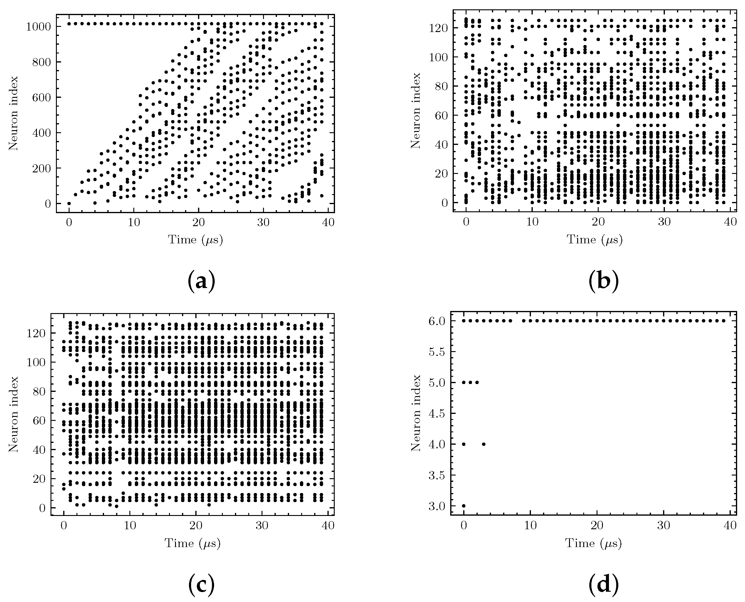
4.2. Recognition Effect Display

In order to visually display the data processing flow of the proposed method, Figure 5 shows the spike trains fired by the neurons in each layer of the improved SNNs when the seventh class of radar pulse train is input (the spurious pulse rate and the missing pulse rate are set to 0.3). Figure 5a–d show spike trains from the encoding layer, the first hidden layer, the second hidden layer, and the output layer, respectively. It can be seen from Figure 5a that since the local DTOA sequence of each pulse is used as input, the input spike trains show obvious regularity even in the presence of serious data noise. This demonstrates the improved method’s superior adaptability to data noise compared to using only the first-order DTOA as input (as indicated by spike trains corresponding to the maximum and minimum neuron indices in each time step in Figure 5a). In Figure 5b,c, each spiking neuron shows a certain spike-firing pattern, indicating that the spiking neuron has a specific response to the input timing pattern, and the response results are implicit in the timing structure of spike trains fired by different neurons. In Figure 5d, neurons corresponding to the correct class emit continuous spikes, whereas other neurons remain largely inactive, indicating that the network correctly recognizes the radar pulse train. Furthermore, spike-firing rates are calculated for Figure 5a–c, revealing rates of 0.015, 0.15, and 0.35 for the first, second, and third layers, respectively. These calculations indicate that the overall spike-firing rate of the SNNs is only 0.07, significantly reducing computational complexity.

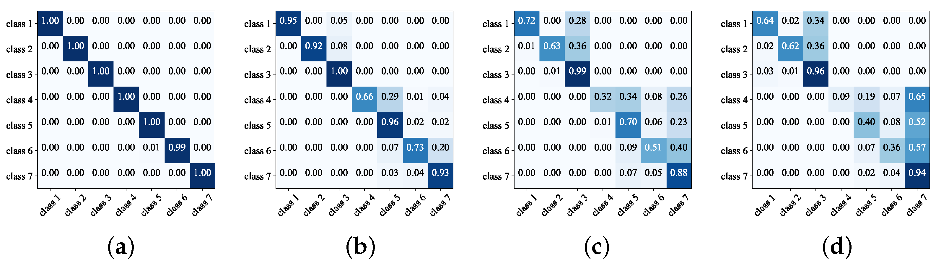
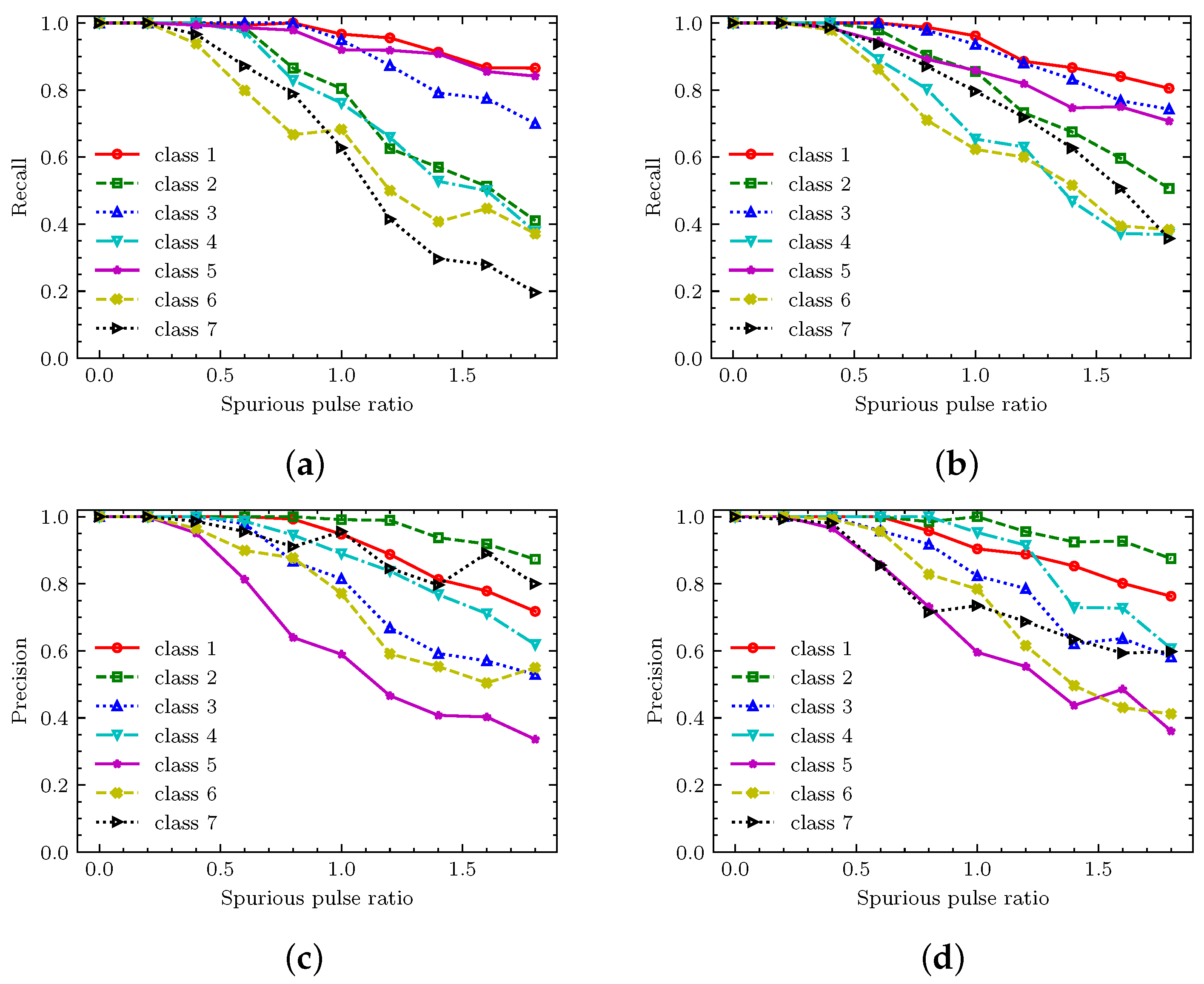
4.3. Recognition Performance Test of SNNs

The performance of the proposed SNNs is evaluated, and the confusion matrices under different missing pulse rates and spurious pulse rates are obtained, as shown in Figure 6. In Figure 6, the abscissa represents the predicted category label, and the ordinate represents the real category label. It can be seen from the figure that when the missing pulse rate is 0.1 and the spurious pulse rate is 0.2, the recognition probability of the proposed method for each category is close to 1, indicating that the proposed method has perfect recognition performance when the data noise is low. When the missing and spurious pulse rates gradually increase, the probability of false recognition gradually increases. This is because as the missing pulse rate and the spurious pulse rate increase, PRI features in the pulse stream are severely damaged, so patterns learned by the SNNs do not match timing patterns in the actual radar pulse train. The figure illustrates a progressive increase in the probability of the first and second classes being classified as the third class while also showing a gradual rise in misclassification of the fourth to sixth classes as the seventh class. This is because of the significant overlap in parameters within the first three classes and within the last four classes. Since the third and seventh classes have unique PRI values, they can be effectively distinguished from others. In addition, because the PW of the first three classes is significantly different from that of the last four classes, they can be effectively distinguished.
In order to evaluate the performance of the proposed method more comprehensively, the precision and recall of the method are tested when the missing pulse rate is 0.3 and 0.5, respectively, and the spurious pulse rate increases from 0 to 1.8. The test results are shown in Figure 7. Figure 7a,b, respectively, correspond to the recall when the missing pulse rate is fixed at 0.3 and 0.5 and the spurious pulse rate increases from 0 to 1.8. It can be seen from the figure that the recall of the proposed method is above 90% when the missing pulse rate and the spurious pulse rate are less than 0.5. As the spurious pulse rate increases, the recall gradually decreases. This is because the spurious pulse splits the original PRI pattern in the pulse stream, making it difficult to distinguish between different classes of pulse streams. When the missing pulse rate increases, the recall of most classes decreases slightly, while the recall of class 3 and class 7 increases slightly. This is because these two classes have unique PRIs compared to other classes, so they are easier to distinguish than other classes when serious data noise is present. Figure 7c,d correspond to the precision when the missing pulse rate is fixed at 0.3 and 0.5 and the spurious pulse rate increases from 0 to 1.8, respectively. As the spurious pulse rate increases, the precision of each class gradually decreases. When the missing pulse rate increases from 0.3 to 0.5, except for the seventh class, the precision of the other classes does not decrease significantly. This is because with the increase of data noise, classes 4 to 6 cannot be well distinguished from class 7, resulting in a significant increase in the number of pulse streams predicted as class 7, so that the precision of this class is reduced, which is similar to the results shown in the confusion matrix.

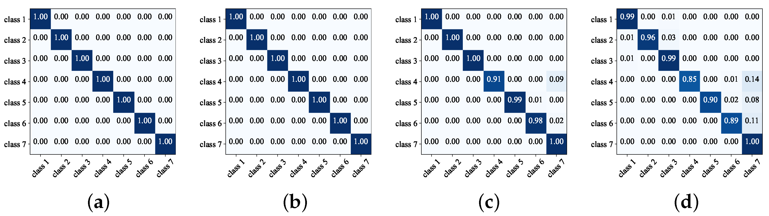
4.4. Recognition Performance Test of Improved SNNs

Figure 8 shows the confusion matrix of the improved SNNs under different missing pulse rates and spurious pulse rates. It can be seen from the figure that when the missing pulse rate is less than 0.8 and the spurious pulse rate is less than 1.4, the recognition probability of the proposed method for each class is close to 1. When the missing pulse rate is 0.8 and the spurious pulse rate is 1.4, the recognition probability of the proposed method for each category is still above 85%. In the case of very serious data noise in Figure 8d, due to the overlap of parameters, there are still false recognition results similar to Section 4.3, but the probability of false recognition is much smaller.
Figure 9 illustrates the proposed method’s precision and recall across varying missing and spurious pulse rates. Figure 9a,b demonstrate that when the spurious pulse rate is below 1.5, the recall for each class approaches 1. The recall for the first three classes is slightly higher for small missing pulse rates than others due to their simpler parameter patterns. As the missing pulse rate increases, classes 3 and 7 become more distinguishable from the rest due to their unique PRI features. However, due to overlapping PRI parameters, some radar pulse streams from classes 4 and 5 are misclassified as class 7, resulting in a slight decrease in recall. Figure 9c,d correspond to the precision under fixed missing pulse rates of 0.3 and 0.5, respectively, while varying the spurious pulse rate from 0 to 1.8. It can be seen from the figure that when the spurious pulse rate is less than 1.2, the precision of each class is close to 1. When the missing pulse rate increases from 0.3 to 0.5, except for the seventh class, other classes’ precision does not decrease significantly. This is because with the increase in data noise, classes 4 to 6 cannot be well distinguished from class 7, increasing the number of pulse streams predicted as class 7 in classes 4 to 6. By comparing with Section 4.3, it can be found that the proposed improved method has stronger data noise adaptability. These experimental findings demonstrate that using the local DTOA sequence of each pulse as PRI features effectively mitigates the impact of missing and spurious pulses on timing pattern integrity.

4.5. Performance Comparison of Different Methods

Finally, the recognition performance of our proposed method is compared with that of other common intelligent models under varying missing pulse rates and spurious pulse rates. In this section, LSTM [18], CNN [31,32], and MLP [33] are selected as comparison methods. The specific structures of SNNs, LSTM, and MLP are consistent with those in [15]. The CNN-based method is derived from [31,32]. PRI and PW features of each pulse are first transformed into embedded vectors, which are then concatenated along the time dimension. To facilitate CNN processing, pulse lengths are fixed at 20, and then a two-dimensional image of the same size is obtained. These images are input into a two-dimensional CNN and pooling layer for further processing, with final recognition results obtained via a fully connected layer. Throughout the comparison process, the same datasets and similar network structures are used to ensure an objective comparison. The comparison results are shown in Figure 10 and Figure 11. Figure 10 shows the recognition accuracy of different algorithms when the spurious pulse rate is fixed at 0.5 and the missing pulse rate increases from 0 to 0.8. Figure 11 mainly tests the accuracy of different algorithms when the missing pulse rate is fixed at 0.5 and the spurious pulse rate increases from 0 to 1.8. We set such a high missing pulse rate and spurious pulse rate to better verify the adaptability of our proposed method to a high missing pulse rate and high spurious pulse rate and the generalization performance of the algorithm when the electromagnetic environment changes.
It can be seen from Figure 10 that the accuracy of the proposed method is above 90% when the missing pulse rate increases from 0 to 0.8. Because the improved SNNs can avoid the split effect of data noise, the accuracy remains one under various missing pulse rates. For SNNs, the accuracy is unchanged when the missing pulse rate increases from 0 to 0.6. When the missing pulse rate is greater than 0.6, the recognition accuracy of this method begins to decline slowly, and the decline rate is smaller than that of the LSTM method. It can also be seen from the figure that the performance of the proposed method is better than that of the LSTM method as a whole and is much better than the other two methods.
It can be seen from Figure 11 that the accuracy of the proposed improved SNNs is close to 1 when the spurious pulse rate is less than 1.4. The accuracy of the proposed SNN-based method is more than 90% when the spurious pulse rate is less than 0.8, and the accuracy is slightly larger than that of the LSTM-based method under various spurious pulse rates, and the decline rate of the accuracy is much lower than that of the CNN-based and MLP-based methods. In addition, it can be found in Figure 10 and Figure 11 that the accuracy of MLP-based methods is very low since MLP does not have the processing power of time series data.
The results above indicate that the SNN-based method exhibits superior adaptability to data noise compared to LSTM. The experimental results further demonstrate that the improved SNN exhibits notable advancements in adapting to data noise by using the local timing structure of radar pulses. Moreover, the training datasets limit both missing and spurious pulse rates to [0, 0.5]. If these rates exceed this range significantly, the performance of the proposed methods exhibits a slower decline compared to other methods, indicating superior generalization capabilities.
Based on the experimental results above, we can analyze the reasons for the performance advantages of the proposed method as follows:
(1)
The voltage attenuation and threshold firing characteristics of SNNs effectively suppress data noise within the pulse stream.
(2)
The voltage accumulation characteristics of the SNN enable it to generate a continuously increasing response to the specific timing features in the pulse stream.
(3)
The proposed local timing structure of each pulse as a PRI feature is less affected by the splitting effect of data noise.

5. Discussion

By using the sequential processing ability of SNNs and the noise-insensitive timing features, the proposed method shows stronger data noise adaptability and generalization ability than existing methods. In this section, we further discuss computational efficiency of the proposed method and its applicability to more complex radar signal recognition.

5.1. Computational Efficiency Analysis

This subsection compares the computational complexity and real running time of SNNs and ANNs. The ANN model used for comparison is LSTM. Firstly, the number of additions and multiplications performed by the forward inference of SNNs and LSTM at each time step is calculated. For the lth layer of the network, the computational complexity of LSTM is 4 N l ( N l 1 + N l ) multiply-and-accumulate operations (MACs) [34]. According to Equation (14), the computational complexity of SNNs is ν N l N l 1 accumulate operations (ACs), where ν represents the average spike-firing rate of the ( l 1 )th layer. The voltage decay operation described in Equation (13), being intrinsic to spiking neurons, can be avoided in hardware implementations on specialized chips. Therefore, the lower computational complexity of SNNs comes from two aspects. The first is the sparsity of the spike trains in Equation (14). When the number of activated neurons is small, most of calculations can be avoided. The second comes from accumulate operations. When a new spike arrives, the voltage of the neuron is incremented by a specific value. In contrast, LSTM requires intensive multiplication for each neuron at each time step. Even considering the dynamics of spiking neurons in Equations (12), (13) and (15), the computational complexity of these equations is only proportional to N l and thus can be ignored compared with the computational complexity (proportional to N l N l 1 ). Additionally, the number of trainable parameters in the lth layer of SNNs is N l 1 N l , whereas LSTM, needing complex gates to enhance network performance, results in approximately eight times more parameters, around 4 [ N l ( N l 1 + N l ) + N l ] .
The energy consumption of SNNs and ANNs can also be further compared. When using a 45 nm CMOS process, a single-integer accumulate operation requires 0.1 pJ, while a multiply-and-accumulate operation requires 3.2 pJ. Through the simulation experiment observation, in general, the average spike-firing rate ν is about 0.1. In addition, a lower average spike-firing rate can be obtained by further setting the regularization term in the loss function. The analysis reveals that the energy consumption during the forward propagation of a specific layer in SNNs is merely 1/320 compared to an equivalent-sized ANN, rendering the proposed method more apt for resource-limited radar.
Then, we conduct further simulation experiments to verify the proposed method’s timeliness advantage. First, we input the first class of pulse train with a missing pulse rate and a spurious pulse rate of 0, including 40 pulses, into the proposed SNNs and LSTM. In order to fairly compare the performance of different methods, we tested the total time consumed by the proposed SNNs and LSTM with the same size of the hidden layer when processing pulses of different lengths. The running time is shown in Figure 12.
Figure 12 shows that the time the proposed SNNs consume in processing a single pulse is 0.14 ms, which is only about 1/3 of the LSTM-based method. In addition, it can be found that the processing time gap shown in the figure is not completely consistent with the results of the theoretical analysis. This is because only when the SNN runs on a specific neuromorphic chip can its event-driven addition computational efficiency tend to the theoretical value (at least 80 times faster than LSTM), thus providing the possibility for real-time recognition of radar pulse streams in complex environments.

5.2. Recognition of Multiple Radar Emitters in Interleaved Pulse Streams

The proposed method mainly recognizes a single radar emitter in a radar pulse stream with a large amount of data noise after deinterleaving. For an interleaved pulse stream, that is, a pulse stream in which there are pulses from multiple radar emitters, the proposed method needs to be further improved due to the mutual interference of pulses from different emitters.
The proposed method has the following difficulties when applied to recognition of interleaved pulse streams. Firstly, PRI features of pulses from a single radar in an interleaved pulse stream are severely split by pulses from other radars, making it difficult for the proposed method to distinguish PRI features of pulses from different radars effectively. Secondly, the time interval pattern between two adjacent pulses from a single radar in an interleaved pulse stream varies greatly under different data conditions, which makes it difficult for the proposed SNNs to generate stable responses to different data conditions. Moreover, since the loss function used in this paper is mainly used for single-label multiclassification, it is difficult to be applied to recognize multiple emitters (it is a multilabel multiclassification problem).
In future research, the proposed method can be optimized in the following aspects to adapt to the recognition of radar emitters in an interleaved pulse stream:
(1)
PRI features that can more effectively distinguish the pulses from different radar emitters should be adopted. For example, the hidden state of the temporal feature self-supervised learning network can be used as PRI features of pulses [13], and then the direct coding method in this paper can be used to encode it into spike trains that SNNs can process.
(2)
The TOA of each pulse, rather than time step, should be directly used as the time dimension of each pulse. By changing the proposed method to an event-driven form, the network can directly use the TOA of each pulse as a time dimension, thereby generating a more stable response to the pulse stream from a specific radar.
(3)
The proposed network should be changed to a multilabel multiclassification form. This includes changing the original cross-entropy loss function to a binary cross-entropy loss function. Moreover, the process of network training needs to be optimized, that is, the model is required to be able to handle the correlation and overlap between data belonging to different labels, which involves more complex training and evaluation processes.

5.3. Recognition of More Complex Aliasing Radar Signals

The proposed method is mainly based on the inter-pulse features of the radar pulse stream (i.e., PDW sequence) to recognize radar emitters. However, when signals from different radars are highly overlapped in the time domain and frequency domain (e.g., aliasing LPI radar signals [35] and FMCW signals [36]), the proposed method is no longer applicable. This is because PDWs of these signals cannot be accurately measured or these radar signals cannot be effectively distinguished by PDWs. In this case, it is necessary to use intra-pulse features to recognize aliasing radar signals.
There are also a small number of intra-pulse modulation signal recognition methods based on SNNs. In [26], Alex et al. proposed an LPI radar waveform recognition method based on spiking convolutional neural networks (SCNNs). Before classification, the Choi–Williams distribution (CWD) is used to analyze LPI radar signals to obtain time–frequency images, and then the multilayer spiking convolution block is used to encode and classify time–frequency images. Li et al. [37] first used the Born–Jordan distribution to transform intercepted radar signals into two-dimensional time–frequency images and then used rate coding to convert the single pixel value of each image into spike trains. Finally, a three-layer fully connected SNN is used to recognize intra-pulse modulation types of intercepted radar signals. Although the above method can process intra-pulse modulation signals, there are two obvious problems. Firstly, the above methods only solve the problem of single radar emitter recognition and cannot be used for overlapping radar signals. Secondly, the above methods use SNNs to realize static image recognition and do not make full use of the sequential processing ability of SNNs.
In view of the above problems, we propose two SNN-based aliased radar pulse stream recognition ideas: (1) The intercepted radar signal is firstly transformed into a time–frequency image and encoded into spike trains, and then multiple binary SNNs [38] are established to realize the recognition of multiple radar emitters in the aliasing pulse stream. (2) Considering that the waveform of the radar signal is similar to that of the ECG signal, the radar signal in the time domain can be directly transformed into spike trains by level-crossing sampling [39], and then a spiking recursive MLP can be established to classify it [40]. In network training, the binary cross entropy is used as the loss function, and SNNs for recognizing different radar signals in the aliasing pulse stream are trained based on the STBP algorithm mentioned in this paper. In the above process, encoding and recognition can be carried out online to make full use of the sequential processing ability and computational efficiency of SNNs. In general, aliasing radar signal recognition based on SNNs is a feasible and valuable research direction.

6. Conclusions

This paper proposes a radar emitter recognition method based on SNNs. Firstly, a lightweight SNN for radar emitter recognition is established. Then, by introducing the local timing structure of pulses, we further propose a radar emitter recognition method based on an improved SNN with stronger data noise adaptability and lower computational complexity. Finally, the proposed method realizes effective and efficient radar emitter recognition under complex data conditions. The simulation results are as follows:
(1)
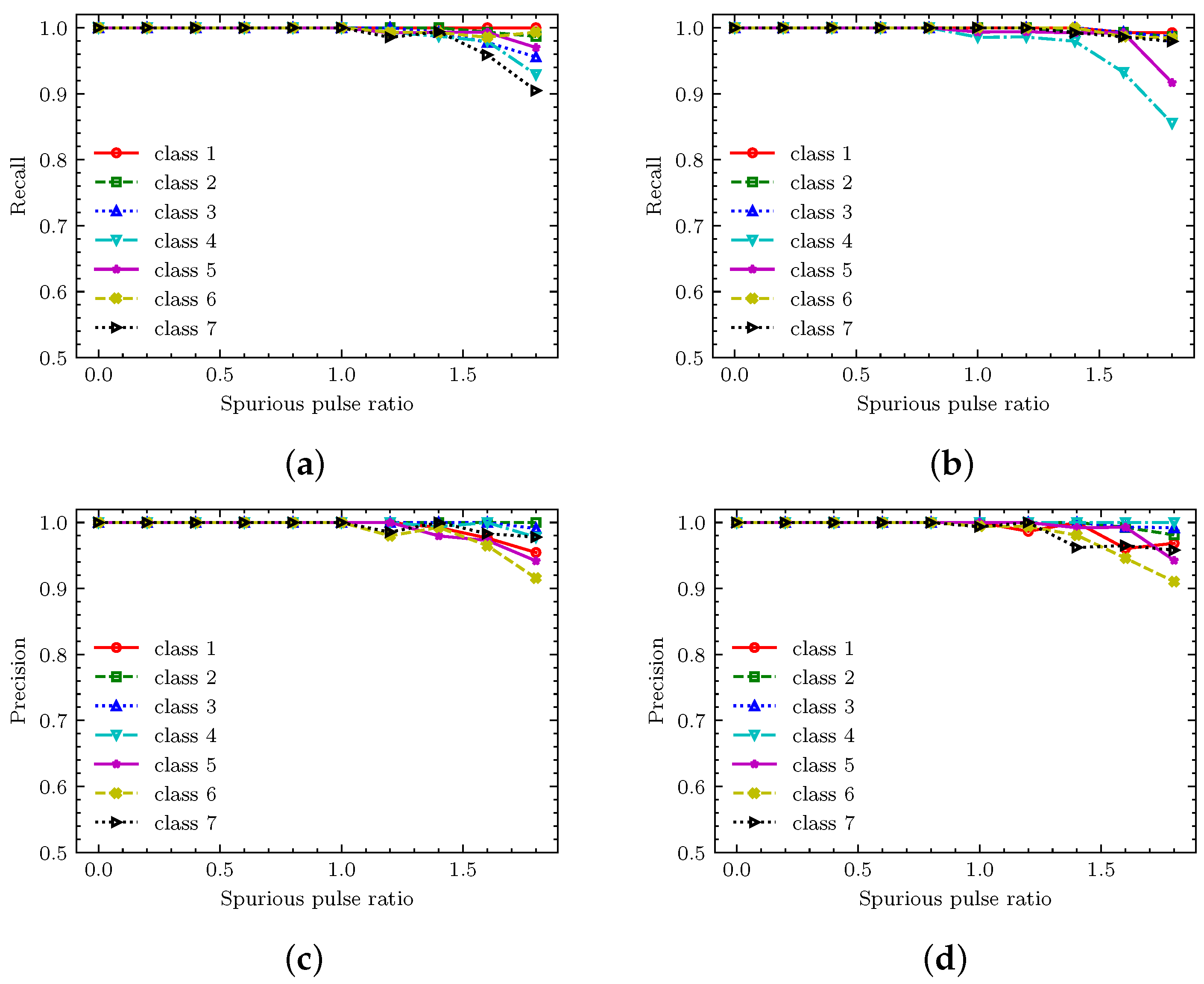
The proposed SNN-based method has a recall and precision of more than 90% for all classes of radars when the spurious pulse rate and missing pulse rate do not exceed 0.5.
(2)
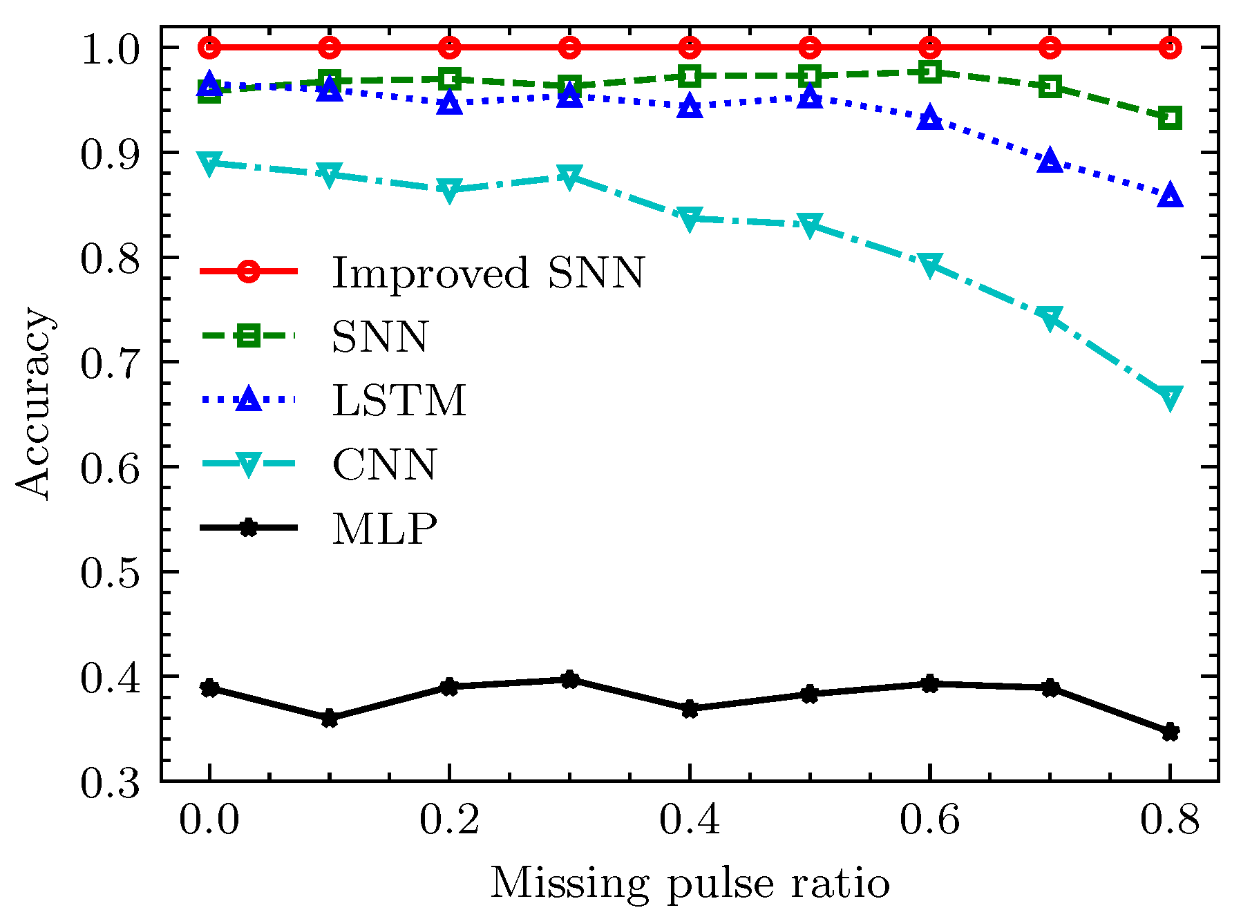
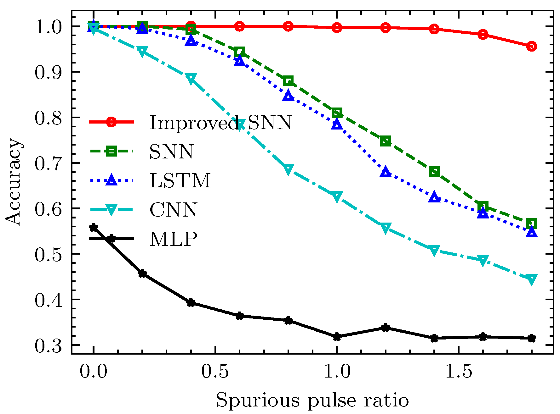
Compared with missing pulses, spurious pulses have a greater impact on the recognition accuracy of the SNN-based method. This is because when there is a spurious pulse, the PRI feature of its adjacent pulses is randomly split, resulting in SNNs being unable to generate an effective response.
(3)
Compared with other methods, the proposed SNN-based method has stronger data noise adaptability. The reason is that the voltage attenuation, spike-firing, and voltage accumulation characteristics of SNNs can effectively suppress the data noise in the pulse stream while retaining the effective features of the radar pulse stream.
(4)
Recall and precision for each class in the improved method are still more than 90% when the missing pulse rate is 0.5 and the spurious pulse rate is 1.8. Moreover, the improved SNNs have significantly higher adaptability to data noise than other methods. This is because the local timing features are less affected by data noise, especially spurious pulses, so they can generate a more stable response to specific timing patterns in the pulse stream.
(5)
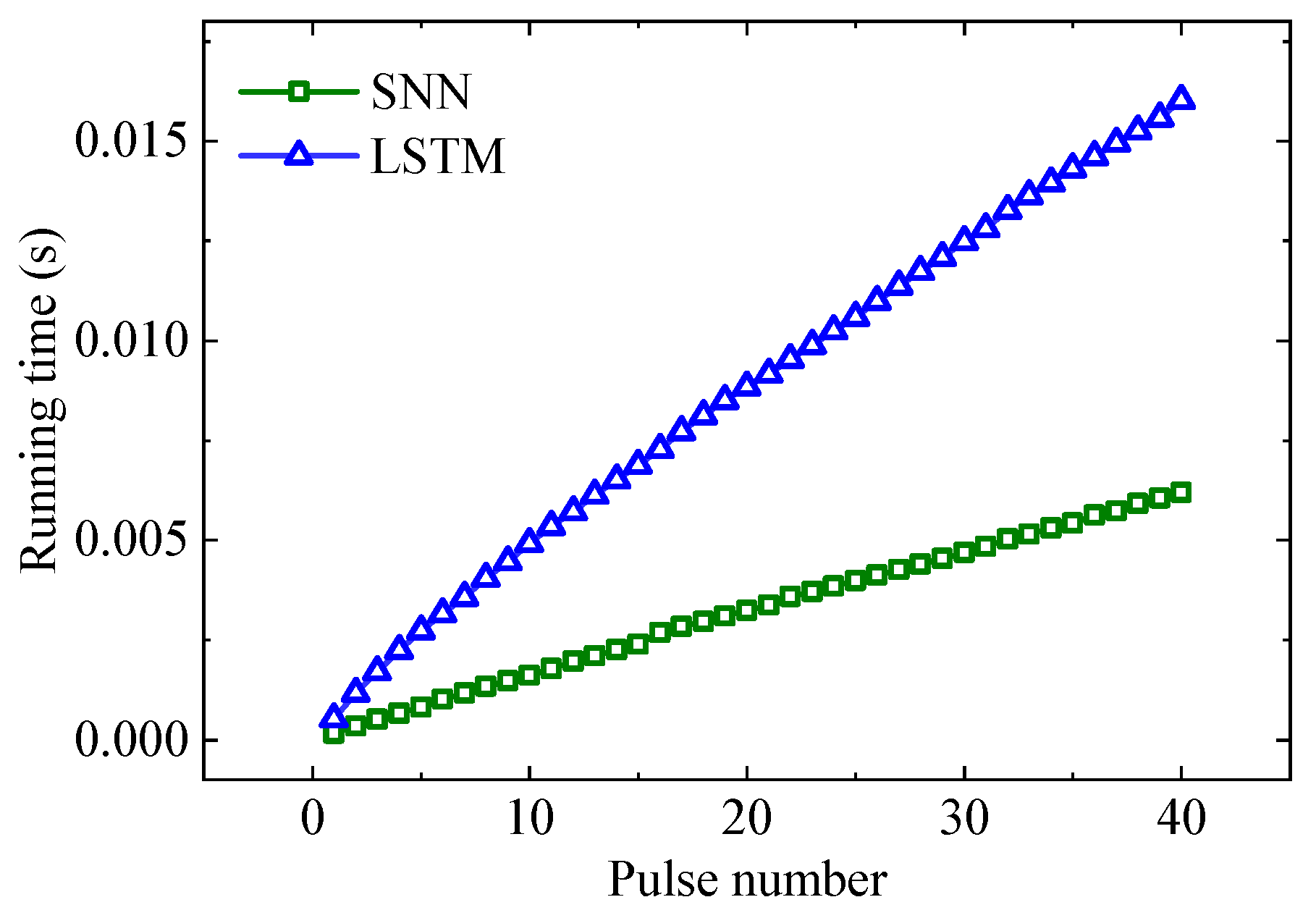
The computational complexity analysis and simulation experiments of the proposed method show that the proposed method also has higher computational efficiency and provides the possibility for real-time recognition of radar pulse streams under complex signal conditions.

Author Contributions

Conceptualization, Z.L. (Zhenghao Luo) and Z.L. (Zhangmeng Liu); data curation, Z.L. (Zhenghao Luo), X.W. and S.Y.; methodology, Z.L. (Zhenghao Luo); supervision, Z.L. (Zhangmeng Liu); writing—original draft, Z.L. (Zhenghao Luo); writing—review and editing, X.W., S.Y. and Z.L. (Zhangmeng Liu). All authors have read and agreed to the published version of the manuscript.

Funding

The work was supported by National Natural Science Foundation of China, Grant/Award Number: 62371456.

Data Availability Statement

Data is contained within the article.

Conflicts of Interest

The authors declare no conflicts of interest.

Abbreviations

The following abbreviations are used in this manuscript:
AbbreviationsFull NamesDescriptions
ESMElectronic support measurementIt is used to detect, locate, and identify radar to provide knowledge for an electronic countermeasure system.
SNNSpiking neural networkA third-generation neural network which can more realistically simulate the biological brain neurons.
ANNArtificial neural networkThe second generation of neural networks using traditional neurons, such as RNN and CNN.
LSTMLong short-term memoryA deep learning model commonly used to process and predict time series data.
CNNConvolutional neural networkA deep learning model for processing and analyzing data with spatial structure.
MLPMultilayer perceptronA basic feedforward neural network model, usually composed of multiple fully connected layers.
LIFLeaky integrate-and-fireA low-computational-complexity spiking neuron model.
PDWPulse description wordA digital descriptor composed of all parameters of a single radar pulse.
TOATime of arrival
PWPulse width
RFRadio frequency
DOADirection of arrival
DTOADifferential time of arrivalThe time interval between two adjacent pulses of an intercepted pulse stream.
PRIPulse repetition intervalThe time interval between two adjacent pulses emitted by the radar.
MFRMultifunction radarA radar system capable of performing multiple radar tasks.
LPILow probability of intercept radarA radar system designed to reduce the likelihood of detection by electronic reconnaissance systems.
FMCWFrequency modulated continuous wave radarA radar technology based on continuously transmitting and receiving frequency-modulated continuous wave signals.
MSEMean square error
LTSLocal timing structureNoise-insensitive PRI feature proposed in this paper.
MACsMultiply-and-accumulate operations
ACsAccumulate operations

References

  1. Wiley, R.G. ELINT: The Interception and Analysis of Radar Signals; Artech House Radar Library, Artech House: Boston, MA, USA, 2006. [Google Scholar]
  2. Luo, Z.; Yuan, S.; Shang, W.; Liu, Z. Automatic Reconstruction of Radar Pulse Repetition Pattern Based on Model Learning. Digit. Signal Process. 2024, 152, 104596. [Google Scholar] [CrossRef]
  3. Jing, Z.; Li, P.; Wu, B.; Yan, E.; Chen, Y.; Gao, Y. Attention-Enhanced Dual-Branch Residual Network with Adaptive L-Softmax Loss for Specific Emitter Identification under Low-Signal-to-Noise Ratio Conditions. Remote Sens. 2024, 16, 1332. [Google Scholar] [CrossRef]
  4. Yuan, S.; Li, P.; Wu, B. Radar Emitter Signal Intra-Pulse Modulation Open Set Recognition Based on Deep Neural Network. Remote Sens. 2023, 16, 108. [Google Scholar] [CrossRef]
  5. Dash, D.; Valarmathi, J. Radar Emitter Identification in Multistatic Radar System: A Review. In Advances in Automation, Signal Processing, Instrumentation, and Control; Komanapalli, V.L.N., Sivakumaran, N., Hampannavar, S., Eds.; Springer Nature: Singapore, 2021; Volume 700, pp. 2655–2664. [Google Scholar] [CrossRef]
  6. Xu, T.; Yuan, S.; Liu, Z.; Guo, F. Radar Emitter Recognition Based on Parameter Set Clustering and Classification. Remote Sens. 2022, 14, 4468. [Google Scholar] [CrossRef]
  7. Liangliang, G.; Shilong, W.; Tao, L. A Radar Emitter Identification Method Based on Pulse Match Template Sequence. In Proceedings of the 2010 2nd International Conference on Signal Processing Systems, Dalian, China, 5–7 July 2010; pp. V3-153–V3-156. [Google Scholar] [CrossRef]
  8. Kvasnov, A.V.; Shkodyrev, V.P.; Arsenyev, D.G. Method of Recognition the Radar Emitting Sources Based on the Naive Bayesian Classifier. WSEAS Trans. Syst. Control 2019, 14, 112–120. [Google Scholar]
  9. Revillon, G.; Mohammad-Djafari, A.; Enderli, C. Radar Emitters Classification and Clustering with a Scale Mixture of Normal Distributions. IET Radar Sonar Navig. 2019, 13, 128–138. [Google Scholar] [CrossRef]
  10. Chen, W.; Fu, K.; Zuo, J.; Zheng, X.; Huang, T.; Ren, W. Radar Emitter Classification for Large Data Set Based on Weighted-xgboost. IET Radar Sonar Navig. 2017, 11, 1203–1207. [Google Scholar] [CrossRef]
  11. Shieh, C.S.; Lin, C.T. A Vector Neural Network for Emitter Identification. IEEE Trans. Antennas Propag. 2002, 50, 1120–1127. [Google Scholar] [CrossRef]
  12. Chen, Y.; Li, P.; Yan, E.; Jing, Z.; Liu, G.; Wang, Z. A Knowledge Graph-Driven CNN for Radar Emitter Identification. Remote Sens. 2023, 15, 3289. [Google Scholar] [CrossRef]
  13. Yuan, S.; Liu, Z.M. Temporal Feature Learning and Pulse Prediction for Radars with Variable Parameters. Remote Sens. 2022, 14, 5439. [Google Scholar] [CrossRef]
  14. Wang, J.; Wang, H.; Xu, K.; Mao, Y.; Xuan, Z.; Tang, B.; Wang, X.; Mu, X. Visualization and Classification of Radar Emitter Pulse Sequences Based on 2D Feature Map. Phys. Commun. 2023, 61, 102168. [Google Scholar] [CrossRef]
  15. Liu, Z.M.; Philip, S.Y. Classification, Denoising, and Deinterleaving of Pulse Streams with Recurrent Neural Networks. IEEE Trans. Aerosp. Electron. Syst. 2019, 55, 1624–1639. [Google Scholar] [CrossRef]
  16. Notaro, P.; Paschali, M.; Hopke, C.; Wittmann, D.; Navab, N. Radar Emitter Classification with Attribute-specific Recurrent Neural Networks. arXiv 2019, arXiv:1911.07683. [Google Scholar] [CrossRef]
  17. Li, X.; Liu, Z.; Huang, Z.; Liu, W. Radar Emitter Classification with Attention-Based Multi-RNNs. IEEE Commun. Lett. 2020, 24, 2000–2004. [Google Scholar] [CrossRef]
  18. Li, Y.; Zhu, M.; Ma, Y.; Yang, J. Work Modes Recognition and Boundary Identification of MFR Pulse Sequences with a Hierarchical Seq2seq LSTM. IET Radar Sonar Navig. 2020, 14, 1343–1353. [Google Scholar] [CrossRef]
  19. Zhang, Z.; Zhu, M.; Li, Y.; Li, Y.; Wang, S. Joint Recognition and Parameter Estimation of Cognitive Radar Work Modes with LSTM-transformer. Digit. Signal Process. 2023, 140, 104081. [Google Scholar] [CrossRef]
  20. Venkataramani, S.; Roy, K.; Raghunathan, A. Efficient Embedded Learning for IoT Devices. In Proceedings of the 2016 21st Asia and South Pacific Design Automation Conference (ASP-DAC), Macao, China, 25–28 January 2016; pp. 308–311. [Google Scholar] [CrossRef]
  21. Liu, Y.; Tian, M.; Liu, R.; Cao, K.; Wang, R.; Wang, Y.; Zhao, W.; Zhou, Y. Spike-Based Approximate Backpropagation Algorithm of Brain-Inspired Deep SNN for Sonar Target Classification. Comput. Intell. Neurosci. 2022, 2022, 1633946. [Google Scholar] [CrossRef]
  22. Maass, W. Networks of Spiking Neurons: The Third Generation of Neural Network Models. Neural Netw. 1997, 10, 1659–1671. [Google Scholar] [CrossRef]
  23. Wu, Y.; Deng, L.; Li, G.; Zhu, J.; Shi, L. Spatio-Temporal Backpropagation for Training High-Performance Spiking Neural Networks. Front. Neurosci. 2018, 12, 331. [Google Scholar] [CrossRef]
  24. He, W.; Wu, Y.; Deng, L.; Li, G.; Wang, H.; Tian, Y.; Ding, W.; Wang, W.; Xie, Y. Comparing SNNs and RNNs on Neuromorphic Vision Datasets: Similarities and Differences. Neural Netw. 2020, 132, 108–120. [Google Scholar] [CrossRef]
  25. Bittar, A.; Garner, P.N. A Surrogate Gradient Spiking Baseline for Speech Command Recognition. Front. Neurosci. 2022, 16, 865897. [Google Scholar] [CrossRef] [PubMed]
  26. Henderson, A.; Harbour, S.; Yakopcic, C.; Taha, T.; Brown, D.; Tieman, J.; Hall, G. Spiking Neural Networks for LPI Radar Waveform Recognition with Neuromorphic Computing. In Proceedings of the 2023 IEEE Radar Conference (RadarConf23), San Antonio, TX, USA, 1–5 May 2023; pp. 1–6. [Google Scholar] [CrossRef]
  27. Roy, K.; Jaiswal, A.; Panda, P. Towards Spike-Based Machine Intelligence with Neuromorphic Computing. Nature 2019, 575, 607–617. [Google Scholar] [CrossRef] [PubMed]
  28. Yi, Z.; Lian, J.; Liu, Q.; Zhu, H.; Liang, D.; Liu, J. Learning Rules in Spiking Neural Networks: A Survey. Neurocomputing 2023, 531, 163–179. [Google Scholar] [CrossRef]
  29. Wu, Y.; Deng, L.; Li, G.; Zhu, J.; Shi, L. Direct Training for Spiking Neural Networks: Faster, Larger, Better. arXiv 2018, arXiv:1809.05793. [Google Scholar] [CrossRef]
  30. Kim, Y.; Park, H.; Moitra, A.; Bhattacharjee, A.; Venkatesha, Y.; Panda, P. Rate Coding Or Direct Coding: Which One Is Better For Accurate, Robust, And Energy-Efficient Spiking Neural Networks? In Proceedings of the ICASSP 2022—2022 IEEE International Conference on Acoustics, Speech and Signal Processing (ICASSP), Singapore, 23–27 May 2022; pp. 71–75. [Google Scholar] [CrossRef]
  31. Li, X.; Huang, Z.; Wang, F.; Wang, X.; Liu, T. Toward Convolutional Neural Networks on Pulse Repetition Interval Modulation Recognition. IEEE Commun. Lett. 2018, 22, 2286–2289. [Google Scholar] [CrossRef]
  32. Al-Malahi, A.; Farhan, A.; Feng, H.; Almaqtari, O.; Tang, B. An Intelligent Radar Signal Classification and Deinterleaving Method with Unified Residual Recurrent Neural Network. IET Radar Sonar Navig. 2023, 17, 1259–1276. [Google Scholar] [CrossRef]
  33. Petrov, N.; Jordanov, I.; Roe, J. Radar Emitter Signals Recognition and Classification with Feedforward Networks. Procedia Comput. Sci. 2013, 22, 1192–1200. [Google Scholar] [CrossRef]
  34. Yin, B.; Corradi, F.; Bohté, S.M. Accurate and Efficient Time-Domain Classification with Adaptive Spiking Recurrent Neural Networks. Nat. Mach. Intell. 2021, 3, 905–913. [Google Scholar] [CrossRef]
  35. Pan, Z.; Wang, S.; Li, Y. Residual Attention-Aided U-Net GAN and Multi-Instance Multilabel Classifier for Automatic Waveform Recognition of Overlapping LPI Radar Signals. IEEE Trans. Aerosp. Electron. Syst. 2022, 58, 4377–4395. [Google Scholar] [CrossRef]
  36. Chen, K.; Zhang, J.; Chen, S.; Zhang, S.; Zhao, H. Recognition and Estimation for Frequency-Modulated Continuous-Wave Radars in Unknown and Complex Spectrum Environments. IEEE Trans. Aerosp. Electron. Syst. 2023, 59, 6098–6111. [Google Scholar] [CrossRef]
  37. Wei, L.; Wei-gang, Z.; Hong-feng, P.; Hong-yu, Z. Radar Emitter Identification Based on Fully Connected Spiking Neural Network. J. Phys. Conf. Ser. 2021, 1914, 012036. [Google Scholar] [CrossRef]
  38. Xiao, R.; Tang, H.; Gu, P.; Xu, X. Spike-Based Encoding and Learning of Spectrum Features for Robust Sound Recognition. Neurocomputing 2018, 313, 65–73. [Google Scholar] [CrossRef]
  39. Saeed, M.; Wang, Q.; Martens, O.; Larras, B.; Frappe, A.; Cardiff, B.; John, D. Evaluation of Level-Crossing ADCs for Event-Driven ECG Classification. IEEE Trans. Biomed. Circuits Syst. 2021, 15, 1129–1139. [Google Scholar] [CrossRef]
  40. Chu, H.; Yan, Y.; Gan, L.; Jia, H.; Qian, L.; Huan, Y.; Zheng, L.; Zou, Z. A Neuromorphic Processing System with Spike-Driven SNN Processor for Wearable ECG Classification. IEEE Trans. Biomed. Circuits Syst. 2022, 16, 511–523. [Google Scholar] [CrossRef] [PubMed]
Figure 1. Comparison of spiking neural networks and artificial neural networks. Information processing diagram of (a) spiking neural networks and (b) artificial neural networks.
Remotesensing 16 02680 g001
Figure 2. Radar pulse train diagram. (a) The original pulse stream without data noise. (b) Intercepted radar pulse train with three common data noises.
Remotesensing 16 02680 g002
Figure 3. SNN structure for radar emitter recognition. The digitized PRI and PW are first transformed into one-hot vectors, then embedded into lower dimensional features and concatenated, and then encoded into spike trains through the encoding layer. Finally, spiking neurons in the output layer corresponding to the correct category have the highest spike firing rate.
Remotesensing 16 02680 g003
Figure 4. Structure of improved SNNs. Firstly, the local timing structure ( L t ) and pulse width of each pulse are encoded into spike trains. After the SNN processing, the spiking neuron corresponding to the correct class has the highest spike-firing rate in the output layer.
Remotesensing 16 02680 g004
Figure 5. Radar pulse train recognition experiment. (a) Spike trains fired by neurons in the encoding layer. (b) Spike trains fired by neurons in the first hidden layer. (c) Spike trains fired by neurons in the second hidden layer. (d) Spike trains fired by neurons in the output layer.
Remotesensing 16 02680 g005
Figure 6. Confusion matrix of radar emitter recognition based on SNNs. (a) Missing pulse rate is 0.1 and spurious pulse rate is 0.2. (b) Missing pulse rate is 0.3 and spurious pulse rate is 0.6. (c) Missing pulse rate is 0.5 and spurious pulse rate is 1.0. (d) Missing pulse rate is 0.7 and spurious pulse rate is 1.4.
Remotesensing 16 02680 g006
Figure 7. Recognition performance based on SNNs for different spurious pulse rates and missing pulse rates: (a,c) show recall and precision with a fixed missing pulse rate equal to 0.3 and varying spurious pulse rate from 0 to 1.8, while (b,d) show recall and precision with a fixed missing pulse rate equal to 0.5 and varying spurious pulse rate from 0 to 1.8.
Remotesensing 16 02680 g007
Figure 8. Confusion matrix of radar emitter recognition based on improved SNNs. (a) Missing pulse rate is 0.1, spurious pulse rate is 0.2. (b) Missing pulse rate is 0.3, spurious pulse rate is 0.6. (c) Missing pulse rate is 0.5, spurious pulse rate is 1.0. (d) Missing pulse rate is 0.7, spurious pulse rate is 1.4.
Remotesensing 16 02680 g008
Figure 9. Recognition performance based on improved SNNs for different spurious pulse rates and missing pulse rates: (a,c) show recall and precision with a fixed missing pulse rate equal to 0.3 and varying spurious pulse rate from 0 to 1.8, while (b,d) show recall and precision with a fixed missing pulse rate equal to 0.5 and varying spurious pulse rate from 0 to 1.8.
Remotesensing 16 02680 g009
Figure 10. The recognition accuracy under different missing pulse rates.
Remotesensing 16 02680 g010
Figure 11. The recognition accuracy under different spurious pulse rates.
Remotesensing 16 02680 g011
Figure 12. The running time of different methods when dealing with pulse streams with different lengths.
Remotesensing 16 02680 g012
Table 1. Parameters of 7 types of simulated radars.
ClassPW Mean ( μ s)PRI TypePRI Mean ( μ s)
12constant175
22constant200
32stagger[175, 200]
43stagger[175, 200]
53stagger[175, 200, 220]
63stagger[175, 200, 220, 250]
73stagger[175, 200, 220, 250, 320]
Disclaimer/Publisher’s Note: The statements, opinions and data contained in all publications are solely those of the individual author(s) and contributor(s) and not of MDPI and/or the editor(s). MDPI and/or the editor(s) disclaim responsibility for any injury to people or property resulting from any ideas, methods, instructions or products referred to in the content.

