Article

Digital Mapping and Scenario Prediction of Soil Salinity in Coastal Lands Based on Multi-Source Data Combined with Machine Learning Algorithms

1
Institute of Geographic Sciences and Natural Resources Research, Chinese Academy of Sciences, 11A Datun Road, Chaoyang District, Beijing 100101, China
2
University of Chinese Academy of Sciences, Beijing 100049, China
*
Author to whom correspondence should be addressed.
Remote Sens. 2024, 16(14), 2681; https://doi.org/10.3390/rs16142681 (registering DOI)
Submission received: 6 May 2024 / Revised: 13 June 2024 / Accepted: 19 July 2024 / Published: 22 July 2024

Abstract

:
Salinization is a major soil degradation process threatening ecosystems and posing a great challenge to sustainable agriculture and food security worldwide. This study aimed to evaluate the potential of state-of-the-art machine learning algorithms in soil salinity (EC1:5) mapping. Further, we predicted the distribution patterns of soil salinity under different future scenarios in the Yellow River Delta. A geodatabase comprising 201 soil samples and 19 conditioning factors (containing data based on remote sensing images such as Landsat, SPOT/VEGETATION PROBA-V, SRTMDEMUTM, Sentinel-1, and Sentinel-2) was used to compare the predictive performance of empirical bayesian kriging regression, random forest, and CatBoost models. The CatBoost model exhibited the highest performance with both training and testing datasets, with an average MAE of 1.86, an average RMSE of 3.11, and an average R2 of 0.59 in the testing datasets. Among explanatory factors, soil Na was the most important for predicting EC1:5, followed by the normalized difference vegetation index and soil organic carbon. Soil EC1:5 predictions suggested that the Yellow River Delta region faces severe salinization, particularly in coastal zones. Among three scenarios with increases in soil organic carbon content (1, 2, and 3 g/kg), the 2 g/kg scenario resulted in the best improvement effect on saline–alkali soils with EC1:5 > 2 ds/m. Our results provide valuable insights for policymakers to improve saline–alkali land quality and plan regional agricultural development.

1. Introduction

Soil salinization is a severe soil-health problem, as it poses a threat to crop growth, food security, and population mobility [1,2]. Unfortunately, saline–alkali land covers a vast expanse worldwide. According to the report released by the Food and Agriculture Organization of the United Nations (FAO) in 2021, the global area of saline soil exceeds 833 million hectares, and, in recent decades, China has been the country with the largest area of salinity-affected soils, with 211 million hectares, followed by Australia with 131 [3]. In addition, as noted by Hassani et al., 2021, climate change poses a greater risk of salinity in the Southern Hemisphere [4].
The spatial heterogeneity of soil physicochemical characteristics can be explained by conditions related to soil formation such as terrain, climate, land use, vegetation, and type of soil parent material. All these factors affect the distribution of soil salinity. For instance, factors such as altitude, slope orientation, temperature, precipitation, evaporation, and vegetation coverage can all influence the distribution of soil salinity [5,6]. Among the effective factors, the strongest controls on salinity are related to soil, terrain, and topographic characteristics [5]. Additionally, the vegetation index time-series has greatly contributed to large-scale soil salinity mapping [7]. Soil electrical conductivity (EC) is an important indicator of soil salinity, and Hassani et al. (2020) found that soil classification, depth, and fraction of absorbed photosynthetically active radiation are the most important predictors of the electrical conductivity of a saturated soil paste extract (ECe). Indeed, the factors influencing the distribution of soil EC can vary significantly across different regions. Therefore, identifying the key driving factors that affect EC distribution in the Yellow River Delta region is crucial for the design and implementation of effective soil-improvement strategies in this area.
Previously, the distribution of soil salinity in any given area was determined based on extensive field sampling, which is labor-intensive and time consuming [8]. The ability of remote sensing images to cover extensive areas and rapidly acquire large amounts of data over long periods has garnered significant scholarly attention. Among various methods, infrared spectroscopy is the most extensively employed technique and has been widely used for the spatial prediction and mapping of soil salinity [9,10]. However, despite these advancements, the low spatial resolution of remote sensing images caused by cloud interference, combined with the inherent complexity and heterogeneity of soil, presents significant challenges for the accurate interpretation of remote sensing data [11]. In recent years, artificial intelligence (AI) has gained prominence, and many machine learning models, especially the random forest (RF) model, have shown great potential for digital soil mapping and soil-attribute spatial prediction [12,13,14,15,16,17]. CatBoost is a novel gradient-boosting decision tree. Its main advantage is that it can efficiently and reasonably process categorical variables [18]. It is superior to XGBoost and LightGBM in terms of algorithm speed and accuracy for some benchmarks [19]. CatBoost has been used for medical evaluations and economic, engineering, and environmental predictions [20,21,22,23]. However, very few studies have used CatBoost to predict soil salinity. Thus, this study aimed to conduct a comparative analysis of the efficacy of geostatistical interpolation methods, namely Empirical Bayesian Kriging (EBK) regression prediction, relative to machine learning models, such as RF and CatBoost, in predicting soil EC.
The Yellow River Delta is the youngest wetland ecosystem in the world, and typically representative of saline–alkali land [24]. This wetland serves as an “international transfer station” for bird migration in Northeast Asia and the Pacific Rim, and is an important location for species protection, wetland management, migratory bird migration, and ecological succession research in river mouths. Affected by various hydrodynamic factors, such as the Yellow River and the Bohai Sea, this area has shallow groundwater (averaging approximately 1.14 m), high salinity levels (averaging approximately 14.3 g/L), and severe soil salinization [25]. These conditions severely limit the potential of this area. Therefore, knowledge of the spatial distribution of soil salinity in the Yellow River Delta is vital for improving saline–alkali land and planning agricultural development. In response to the severe problem of soil salinization, various mitigation strategies have been proposed, including straw covering, the application of organic fertilizers, and the use of biochar. Numerous studies have demonstrated that the addition of organic carbon can alleviate soil salinization [26,27,28,29]. Thus, it is pertinent to investigate the improvement effect of different organic carbon additions on soil salinity in the Yellow River Delta region. Determining the optimal amount of organic carbon needed to achieve the best amelioration effect remains an intriguing question for further research.
This study aimed to accurately map soil salinity distribution by combining geostatistical models, namely EBK regression prediction, with machine learning models, such as RF and CatBoost. The predictions are based on multi-source data including meteorological, RS, and soil property data. The objectives of this study were to (1) establish the optimal model for accurately predicting soil salinity in coastal saline–alkali soils in the region of the Yellow River Delta, (2) identify the important factors affecting the distribution of soil salinity in the region, (3) draw the spatial distribution map of soil salinity in the region and classify and quantify the saline soil in the region, and (4) explore and establish cost-effective measures to improve the quality of saline–alkali soils in the Yellow River Delta region. This study provided a scientific basis for the efficient utilization of coastal saline–alkali soils and sustainable development of regional agriculture.

2. Materials and Methods

2.1. Study Area

The study area (117°31′E–119°19′E, 37°04′N–38°16′N) is located on the west coast of the Bohai Sea and along the Yellow River estuary (Figure 1). The Yellow River Delta is the youngest wetland ecosystem in the world. Its unique geography is formed by the interactions among rivers, sea, and land. In 1855, the Yellow River (the fifth longest river in the world) was diverted through the Yellow and Bohai seas. This created an alluvial fan with a binary facies structure, in which river sediments covered a marine layer owing to the swing and deposition at the estuary end [30].
The Yellow River Delta has a warm temperate monsoon continental climate with hot and rainy seasons [31]. It has an annual average temperature of 12.2 °C and the interannual precipitation is unstable, with precipitation exceeding 900 mm in years with more rainfall and less than 400 mm in years with less rainfall [24]. Annual evaporation exceeds rainfall in the region, which causes an upward migration of salt in the soil, resulting in seasonal salt return and desalination. The main pattern observed in the area comprises salt accumulation in spring, desalination in summer, recovery in autumn, and incubation in winter [24]. The soil types are solonchaks and fluvo-aquic soils, which account for 80% of the total area [30].

2.2. Field Sampling and Soil Sample Analysis

A total of 201 topsoil (0–20 cm) samples were collected in May 2021 and June 2022. Sampling sites were relatively evenly distributed across the region (Figure 1). Five individual subsamples were collected in an area of 5 m × 5 m using a wooden spade and then pooled and homogenized to from a representative sample (approximately 1 kg of mixed soil samples). The geographical coordinates of the sampling sites were recorded using a Trimble GeoXT global positioning system (Trimble, Sunnyvale, CA, USA). After removing stones and roots, the soil samples were air-dried and passed through a 2 mm sieve. Further grinding and screening through sieves of 1.00 and 0.15 mm were performed prior to measuring soil pH, soil organic carbon (SOC), and element contents analysis.
A soil–water ratio of 1:5 was used to measure soil electric conductance (EC1:5). In accordance with the National Environmental Protection Standards of China [32], soil pH (soil:water ratio of 1:2.5) was measured using a PT-11 pH meter (Leici, Shanghai, China). SOC content was determined using the volumetric method with potassium dichromate. Additionally, 0.2 g soil samples were digested in 3 mL HNO3, 3 mL HF, and 1 mL HClO4, and then multiple elements in the soil were identified via inductively coupled plasma–optical emission spectrometry (ICP-OES, PerkinElmer, Waltham, MA, USA) [30].
Certified reference material for the chemical composition of the soil (GBW07986) was used to verify the quality of the elemental analysis [33]. The content of total K, total Na, total Ca, and total Mg in soil are expressed in the form of K2O, CaO, Na2O, and MgO. This reference material had K2O, CaO, Na2O, and MgO contents of 2.57 ± 0.04%, 3 ± 0.07%, 1.73 ± 0.05%, and 1.04 ± 0.02%, respectively. The measured results for these oxides are 2.45%, 2.89%, 1.66%, and 0.99%, respectively. Moreover, one in every 10 samples was selected for three parallel experiments to minimize errors, and the relative standard deviation of the duplicated samples was ±5% of the mean.

2.3. Data

Variables were derived from public databases. Evaporation (EVP), precipitation (PRE), and temperature (TEM) data were from 2020; the Normalized Difference Vegetation Index (NDVI) was from 2019; and soil texture, soil type, and land use data were obtained from the Resource and Environment Science and Data Center (https://www.resdc.cn/, accessed on 6 March 2023) [34,35,36]. Digital elevation models (DEM) and water system data were obtained from the National Catalogue Service for Geographic Information (https://www.webmap.cn/main.do?method=index, accessed on 6 March 2023) [37]. Seawater salinity data were obtained from the Copernicus Marine Service (https://marine.copernicus.eu/, accessed on 7 March 2023) [38]. High-precision land cover data were obtained from the European Space Agency (https://esa-worldcover.org/en/data-access, accessed on 8 March 2023) [39]. All data are shown in Table 1. Land cover type and soil type represent category data.
SOC and pH were selected because they are key indicators of soil quality. An analysis of the measured data revealed that K, Ca, Na, and Mg are indicators that reflect soil salinity composition. Soil-attribute data obtained in the laboratory were converted into a 600 m grid using kriging interpolation (Figure S1). The impact of precipitation and evaporation on soil EC1:5 was characterized by the difference and ratio between evaporation and precipitation (EVP-PRE and EVP/PRE), and 600 m grid data are obtained through the tool “grid calculator”. Coastline1980 corresponds to the distance between the sampling point and the coastline as it existed in 1980 and was generated using the “Euclidean distance” tool, resulting in a 600 m grid dataset. A 600 m grid of land use change degree data was determined by analyzing land-use grid data from 1980 and 2015. We utilized the “Euclidean distance” tool to calculate the distance from the sampling point to the areas where seawater salinity reached 22 ‰ based on the seawater-salinity grid map, generating new data on a 600 m grid. Given the varying resolutions of data across different environments, we resampled the data in ArcGIS to a specified resolution of 600 × 600 m. All operations were performed using ArcGIS 10.7. The processed data are shown in Figure S2.

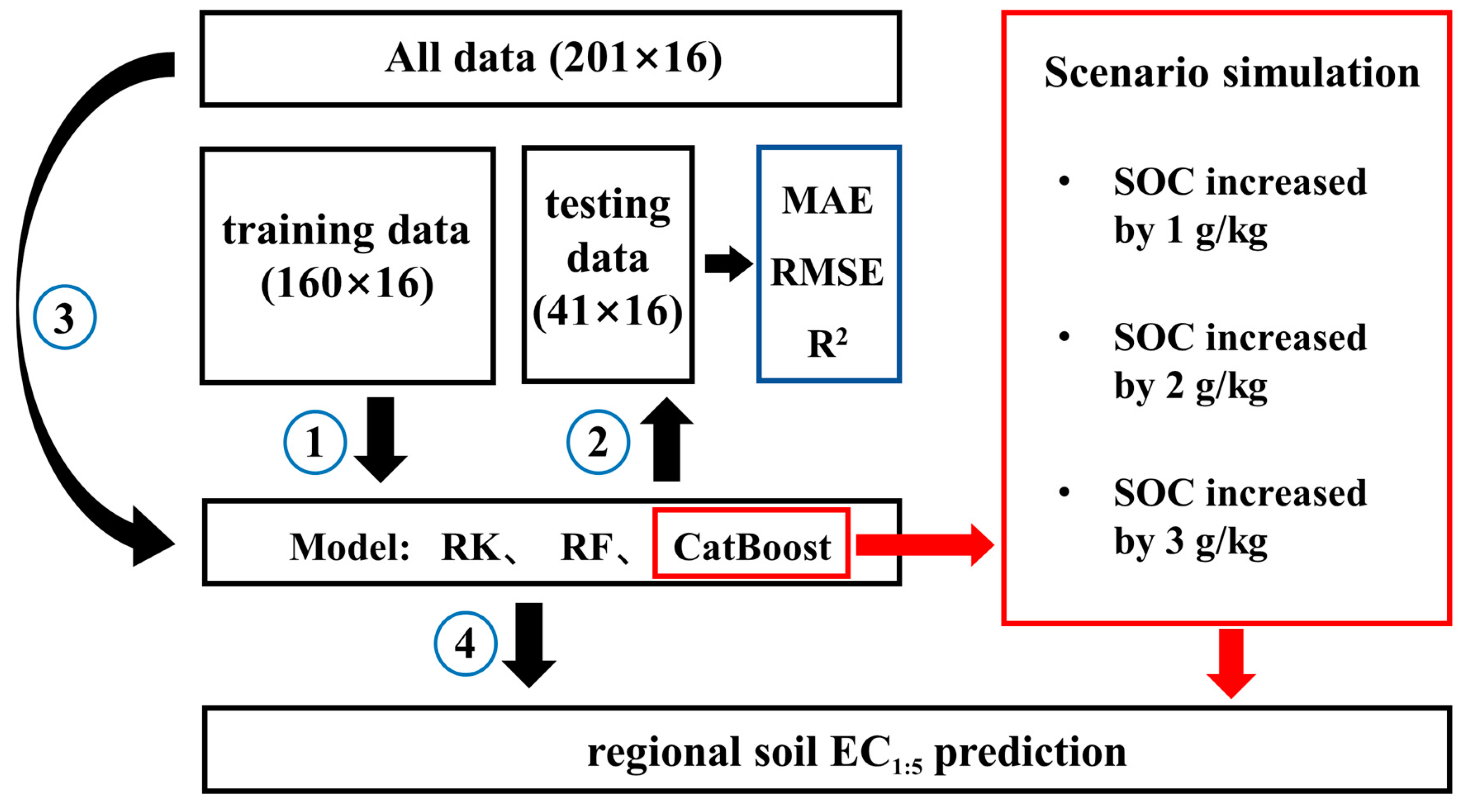
2.4. Spatial Distribution Prediction Methods

2.4.1. EBK Regression

EBK regression prediction is a geostatistical interpolation method that integrates EBK with a known explanatory variable grid to influence the interpolated data values. Unlike traditional Kriging, EBK accounts for the estimation error of the semivariogram model. Its advantage lies in representing local random spatial processes as stationary or non-stationary random fields, where the parameters of the locally defined random field vary spatially [40,41]. EBK regression prediction has been employed to estimate the spatial patterns of target variables in the domains of soil environment, atmospheric environment, and water environment [42,43].
EBK regression prediction was performed using ArcGIS Pro 3.0.1.

2.4.2. Random Forest

The RF algorithm was introduced by Breiman in 2001 as an improvement to bagging and a competitor for boosting [44]. It is widely used for both classification and regression tasks owing to its strong predictive capabilities. Specifically, RF can effectively handle high-dimensional data and multiclass outputs. Furthermore, the model integrates a multitude of tree-based estimators, which collectively outperform a single random tree [45], because each individual tree exhibits low bias but high variance, while an aggregation of trees achieves an optimal balance between bias and variance [46]. Additionally, RF provides measures of variable importance for predicting outcome variables [30].
The RF modeling approach was implemented in R4.2.2 by applying the R package “randomForest”. Two parameters are involved in the establishment of an RF, the number of trees in the classification tree (tree) and the variable selection number (mtry) during branching. This study traversed all mtry values and then determined the mtry value based on minimum mean square error (MSE) values. The tree was set to its default value (tree = 500). Before RF modeling, category variables need to be one-hot encoded.

2.4.3. CatBoost

CatBoost is a powerful machine learning technique for both classification and regression problems. The name, CatBoost, resulted from combining “category” and “boosting”, providing a description of the algorithm in processing category data. It uses an efficient preprocessing method called target-based statistics (TBS) to reduce target leakage [19], thus helping to improve the performance of the algorithm when working with categorical data. CatBoost employs an ordered boosting technique to modify gradient estimation and uses oblivious trees as predictors to prevent overfitting [11]. This algorithm is remarkably faster than many other models in terms of training speed because it can be supported with a graphical processing unit. Additionally, it is robust and requires fewer hyperparameters for tuning [19].
The CatBoost model is run in R4.2.2 by applying the R package “catboost”. The learning rate and number of iterations are the key hyperparameters of the CatBoost model. A learning rate of 0.10 was selected among three options (0.05, 0.10, and 0.15) to minimize the MSE value. In this study, 200 iterations were performed per convention. Moreover, CatBoost can be set to “the best model” parameters.
The “catboost” package can produce values for variable importance and SHapley Additive exPlanations (SHAP). SHAP is an additive interpretation model based on the game theory proposed by Lundberg and Lee, and it can measure the impact of individual variables on machine learning model predictions [47]. Additionally, it reveals the degree of contribution of the different variables to each prediction value. Compared with other interpretation methods, SHAP not only addresses the issue of multicollinearity, but considers possible synergistic effects between variables as well [48].

2.4.4. Model Train and Test

The data were sorted according to the longitude of the sampling points, and 21 sites were randomly selected. This step was taken to ensure an even distribution of sample points within the study area. This process was repeated for point latitude (replacing duplicates manually), resulting in a total of 41 sample data point. By following the above steps, 41 data point (25%) were selected as the test set, with the remaining ones (75%) used as the training set. This process was repeated 10 times to obtain 10 training and test sets. Training data were used to create a regression model, and the testing data were used to validate the performance of the designed models.
Model performance in predicting soil salinity levels was assessed using the root mean square error (RMSE) and mean absolute error (MAE). Model performance was considered superior when both MAE and RMSE were lower [14,30]. These criteria were assessed using the equations below:
M A E = 1 N i = 1 N | E i M i |
M S E = 1 N i = 1 N ( E i M i ) 2  
R M S E = M S E
where E i is the true value, M i is the predicted value, and N is the number of samples.

2.5. Scenario Simulation

To predict the spatial distribution pattern of soil salinity in the Yellow River Delta, three models with optimal neutral performance were utilized. SOC has a good improvement effect on saline soil. The adjusted data, reflecting increases in SOC by 1 g/kg, 2 g/kg, and 3 g/kg, were input into the optimal model to forecast the spatial distribution of soil salinity. The results were visualized using ArcMap.

2.6. Digital Soil Mapping

Digital soil mapping was performed using the ArcMap software (version 10.6). To obtain explanatory variable values for areas other than the sampling points, we used the fishnet tool to divide the study area into 23,205 cells with a resolution of 600 m × 600 m. Each cell was assigned a value through its center point, and these values were then input into the model for prediction. The predicted EC1:5 values were matched to the corresponding grids and visualized. This method produced soil EC1:5 distribution maps with varying accuracies.
The conceptual framework of soil EC1:5 prediction is shown in Figure 2.

3. Results

3.1. Descriptive Statistics of EC1:5

Table 2 shows a statistical description of soil EC1:5. The study area exhibited a wide range of soil EC1:5 values, from a low of 0.03335 ds/m to a high of 22.30 ds/m, with a coefficient of variation (CV) of 157.78%. The median and mean values were 0.6541 and 2.7574 ds/m, respectively, indicating skewed data.

3.2. Pearson Correlation and Variable Importance

The Pearson correlation coefficient and variance inflation factor (VIF) values were calculated in R 4.2.2 (Table 3). The relationship was obtained for the sum of soil sand, clay, and silt contents (a VIF value of 100 for the sum prevented the VIF value for clay from being calculated). Generally, a VIF value greater than 10 indicates strong collinearity in the data. Based on this criterion, clay, sand, and EVP-PRE were removed.
The influencing variables were ranked according to their importance (Figure 3). Among all variables, soil Na showed an absolute advantage in its contribution to soil EC1:5. NDVI was the second most important variable, followed by SOC. Soil EC1:5 was also influenced by pH, DLUC, and coastline1980. Further, among ocean-related variables, coastline1980 had a greater effect on soil EC1:5 than DSWS22. Land-cover types including permanent water bodies, cropland, and build-up area significantly influenced soil EC1:5. Lastly, among all variables, soil type contributed the least.

3.3. Evaluation and Comparison of Model Performance

The results of prediction performance analysis for the four models tested herein are listed in Table S1. The machine learning models outperformed the geostatistical models in terms of prediction performance. The best prediction model in this study was CatBoost, which had the smallest values of MAE (1.86) and RMSE (3.11) and the highest R2 value (0.59). This suggests that the CatBoost model performed well in predicting data containing categorical variables, which is one of its major advantages.

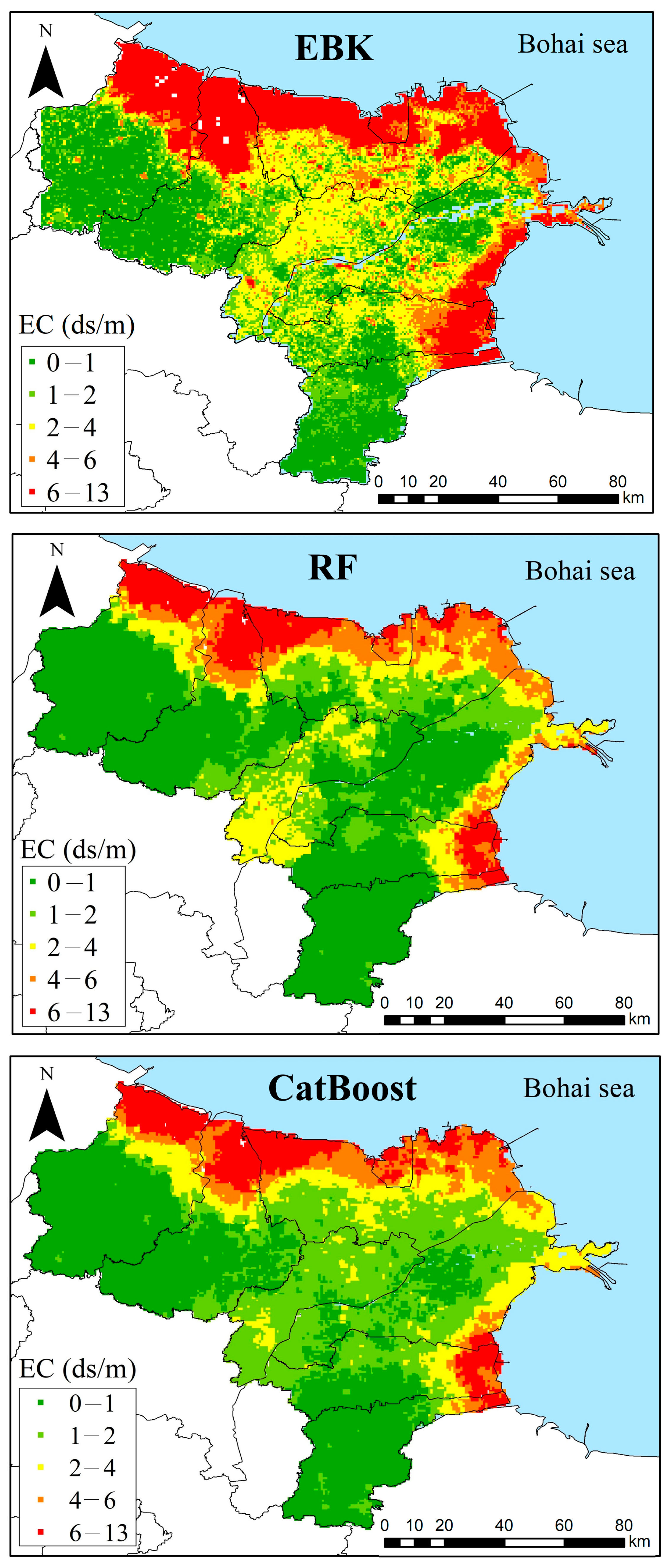
3.4. Mapping Soil Salinity
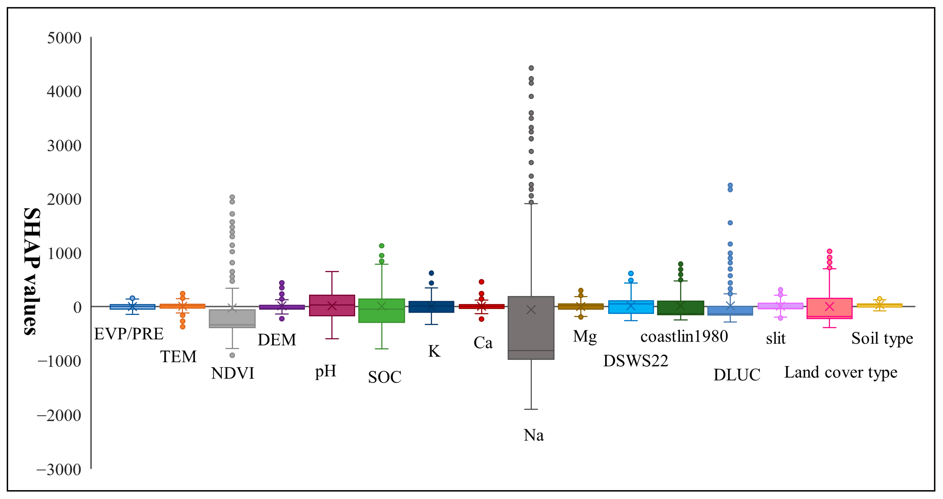
The spatial distributions of soil EC1:5 predicted with the three models are shown in Figure 4. Although all models predicted a higher coastal soil EC1:5, significant differences were observed among them.
Differences in soil salt composition in different regions reportedly lead to differences in the relationship between soil salinity and EC. For coastal areas, the EC1:5 threshold (6‰) for saline soils included but was not limited to 2.0290, 1.9450, 2.0760, and 2.1310 ds/m [5,49,50,51]. Therefore, this study used EC1:5 = 2 ds/m as the minimum value for classifying a soil as saline. The prediction maps produced with the EBK regression models showed that the distribution area of soil EC1:5 values above 2 ds/m was relatively large, accounting for 54.20% of the total surveyed area, respectively. CatBoost predicted that 29.39% of the soil in the study area had an EC1:5 greater than 2 ds/m, whereas RF predicted that the salinity area accounts for 33.82% of the total surveyed area. The prediction results of the four models consistently indicated that the Yellow River Delta region is facing severe soil salinization.

3.5. SHAP Values

In machine-learning algorithms, SHAP values can be used to explain the contribution of each variable to the model. The larger the absolute SHAP value, the greater the importance of the variable [47]. SHAP values calculated for each feature variable under study herein are shown in Figure 5. The SHAP value of Na was the highest, followed by that of NDVI. These findings were consistent with the results on the importance of variables, shown in Figure 3.
To explore the impact of important factors on soil EC1:5, we selected the top six important variables (Na, NDVI, SOC, pH, DLUC, and coastline1980) and two category variables (land cover type and soil type) for an in-depth analysis. The SHAP values for Na and DLUC increased as their respective values increased. In contrast, a downward trend was observed for NDVI, SOC, pH, and coastline1980. When soil Na2O content was above 2.40%, it had a positive effect on the soil EC1:5, such that the higher the Na2O content, the greater the soil EC1:5. As for NDVI, when its value was very low, it had a positive and strong impact on soil EC1:5. Moreover, as the NDVI value increased, its influence on soil EC1:5 decreased, with a value above 0.40 having a negative impact on soil EC1:5. Similarly, as SOC content increased, its influence on soil EC1:5 decreased and changed from positive to negative. Despite Pearson correlation coefficients indicating a weak correlation between pH and soil EC1:5 (−0.07), SHAP values showed that, when the pH was below 8.4, it positively impacted soil EC1:5. Thus, the lower the pH, the greater the impact; however, when the pH exceeded 8.4, the trend was reversed, and higher pH values had a greater negative impact on soil EC1:5. Figure 6e shows that when the DLUC value exceeded 0.5, the positive impact on soil EC1:5 gradually increased. Additionally, the proximity of the coastline in 1980 had a significant positive correlation with soil EC1:5 (Figure 6f). As the distance from the coastline increased, the correlation weakened; when it exceeded 8 km, the correlation became negative.
Among land-cover types, the SHAP values of bare/sparse plants and water bodies were positive, indicating that, in these cases, soil EC1:5 was larger. This is consistent with the actual situation because high soil salinity hinders plant growth and renders the surface bare. In contrast, when vegetation was present, soil EC1:5 values were generally lower. The SHAP values of cinnamon soil, coral sandy soil, and alluvial soils were negative, illustrating that their EC1:5 is generally low, whereas the SHAP values of saline and coastal tidal flat saline soils were positive, indicating that they had higher salinity and EC1:5 values.

3.6. Scenario Simulation

Previous research demonstrated that the implementation of measures, such as incorporating straw into fields, applying organic fertilizers, and utilizing biochar can increase the SOC content of agricultural soils by 1–4 g/kg [26,27,28,29]. Elevating SOC levels can decrease salinization and improve soil quality. To assess the potential and effectiveness of SOC in improving saline–alkali soils, we used the CatBoost model to conduct scenario predictions and derived the distribution of soil EC1:5 values following 1, 2, or 3 g/kg increases in SOC content (Figure 7b–d). The results revealed a significant linear relationship between SOC and soil Na2O content (Figure 8). For each 1 g/kg increase in SOC content, the Na2O content correspondingly decreased by 0.0792%. As a result, when SOC was increased by 1, 2, and 3 g/kg, the proportion of soil EC1:5 greater than 2 ds/m decreased by 2.20%, 4.49%, and 5.68%, respectively, while the proportion of soil EC1:5 values greater than 4 ds/m decreased by 6.65%, 11.44%, and 13.44%, respectively (Table 4). Among these scenarios, the addition of 2 g/kg organic carbon yielded the most favorable outcome in terms of ameliorating soil salinity. For soils with EC1:5 > 2 ds/m, the percent reduction (PR) in the area of saline soil across various grades corresponding to a unitarian increase in SOC for scenarios b, c, and d was 2.20%, 2.25%, and 1.89%, respectively (Table 4). The most effective improvement was observed in scenario c. For soils with EC1:5 > 4 ds/m, the most efficient improvement occurred with a SOC increase of 1 g/kg, which resulted in a 6.65% reduction in the area of high salinity. Furthermore, the salinity-amelioration effect tended to stabilize as SOC content increased.

4. Discussion

The Yangtze, Yellow, and Pearl rivers are the three longest rivers in China. Over hundreds of millions of years, these rivers formed expansive alluvial plains in their respective estuaries, namely the Yangtze, Yellow, and Pearl River deltas. Currently, the Yangtze and Pearl River deltas are the two regions with the most advanced economies and the strongest comprehensive strength in China. In comparison, the Yellow River Delta lags significantly in economic output and population size. Land salinization is the primary limiting factor. Therefore, improving saline–alkali land and realizing efficient agricultural planning are crucial issues that must be resolved to promote high-quality development within the region.
According to the variable importance ranking (Figure 3) and SHAP values (Figure 5), soil Na was the most significant factor affecting soil EC1:5. SHAP values for Na revealed that, after exceeding the threshold (approximately 2.40%), the effect of soil Na on EC1:5 increased (Figure 6a). As an important component of soil salinity, Na+ plays a crucial role in coastal areas. Particularly, in the study area, the effects of Na on soil EC1:5 and its correlations were stronger than those of K, Ca, and Mg. Although K was significantly correlated with EC1:5, it was a less important factor. Conversely, NDVI was strongly correlated with soil EC1:5 and soil salinity, which reflected the effects of soil salinity on plant growth [7]. Typically, areas with lower soil EC1:5 have more vegetation and higher NDVI values, consistent with the results of this study (Figure 6b). Soil pH and SOC affect soil salt distribution. Both Pearson correlation coefficient and SHAP values indicate a negative interaction between EC1:5 and SOC, with high SOC levels preventing soil salinization. The application of organic amendments can stimulate the activity of soil microorganisms, reduce soil EC1:5 values, and improve soil structure [52]. Calculated Pearson correlation coefficients suggested no significant correlation between soil pH and EC1:5. However, the SHAP values indicated that the influence of pH on soil EC1:5 initially decreased and then increased (Figure 6d). Thus, soil pH had a positive effect on EC1:5 under weakly alkaline conditions but had a negative effect under strongly alkaline conditions. Land-use change is another important variable. Coastal areas have undergone significant land-use changes due to the development of marine aquaculture and the establishment of offshore farms, resulting in an extended coastline. Land-use changes interact with soil salinity. Soil salinity affects land-use types, and, in turn, different land activities can alter soil salinity. For example, the introduction of mariculture increases soil salinity, while the application of organic fertilizers reduces soil salinity. Despite the relatively low contribution of TEM to the prediction of soil EC1:5 in this study, it remains a notable factor in light of global climate change. While Pearson coefficient values suggested an insignificant correlation between TEM and soil EC1:5, the SHAP value revealed a shift from a negative to a positive correlation with increasing temperature. Indeed, temperature increases may have resulted in elevated sea levels, seawater-mediated intensification of soil erosion, and increased salinization. Among the two oceanic variables, coastline1980 was relatively important. The ocean acts as a vast salt repository, with the coastline demarcating its boundaries. This effect decreased with increasing distance from the coastline. Although variations in oceanic salinity were observed among the different regions of the Bohai Sea, these differences were not significant for terrestrial soils.
Currently, the prediction of soil salinity in the Yellow River Delta region primarily relies on remote sensing image inversion [7,8,53]. Limited research has combined multi-source environmental data and machine learning models for this purpose. Wang et al. (2024) utilized remote sensing data and machine learning methods to create a soil salinity distribution map of the Yellow River Delta, revealing that severely saline soils account for 43% of the area [53]. The prediction results from our study indicate that approximately one-third to half of the land in the Yellow River Delta is affected by salinization. Moreover, the heavily saline areas are predominantly located in the eastern and northern coastal regions, with surface soil salinity decreasing from coastal to inland areas. This pattern is consistent with findings from other studies on coastal saline soils [8,47,54]. The coastal zone had particularly high EC1:5 values because of its flat terrain, which is susceptible to erosion by seawater (high in sodium chloride content). In addition, the large area of marine aquaculture and salt fields in the region contribute to the continuously high sodium level in the soil. The CatBoost model demonstrated the greatest predictive efficacy. Its ability to handle categorical data is a key advantage, as confirmed in this study. In a comparative analysis conducted by Mantena et al., 2023, the CatBoost model surpassed the XGBoost and LightGBM models in terms of precision in predicting soil salinity [55]. In a study by Lu et al., (2023), CatBoost outperformed RF in predicting soil pH based on its higher accuracy and better fitting effects [11]. Similarly, when predicting groundwater salinity, CatBoost showed the best neutral performance and the highest prediction accuracy compared with the RF, XGBoost, and LightGBM models [19]. By integrating multi-source data with CatBoost’s robust regression prediction capabilities, data processing efficiency can be enhanced, complex nonlinear relationships can be captured, and the accuracy of soil salinity predictions can be improved.
To amend or alleviate the serious issue of soil salinization in the Yellow River Delta region, organic improvement materials such as biochar have been used to enhance the quality of saline–alkali land [24,56]. Consistent with this generalization, studies have shown that straw return mitigates soil salinization by increasing SOC content. In this study, three SOC improvement scenarios were evaluated, the results of which indicated that increasing SOC content by 1 g/kg yielded the best improvement effect on saline alkali soil with EC1:5 > 4 ds/m, while increasing the SOC content by 2 g/kg had the best effect on soils with EC1:5 > 2 ds/m. Lastly, to improve soil with EC1:5 > 4 ds/m, the optimal approach is to increase SOC by 1 g/kg. For further improvement of land with EC1:5 > 2 ds/m, scenario c (increase in SOC by 2 g/kg) demonstrated the most effective improvement. Additionally, the remediation of saline–alkali land does not simply involve increasing the quantity of organic amendments. Instead, it is important to comprehensively consider economic costs and environmental benefits and select an application dose that is both effective and cost-efficient.
There are several uncertainties in this research. First, despite the availability of 200 samples, the Kriging interpolation distribution maps (sodium, potassium, calcium, magnesium, pH, and SOC) derived from these samples inherently contain uncertainty. Second, although there is a significant linear correlation between sodium and organic carbon in the Yellow River Delta region, the actual relationship between the addition of organic carbon and the reduction in sodium content may not strictly follow this linear correlation, introducing additional uncertainty.
This research took into consideration the unique environmental influence of the ocean and used the SHAP model to conduct an in-depth exploration of the key factors influencing soil salinity. The CatBoost model was used to estimate soil EC1:5 in the Yellow River Delta, and distribution maps of soil EC1:5 at various levels were subsequently generated. This process effectively substantiated the robust predictive capabilities of the CatBoost model. Furthermore, this study identified the most effective strategy for enhancing SOC in saline–alkali soils through predictive modeling under a range of scenarios. These findings offer valuable insights that should be instrumental in governmental decision-making processes regarding agricultural development planning.
However, this study is not without limitations. First, the sample size was somewhat restricted due to the extensive coastal aquaculture areas and the presence of the Yellow River Delta Nature Reserve. Additionally, this study employed only two machine learning models for prediction; future research could explore a wider range of machine learning methods to enhance predictive accuracy. Finally, this study did not incorporate household surveys, thus limiting the exploration of potential impacts from additional socio-economic factors. These areas present opportunities for further research and refinement in future studies.

5. Conclusions

This study used the CatBoost model to predict soil salt content and plot a salinity-areas distribution map. Simultaneously, it improved upon previously used methods by measuring soil properties related to soil salinity (e.g., K, Ca, Na, Mg, SOC, and pH) in the laboratory and considering the impact of the ocean on coastal soil. Moreover, important factors affecting soil salinity were comprehensively explored using the SHAP model. The results indicated that (1) CatBoost showed the highest accuracy (MAE = 1.86, RMSE = 3.11, R2 = 0.59) compared to the other three models, thus confirming its excellent prediction potential; (2) both variable importance ranking and SHAP values indicated that soil Na and NDVI were the two most important factors affecting EC. In addition, soil pH, SOC, and DLUC significantly affected soil EC1:5; (3) soil salinization is a serious issue in the Yellow River Delta region, especially in the coastal zones due to seawater erosion and human activities; (4) increasing SOC by 1 g/kg yielded the best improvement effect on soils with EC1:5 > 4 ds/m, while increasing SOC by 2 g/kg yielded the best improvement effect on soils with EC1:5 > 2 ds/m. Based on the spatial distribution characteristics of soil salinity, targeted improvement of soils with varying degrees of salinization, which is the ultimate goal of this study, can be conducted. This study provided useful insights for the precise spatial prediction of soil salinity and efficient improvement of coastal saline–alkali soils.

Supplementary Materials

The following supporting information can be downloaded at: https://www.mdpi.com/article/10.3390/rs16142681/s1, Figure S1: The laboratory determination of soil indicators. a: pH; b: SOC; c: K2O; d: CaO; e: Na2O; f: MgO; Figure S2. The explanatory variables. a: evaporation; b: precipitation; c: NDVI; d: DEM; e: DSWS22; f: coastline1980; g: DLUC; h: land cover type; i: slit content; j: soil type; Table S1: The prediction accuracy of different methods.

Author Contributions

M.Z.: Methodology, Data collection, Software, Validation, Writing—original draft, Writing—review and editing, Visualization. Y.L.: Conceptualization, Supervision, Writing—review and editing, Funding acquisition. All authors have read and agreed to the published version of the manuscript.

Funding

This work was supported by the Strategic Priority Research Program of the Chinese Academy of Sciences (Grant No. XDA26050202).

Data Availability Statement

The data presented in this study are available on request from the corresponding author and with permission of the Institute of Geographic Sciences and Natural Resources Research, Chinese Academy of Sciences. The data are not publicly available due to confidentiality requirements.

Conflicts of Interest

The authors declare that they have no known competing financial interests or personal relationships that could have appeared to influence the work reported in this paper.

References

  1. Chen, J.; Mueller, V. Coastal climate change, soil salinity and human migration in Bangladesh. Nat. Clim. Change 2018, 8, 981–985. [Google Scholar] [CrossRef]
  2. Singh, A. Soil salinization management for sustainable development: A review. J. Environ. Manag. 2021, 277, 111383. [Google Scholar] [CrossRef]
  3. Food and Agriculture Organization of the United Nations (FAO). World Map of Salt-Affected Soils Launched at Virtual Conference. 2021. Available online: https://www.fao.org/newsroom/detail/salt-affected-soils-map-symposium/en (accessed on 7 March 2023).
  4. Hassan, A.; Azapagic, A.; Shokri, N. Global predictions of primary soil salinization under changing climate in the 21st century. Nat. Commun. 2021, 12, 6663. [Google Scholar] [CrossRef] [PubMed]
  5. Yao, R.J.; Yang, J.S.; Zhou, P.; Zhou, P. Spatial variability of soil salinity in characteristic field of the Yellow River Delta. Trans. Chin. Soc. Agric. Eng. 2006, 22, 61–66. [Google Scholar]
  6. Mohammadifar, A.; Gholami, H.; Golzar, S. Assessment of the uncertainty and interpretability of deep learning models for mapping soil salinity using DeepQuantreg and game theory. Sci. Rep. 2022, 12, 15167. [Google Scholar] [CrossRef] [PubMed]
  7. Guo, B.; Yang, X.; Yang, M.; Sun, D.; Zhu, W.; Zhu, D.; Wang, J. Mapping soil salinity using a combination of vegetation index time series and single-temporal remote sensing images in the Yellow River Delta, China. Catena 2023, 231, 107313. [Google Scholar] [CrossRef]
  8. Li, Y.; Chang, C.; Wang, Z.; Zhao, G. Upscaling remote sensing inversion and dynamic monitoring of soil salinization in the Yellow River Delta, China. Ecol. Indic. 2023, 148, 110087. [Google Scholar] [CrossRef]
  9. Jiang, H.; Shu, H. Optical remote-sensing data based research on detecting soil salinity at different depth in an arid-area oasis, Xinjiang, China. Earth Sci. Inform. 2019, 12, 43–56. [Google Scholar] [CrossRef]
  10. Guo, B.; Yang, F.; Fan, Y.; Han, B.; Chen, S.; Yang, W. Dynamic monitoring of soil salinization in Yellow River Delta utilizing MSAVI–SI feature space models with Landsat images. Environ. Earth Sci. 2019, 78, 308. [Google Scholar] [CrossRef]
  11. Lu, Q.K.; Tian, S.; Wei, L.F. Digital mapping of soil pH and carbonates at the European scale using environmental variables and machine learning. Sci. Total Environ. 2023, 856, 159171. [Google Scholar] [CrossRef]
  12. Zhang, H.; Yin, S.H.; Chen, Y.H.; Shao, S.S.; Wu, J.T.; Fan, M.M.; Chen, F.R.; Gao, H. Machine learning-based source identification and spatial prediction of heavy metals in soil in a rapid urbanization area, eastern China. J. Clean. Prod. 2020, 273, 122858. [Google Scholar] [CrossRef]
  13. Nguyen, T.T.; Ngo, H.H.; Guo, W.; Chang, S.W.; Nguyen, D.D.; Nguyen, C.T.; Zhang, J.; Liang, S.; Bui, X.T.; Hoang, N.B. A low-cost approach for soil moisture prediction using multi-sensor data and machine learning algorithm. Sci. Total Environ. 2022, 833, 155066. [Google Scholar] [CrossRef] [PubMed]
  14. Agyeman, P.C.; Kingsley, J.; Kebonye, N.M.; Khosravi, V.; Borůvka, L.; Vašát, R. Prediction of the concentration of antimony in agricultural soil using data fusion, terrain attributes combined with regression kriging. Environ. Pollut. 2023, 316, 120697. [Google Scholar] [CrossRef] [PubMed]
  15. Guo, Y.; Yang, Y.; Li, R.; Liao, X.; Li, Y. Cadmium accumulation in tropical island paddy soils: From environment and health risk assessment to model prediction. J. Hazar. Mater. 2024, 465, 133212. [Google Scholar] [CrossRef] [PubMed]
  16. Ngu, N.H.; Thanh, N.N.; Duc, T.T.; Non, D.Q.; An, N.T.T.; Chotpantarat, S. Active learning-based random forest algorithm used for soil texture classification mapping in Central Vietnam. Catena 2024, 234, 107629. [Google Scholar] [CrossRef]
  17. Siqueira, R.G.; Moquedace, C.M.; Fernandes-Filho, E.I.; Schaefer, C.E.G.R.; Francelino, M.R.; Sacramento, I.F.; Michel, R.F.M. Modelling and prediction of major soil chemical properties with Random Forest: Machine learning as tool to understand soil-environment relationships in Antarctica. Catena 2024, 235, 107677. [Google Scholar] [CrossRef]
  18. Pham, T.D.; Yokoya, N.; Nguyen, T.T.T.; Le, N.N.; Ha, N.T.; Xia, J.; Takeuchi, W.; Pham, T.D. Improvement of Mangrove Soil Carbon Stocks Estimation in North Vietnam Using Sentinel-2 Data and Machine Learning Approach. GISci. Remote Sens. 2021, 58, 68–87. [Google Scholar] [CrossRef]
  19. Tran, D.A.; Tsujimura, M.; Ha, N.T.; Nguyen, V.T.; Binh, D.V.; Dang, T.D.; Doan, Q.; Bui, D.T.; Ngoc, T.A.; Phu, L.V.; et al. Evaluating the predictive power of different machine learning algorithms for groundwater salinity prediction of multi-layer coastal aquifers in the Mekong Delta, Vietnam. Ecol. Indic. 2021, 127, 107790. [Google Scholar] [CrossRef]
  20. Huang, G.A.; Wu, L.F.; Ma, X.; Zhang, W.; Fan, J.; Yu, X.; Zeng, W.; Zhou, H. Evaluation of CatBoost method for prediction of reference evapotranspiration in humid regions. J. Hydrol. 2019, 574, 1029–1041. [Google Scholar] [CrossRef]
  21. Jabeur, S.B.; Gharib, C.; Mefteh-Wali, S.; Arf, W.B. CatBoost model and artificial intelligence techniques for corporate failure prediction. Technol. Forecast. Soc. Chang. 2021, 166, 120658. [Google Scholar] [CrossRef]
  22. Xiang, W.; Xu, P.; Fang, J.; Zhao, Q.; Gu, Z.; Zhang, Q. Multi-dimensional data-based medium- and long-term power-load forecasting using double-layer CatBoost. Energy Rep. 2022, 8, 8511–8522. [Google Scholar] [CrossRef]
  23. Wei, X.; Rao, C.; Xiao, X.; Chen, L.; Goh, M. Risk assessment of cardiovascular disease based on SOLSSA-CatBoost model. Expert Syst. Appl. 2023, 219, 119648. [Google Scholar] [CrossRef]
  24. Ouyang, Z.; Wang, H.; Lai, J.; Wang, C.; Liu, Z.; Sun, Z.; Hou, R. New Approach of High-quality Agricultural Development in the Yellow River Delta. Bull. Chin. Acad. Sci. 2020, 35, 145–153. [Google Scholar] [CrossRef]
  25. Li, G. A Summary on Soil Salinization of Yellow River Delta. Anhui Agri. Sci. Bull. 2020, 26, 02–03. [Google Scholar] [CrossRef]
  26. Tian, S.Z.; Ning, T.Y.; Wang, Y.; Li, H.; Zhong, W.; Li, Z. Effect of different tillage methods and straw-returning on soil organic carbon content in a winter wheat field. Chin. J. Appl. Ecol. 2010, 21, 373–378. [Google Scholar] [CrossRef]
  27. Xu, G.X.; Wang, Z.F.; Gao, M.; Tian, D.; Huang, R.; Liu, J.; Li, J.C. Effects of straw and biochar return on soil aggregate and carbon sequestration. Chin. J. Environ. Sci. 2018, 39, 355–362. [Google Scholar] [CrossRef]
  28. Guo, K.; He, G.; Wang, C.; Zhang, H.; Yan, X.; Wang, S.; Kong, Y.; Zhou, G.; Hu, R. Biochar amendment ameliorates soil properties and promotes Miscanthus growth in a coastal saline-alkali soil. Appl. Soil Ecol. 2020, 155, 103674. [Google Scholar] [CrossRef]
  29. Crystal-Ornelas, R.; Thapa, R.; Tully, K.L. Soil organic carbon is affected by organic amendments, conservation tillage, and cover cropping in organic farming systems: A meta-analysis. Agric. Ecosyst. Environ. 2021, 312, 107356. [Google Scholar] [CrossRef]
  30. Zhou, M.; Li, Y. Spatial distribution and source identification of potentially toxic elements in Yellow River Delta soils, China: An interpretable machine-learning approach. Sci. Total Environ. 2024, 912, 169092. [Google Scholar] [CrossRef]
  31. Ning, Z.; Li, D.; Chen, C.; Xie, C.; Chen, G.; Xie, T.; Wang, Q.; Bai, J.; Cui, B. The importance of structural and functional characteristics of tidal channels to smooth cordgrass invasion in the Yellow River Delta, China: Implications for coastal wetland management. J. Environ. Manag. 2023, 342, 118297. [Google Scholar] [CrossRef]
  32. Ministry of Natural Resources of the People’s Republic of China. Soil Determination of pH—Potentiometry (HJ 962-2018). 2019. Available online: https://www.mee.gov.cn/ywgz/fgbz/bz/bzwb/jcffbz/201808/t20180815_451430.shtml (accessed on 13 April 2023).
  33. GBW07986; Certified Reference Material for the Chemical Composition of Soil. Institute of Geophysical and Geochemical Exploration: Langfang, China, 2021.
  34. Xu, X.L. China Annual Vegetation Index (NDVI) Spatial Distribution Dataset. Resource and Environmental Science Data Registration and Publishing System (RESDRPS). 2018. Available online: https://www.resdc.cn/DOI/doi.aspx?DOIid=49 (accessed on 6 March 2023). [CrossRef]
  35. Xu, X.L.; Liu, J.Y.; Zhang, S.W.; Li, R.; Yan, C.; Wu, S. Multi period Land Use Remote Sensing Monitoring Dataset in China. RESDRPS. 2018. Available online: https://www.resdc.cn/DOI/doi.aspx?DOIid=54 (accessed on 6 March 2023). [CrossRef]
  36. Xu, X.L. Annual Spatial Interpolation Dataset of Meteorological Elements in China. RESDRPS. 2022. Available online: https://www.resdc.cn/DOI/doi.aspx?DOIid=96 (accessed on 7 March 2023). [CrossRef]
  37. Ministry of Ecology and Environment of the People’s Republic of China, National Catalogue Service for Geographic Information. 1:1 Million Basic Geographic Information Data. 2021. Available online: https://www.webmap.cn/main.do?method=index (accessed on 6 March 2023).
  38. Copernicus Marine Service (CMS). Global Ocean 1/12° Physics Analysis and Forecast Updated Daily. 2023. Available online: https://data.marine.copernicus.eu/product/GLOBAL_ANALYSISFORECAST_PHY_001_024/description (accessed on 9 March 2023).
  39. Zanaga, D.; Van De Kerchove, R.; De Keersmaecker, W.; Souverijns, N.; Brockmann, C.; Quast, R.; Wevers, J.; Grosu, A.; Paccini, A.; Vergnaud, S.; et al. ESA WorldCover 10 m 2020 v100 (Version v100) [Data Set]. Zenodo. 2021. Available online: https://worldcover2020.esa.int/download (accessed on 8 March 2023).
  40. Zhang, F.; Li, X.; Zhou, X.; Chan, N.W.; Tan, M.L.; Kung, H.T.; Shi, J. Retrieval of soil salinity based on multi-source remote sensing data and differential transformation technology. Int. J. Remote Sens. 2023, 44, 1348–1368. [Google Scholar] [CrossRef]
  41. Zhang, B.; Hou, H.; Liu, L.; Huang, Z.; Zhao, L. Spatial prediction and influencing factors identification of potential toxic element contamination in soil of different karst landform regions using integration model. Chemosphere 2023, 327, 138404. [Google Scholar] [CrossRef] [PubMed]
  42. Senoro, D.B.; de Jesus, K.L.M.; Mendoza, L.C.; Apostol, E.M.D.; Escalona, K.S.; Chan, E.B. Groundwater Quality Monitoring Using In-Situ Measurements and Hybrid Machine Learning with Empirical Bayesian Kriging Interpolation Method. Appl. Sci. 2022, 12, 132. [Google Scholar] [CrossRef]
  43. Aldegunde, J.A.Á.; Sánchez, A.F.; Saba, M.; Bolaños, E.Q.; Palenque, J.Ú. Analysis of PM2.5 and Meteorological Variables Using Enhanced Geospatial Techniques in Developing Countries: A Case Study of Cartagena de Indias City (Colombia). Atmosphere 2022, 13, 506. [Google Scholar] [CrossRef]
  44. Cutler, A.; Cutler, D.R.; Stevens, J.R. Random Forests. In Ensemble Machine Learning; Zhang, C., Ma, Y., Eds.; Springer: New York, NY, USA, 2012. [Google Scholar] [CrossRef]
  45. Cao, J.; Guo, Z.H.; Ran, H.Z.; Xu, R.; Anaman, R.; Liang, H.Z. Risk source identification and diffusion trends of metal(loid)s in stream sediments from an abandoned arsenic-containing mine. Environ. Pollut. 2023, 329, 121713. [Google Scholar] [CrossRef] [PubMed]
  46. Zhen, Y.; Wang, L.; Sun, H.; Liu, C. Prediction of microplastic abundance in surface water of the ocean and influencing factors based on ensemble learning. Environ. Pollut. 2023, 331, 121834. [Google Scholar] [CrossRef] [PubMed]
  47. Lundberg, S.M.; Lee, S.I. A unified approach to interpreting model predictions. In Proceedings of the 31st International Conference on Neural Information Processing Systems, Long Beach, CA, USA, 4–9 December 2017; Volume 30, pp. 4768–4777. [Google Scholar]
  48. Lundberg, S.M.; Erion, G.; Chen, H.; DeGrave, A.; Prutkin, J.M.; Nair, B.; Katz, R.; Himmelfarb, J.; Bansal, N.; Lee, S. From local explanations to global understanding with explainable AI for trees. Nat. Mach. Intell. 2020, 2, 56–67. [Google Scholar] [CrossRef] [PubMed]
  49. Yao, R.J.; Yang, J.S.; Zou, P.; Liu, G.; Yu, S. Quantitative Evaluation of the Field Soil Salinity and Its Spatial Distribution Based on Electromagnetic Induction Instruments. Sci. Agric. Sin. 2008, 41, 460–469. [Google Scholar] [CrossRef]
  50. Wang, Y.; Wang, Z.; Lian, X.; Xiao, H.; Wang, L.; He, H. Measurement of Soil Electric Conductivity and Relationship Between Soluble Salt Content and Electrical Conductivity in Tianjin Coastal Area. Tianjin Agric. Sci. 2011, 17, 18–21. [Google Scholar] [CrossRef]
  51. Li, R.; Wang, F.; Qin, F.; Lou, F.; Wu, D. Studies on the Best Curve Equation Between the Total Salts and the Electrical Conductivity of the Coastal Saline Soil. J. Agric. 2015, 25, 59–62. [Google Scholar] [CrossRef]
  52. Rao, D.L.N.; Pathak, H. Ameliorative influence of organic matter on biological activity of salt-affected soils. Arid. Soil Res. Rehab. 1996, 10, 311–319. [Google Scholar] [CrossRef]
  53. Fan, X.; Weng, Y.; Tao, J. Towards decadal soil salinity mapping using Landsat time series data. Int. J. Appl. Earth Obs. Geoinf. 2016, 52, 32–41. [Google Scholar] [CrossRef]
  54. Wang, J.; Wang, X.; Zhang, J.; Shang, X.; Chen, Y.; Feng, Y.; Tian, B. Soil Salinity Inversion in Yellow River Delta by Regularized Extreme Learning Machine Based on ICOA. Remote Sens. 2024, 16, 1565. [Google Scholar] [CrossRef]
  55. Mantena, S.; Mahammood, V.; Rao, K.N. Prediction of soil salinity in the Upputeru river estuary catchment, India, using machine learning techniques. Environ. Monit. Assess. 2023, 195, 1006. [Google Scholar] [CrossRef] [PubMed]
  56. Manasa, M.R.K.; Katukuri, N.R.; Nair, S.S.D.; Haojie, Y.; Yang, Z.; Guo, R. Role of biochar and organic substrates in enhancing the functional characteristics and microbial community in a saline soil. J. Environ. Manag. 2020, 269, 110737. [Google Scholar] [CrossRef]
Figure 1. Map of the study area and sampling sites.
Remotesensing 16 02681 g001
Figure 2. The framework of soil EC1:5 prediction.
Remotesensing 16 02681 g002
Figure 3. Importance of variables: Red represents CatBoost (a) and blue represents RF (b).
Remotesensing 16 02681 g003
Figure 4. Spatial prediction maps of soil EC1:5.
Remotesensing 16 02681 g004
Figure 5. The box plot of SHAP values of all characteristic variables. The points are outliers.
Remotesensing 16 02681 g005
Figure 6. The SHAP values of Na (a), NDVI (b), SOC (c), pH (d), DLUC (e), coastline1980 (f), land-cover type (g), and soil type (h). A high |SHAP| value indicates a significant impact. SHAP value > 0: positive impact; SHAP value < 0: negative impact.
Remotesensing 16 02681 g006
Figure 7. Scenario prediction of soil EC1:5. (a) current situation; (b) 1 g/kg SOC increase; (c) 2 g/kg SOC increase; and (d) 3 g/kg SOC increase.
Remotesensing 16 02681 g007
Figure 8. The relationship between SOC and soil Na2O. The dashed line in the figure represents the regression line between SOC and Na2O.
Remotesensing 16 02681 g008
Table 1. Data used for soil salinity prediction modeling.
DataVariablesDescription
Meteorological dataEvaporation (EVP)A 1 km grid based on daily observation data of meteorological element stations from more than 2400 stations in China in 2020. The spatial resolution of this variable is 1 × 1 km.
Precipitation (PRE)
Temperature (TEM)
Remote dataNDVIA 1 km grid based on SPOT/VEGETATION PROBA-V 300 M PRODUCTS vegetation index data. The spatial resolution of this variable is 1 × 1 km.
DEMSRTMDEMUTM 90 M resolution digital elevation data product. The spatial resolution of this variable is 90 × 90 m.
Sea dataDistance to seawater salinity line (DSWS22)Seawater salinity grid map for June 2020 with a spatial resolution of 0.083° × 0.083°. Distance to where the seawater salinity is 22 g/kg. The spatial resolution of this variable is 10 × 10 km.
Coastline 1980The 1980 coastline was derived from a land use dataset created through manual visual interpretation, utilizing Landsat remote sensing images from the United States as the primary source of information. The data feature the European distance from the sampling point to the 1980 coastline. The spatial resolution of this variable is 600 × 600 m.
Environmental dataLand cover typeThe ESA WorldCover 10 m 2020 product provides a global land cover map for 2020 at 10 m resolution based on Sentinel-1 and Sentinel-2 data. The spatial resolution of this variable is 10 × 10 m.
Degree of land use change (DLUC)A 1 km grid based on Landsat remote sensing images. The spatial resolution of this variable is 600 × 600 m.
Soil typeIt is digitally generated according to the “1:1 million Soil Map of the People’s Republic of China” compiled and published by the National Soil Census Office in 1995. The spatial resolution of this variable is 1 × 1 km.
Soil dataSand contentThe spatial distribution data of soil texture in China is compiled based on the 1:1 million soil type map and the soil profile data obtained from the second soil census. The spatial resolution of this variable is 600 × 600 m.
Clay content
Silt content
EC, pH, SOC, K, Ca, Na, and MgMeasured in the laboratory.
Table 2. Statistical description of EC1:5.
EC1:5 (us/cm)NumberMin.MedianMeanMax.SDCV%
0–11180.03330.20290.30900.99900.249880.84
1–2161.06101.77181.57001.99350.353522.52%
2–4182.09502.91972.81513.67200.536619.06%
4–6174.09254.89004.98205.90000.571311.47%
>6326.05009.780011.165422.30004.717942.25%
Total2010.03340.65412.757422.30004.3507157.78
Table 3. VIF and Pearson correlation between soil EC1:5 and other variables.
FactorsPearson CorrelationVIF1VIF2FactorsPearson CorrelationVIF1VIF2
pH−0.071.351.34EVP-PRE−0.19132.77\
SOC−0.42 **2.112.10EVP/PRE−0.16 *98.694.90
K−0.24 **2.052.04coastline1980−0.39 **7.246.05
Ca−0.052.352.32DSWS22−0.44 **8.735.83
Na0.53 **1.931.93Clay−0.30 **\\
Mg−0.012.812.80Slit−0.34 **129.031.48
NDVI−0.62 **2.972.71Sand−0.32 **131.55\
DEM−0.36 **3.113.08DLUC0.50 **2.912.91
TEM0.1013.075.26
*: p < 0.05; **: p < 0.01. VIF1: for all variables; VIF2: variables with strong collinearity were eliminated.
Table 4. Prediction of soil EC1:5 proportion under different SOC application scenarios based on the CatBoost model.
abcd
ProportionProportionPRProportionPRProportionPR
>2 ds/m29.39%27.19%2.20%24.90%2.25%23.71%1.89%
>4 ds/m18.10%11.45%6.65%6.66%5.72%4.66%4.48%
>6 ds/m9.46%3.91%5.55%1.32%4.07%0.23%3.08%
PR: The percent reduction in the area of saline soils across various grades corresponding to each unitarian increase in SOC content.
Disclaimer/Publisher’s Note: The statements, opinions and data contained in all publications are solely those of the individual author(s) and contributor(s) and not of MDPI and/or the editor(s). MDPI and/or the editor(s) disclaim responsibility for any injury to people or property resulting from any ideas, methods, instructions or products referred to in the content.

