Abstract
Continuous and dense time series of satellite remote sensing data are needed for several land monitoring applications, including vegetation phenology, in-season crop assessments, and improving land use and land cover classification. Supporting such applications at medium to high spatial resolution may be challenging with a single optical satellite sensor, as the frequency of good-quality observations can be low. To optimize good-quality data availability, some studies propose harmonized databases. This work aims at developing an ‘all-in-one’ Google Earth Engine (GEE) web-based workflow to produce harmonized surface reflectance data from Landsat-7 (L7) ETM+, Landsat-8 (L8) OLI, and Sentinel-2 (S2) MSI top of atmosphere (TOA) reflectance data. Six major processing steps to generate a new source of near-daily Harmonized Landsat and Sentinel (HLS) reflectance observations at 30 m spatial resolution are proposed and described: band adjustment, atmospheric correction, cloud and cloud shadow masking, view and illumination angle adjustment, co-registration, and reprojection and resampling. The HLS is applied to six equivalent spectral bands, resulting in a surface nadir BRDF-adjusted reflectance (NBAR) time series gridded to a common pixel resolution, map projection, and spatial extent. The spectrally corresponding bands and derived Normalized Difference Vegetation Index (NDVI) were compared, and their sensor differences were quantified by regression analyses. Examples of HLS time series are presented for two potential applications: agricultural and forest phenology. The HLS product is also validated against ground measurements of NDVI, achieving very similar temporal trajectories and magnitude of values (R2 = 0.98). The workflow and script presented in this work may be useful for the scientific community aiming at taking advantage of multi-sensor harmonized time series of optical data.
1. Introduction
Continuous and dense time series of satellite remote sensing data are needed for several land monitoring applications, including vegetation phenology [1], fast crop cycles [2], and improving land use and land cover classification [3]. Supporting such applications at medium to high spatial resolution may be challenging with a single optical satellite sensor, as the frequency of good-quality observations usually is low [4]. With the increasing number of Earth observation satellites providing free imagery archives at medium spatial resolution, combining multiple satellite observations into a single dataset can significantly enhance temporal resolutions, improving our ability to detect fine-grained, subtle landscape change patterns across large areas. This, in turn, has become feasible due to advances in affordable data storage and the increased availability of cloud computing structures, such as the NASA Earth Exchange computing facility [5], Google Earth Engine (e.g., [6]), and specialized data cubes software (e.g., [7]).
Landsat and Sentinel-2 data represent the most widely accessible 10–30 m multi-spectral satellite measurements [8]. In combination, data from the currently operational Landsat-7 ETM+, Landsat-8 OLI, and Sentinel-2 MSI can provide global observations with a better than 3-day revisit [9,10]. This potential for synergistic use is due to their similarities in terms of spectral, spatial, and angular characteristics [5,10,11,12,13]. In fact, the spectral and spatial configurations of the S2 MSI sensors were designed to correspond to analogous bands in the Landsat (and SPOT) series of sensors [14]. Nevertheless, there are also a number of differences between these sensor data that should be addressed before the data can be reliably used together [10,11]. Through a process called harmonization, these differences can be mitigated to generate time series data as though they came from a single sensor or from a virtual constellation [15]. Zhang et al. [10] describe harmonization as the process of transforming the data from one sensor so that they are more similar to the other sensor’s data.
Significant and continuous efforts have been made to develop methodologies for the harmonization of Landsat and Sentinel-2 data [5] as well as commercial sensors like the PlanetScope constellation [16]. The NASA Harmonized Landsat and Sentinel (HLS) product integrates L8 OLI and S2 MSI data to deliver a consistent dataset of surface reflectance at a 30 m scale, with a temporal frequency of 2–4 days [5], and PlanetScope tries to match Sentinel MSI data. The harmonization workflow includes atmospheric correction, cloud/shadow masking, geometric resampling, spatial co-registration, corrections for bandpass difference, and bidirectional reflectance distribution function (BRDF) effects [5]. Although the NASA HLS product can be used with confidence in some parts of the world (e.g., in North America [17]), “HLS is still a research product” [18], and the global coverage HLS product (version 2 at the time of writing) still needs better understanding as some technical challenges remain [19], including improving validation and sorting the ‘known issues’ (~20 reported at the time of writing [20,21]). Another challenge is the requirement to download the harmonized data, which can become increasingly difficult with larger volumes, potentially limiting its widespread use. There is an ongoing effort to alleviate this issue by integrating HLS into the GEE catalogue. However, currently, GEE offers only the Landsat component (HLSL30) (the sentinel component HLSS30 is produced separately), meaning that NASA HLS is not fully operational within GEE. Also, NASA HLS does not harmonize Landsat 7 data, which may be important to increase a series density of cloud-free satellite observations, especially prior to the launch of Sentinel 2 B in 2016.
Working on the same baseline principles as the NASA HLS initiative, a few other projects have been advancing the Landsat and Sentinel-2 data integration mainly through developing new tools. Frantz [7] developed the FORCE (Framework for Operational Radiometric Correction for Environmental Monitoring), a freely available software that can produce harmonized Level-2 (and beyond) analysis ready data (ARD) from Landsat and Sentinel-2 archives; a challenge to use this software may be handling the considerable data volume that can be generated (e.g., downloading and storing input images, saving outputs to disc). The “sen2like” tool, proposed by ESA, has been designed to produce L8 and S2 harmonized Level-2 surface reflectance data at 10 m of resolution, primarily aiming at improving agricultural monitoring capabilities [22]; Sen2like is currently in a pre-operational phase [23]. Nguyen et. al [24] proposed a stream processing for the generation of harmonized L7, L8, and S2 at 30 m spatial resolution but using mostly the Google Earth Engine (GEE) cloud platform and its built-in functions; however, unlike our study, the atmospheric correction is conducted outside the GEE web-based code editor, demanding the installation of software and storing of the corrected data, which can be prohibitive with large datasets.
Overall, these initiatives aim at turning Earth Observation (EO) data consistently and systematically into valuable information layers, which is an ongoing challenge for the EO community [25] with the ever-increasing number of available EO data.
Emphasizing web-based processing instead of download-driven approaches is a current trend and challenge in the field of big EO data [25]. Google Earth Engine (GEE) has become a popular cloud-based platform solution, offering a web-based integrated programming environment and an API for pixel-based image processing, enabling local-to-planetary scale studies without the need for extensive data management or in-house high-performance computing infrastructure [26]. In GEE, the most common archives of remote sensing data (e.g., Landsat and Sentinel) are available and can be processed without requiring download. GEE’s ability to handle multi-petabyte datasets and provide rapid data analysis and visualization has made it a valuable tool in EO research [27]. Also, the GEE code can be easily shared, allowing the reproducibility of methodologies and results.
We aimed to develop an ‘all-in-one’ GEE web-based workflow to produce harmonized surface reflectance data from the Landsat-7 Enhanced Thematic Mapper+ (L7 ETM+), Landsat-8 Operational Land Imager (L8 OLI), and Sentinel-2 MultiSpectral Instrument (S2 MSI) top of atmosphere (TOA) reflectance data. To the best of our knowledge, this is the first HLS product that is generated fully within the GEE. We propose and describe six major processing steps to generate a new source of near-daily HLS reflectance observations at 30 m resolution: (i) band adjustment; (ii) atmospheric correction—here lies a major advancement from similar products; (iii) cloud/cloud shadow masking; (iv) view and illumination angle adjustment; (v) co-registration; and (vi) reproject and resample. Our GEE HLS is validated against ground reference data and intercompared with existing NASA HLS. The proposed GEE workflow is applied at two different regions to test the transferability of the methodology and to show potential applications of HLS series of data.
2. Materials and Methods
Although L7, L8, and S2 data are generally similar, building harmonized surface reflectance data requires efforts to mitigate sensor differences. We chose to create HLS data for this study using GEE because it provides the ability to sort, filter, and mask clouds and cloud shadows, apply radiometric corrections, and analyze the entire data records of L7, L8, and S2 as well as ancillary MODIS data in an efficient manner without requiring the downloading and storing of large volume of image archives [11], all while using a user-friendly JavaScript coding editor.
2.1. Harmonizing Sentinel-2, Landsat-7, and Landsat-8 Imagery
2.1.1. Workflow Overview and Test Site
The workflow uses recent research on L7, L8, and S2 pre-processing to generate registered, surface nadir BRDF-adjusted reflectance (NBAR) sensor time series at a 30 m spatial scale. The processing flowchart (Figure 1) starts with orthorectified TOA reflectance data from L7 (L1T), L8 (L1T), and S2 (L1C) and generates three products:
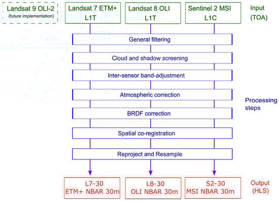
Figure 1.
Workflow to generate Harmonized Landsat-7, Landsat-8, and Sentinel-2 surface reflectance imagery at a 30 m scale. Landsat 9 is planned to be added in the future (dashed box).
- L7-30: ETM+ harmonized surface reflectance resampled to 30 m into the Sentinel-2 tiling system, and adjusted to Sentinel-2 spectral bands.
- L8-30: OLI harmonized surface reflectance resampled to 30 m into the Sentinel-2 tiling system, and adjusted to Sentinel-2 spectral bands.
- S2-30: MSI harmonized surface reflectance resampled to 30 m into the Sentinel-2 tiling system.
Because the L7-30, L8-30, and S2-30 products are gridded to the same resolution and projection system, they are “stackable” (data cube) for time series analysis.
The GEE’s JavaScript code is available as a GEE snapshot (https://code.earthengine.google.com/934b2252c5403a1b3af9a4a0ccb4c9e1, accessed on 22 July 2024) and also at Github (https://github.com/eliasberra/HLS_with_GEE.git, accessed on 22 July 2024).
Specifically, following [5], by “harmonized” it means that the products are as follows:
- Gridded to a common pixel resolution, map projection, and spatial extent.
- Atmospherically corrected to surface reflectance using a common radiative transfer algorithm.
- Normalized to a common nadir view geometry via bidirectional reflectance distribution function (BRDF) estimation.
- Adjusted to represent the response from common spectral bandpasses.
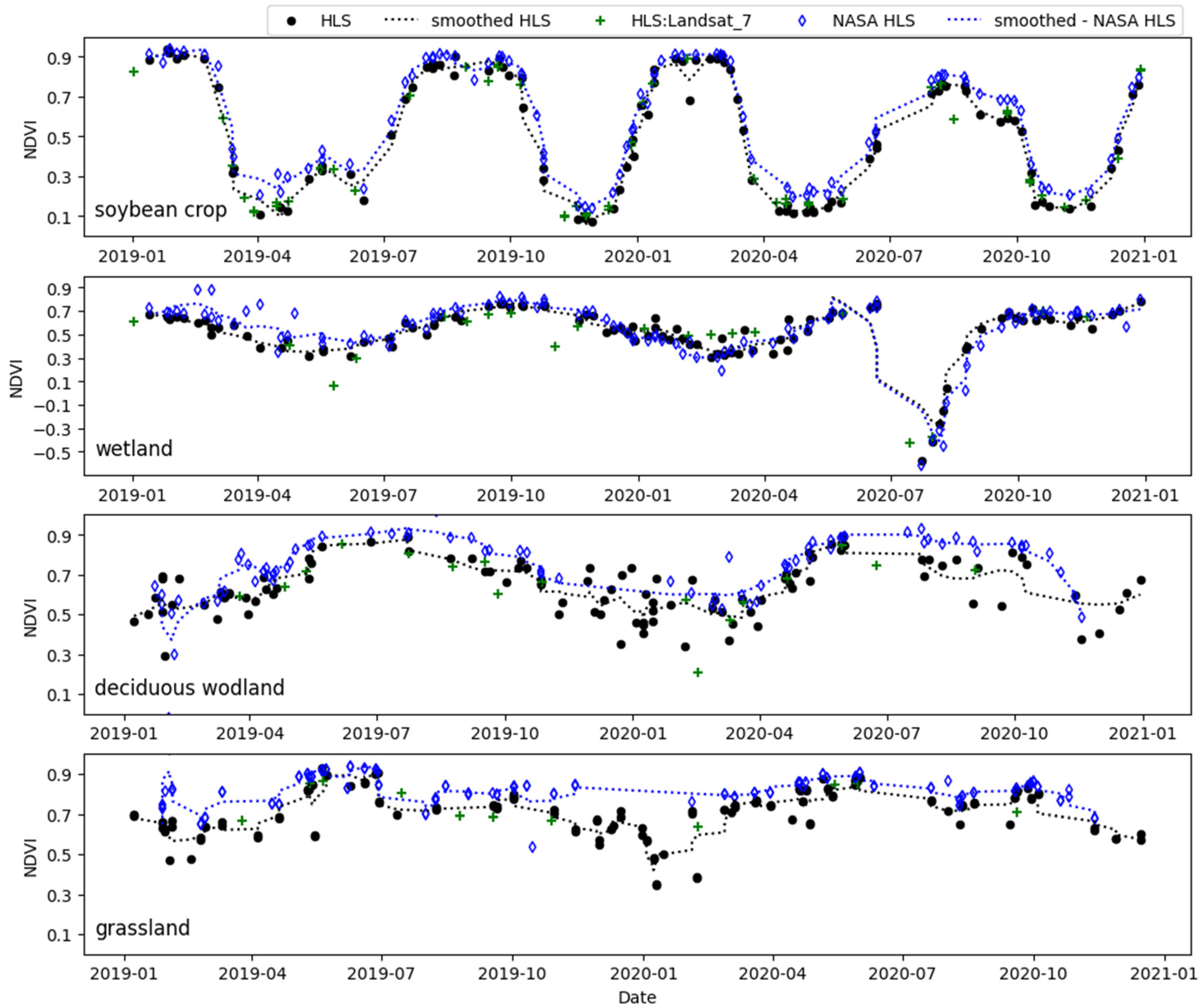
The proposed GEE workflow is applied in two different regions to test the transferability of the methodology and to show other potential applications of HLS series of data (Figure 2). The S2 tiles (S2 scene footprint) are defined as the region of interest to apply our HLS methodology. Firstly, an S2 footprint in southern Brazil was chosen because it intersects ground NDVI data over an agricultural field, data that are used for validation. The second area encompasses an S2 footprint in the northeast UK, from where a well-studied woodland site [4] is selected as an example application. Details of the two sites are given below. Our workflow is applicable worldwide, wherever L7, L8, and S2 data are available (and MODIS, as detailed below).
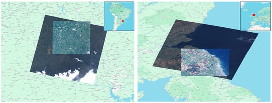
Figure 2.
Study area map showing a test site in southern Brazil and another in northeast UK. Example of a Sentinel-2 scene overlaying a Landsat-8 scene. The base map is the Google Road and the data are projected in WGS 84.
2.1.2. Satellite Data
The input data in the workflow are the top of atmosphere (TOA) reflectance satellite data, which are readily available in the Earth Engine Data Catalogue and are identified as follows:
- L7: “USGS Landsat 7 Collection 2 Tier 1 TOA Reflectance”.
- L8: “USGS Landsat 8 Collection 2 Tier 1 TOA Reflectance”.
- S2: “Harmonized Sentinel-2 MSI: MultiSpectral Instrument, Level-1C”.
Table 1 summarizes the overall characteristics of the three satellites and their sensors and Table 2 summarizes the equivalent bands used in this study. The L7, L8, and S2 satellites are in circular sun-synchronous polar orbits. The L7 satellite is equipped with the ETM+ sensor, which is a fixed whisk-broom multispectral scanning radiometer with seven reflective wavebands (450 nm to 2350 nm) [28]. The L8 has the multispectral OLI push-broom sensor which has nine reflective wavebands (435 nm to 2200 nm) [29]. The same characteristics can be associated with Landsat 9 OLI-2, to be implemented in the future. The S2 mission is composed of two identical satellites, each carrying an MSI push-broom sensor capturing 13 reflective wavebands (443 nm to 2190 nm) [14] at different spatial resolutions; combined, the two out-of-phase S2 satellites provide a nominal revisit time of five days (at the equator) [30]. A more detailed description and intercomparison of these three sensors can be found in [11].

Table 1.
Input sensor specifications [28,29,30,31].
Table 2.
Characteristics of the approximately equivalent Landsat-7 ETM+, Landsat-8 OLI, and Sentinel-2 MSI spectral bands from which the harmonization was applied in this study. The original spatial resolution and central wavelength are given in between brackets [28,29,30,31].
The six approximately equivalent spectral bands between ETM+, OLI, and MSI were used in the HLS workflow: blue, green, red, near infrared (NIR), shortwave-infrared 1 (SWIR1), and shortwave-infrared 2 (SWIR2); the key characteristics are summarized in Table 2. Despite the data gaps in the ETM+ imagery due to the failure of its scan-line corrector (SLC) in 2003 [32], keeping this series of satellite data may be important to increase the series density, especially across areas with frequent cloud cover and prior to launching Sentinel-2.
2.1.3. Inter-Sensor Band Adjustment
The small differences between the equivalent spectral bands can be adjusted if their relationships are known. In this study, setting the S2 MSI as a reference, we adjusted the L7 and L8 TOA reflectance values across the six equivalent bands (blue, green, red, NIR, SWIR1, and SWIR2) using the cross-sensor transformation coefficients derived from [11] (Table 3). Briefly, using over 10,000 image pairs across the conterminous United States, [11] calculated the cross-sensor transformation equations for the six bands, as presented in Table 3.
Table 3.
Cross-sensor transformation coefficients. Sentinel-2 MSI TOA reflectance as a function of Landsat-7 (L7) ETM+ TOA reflectance and Landsat-8 (L8) OLI TOA reflectance, according to [11].
2.1.4. Atmospheric Correction
The Landsat and Sentinel TOA reflectance data were corrected to surface reflectance using the same algorithm to reduce biases that may occur if different algorithms were used [10]. The Sensor Invariant Atmospheric Correction (SIAC) method [33], which has been adapted to the GEE JavaScript language, was used in this study. A detailed description of SIAC is given in [33], including the results of surface reflectance validation for Landsat-8 and Sentinel-2; SIAC has also been successfully tested in [34]. The basic idea of the SIAC method is to use the coarse-resolution spectral BRDF (500 m MODIS BRDF) to provide prior surface reflectance estimation and the Copernicus Atmospheric Monitoring Service (CAMS) 4.4 km data as a prior estimate of atmospheric composition [34]. The surface reflectance is then calculated from the TOA reflectance with the solved atmospheric parameters. Overall, SIAC is a sensor-agnostic approach to atmospheric correction but can only be applied from 2000 onwards, when MODIS data became available. Due to the lack of non-linear solver available in the existing GEE built-in functions, the Aerosol Optical Depth (AOD) estimation is derived from the MCD19A2.061 product, which has been validated to have an accuracy of R = 0.84 and RMSE of 0.12 [35]. Here lies a major difference from the work of [24], who also proposed a method to harmonize L7, L8, and S2 imagery. While we implement a single block of JavaScript code all within the GEE web-based code editor, Nguyen [24]’s workflow performs atmospheric correction (using a different algorithm) outside the GEE environment via Python API and Docker container, a step which may bring extra challenges for the user as it is necessary to install the software and download/upload imagery from/to GEE, therefore diminishing the effectiveness of GEE in terms of being a web-based approach. For this study, all image correction steps were performed using the GEE platform which does not require any external tools to create a streamlined processing pipeline.
Another difference regards the AOD. The algorithm used in [24] assumes that the AOD does not change over the entire region of interest, which may not be valid if a processing is over S2 100 km × 100 km image swath. It uses AOD from MOD08 AOD 550 (‘MODIS/006/MOD08_M3’), which is a monthly mean of the MODIS daily AOD product and does not represent the daily variation of AOD. To enhance these methods, we use the daily MCD19A2.061 product to retrieve AOD, which is a different source, but according to the validation, it produces a high level of accuracy when compared to ground measurements [35] at a higher spatial resolution, 1 km compared to the MOD08’s 1 × 1 degree grid.
2.1.5. Cloud and Cloud Shadow Masking
For L7 and L8, cloud and cloud shadow were identified and masked using the per-pixel bit-packed Quality Assessment Band (BQA) that accompanies the Landsat Collection 1 Level-1 product [36]. BQA is generated with the C Function of Mask (CFMask) algorithm, which is described in [37,38]. Pixels labeled as medium (34–66%) or high (67–100%) confidence cloud, cloud shadow, cirrus, or snow were masked.
For S2, clouds and cloud shadows are identified and masked using the recently available ‘Cloud Score+ S2_HARMONIZED’ product. This dataset includes two QA bands and is produced from the harmonized Sentinel-2 L1C Collection. Cloud Score+ outputs can be used to identify relatively clear pixels and remove clouds and cloud shadows from S2 L1C or S2 L2A imagery. In this study, we used the ‘cs’ QA band, values which are based on a spectral distance between the observed pixel and a (theoretical) clear reference observation [39]. The threshold for masking was set to 0.60, as values between 0.50 and 0.65 generally work well. An overview of the effect of applying the cloud and cloud shadow masking for S2 can be seen in the Appendix A (Figure A1).
2.1.6. View and Illumination Angles (BRDF) Adjustment
The Sentinel-2 and Landsat satellites acquire images at view angles ±10.3° (Sentinel-2) and ±7.5° (Landsat) from nadir that cause small directional effects over non-Lambertian surfaces [40]. Such directional reflectance effects, commonly described by the bidirectional reflectance distribution function (BRDF) (units of sr−1), should be minimized to provide consistent data in applications such as the detection of surface change through space and/or time [40,41]. The BRDF correction of our HLS product was made using the MODIS-based c-factor approach [40,41], because it has been successfully evaluated with L5 TM and L7 ETM+ [41], S2 MSI [40], and S2 and L8 [10] data, and is recommended for view zenith angles near nadir [5]. The technique is deemed conservative, as it under-corrects BRDF effects [42]. The global BRDF coefficients for the isotropic, volumetric, and geometric kernels (definitions in [43]) are shown in Table 4. The technique can only be applied on the L7, L8, and S2 bands equivalent to MODIS ones.
Table 4.
Global 12-month fixed MODIS spectral BRDF model parameters fiso(λ), fgeo(λ), and fvol(λ) used for the c-factor approach [41]. Adapted from [40,41].
The bottom of the atmosphere (BOA) reflectance data are normalized for per-pixel view and per-tile illumination angles, which results in a nadir BRDF-adjusted reflectance (NBAR) product. The view angle (related to the sensor’s FOV) is set to nadir (0° view zenith) and the illumination geometry (zenith and azimuth) is defined based on the tile central latitude (see [5] for the equations). In summary, the NBAR products are surface reflectance normalized for the view and illumination angles. The BRDF correction GEE script was adapted from [24,44].
2.1.7. Spatial Co-Registration between Landsat and Sentinel-2
The objective of our HLS product, and in accordance with [5], is to maintain the geodetic accuracy requirement of the Sentinel-2 images (<20 m error, 2σ) and improve the multi-temporal co-registration between Sentinel-2 and Landsat images (<15 m, 2σ) for the 30 m products. The differences in the geometric reference datasets (among other factors, e.g., different viewing geometries [45]) used to create the S2 and Landsat products lead to residual misregistration between S2 and Landsat data products [46], which may demand a refining of the S2-Landsat registration for multi-sensor time series purposes [47].
The S2 dataset available in the GEE has different geolocation uncertainties as different geometric references are currently used in the series (at the time of writing). Since 30 March 2021 (processing baseline > 03.00), a geometric refinement is applied based on the S2 Global Reference Image (GRI), where preliminary results show an absolute geolocation better than 6 m and a multi-temporal co-registration better than 5 m at 95% confidence [48]. This is notably different from that of the so-called ‘unrefined products’ (no GRI; processing baseline < 03.00), where the absolute geolocation is close to 11 m (at 95%) and the multi-temporal registration is around 12 m (at 95%) for both S2 satellites, in accordance with previous studies [49]. Ongoing efforts are on the way to apply the geometric refinement with GRI to the entire S2 Collection [50].
Both Landsat Collection-1 and Collection-2 products are available in GEE. The Collection-2 data have significant geometric accuracy improvements due to the re-baselining of the Landsat-8 OLI GCPs to the European Space Agency’s Copernicus Sentinel-2 GRI [51]. The independent validation of the Landsat products processed using the GRI dataset indicated a global misregistration error of <8 m (CE90) (Collection-2), an improvement from the 25 m prior to the GRI (Collection-1) [47]. A more recent report calculated a global average registration accuracy of <26 m (CE90) for Landsat Collection-1 data [52]. The Landsat Level-1 (TOA reflectance) is available in both Landsat Collection-1 and Collection-2 within the GEE.
This work tests Landsat Collection-2 data and S2 data with processing baseline prior to 03.00, but the GEE code can be easily adapted to process Collection-1 and/or baseline > 03.00. This means that S2 and Landsat Level-1 products may not align to sub-pixel precision (depending on the Collection/baseline combinations), and may reach misregistration errors of 36–38 m (2σ) in some parts of the globe [5,46]. Therefore, a method to improve the registration between the S2 and Landsat data products is necessary.
In the GEE, the ‘displacement’ function was used to calculate the displacement between a pair of overlapped images (S2/L7 or S2/L8) which were captured at (approximately) the same time over our selected study areas (Table 5). More specifically, the displacement was calculated between pairs of equivalent NIR bands (Table 2). Then, the ‘displace’ function was used to warp and co-register the L7/L8 image to match an S2 (reference) image. Because the S2 absolute geodetic accuracy is better than L7/L8 [48], we aligned all Landsat images using a common base S2. The GEE documentation provides further explanation about the ‘displacement’ and ‘displace’ algorithms; complementarily, Nguyen [24] also provides an interpretation on this.
Table 5.
Pairs of overlapping Sentinel and Landsat imagery, which are cloud-free and acquired on the same date (±2 days) over the study area.
2.1.8. Reproject and Resample
The objective of this step is to put the L7, L8, and S2 data into a common coordinate grid. Our HLS has adopted the tiling system used by the Sentinel-2 Level-1C products, which are composed of granules (also called tiles) of 100 × 100 km ortho-images in the UTM/WGS84 map projection [30]. The S2 tiles (scene footprint; see Figure 2) are defined as the region of interest to apply our HLS methodology.
Because the L7/L8 and S2 data are defined in different tiling schemes with different map projections (UTM zones), the S2 images were reprojected and rescaled (via nearest neighbor) according to the L8/L7 30 m grid (UTM/WGS84), as the HLS result has a 30 m spatial resolution.
2.2. Descriptive and Statistical Analysis
In order to understand the effect of applying our methodology in the satellite data, an analysis was performed in two ways: (i) cross-comparing the TOA reflectance (input data) versus HLS (output) values for each of the equivalent spectral bands, and derived NDVI; (ii) focusing on the red, NIR and NDVI, a detailed cross-comparison of the effect of applying each processing step (Figure 1) in the reflectance and vegetation index values was made. This analysis focuses on comparing L8 × S2, as they are likely of the most relevance for the EO community, but examples are also produced for L7 × S2 (Appendix A). Comparing L8 × L7 was not reliable as their overlapping scenes (one day apart) fall into adjacent paths (border of the images); in addition, the gaps of ETM+ SLC-off images are noticeable along the edge. This resulted in a reduced number of L8 × L7 sampled pixels.
To sample the full range of potential spectral values across the study region (a S2 footprint), a simple random sample of point locations was used. We assembled the images into pairs of observations (S2 × L7, S2 × L8, L7 × L8) that were recorded within 1 day of a different platform-sensor image (e.g., for S2 × L8: an S2 image is paired with an L8 image, only if both images are acquired within ±1 day of each other) to minimize the impact of surface changes between the sensors’ observations. The pixel values that intersected the sample point location, for each of these pairs, were then extracted for the period of 2016–2020; this interval is to restrict the analysis to the S2 processing baseline prior to 03.00 (30 March 2021). These summed up five complete calendar years in which OLI, ETM+, and MSI data were compared. An example of a random sample of point locations can be seen in the Appendix A (Figure A2).
The extracted pixel values were shown on scatterplots. The degree of correspondence between the comparable Sentinel-2 and Landsat (7/8) sensor data was examined by ordinary least square (OLS) regression. The goodness of fit of the OLS regressions was defined by the coefficient of determination (R2). The root mean square difference (RMSD) between Sentinel-2 and Landsat (7 or 8) data was calculated as follows:
where RMSD is the root mean square difference between corresponding Sentinel-2 MSI () and Landsat () reflectance or NDVI values at every ith observation, out of n observations.
2.3. Ground Reference Data
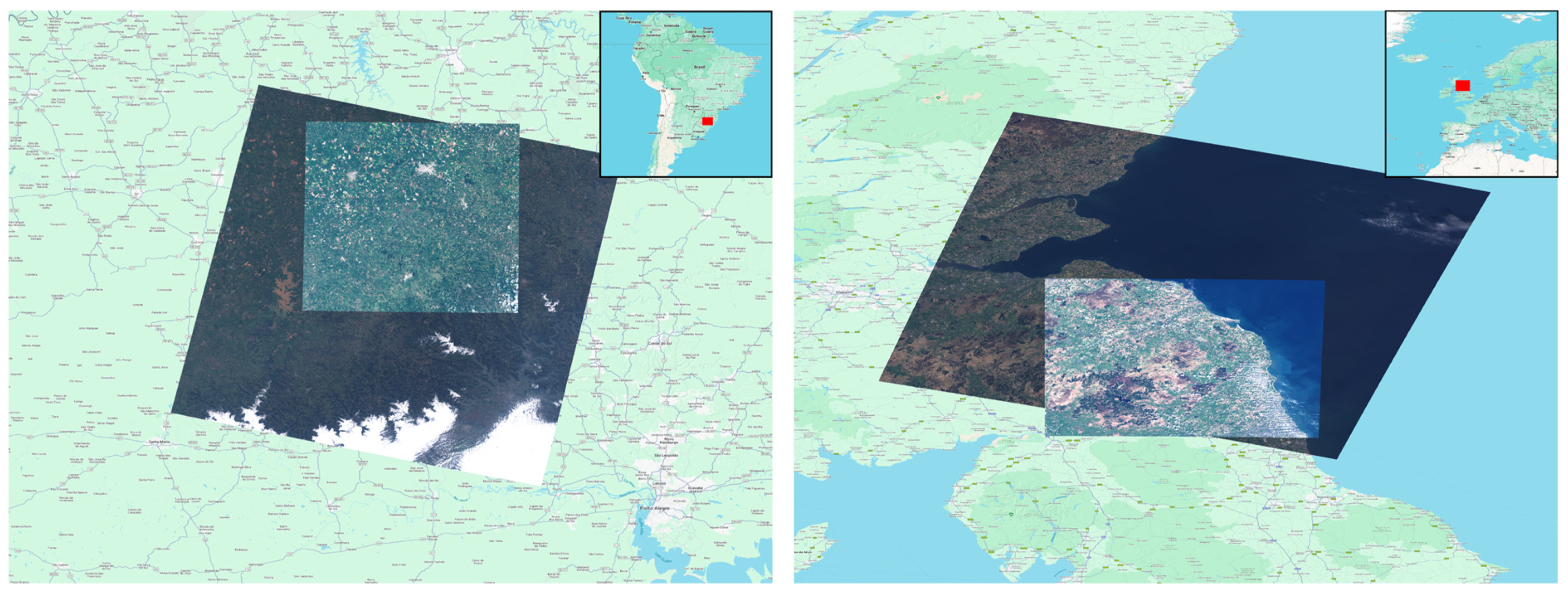
The performance of our HLS surface reflectance product was evaluated by cross-comparing its HLS series values against independent in situ NDVI data at an agricultural field in southern Brazil (−28.228550°, −52.905090°). Ground NDVI measurements were retrieved from a couple of Spectral Reflectance Sensors (SRS—Decagon Devices, Inc., Pullman, WA, USA) (Figure 3), as described and validated in [53,54]. Briefly, the NDVI sensors are of two types. While the incident radiation was measured with an NDVI-hemispherical (up looking), the surface-reflected radiance was measured by an NDVI field stop (down looking). Both NDVI sensors measure the red and near-infrared spectra. The sensors provide continuous monitoring with recordings every 15 minutes, data which were stored with a CR1000 datalogger (Campbell Scientific, Inc., Logan, UT, USA). These NDVI sensors were installed in pairs at a height of 1 m above the soybean canopy.

Figure 3.
Ground NDVI sensors installed in a soybean plantation, crop season 2017/2018.
2.4. Application Examples and Comparison with NASA HLS
The processing power of the developed framework is exemplified with four potential applications (four different land cover types) across the two test sites (Figure 2). Two examples are from southern Brazil: (i) an agricultural field to illustrate a crop monitoring application (same site where the ground NDVI data were available); and (ii) a wetland to illustrate a dynamic monitoring of wetlands and inundations (−28.49785°, −52.55475°). The other examples come from the northeast UK: (iii) a woodland site with deciduous-dominated tree species to illustrate a forest phenology monitoring (55.22055°, −1.69610°); and, (iv) a grassland to illustrate the temporal patterns of grassland dynamics (54.98799°, −2.60930°).
At these four sites, the HLS time series examples were extracted and graphs were produced. Our GEE-generated HLS was also intercompared with the existing NASA HLS data [20,21] to evaluate their degree of agreement in terms of magnitude of values and temporal trajectories. The NASA HLS product was downloaded using the Application for Extracting and Exploring Analysis Ready Samples (AppEEARS) [55], which is a web-based application that allows extracting the NASA HLS point samples of geographic coordinates. Only harmonized observations flagged without clouds (‘Fmask_Cloud_Description’ = No) were used in the comparisons with our HLS. It is important to remember that the NASA HLS does not harmonize Landsat 7 data.
3. Results
The cross-comparison of Landsat-8 vs. Sentinel-2 equivalent spectral bands and derived NDVI values, before (input) and after (output) applying the HLS method, is shown in Figure 4, while Figure 5 shows how the HLS workflow affects the red, NIR, and NDVI values for each processing step. A similar comparison for Landsat-7 vs. Sentinel-2 can be seen in the Appendix A (Figure A3 and Figure A4).
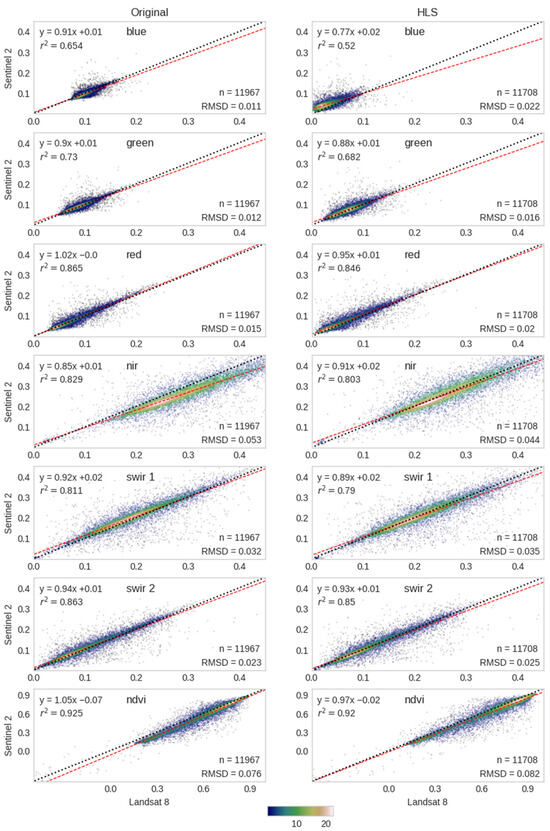
Figure 4.
Cross-comparison of Landsat-8 vs. Sentinel-2 reflectance and derived NDVI values, before (‘Original’ column) and after applying the HLS method. The pairs are made of observations recorded within 1 day of difference (1 January 2016 and 31 December 2020). The red dashed lines are fitted using ordinary least squares (OLS) regression with equations shown in the top left. The dotted black lines are 1:1 lines superimposed for reference. The plot colors show the relative density of occurrence of similar pixel values with the legend shown in the bottom.
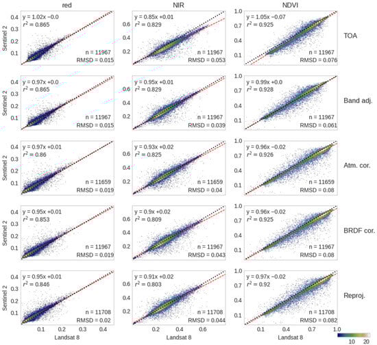
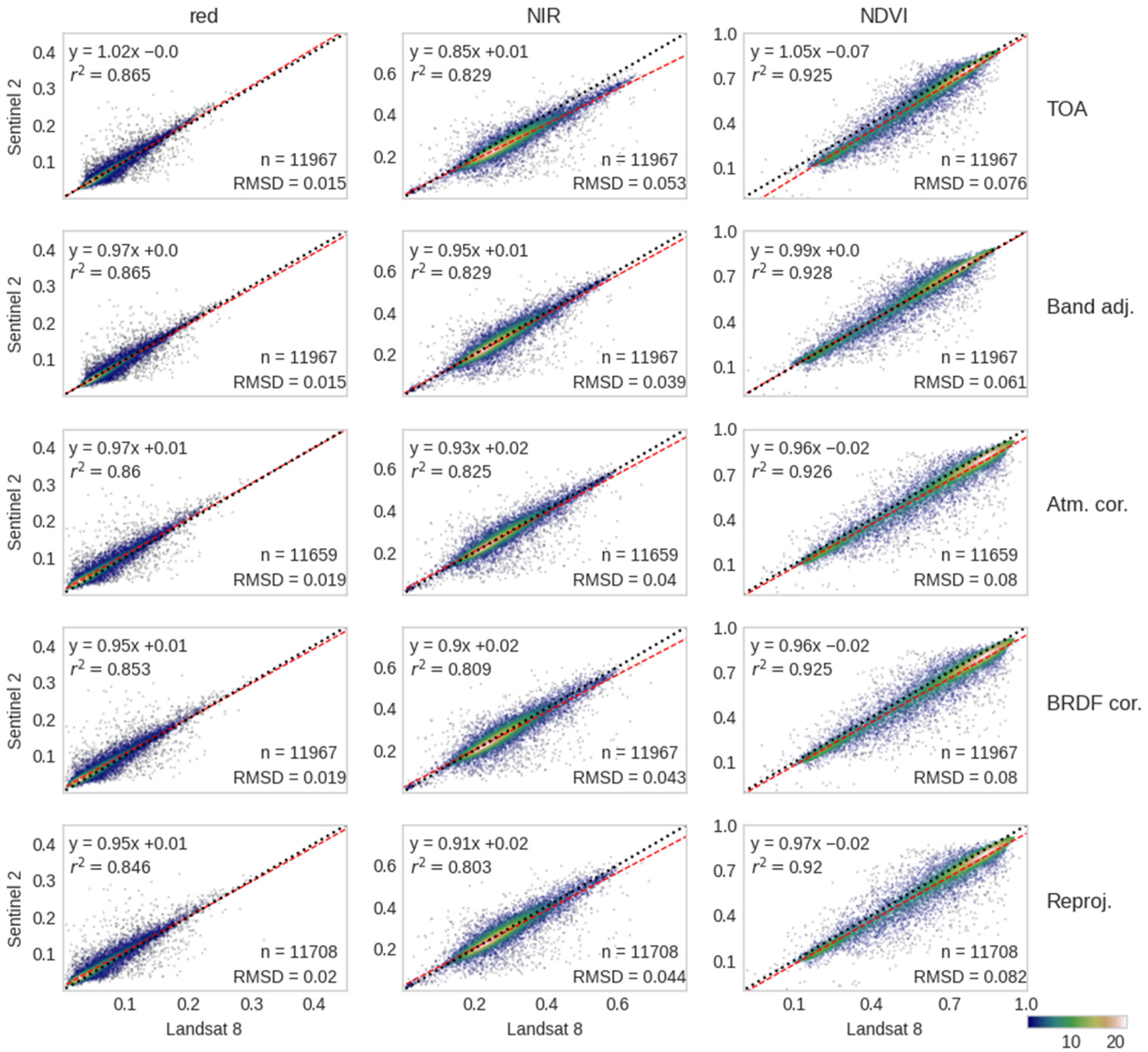
Figure 5.
Cross-comparison of Landsat-8 vs. Sentinel-2 reflectance (red and NIR bands) and derived NDVI values for each processing step used in this study. The pairs are made of observations recorded within 1 day of difference (1 January 2016 and 31 December 2020). The red dashed lines are fitted using ordinary least squares (OLS) regression with equations shown in the top left. The dotted black lines are 1:1 lines superimposed for reference. The plot colors show the relative density of occurrence of similar pixel values with the legend shown in the bottom right.
A shift towards smaller reflectance values and increasing in the data range occur particularly and most noticeably in the shortest wavelengths (blue, green, and red; Figure 4). This has been seen in similar studies [10,56] and is expected as the atmospherically corrected results compensate for the additive components and aerosol absorption of the atmosphere (see ‘Atm. cor.’ in Figure 5). The lowest correlations are also seen in the shortest wavelength band (blue in Figure 4; R2 = 0.65 and R2 = 0.52), which is also likely due to its higher sensitivity to such atmospheric influence.
Except for the blue band, the agreement metrics (R2, RMSD, and regression slope) values are about the same when comparing ‘Original’ (TOA reflectance) vs. ‘HLS’ (harmonized NBAR at 30 m) for L8 × S2 (Figure 4). The best agreements are observed with NDVI with both ‘Original’ and ‘HLS’ products, with the NDVI HLS regression slope being closer to the 1:1 line. This is expected as the normalized difference between red and NIR-retrieved surface reflectance (NDVI) tends to be less affected by changes in illumination conditions [57], BRDF effects, and other geometric and inter-sensor specific differences, than the individual bands alone [10,58].
Except for the blue and green band, all of the OLS regressions had good fits for the original (0.81 ≤ R2 ≥ 0.92) and HLS (0.79 ≤ R2 ≤ 0.92) products (Figure 4). Similarly, all of the OLS regressions had good fits for red and NIR reflectance (R2 ≥ 0.80) and NDVI (R2 ≥ 0.92) comparisons, across the different processing steps of our workflow (Figure 5).
3.1. Comparing with Ground NDVI
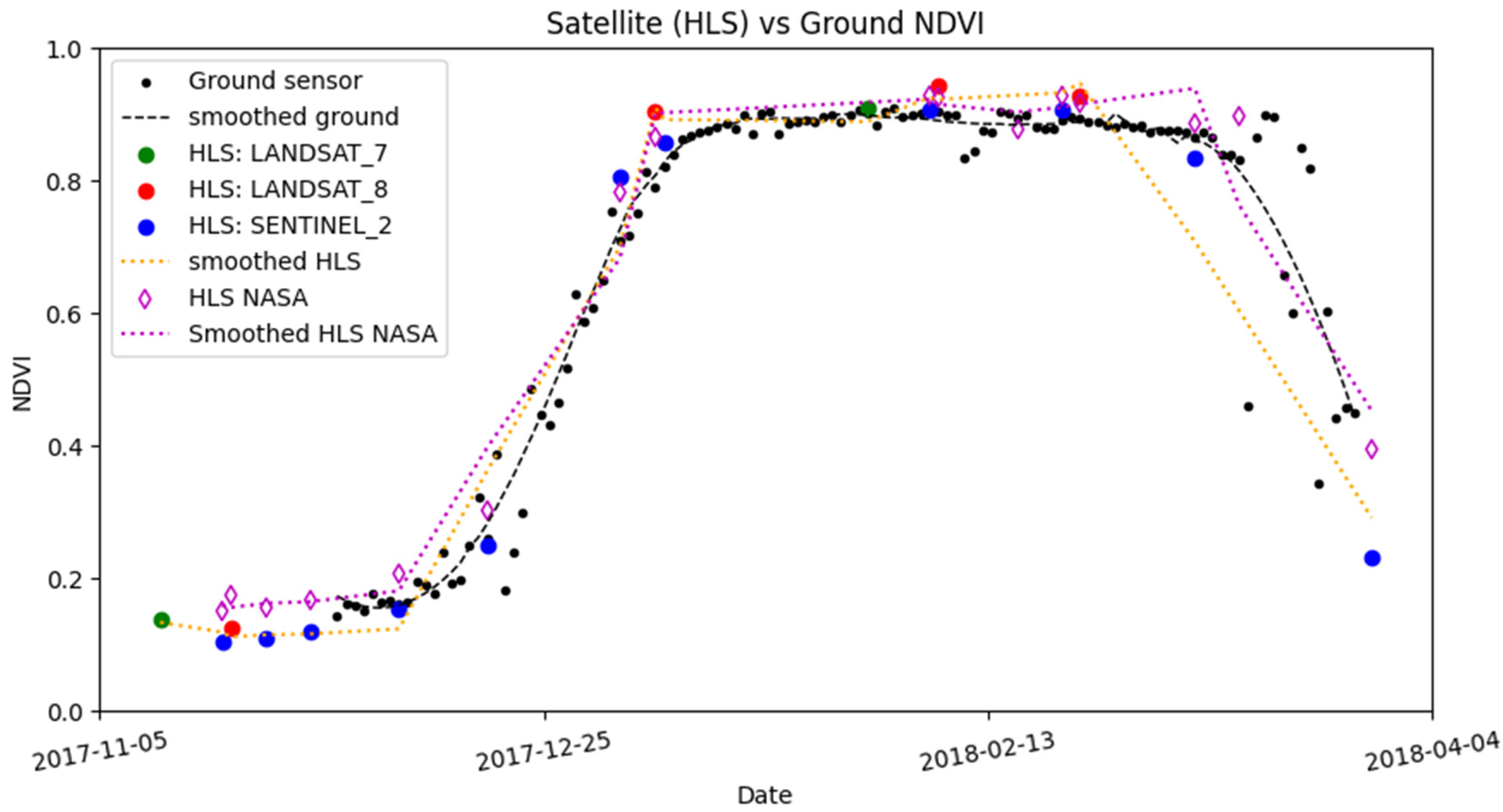
The magnitudes of the ground (considered as reference) and our harmonized satellite NDVI values are all very close (R2 = 0.98; N = 11; when considering only pairs of coinciding HLS and ground NDVI), following very similar temporal trajectories for the soybean plantation (not smoothed data; Figure 6). Some differences arise when comparing the two smoothed series as the satellite series contains relatively larger temporal gaps, when compared to the daily ground NDVI. Most of the data points come from Sentinel-2 (11/17), followed by Landsat-8 (4/17) and Landsat-7 (2/17).
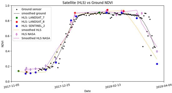
Figure 6.
Harmonized Landsat Sentinel (HLS) vs. ground NDVI at an agricultural field in southern Brazil. The HLS data points are colored accordingly to their original satellite types. The NASA HLS is also overlaid for comparison purposes. A second-order Savitzky-Golay filter was applied to the ground (window size = 30) and satellite (window size = 5) time series data.
Regarding the NASA HLS data, very similar values and temporal dynamics are observed when comparing against our HLS. Equally, NASA HLS values are in good agreement with the ground NDVI (R2 = 0.99; N = 11).
3.2. Example of Applications
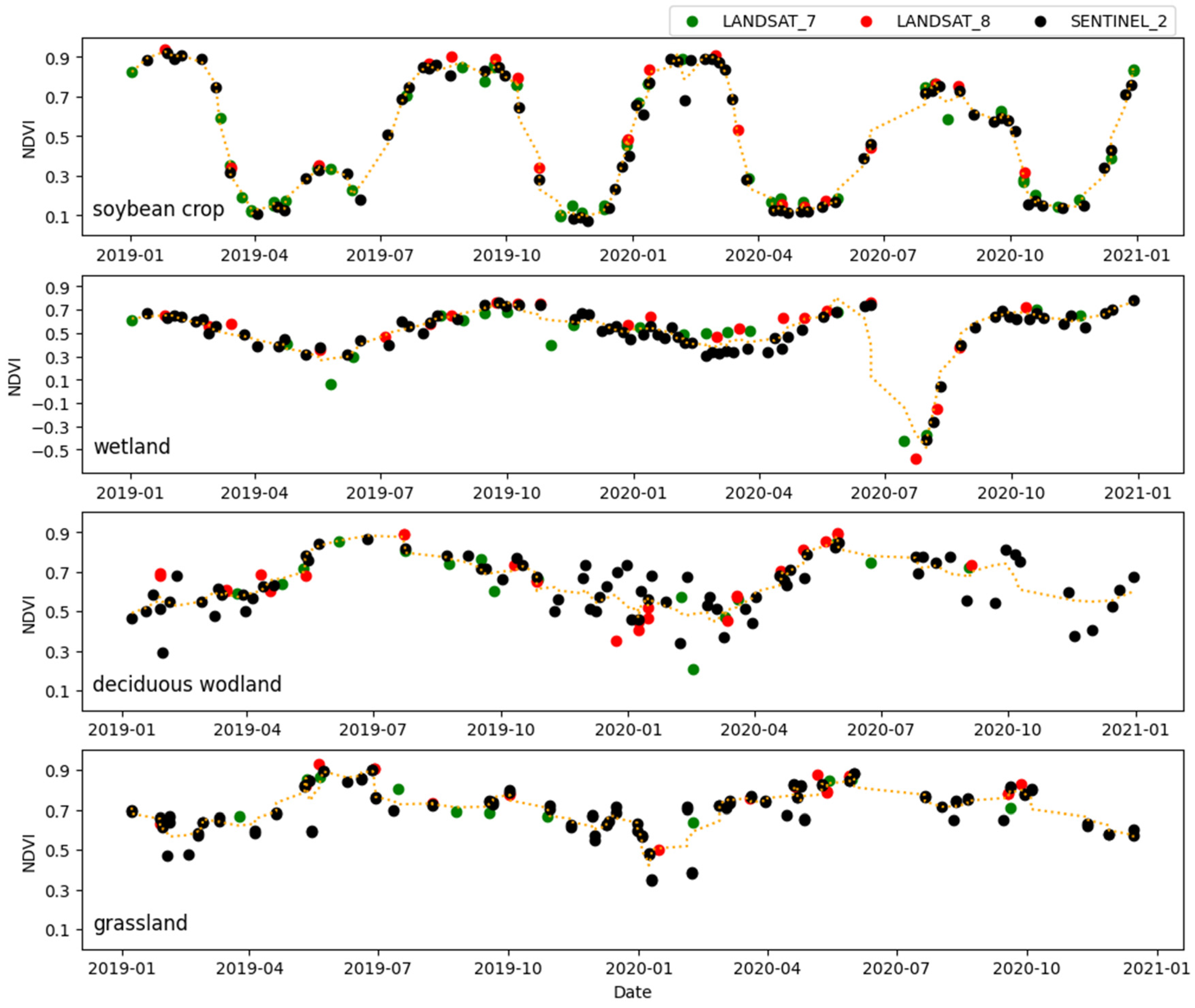
A longer time series example of HLS-derived NDVI time series is shown in Figure 7. The subtropical agricultural fields (Brazil) have shorter seasons, while the woodland with mixed deciduous trees (UK) and the grassland (UK) have longer seasons. The time series from the wetland (Brazil) has a pronounced drop in NDVI values due to episodic inundation events covering its vegetation. There is a noticeable increase in the number of good quality observations after Sentinel-2 became fully operational, particularly during the period of 2016–2017 (Figure A5). Figure 6 and Figure 7 show that the Landsat 7 data, despite their technical challenges, can be very useful to increase the temporal frequency of the series, particularly before the Sentinel-2 constellation (A and B) became fully operational in mid-2017 (Figure A5).
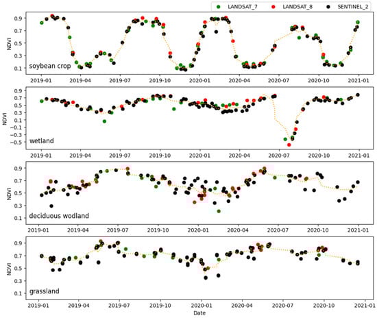
Figure 7.
Harmonized Landsat Sentinel (HLS) example time series at (from top to bottom) an agricultural field where soybean is usually grown, a wetland (in southern Brazil), a deciduous tree-dominated woodland, and a grassland (in northeast UK). The HLS data points are colored accordingly to their original satellite types. A second-order Savitzky–Golay filter (dotted line) was applied to the crop (window size = 5), wetland, woodland, and grassland (window size = 10) time series data.
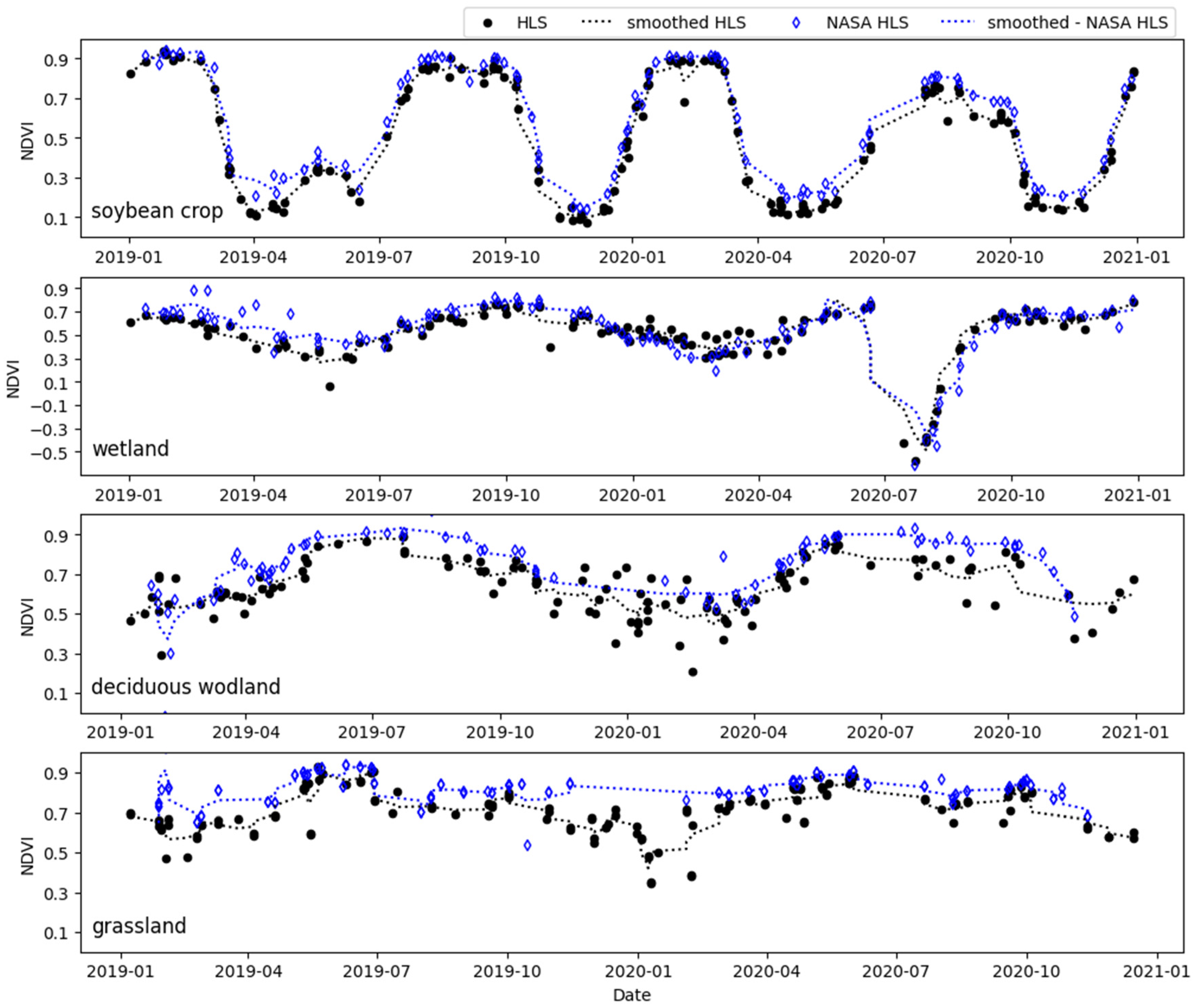
Overall, our GEE HLS and the NASA HLS time series follow a very similar temporal trajectory of NDVI data (Figure 8). The intercomparison showed a closer agreement in the sampled series from southern Brazil (crop: R2 = 0.99; N = 102; wetland: R2 = 0.85; N = 108) than the series from the UK (woodland: R2 = 0.61; N = 80; grassland: R2 = 0.75; N = 204). In terms of absolute NDVI values, the degree of correspondence varies depending on the site and time of year. A more pronounced difference is observed in the UK sites around January 2020 (wintertime). While our HLS retrieved a denser (yet noisier) time series, the NASA HLS product resulted in fewer data points. Additionally, the Landsat 7 data remain valuable during periods when high-quality L8 and S2 observations are unavailable (see Figure A6), thereby enhancing the density of the time series.
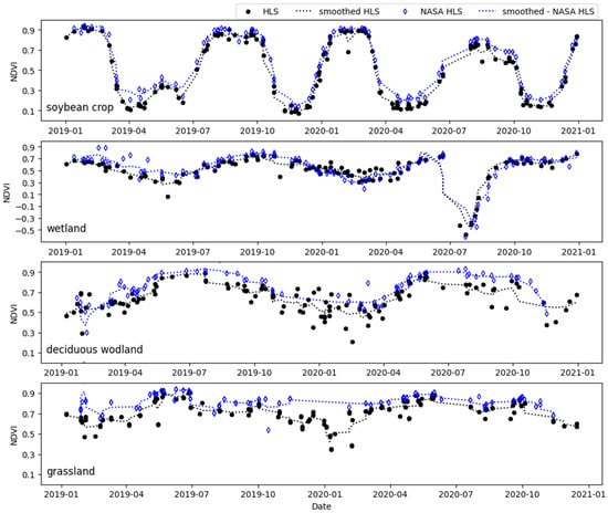
Figure 8.
Comparison between our HLS and the NASA HLS across four different land cover types in southern Brazil (crop and wetland) and northeast UK (woodland and grassland). A second-order Savitzky–Golay filter (dotted line) was applied to the crop (window size = 5), wetland, woodland, and grassland (window size = 10) time series data.
4. Discussion
In this study, we used GEE, a cloud computing platform, to develop an all-in-one web-based workflow to produce 30 m harmonized surface reflectance data from L7 ETM+, L8 OLI, and S2 MSI top of atmosphere reflectance data. The greatest benefit of our HLS product is a denser temporal resolution of optical data compared to a single satellite sensor alone. The additional temporal resolution provided by HLS products, like our workflow and other initiatives [5], can enhance observation-intensive methods in applications such as land surface phenology [1,58,59], agricultural phenology, crop monitoring, burned area mapping [42], land use and land cover mapping, and near real-time land cover change [60]. For vegetation phenology studies using medium spatial resolution satellites, this is particularly important as image availability can be significantly reduced due to cloud contamination, reducing the already lower dataset temporal resolution (compared to coarse spatial resolution), resulting in large temporal gaps and increasing prediction uncertainties of phenological metrics and trends [4,61].
The cross-comparison of HLS datasets from Landsat-8 and Sentinel-2 revealed overall good agreements between the equivalent spectral bands (except the blue band), but differences remained. In [10], the authors quantified uncertainties due only to spectral response function differences between Sentinel-2A MSI and Landsat-8 OLI, but only small disagreements were observed for reflectance across the equivalent spectral bands (RMSD < 0.015) and NDVI (RMSD = 0.0151). In [62], the authors found significant differences between MSI and ETM+ simulated images (from Airborne Prism Experiment (APEX)) across red, near infrared, and NDVI spectral values; the RMSE values ranged from greater than 8% in the red band to 2.3% in the NIR band, and an RMSE = 3.1% between NDVI values.
Our workflow would benefit from cross-sensor transformation coefficients developed specifically for our NBAR products (after BRDF correction) to diminish small non-random differences (e.g., residual calibration errors [63]) of coincident Landsat ETM+, Landsat OLI, and Sentinel MSI NBAR data. The development of such new correction factors’ coefficients for all comparable bands was beyond the scope of this study, as a systematic and geographically extensive investigation would be necessary to produce robust coefficients, as in [11] for TOA coefficients. Nevertheless, site-specific models could be developed for specific areas of study in a future version of our workflow, as in [12] and [10].
The spatial co-registration step in the GEE may be optional as both Landsat and Sentinel-2 datasets are expected to be processed using a common geometric reference in the near future: the GRI. Updated Collection 2 results (Phase 4) have yielded a Landsat/Sentinel-2 global average registration accuracy of <10 meters circular error at the 90th percentile (CE90) [52]. This substantial improvement in the Landsat/Sentinel-2 registration accuracy is expected to satisfy the geometric requirements of the analysis ready data [47].
The degree of correspondence between our HLS and NASA HLS datasets varied depending on the site and time of year. In the Brazilian subtropical land cover types (~28° S latitude), the agreements between the two HLS were good, whereas greater differences were observed in the UK land covers (~55° N latitude), mainly within the UK wintertime. The differences in atmospheric and illumination conditions are likely contributing to such differences, as the UK experiences frequent cloud cover (and its shadow) and haze [64] and a higher solar zenith angle (stronger directional and angular effects [65]). Also, the atmospheric threshold that we used in the NASA HLS seems more conservative, leading to a lower number of selected samples (Brazil: N = 191; UK: N = 202) when compared to our product (Brazil: N = 266; UK: N = 266). The combined effect of using different cloud/cloud shadows and atmospheric and BRDF correction methods between our HLS and NASA HLS workflows has also likely contributed to observed differences.
Currently, our workflow is designed to harmonize ETM+, OLI, and MSI image data only at local scales (S2 footprint) to overcome the processing limitations imposed by the GEE platform (for a comprehensive overview of GEE limitations, please see [66]). In this first version, our focus was to assemble an operational, yet scientifically sound, HLS workflow. Applying the workflow to larger extents (regional scales) is a known challenge that may be tackled in a subsequent version of the workflow. Planned improvements to the workflow are the following: (i) adding the Landsat 9 dataset in order to increase the HLS virtual constellation and keeping the HLS updated; (ii) adding a topographic correction algorithm, such as the [67] method or the c-factor method by [68]; (iii) a more comprehensive intercomparison of our NBAR product against the ground/reference reflectance from the RadCalNet sites [33] and with the existing NASA HLS data.
5. Conclusions
This paper presents a workflow for the harmonization of Landsat and Sentinel-2 (HLS) data into the GEE cloud platform. The GEE JavaScript code used to implement the HLS methodology is available and may allow the reproducibility of a harmonized product within a user-defined area of interest.
The HLS dataset results in a denser image time series at a 30-meter scale, imagery which may be useful for applications demanding the detection of rapid changes on the land surface.
With the increasing number of Earth observation satellites providing free imagery archives at medium spatial resolution, combining multiple satellite observations into a single dataset can significantly enhance temporal resolutions, improving our ability to detect fine-grained, subtle landscape change patterns.
Author Contributions
Conceptualization, E.F.B. and D.C.F.; methodology, E.F.B. and F.Y.; software, E.F.B. and F.Y.; validation, E.F.B.; formal analysis, E.F.B.; resources, E.F.B. and F.Y.; data curation, E.F.B. and F.Y.; writing—original draft preparation, E.F.B.; writing—review and editing, E.F.B., F.M.B., D.C.F., and F.Y.; visualization, E.F.B. and F.M.B.; supervision, E.F.B.; funding acquisition, E.F.B. and F.Y. All authors have read and agreed to the published version of the manuscript.
Funding
The work of E. F. Berra was supported by the Conselho Nacional de Desenvolvimento Científico e Tecnológico (CNPq), grant 150486/2019-7 and by the Fundação Araucária, grant PI 13/2022 (protocol number UFP2022251000030). Fabio M. Breunig would like to thank CNPq, grant 305452/2023-1. Feng Yin is grateful to the Natural Environment Research Council’s (NERC) National Centre for Earth Observation (NCEO) for financial support under grant PR140015, with additional support from the Science and Technology Facilities Council (STFC) UK-Newton Agritech Programme, project number 533651, AgZero+ research programme (NE/W005050/1), and NERC CPEO programme, project reference NE/X006328/1.
Data Availability Statement
Data are contained within the article.
Acknowledgments
The authors would like to thank Google for keeping up and running the Google Earth Engine. The authors are also grateful to the reviewers for their useful suggestions.
Conflicts of Interest
The authors declare no conflicts of interest.
Appendix A
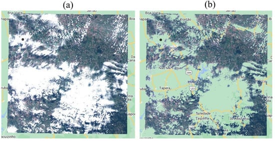
Figure A1.
Example of the cloud and cloud shadow masking algorithm used in this study. The image shows a Sentinel-2 image (GEE id: “COPERNICUS/S2_HARMONIZED/20190503T133229_20190503T133232_T22JCP”) before (a) and after (b) applying the mask.
Figure A1.
Example of the cloud and cloud shadow masking algorithm used in this study. The image shows a Sentinel-2 image (GEE id: “COPERNICUS/S2_HARMONIZED/20190503T133229_20190503T133232_T22JCP”) before (a) and after (b) applying the mask.

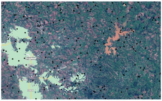
Figure A2.
Example of a random sample of point locations used in this study. This was performed using the GEE function ‘ee.FeatureCollection.randomPoints()’. The background is a Sentinel-2 (id: ‘COPERNICUS/S2_HARMONIZED/20170617T133221_20170617T133702_T22JCP’) true-color composite after cloud and cloud shadow masking.
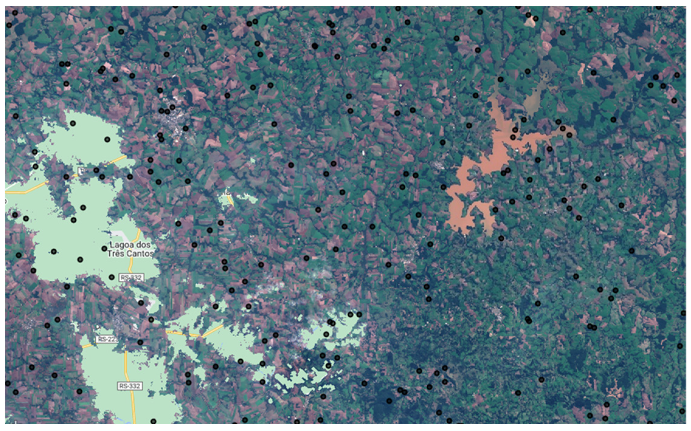
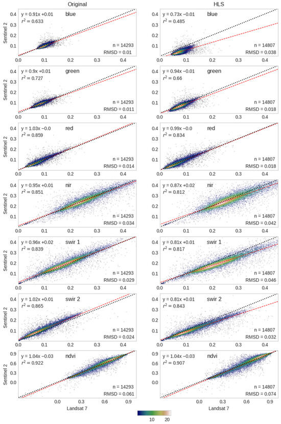
Figure A3.
Cross-comparison of Landsat-7 vs. Sentinel-2 reflectance and derived NDVI values, before (‘Original’ column) and after applying the HLS method. The pairs are made of observations recorded within 1 day of difference (1 January 2016 and 31 December 2020). The red dashed lines are fitted using ordinary least squares (OLS) regression with equations shown in the top left. The dotted black lines are 1:1 lines superimposed for reference. The plot colors show the relative density of occurrence of similar pixel values with the legend shown in the bottom right.
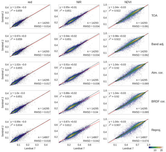
Figure A4.
Cross-comparison of Landsat-7 vs. Sentinel-2 reflectance (red and NIR bands) and derived NDVI values for each processing step used in this study. The pairs are made of observations recorded within 1 day of difference (1 January 2016 and 31 December 2020). The red dashed lines are fitted using ordinary least squares (OLS) regression with equations shown in the top left. The dotted black lines are 1:1 lines superimposed for reference. The plot colors show the relative density of occurrence of similar pixel values with the legend shown in the bottom right.
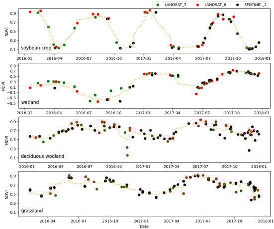
Figure A5.
Harmonized Landsat Sentinel (HLS) example time series (2016–2017) at (from top to bottom) an agricultural field where soybean is usually grown, a wetland (in southern Brazil), a deciduous tree-dominated woodland, and a grassland (in northeast UK). The HLS data points are colored accordingly to their original satellite types. A second-order Savitzky–Golay filter (dotted line) was applied to the crop (window size = 5), woodland, grassland, and wetland (window size = 30) time series data.
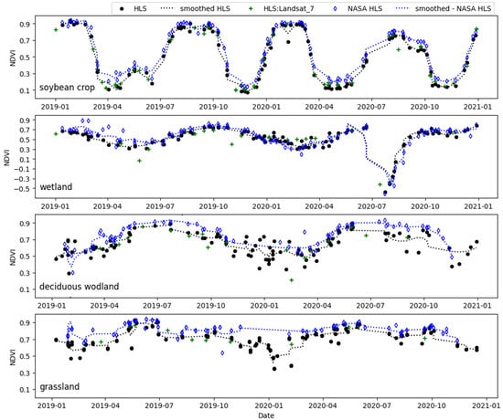
Figure A6.
Comparison between our HLS and the NASA HLS across different land cover types in southern Brazil (crop and wetland) and northeast UK (woodland and grassland). In this comparison, the Landsat 7 data from our HLS are not considered when smoothing the time series of data. A second-order Savitzky–Golay filter (dotted line) was applied to the crop (window size = 5), wetland, woodland, and grassland (window size = 10) time series data.
References
- Bolton, D.K.; Gray, J.M.; Melaas, E.K.; Moon, M.; Eklundh, L.; Friedl, M.A. Continental-scale land surface phenology from harmonized Landsat 8 and Sentinel-2 imagery. Remote Sens. Environ. 2020, 240, 111685. [Google Scholar] [CrossRef]
- Sun, L.; Gao, F.; Xie, D.; Anderson, M.; Chen, R.; Yang, Y.; Chen, Z. Reconstructing daily 30 m NDVI over complex agricultural landscapes using a crop reference curve approach. Remote Sens. Environ. 2020, 253, 112156. [Google Scholar] [CrossRef]
- Chaves, M.E.D.; Picoli, M.C.A.; Sanches, I.D. Recent Applications of Landsat 8/OLI and Sentinel-2/MSI for Land Use and Land Cover Mapping: A Systematic Review. Remote Sens. 2020, 12, 3062. [Google Scholar] [CrossRef]
- Berra, E.F.; Gaulton, R.; Barr, S. Assessing spring phenology of a temperate woodland: A multiscale comparison of ground, unmanned aerial vehicle and Landsat satellite observations. Remote Sens. Environ. 2019, 223, 229–242. [Google Scholar] [CrossRef]
- Claverie, M.; Ju, J.; Masek, J.G.; Dungan, J.L.; Vermote, E.F.; Roger, J.-C.; Skakun, S.V.; Justice, C. The Harmonized Landsat and Sentinel-2 surface reflectance data set. Remote Sens. Environ. 2018, 219, 145–161. [Google Scholar] [CrossRef]
- Moreno-Martínez, Á.; Izquierdo-Verdiguier, E.; Maneta, M.P.; Camps-Valls, G.; Robinson, N.; Muñoz-Marí, J.; Sedano, F.; Clinton, N.; Running, S.W. Multispectral high resolution sensor fusion for smoothing and gap-filling in the cloud. Remote Sens. Environ. 2020, 247, 111901. [Google Scholar] [CrossRef] [PubMed]
- Frantz, D. FORCE—Landsat + Sentinel-2 Analysis Ready Data and Beyond. Remote Sens. 2019, 11, 1124. [Google Scholar] [CrossRef]
- NASA. Harmonized Landsat and Sentinel-2. Available online: https://hls.gsfc.nasa.gov/ (accessed on 7 February 2021).
- Li, J.; Roy, D.P. A Global Analysis of Sentinel-2A, Sentinel-2B and Landsat-8 Data Revisit Intervals and Implications for Terrestrial Monitoring. Remote Sens. 2017, 9, 902. [Google Scholar] [CrossRef]
- Zhang, H.K.; Roy, D.P.; Yan, L.; Li, Z.; Huang, H.; Vermote, E.; Skakun, S.; Roger, J.-C. Characterization of Sentinel-2A and Landsat-8 top of atmosphere, surface, and nadir BRDF adjusted reflectance and NDVI differences. Remote Sens. Environ. 2018, 215, 482–494. [Google Scholar] [CrossRef]
- Chastain, R.; Housman, I.; Goldstein, J.; Finco, M.; Tenneson, K. Empirical cross sensor comparison of Sentinel-2A and 2B MSI, Landsat-8 OLI, and Landsat-7 ETM+ top of atmosphere spectral characteristics over the conterminous United States. Remote Sens. Environ. 2018, 221, 274–285. [Google Scholar] [CrossRef]
- Flood, N. Comparing Sentinel-2A and Landsat 7 and 8 Using Surface Reflectance over Australia. Remote Sens. 2017, 9, 659. [Google Scholar] [CrossRef]
- Mandanici, E.; Bitelli, G. Preliminary Comparison of Sentinel-2 and Landsat 8 Imagery for a Combined Use. Remote Sens. 2016, 8, 1014. [Google Scholar] [CrossRef]
- Drusch, M.; Del Bello, U.; Carlier, S.; Colin, O.; Fernandez, V.; Gascon, F.; Hoersch, B.; Isola, C.; Laberinti, P.; Martimort, P.; et al. Sentinel-2: ESA’s Optical High-Resolution Mission for GMES Operational Services. Remote Sens. Environ. 2012, 120, 25–36. [Google Scholar] [CrossRef]
- Wulder, M.A.; Hilker, T.; White, J.C.; Coops, N.C.; Masek, J.G.; Pflugmacher, D.; Crevier, Y. Virtual constellations for global terrestrial monitoring. Remote Sens. Environ. 2015, 170, 62–76. [Google Scholar] [CrossRef]
- Kington, J.; Collison, A. Scene Level Normalization and Harmonization of Planet Dove Imagery. February 2022. Available online: https://assets.planet.com/docs/scene_level_normalization_of_planet_dove_imagery.pdf (accessed on 19 May 2024).
- Peng, D.; Wang, Y.; Xian, G.; Huete, A.R.; Huang, W.; Shen, M.; Wang, F.; Yu, L.; Liu, L.; Xie, Q.; et al. Investigation of land surface phenology detections in shrublands using multiple scale satellite data. Remote Sens. Environ. 2020, 252, 112133. [Google Scholar] [CrossRef]
- Ju, J.; Masek, J.G. Harmonized Landsat Sentinel-2 (HLS) Product User Guide Product Version 2.0. 2024. Available online: https://lpdaac.usgs.gov/products/hlsl30v002/ (accessed on 17 June 2024).
- Masek, J.G.; Ju, J. HLS Sentinel-2 MSI Surface Reflectance Daily Global 30 m V1.5. NASA EOSDIS Land Processes DAAC. Available online: https://lpdaac.usgs.gov/products/hlss30v015/ (accessed on 23 February 2021).
- Masek, J.G.; Ju, J. HLS Sentinel-2 MSI Surface Reflectance Daily Global 30m v2.0. Available online: https://lpdaac.usgs.gov/products/hlss30v002/ (accessed on 17 June 2024).
- Masek, J.G.; Ju, J. HLS Operational Land Imager Surface Reflectance and TOA Brightness Daily Global 30 m v2.0. Available online: https://cmr.earthdata.nasa.gov/search/concepts/C2021957657-LPCLOUD/35 (accessed on 17 June 2024).
- Saunier, S.; Louis, J.; Debaecker, V.; Beaton, T.; Cadau, E.G.; Boccia, V.; Gascon, F. Sen2like, A Tool To Generate Sentinel-2 Harmonised Surface Reflectance Products—First Results with Landsat-8. In Proceedings of the IGARSS 2019—2019 IEEE International Geoscience and Remote Sensing Symposium, Yokohama, Japan, 28 July–2 August 2019; IEEE: Piscataway, NJ, USA, 2019; pp. 5650–5653. [Google Scholar]
- Saunier, S.; Louis, J.; Gascon, F.; Cadau, E.G.; Debaecker, V.; Claverie, M.; Boccia, V. Sentinel-2 Harmonised Surface Reflectance Products with Sen2like. Phase 1 status. In Proceedings of the ESA PHI WEEK 2020, Virtual, 28 September–2 October 2020; p. 21. [Google Scholar] [CrossRef]
- Nguyen, M.D.; Baez-Villanueva, O.M.; Bui, D.D.; Nguyen, P.T.; Ribbe, L. Harmonization of Landsat and Sentinel 2 for Crop Monitoring in Drought Prone Areas: Case Studies of Ninh Thuan (Vietnam) and Bekaa (Lebanon). Remote Sens. 2020, 12, 281. [Google Scholar] [CrossRef]
- Sudmanns, M.; Tiede, D.; Lang, S.; Bergstedt, H.; Trost, G.; Augustin, H.; Baraldi, A.; Blaschke, T. Big Earth data: Disruptive changes in Earth observation data management and analysis? Int. J. Digit. Earth 2020, 13, 832–850. [Google Scholar] [CrossRef] [PubMed]
- Descalsferrando, A.; Verger, A.; Yin, G.; Penuelas, J. A Threshold Method for Robust and Fast Estimation of Land-Surface Phenology Using Google Earth Engine. IEEE J. Sel. Top. Appl. Earth Obs. Remote Sens. 2020, 14, 601–606. [Google Scholar] [CrossRef]
- Gorelick, N.; Hancher, M.; Dixon, M.; Ilyushchenko, S.; Thau, D.; Moore, R. Google Earth Engine: Planetary-scale geospatial analysis for everyone. Remote Sens. Environ. 2017, 202, 18–27. [Google Scholar] [CrossRef]
- USGS. Landsat 7 (L7) Data Users Handbook—Version 2.0. Available online: https://www.usgs.gov/media/files/landsat-7-data-users-handbook (accessed on 3 March 2021).
- USGS. Landsat 8 (L8) Data Users Handbook—Version 5.0. Available online: https://www.usgs.gov/media/files/landsat-8-data-users-handbook (accessed on 3 March 2021).
- ESA. Sentinel-2 User Handbook. ESA Standard Document. Available online: https://sentinels.copernicus.eu/web/sentinel/user-guides/document-library/-/asset_publisher/xlslt4309D5h/content/sentinel-2-user-handbook (accessed on 3 March 2021).
- Barsi, J.A.; Lee, K.; Kvaran, G.; Markham, B.L.; Pedelty, J.A. The Spectral Response of the Landsat-8 Operational Land Imager. Remote Sens. 2014, 6, 10232–10251. [Google Scholar] [CrossRef]
- Markham, B.L.; Storey, J.C.; Williams, D.L.; Irons, J.R. Landsat sensor performance: History and current status. IEEE Trans. Geosci. Remote Sens. 2004, 42, 2691–2694. [Google Scholar] [CrossRef]
- Yin, F.; Lewis, P.E.; Gómez-Dans, J.L. Bayesian atmospheric correction over land: Sentinel-2/MSI and Landsat 8/OLI. Geosci. Model Dev. 2022, 15, 7933–7976. [Google Scholar] [CrossRef]
- Song, R.; Muller, J.-P.; Kharbouche, S.; Yin, F.; Woodgate, W.; Kitchen, M.; Roland, M.; Arriga, N.; Meyer, W.; Koerber, G.; et al. Validation of Space-Based Albedo Products from Upscaled Tower-Based Measurements Over Heterogeneous and Homogeneous Landscapes. Remote Sens. 2020, 12, 833. [Google Scholar] [CrossRef]
- Lyapustin, A.; Wang, Y.; Korkin, S.; Huang, D. MODIS Collection 6 MAIAC algorithm. Atmospheric Meas. Tech. 2018, 11, 5741–5765. [Google Scholar] [CrossRef]
- USGS. Landsat Collection 1 Level-1 Quality Assessment Band. Available online: https://www.usgs.gov/core-science-systems/nli/landsat/landsat-collection-1-level-1-quality-assessment-band?qt-science_support_page_related_con=0#qt-science_support_page_related_con (accessed on 3 December 2020).
- Foga, S.; Scaramuzza, P.L.; Guo, S.; Zhu, Z.; Dilley, R.D.; Beckmann, T.; Schmidt, G.L.; Dwyer, J.L.; Hughes, M.J.; Laue, B. Cloud detection algorithm comparison and validation for operational Landsat data products. Remote Sens. Environ. 2017, 194, 379–390. [Google Scholar] [CrossRef]
- USGS. CFMask Algorithm. Available online: https://www.usgs.gov/core-science-systems/nli/landsat/cfmask-algorithm (accessed on 3 December 2020).
- Pasquarella, V.J.; Brown, C.F.; Czerwinski, W.; Rucklidge, W.J. Comprehensive quality assessment of optical satellite imagery using weakly supervised video learning. In Proceedings of the 2023 IEEE/CVF Conference on Computer Vision and Pattern Recognition Workshops (CVPRW), Vancouver, BC, Canada, 17–24 June 2023; pp. 2125–2135. [Google Scholar]
- Roy, D.P.; Li, J.; Zhang, H.K.; Yan, L.; Huang, H.; Li, Z. Examination of Sentinel-2A multi-spectral instrument (MSI) reflectance anisotropy and the suitability of a general method to normalize MSI reflectance to nadir BRDF adjusted reflectance. Remote Sens. Environ. 2017, 199, 25–38. [Google Scholar] [CrossRef]
- Roy, D.; Zhang, H.; Ju, J.; Gomez-Dans, J.; Lewis, P.; Schaaf, C.; Sun, Q.; Li, J.; Huang, H.; Kovalskyy, V. A general method to normalize Landsat reflectance data to nadir BRDF adjusted reflectance. Remote Sens. Environ. 2016, 176, 255–271. [Google Scholar] [CrossRef]
- Roy, D.P.; Huang, H.; Boschetti, L.; Giglio, L.; Yan, L.; Zhang, H.H.; Li, Z. Landsat-8 and Sentinel-2 burned area mapping—A combined sensor multi-temporal change detection approach. Remote Sens. Environ. 2019, 231, 111254. [Google Scholar] [CrossRef]
- Strahler, A.; Lucht, W.; Schaaf, C.; Tsang, T.; Gao, F.; Muller, J. MODIS BRDF/Albedo Product: Algorithm Theoretical Basis Document Version 5.0. 1999. Available online: https://modis.gsfc.nasa.gov/data/atbd/atbd_mod09.pdf (accessed on 23 June 2024).
- Poortinga, A.; Tenneson, K.; Shapiro, A.; Nquyen, Q.; Aung, K.S.; Chishtie, F.; Saah, D. Mapping Plantations in Myanmar by Fusing Landsat-8, Sentinel-2 and Sentinel-1 Data along with Systematic Error Quantification. Remote Sens. 2019, 11, 831. [Google Scholar] [CrossRef]
- Stumpf, A.; Michéa, D.; Malet, J.-P. Improved Co-Registration of Sentinel-2 and Landsat-8 Imagery for Earth Surface Motion Measurements. Remote Sens. 2018, 10, 160. [Google Scholar] [CrossRef]
- Storey, J.; Roy, D.P.; Masek, J.; Gascon, F.; Dwyer, J.; Choate, M. A note on the temporary misregistration of Landsat-8 Operational Land Imager (OLI) and Sentinel-2 Multi Spectral Instrument (MSI) imagery. Remote Sens. Environ. 2016, 186, 121–122. [Google Scholar] [CrossRef]
- Rengarajan, R.; Storey, J.C.; Choate, M.J. Harmonizing the Landsat Ground Reference with the Sentinel-2 Global Reference Image Using Space-Based Bundle Adjustment. Remote Sens. 2020, 12, 3132. [Google Scholar] [CrossRef]
- ESA. S2 MPC: L1C Data Quality Report (Reference: S2-PDGS-MPC-DQR). 2021. Available online: https://sentinels.copernicus.eu/documents/247904/2488917/Sentinel-2_L1C_Data_Quality_Report/6ad66f15-48ca-4e65-b304-59ef00b7f0e0 (accessed on 24 June 2024).
- Gascon, F.; Bouzinac, C.; Thépaut, O.; Jung, M.; Francesconi, B.; Louis, J.; Lonjou, V.; Lafrance, B.; Massera, S.; Gaudel-Vacaresse, A.; et al. Copernicus Sentinel-2A Calibration and Products Validation Status. Remote Sens. 2017, 9, 584. [Google Scholar] [CrossRef]
- Clerc, S.; Van Malle, M.N.; Massera, S.; Quang, C.; Chambrelan, A.; Guyot, F.; Pessiot, L.; Iannone, R.; Boccia, V. Copernicus SENTINEL-2 Geometric Calibration Status. In Proceedings of the IGARSS 2021—2021 IEEE International Geoscience and Remote Sensing Symposium, Brussels, Belgium, 11–16 July 2021; pp. 8170–8172. [Google Scholar]
- USGS. Landsat Collection 2 Level-1 Data. Landsat Missions. Available online: https://www.usgs.gov/landsat-missions/landsat-collection-2-level-1-data (accessed on 13 December 2021).
- USGS. Landsat GCP Updates. Landsat Missions. Available online: https://www.usgs.gov/landsat-missions/landsat-gcp-updates (accessed on 13 December 2021).
- Fontana, D.C.; Dalmago, G.A.; Schirmbeck, J.; Schirmbeck, L.W.; Fernandes, J.M.C. Modificações Na Quantidade e Qualidade Da Radiação Solar Ao Atravessar a Atmosfera e Interagir Com Plantas de Soja. Agrometeoros 2020, 27. [Google Scholar] [CrossRef]
- Schirmbeck, L.W.; Fontana, D.C.; Dalmago, G.A.; Schirmbeck, J.; Vargas, P.R.; Fernandes, J.M.C. Condições Hídricas de Lavoura de Soja Usando Sensoriamento Remoto Terrestre. Agrometeoros 2020, 27. [Google Scholar] [CrossRef]
- AppEEARS Team. Application for Extracting and Exploring Analysis Ready Samples (AppEEARS). Ver. 3.55. NASA EOSDIS Land Processes Distributed Active Archive Center (LP DAAC), USGS/Earth Resources Observation and Science (EROS) Center. Available online: https://appeears.earthdatacloud.nasa.gov/ (accessed on 25 June 2024).
- Roy, D.P.; Kovalskyy, V.; Zhang, H.K.; Vermote, E.F.; Yan, L.; Kumar, S.S.; Egorov, A. Characterization of Landsat-7 to Landsat-8 reflective wavelength and normalized difference vegetation index continuity. Remote Sens. Environ. 2016, 185, 57–70. [Google Scholar] [CrossRef] [PubMed]
- Berra, E.F.; Gaulton, R.; Barr, S. Commercial off-the-shelf digital cameras on unmanned aerial vehicles for multitemporal monitoring of vegetation reflectance and NDVI. IEEE Trans. Geosci. Remote Sens. 2017, 55, 4878–4886. [Google Scholar] [CrossRef]
- Gao, F.; Jin, Y.; Schaaf, C.; Strahler, A. Bidirectional NDVI and atmospherically resistant BRDF inversion for vegetation canopy. IEEE Trans. Geosci. Remote Sens. 2002, 40, 1269–1278. [Google Scholar] [CrossRef]
- Zhang, X.; Wang, J.; Henebry, G.M.; Gao, F. Development and evaluation of a new algorithm for detecting 30 m land surface phenology from VIIRS and HLS time series. ISPRS J. Photogramm. Remote Sens. 2020, 161, 37–51. [Google Scholar] [CrossRef]
- Brown, C.F.; Brumby, S.P.; Guzder-Williams, B.; Birch, T.; Hyde, S.B.; Mazzariello, J.; Czerwinski, W.; Pasquarella, V.J.; Haertel, R.; Ilyushchenko, S.; et al. Dynamic World, Near real-time global 10 m land use land cover mapping. Sci. Data 2022, 9, 251. [Google Scholar] [CrossRef]
- White, K.; Pontius, J.; Schaberg, P. Remote sensing of spring phenology in northeastern forests: A comparison of methods, field metrics and sources of uncertainty. Remote Sens. Environ. 2014, 148, 97–107. [Google Scholar] [CrossRef]
- D’Odorico, P.; Gonsamo, A.; Damm, A.; Schaepman, M.E. Experimental Evaluation of Sentinel-2 Spectral Response Functions for NDVI Time-Series Continuity. IEEE Trans. Geosci. Remote Sens. 2013, 51, 1336–1348. [Google Scholar] [CrossRef]
- Helder, D.; Markham, B.; Morfitt, R.; Storey, J.; Barsi, J.; Gascon, F.; Clerc, S.; LaFrance, B.; Masek, J.; Roy, D.P.; et al. Observations and Recommendations for the Calibration of Landsat 8 OLI and Sentinel 2 MSI for Improved Data Interoperability. Remote Sens. 2018, 10, 1340. [Google Scholar] [CrossRef]
- Armitage, R.P.; Ramirez, F.A.; Danson, F.M.; Ogunbadewa, E.Y. Probability of cloud-free observation conditions across Great Britain estimated using MODIS cloud mask. Remote Sens. Lett. 2013, 4, 427–435. [Google Scholar] [CrossRef]
- Leblon, B.; Gallant, L.; Granberg, H. Effects of shadowing types on ground-measured visible and near-infrared shadow reflectances. Remote Sens. Environ. 1996, 58, 322–328. [Google Scholar] [CrossRef]
- Amani, M.; Ghorbanian, A.; Ahmadi, S.A.; Kakooei, M.; Moghimi, A.; Mirmazloumi, S.M.; Moghaddam, S.H.A.; Mahdavi, S.; Ghahremanloo, M.; Parsian, S.; et al. Google Earth Engine Cloud Computing Platform for Remote Sensing Big Data Applications: A Comprehensive Review. IEEE J. Sel. Top. Appl. Earth Obs. Remote Sens. 2020, 13, 5326–5350. [Google Scholar] [CrossRef]
- Minnaert, M. The reciprocity principle in lunar photometry. Astrophys. J. 1941, 93, 403–410. [Google Scholar] [CrossRef]
- Teillet, P.; Guindon, B.; Goodenough, D. On the Slope-Aspect Correction of Multispectral Scanner Data. Can. J. Remote Sens. 1982, 8, 84–106. [Google Scholar] [CrossRef]


Disclaimer/Publisher’s Note: The statements, opinions and data contained in all publications are solely those of the individual author(s) and contributor(s) and not of MDPI and/or the editor(s). MDPI and/or the editor(s) disclaim responsibility for any injury to people or property resulting from any ideas, methods, instructions or products referred to in the content. |
© 2024 by the authors. Licensee MDPI, Basel, Switzerland. This article is an open access article distributed under the terms and conditions of the Creative Commons Attribution (CC BY) license (https://creativecommons.org/licenses/by/4.0/).