
Large-Scale Solar Potential Analysis in a 3D CAD Framework as a Use Case of Urban Digital Twins


Abstract
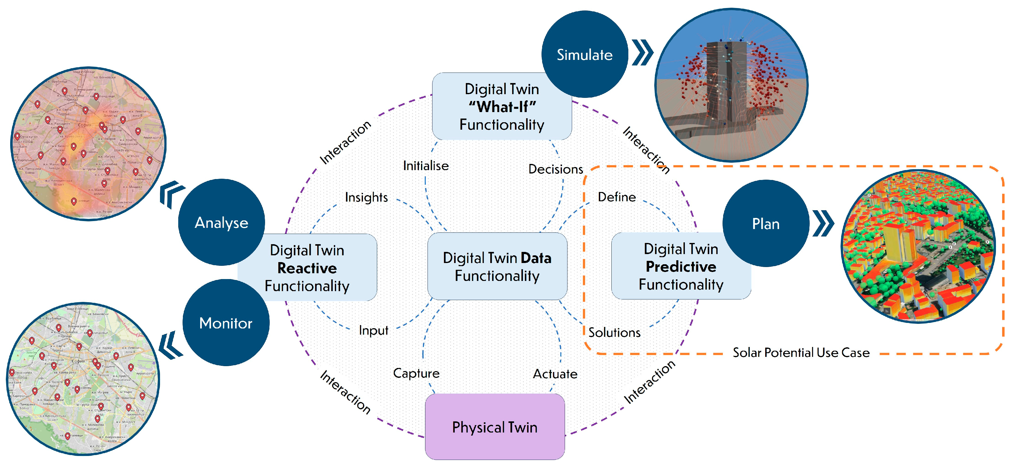
:1. Introduction
2. State-of-the-Art
2.1. Weather Data for Solar Potential
2.2. 3D City Models of Buildings for Solar Potential Studies
2.3. Shading Assessment Using 3D City Models
2.4. Visualisation of Solar Radiation on Building Surfaces
2.5. Software Technologies and Tools
3. Challenges and Gaps
- What kind of geometric preprocessing of terrain data and building footprints is required at the city scale before further analysis in a 3D CAD system?
- Which components of the calculation of solar potential using the CAD-based raytracing method have the most significant impact on computation performance, leading to the improvement of data pipelines for UDTs?
- How can the results of the calculations be visualised on the web at the city scale?
4. Materials and Methods
4.1. Study Area and Data
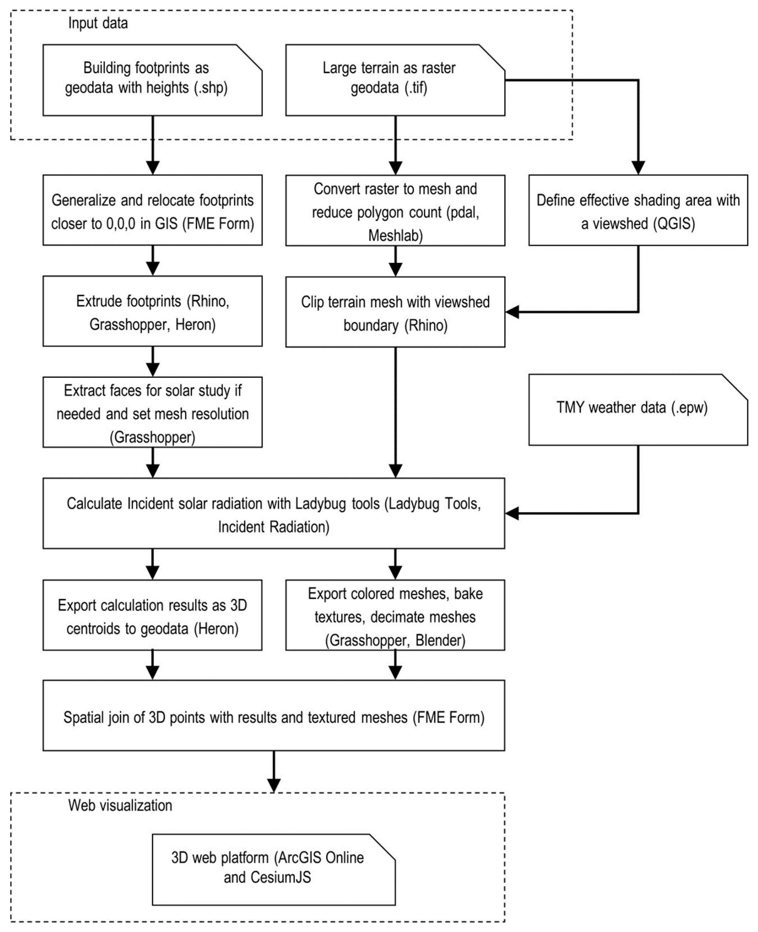
4.2. General Workflow
4.3. Preprocess Geodata and Generation of 3D LOD1 Buildings
4.4. Effective Shading Terrain Surface and 3D Terrain Generation
4.5. Weather Data Acquisition
4.6. Calculating Solar Radiation
4.6.1. Generation of the Cumulative Sky Matrix
4.6.2. Ladybug Incident Radiation
4.6.3. Transferring Results to a 3D Web Platform
5. Results
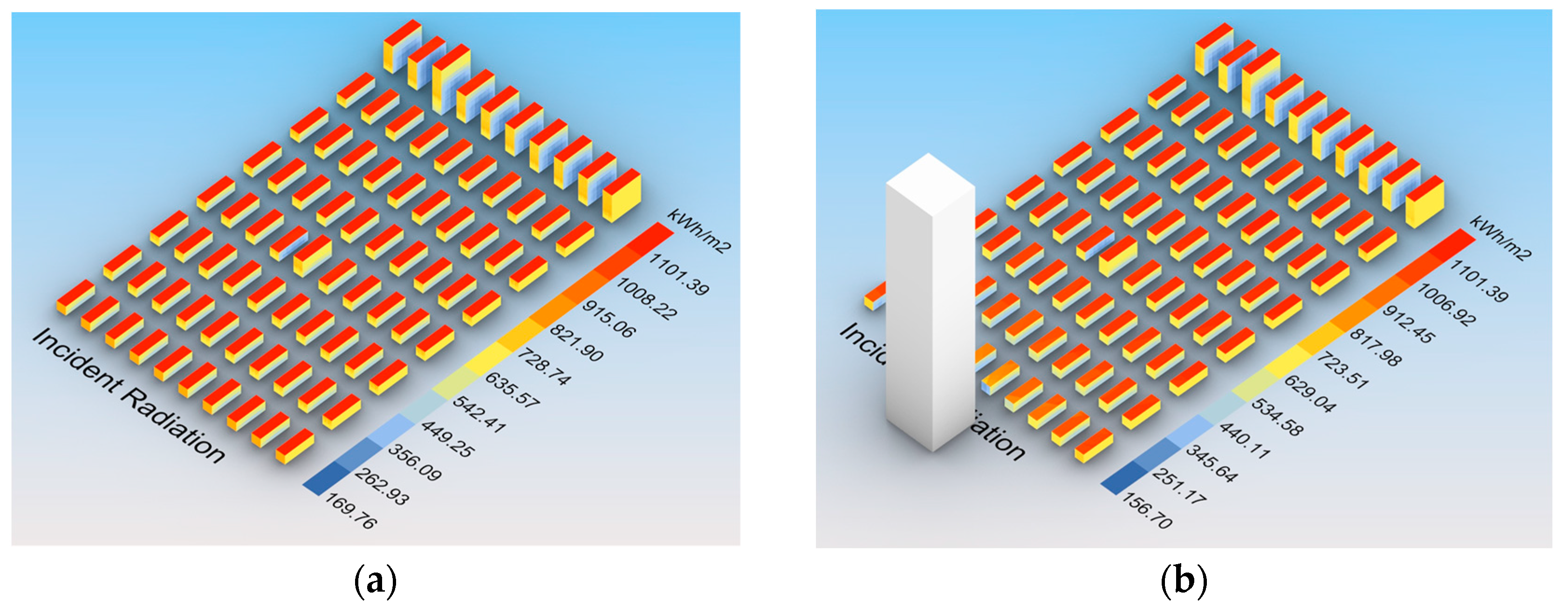
5.1. Impact of Large Distant Shading Objects
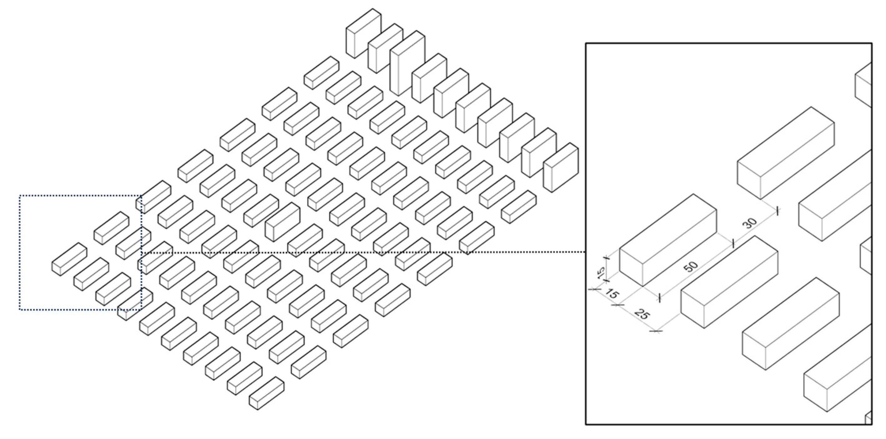
5.2. Synthetic Buildings
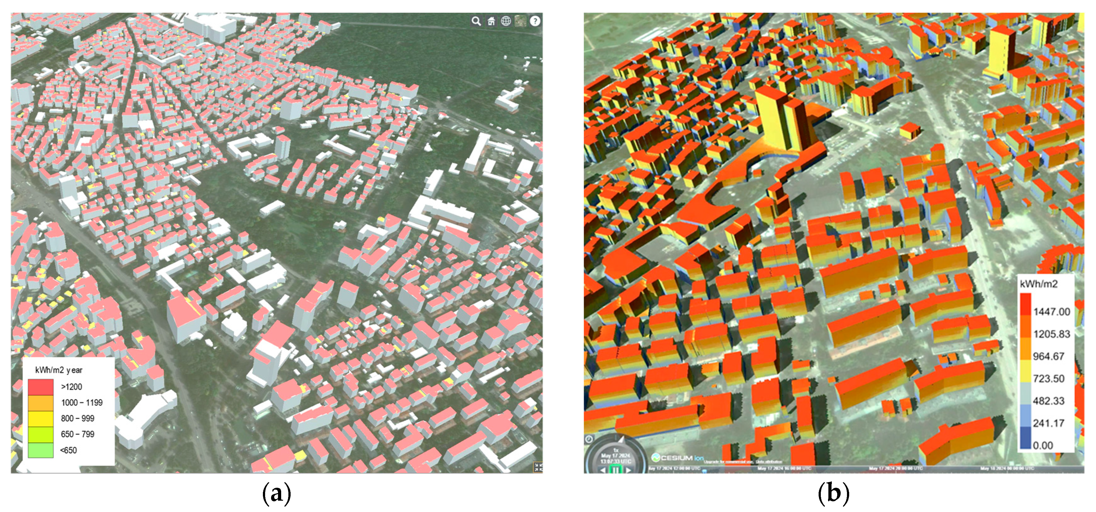
5.3. Case 1. City Scale
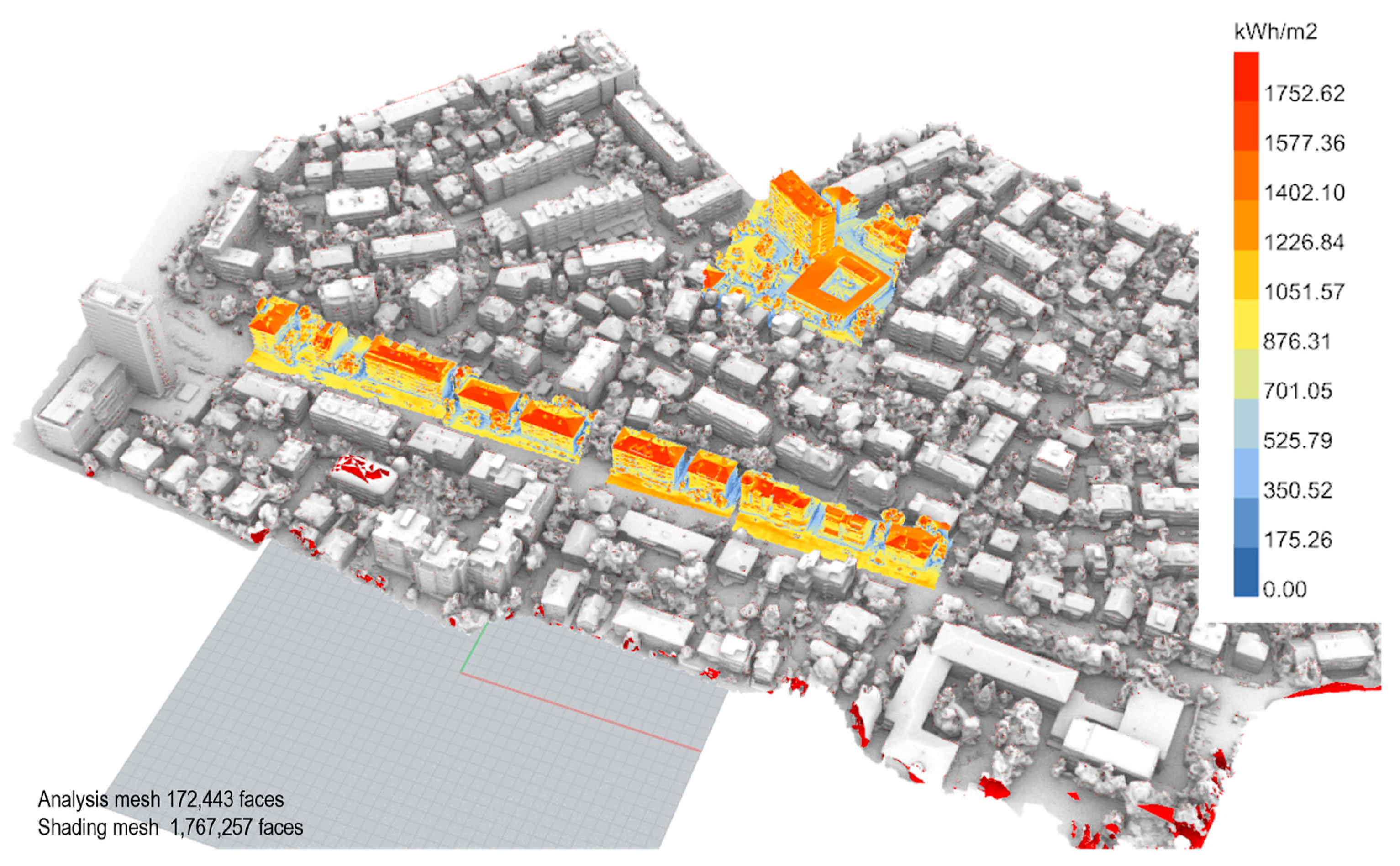
5.4. Case 2. District Scale
6. Discussion
6.1. Use Cases
6.2. Limitations
6.3. Challenges and Gaps
7. Conclusions and Outlook
Author Contributions
Funding
Data Availability Statement
Acknowledgments
Conflicts of Interest
References
- Czachura, A.; Kanters, J.; Gentile, N.; Wall, M. Solar Performance Metrics in Urban Planning: A Review and Taxonomy. Buildings 2022, 12, 393. [Google Scholar] [CrossRef]
- Hasan, J.; Horvat, M. Spatial Parameters and Methodological Approaches in Solar Potential Assessment-State-of-the-Art. Renew. Sustain. Energy Rev. 2023, 188, 113857. [Google Scholar] [CrossRef]
- Suitability of Roofs for the Use of Solar Energy. Available online: https://www.geocat.ch/geonetwork/srv/eng/catalog.search#/metadata/b614de5c-2f12-4355-b2c9-7aef2c363ad6 (accessed on 1 February 2024).
- City of Vienna. Vienna Environmental Good. Available online: https://www.wien.gv.at/umweltgut/public/grafik.aspx?ThemePage=9 (accessed on 1 February 2024).
- JRC Photovoltaic Geographical Information System (PVGIS)-European Commission. Available online: https://re.jrc.ec.europa.eu/pvg_tools/en/ (accessed on 1 February 2024).
- Global Solar Atlas. Available online: https://globalsolaratlas.info/map?c=42.694296,23.586273,11&s=42.688997,23.345947&m=site (accessed on 1 February 2024).
- Google Maps Platform. Solar API Concepts. Available online: https://developers.google.com/maps/documentation/solar/concepts (accessed on 1 February 2024).
- Startira Kandidatstvaneto Na Domakinstvata Za Finansirane Na Fotovoltaichni Sistemi [Household Applications for Photovoltaic Systems Financing Launched]. Available online: https://me.government.bg/themes/startira-kandidatstvaneto-na-domakinstvata-za-finansirane-na-fotovoltaichni-sistemi-2454-1639.html (accessed on 1 February 2024).
- Solar Cities–Project Cities powered by sun. Available online: https://solarcities.bg/ (accessed on 1 February 2024).
- Catita, C.; Redweik, P.; Pereira, J.; Brito, M.C. Extending Solar Potential Analysis in Buildings to Vertical Facades. Comp. Geosci. 2014, 66, 1–12. [Google Scholar] [CrossRef]
- Jaugsch, F.; Löwner, M.-O. Estimation of Solar Energy on Vertical 3d Building Walls on City Quarter Scale. Int. Arch. Photogramm. Remote Sens. Spat. Inf. Sci. 2016, XLII-2-W2, 135–143. [Google Scholar] [CrossRef]
- Saretta, E.; Bonomo, P.; Frontini, F. A Calculation Method for the BIPV Potential of Swiss Façades at LOD2.5 in Urban Areas: A Case from Ticino Region. Sol. Energy 2020, 195, 150–165. [Google Scholar] [CrossRef]
- Manni, M.; Nocente, A.; Kong, G.; Skeie, K.; Fan, H.; Lobaccaro, G. Solar Energy Digitalization at High Latitudes: A Model Chain Combining Solar Irradiation Models, a LiDAR Scanner, and High-Detail 3D Building Model. Front. Energy Res. 2022, 10, 1082092. [Google Scholar] [CrossRef]
- Formolli, M.; Kleiven, T.; Lobaccaro, G. Solar Accessibility at the Neighborhood Scale: A Multi-Domain Analysis to Assess the Impact of Urban Densification in Nordic Built Environments. Sol. Energy Adv. 2022, 2, 100023. [Google Scholar] [CrossRef]
- Biljecki, F.; Stoter, J.; Ledoux, H.; Zlatanova, S.; Çöltekin, A. Applications of 3D City Models: State of the Art Review. ISPRS Int. J. Geo-Inf. 2015, 4, 2842–2889. [Google Scholar] [CrossRef]
- Willenborg, B.; Sindram, M.; Kolbe, T.H. Applications of 3D City Models for a Better Understanding of the Built Environment. In Trends in Spatial Analysis and Modelling: Decision-Support and Planning Strategies; Behnisch, M., Meinel, G., Eds.; Springer International Publishing: Cham, Switzerland, 2018; pp. 167–191. ISBN 978-3-319-52522-8. [Google Scholar]
- Kolečanský, Š.; Hofierka, J.; Bogľarský, J.; Šupinský, J. Comparing 2D and 3D Solar Radiation Modeling in Urban Areas. Energies 2021, 14, 8364. [Google Scholar] [CrossRef]
- Tan, P.Y.; Ismail, M.R.B. The Effects of Urban Forms on Photosynthetically Active Radiation and Urban Greenery in a Compact City. Urban Ecosyst. 2015, 18, 937–961. [Google Scholar] [CrossRef]
- Standards, E. BS EN 17037:2018+A1:2021 Daylight in Buildings. Available online: https://www.en-standard.eu/bs-en-17037-2018-a1-2021-daylight-in-buildings/ (accessed on 27 February 2024).
- Naredba № 7 ot 22 Dekemvri 2003 g. za Pravila i Normativi za Ustroystvo na Otdelnite Vidove Teritorii i Ustroystveni zoni [Ordinance no. 7 of 22 December 2003 on Rules and Codes for the Development of Certain Types of Territories and Development zones]. Available online: https://lex.bg/laws/ldoc/2135476546 (accessed on 1 February 2024).
- Singh, M.; Fuenmayor, E.; Hinchy, E.P.; Qiao, Y.; Murray, N.; Devine, D. Digital Twin: Origin to Future. Appl. Syst. Innov. 2021, 4, 36. [Google Scholar] [CrossRef]
- VanDerHorn, E.; Mahadevan, S. Digital Twin: Generalization, Characterization and Implementation. Decis. Support Syst. 2021, 145, 113524. [Google Scholar] [CrossRef]
- Freitas, S.; Catita, C.; Redweik, P.; Brito, M.C. Modelling Solar Potential in the Urban Environment: State-of-the-Art Review. Renew. Sustain. Energy Rev. 2015, 41, 915–931. [Google Scholar] [CrossRef]
- Yang, D. Solar Radiation on Inclined Surfaces: Corrections and Benchmarks. Sol. Energy 2016, 136, 288–302. [Google Scholar] [CrossRef]
- Šúri, M.; Hofierka, J. A New GIS-Based Solar Radiation Model and Its Application to Photovoltaic Assessments. Trans. GIS 2004, 8, 175–190. [Google Scholar] [CrossRef]
- Fu, P.; Rich, P. Design and Implementation of the Solar Analyst: An ArcView Extension for Modeling Solar Radiation at Landscape Scales. In Proceedings of the IX Annual ESRI User Conference, San Diego, CA, USA, 26–30 July 1991. [Google Scholar]
- Zhao, H.; Yang, R.J.; Liu, C.; Sun, C. Solar Building Envelope Potential in Urban Environments: A State-of-the-Art Review of Assessment Methods and Framework. Build. Environ. 2023, 244, 110831. [Google Scholar] [CrossRef]
- Ni, P.; Yan, Z.; Yue, Y.; Xian, L.; Lei, F.; Yan, X. Simulation of Solar Radiation on Metropolitan Building Surfaces: A Novel and Flexible Research Framework. Sustain. Cities Soc. 2023, 93, 104469. [Google Scholar] [CrossRef]
- Vartholomaios, A. A Machine Learning Approach to Modelling Solar Irradiation of Urban and Terrain 3D Models. Comput. Environ. Urban Syst. 2019, 78, 101387. [Google Scholar] [CrossRef]
- Zhang, Y.; Schlueter, A.; Waibel, C. SolarGAN: Synthetic Annual Solar Irradiance Time Series on Urban Building Facades via Deep Generative Networks. Energy AI 2023, 12, 100223. [Google Scholar] [CrossRef]
- Deep Umbra. Available online: https://www.evl.uic.edu/shadows/ (accessed on 25 February 2024).
- Huld, T.; Paietta, E.; Zangheri, P.; Pinedo Pascua, I. Assembling Typical Meteorological Year Data Sets for Building Energy Performance Using Reanalysis and Satellite-Based Data. Atmosphere 2018, 9, 53. [Google Scholar] [CrossRef]
- PVGIS Data Sources & Calculation Methods-European Commission. Available online: https://joint-research-centre.ec.europa.eu/photovoltaic-geographical-information-system-pvgis/getting-started-pvgis/pvgis-data-sources-calculation-methods_en (accessed on 1 February 2024).
- Climate.Onebuilding.Org. Available online: https://climate.onebuilding.org/ (accessed on 1 February 2024).
- EnergyPlus Weather Data. Available online: https://energyplus.net/weather (accessed on 1 February 2024).
- White Box Technologies. ASHRAE IWEC2 Weather Files. Available online: http://weather.whiteboxtechnologies.com/IWEC2 (accessed on 1 February 2024).
- Meteonorm. TMY3 (NREL & DWD). Available online: https://meteonorm.com/en/typical-meteorological-years (accessed on 1 February 2024).
- Meteonorm Horizon Tiles. Available online: https://meteonorm.com/en/horizon-tiles (accessed on 1 February 2024).
- Ivanova, S. Climate Scenario-Based Design and Construction and Regional Climate Models. In Proceedings of the VIII International Scientific Conference “Industry 4.0”, Winter Session, Borovets, Bulgaria, 6 December 2023; pp. 336–339. [Google Scholar]
- Johari, F.; Peronato, G.; Sadeghian, P.; Zhao, X.; Widén, J. Urban Building Energy Modeling: State of the Art and Future Prospects. Renew. Sustain. Energy Rev. 2020, 128, 109902. [Google Scholar] [CrossRef]
- Willenborg, B.; Pültz, M.; Kolbe, T.H. Integration of Semantic 3d City Models and 3d Mesh Models for Accuracy Improvements of Solar Potential Analyses. Int. Arch. Photogramm. Remote Sens. Spat. Inf. Sci. 2018, XLII-4/W10, 223–230. [Google Scholar] [CrossRef]
- Gröger, G.; Plümer, L. CityGML–Interoperable Semantic 3D City Models. ISPRS J. Photogramm. Remote Sens. 2012, 71, 12–33. [Google Scholar] [CrossRef]
- Pađen, I.; García-Sánchez, C.; Ledoux, H. Towards Automatic Reconstruction of 3D City Models Tailored for Urban Flow Simulations. Front. Built Environ. 2022, 8, 899332. [Google Scholar] [CrossRef]
- Peronato, G.; Rey, E.; Andersen, M. 3D Model Discretization in Assessing Urban Solar Potential: The Effect of Grid Spacing on Predicted Solar Irradiation. Sol. Energy 2018, 176, 334–349. [Google Scholar] [CrossRef]
- Biljecki, F.; Ledoux, H.; Stoter, J. Does a Finer Level of Detail of a 3D City Model Bring an Improvement for Estimating Shadows. In Advances in 3D Geoinformation; Abdul-Rahman, A., Ed.; Springer International Publishing: Cham, Switzerland, 2017; pp. 31–47. ISBN 978-3-319-25691-7. [Google Scholar]
- Biljecki, F.; Ledoux, H.; Stoter, J.; Vosselman, G. The Variants of an LOD of a 3D Building Model and Their Influence on Spatial Analyses. ISPRS J. Photogramm. Remote Sens. 2016, 116, 42–54. [Google Scholar] [CrossRef]
- Alam, N.; Coors, V.; Zlatanova, S.; Oosterom, P.J.M. Shadow Effect on Photovoltaic Potentiality Analysis Using 3D City Models. Int. Arch. Photogramm. Remote Sens. Spat. Inf. Sci. 2012, XXXIX-B8, 209–214. [Google Scholar] [CrossRef]
- Peronato, G.; Rastogi, P.; Rey, E.; Andersen, M. A Toolkit for Multi-Scale Mapping of the Solar Energy-Generation Potential of Buildings in Urban Environments under Uncertainty. Sol. Energy 2018, 173, 861–874. [Google Scholar] [CrossRef]
- Marsh, A. The Application of Shading Masks in Building Simulation. In Proceedings of the International IBPSA Conference: Building Simulation 2005, Montréal, QC, Canada, 15 August 2005; pp. 725–732. [Google Scholar]
- Chatzipoulka, C.; Compagnon, R.; Kaempf, J.; Nikolopoulou, M. Sky View Factor as Predictor of Solar Availability on Building Façades. Sol. Energy 2018, 170, 1026–1038. [Google Scholar] [CrossRef]
- Robinson, D.; Stone, A. A Simplified Radiosity Algorithm for General Urban Radiation Exchange. Build. Serv. Eng. Res. Technol. 2005, 26, 271–284. [Google Scholar] [CrossRef]
- Radiance. A Validated Lighting Simulation Tool. Available online: https://www.radiance-online.org/ (accessed on 1 February 2024).
- Jakubiec, J.A.; Reinhart, C.F. A Method for Predicting City-Wide Electricity Gains from Photovoltaic Panels Based on LiDAR and GIS Data Combined with Hourly Daysim Simulations. Sol. Energy 2013, 93, 127–143. [Google Scholar] [CrossRef]
- Bremer, M.; Mayr, A.; Wichmann, V.; Schmidtner, K.; Rutzinger, M. A New Multi-Scale 3D-GIS-Approach for the Assessment and Dissemination of Solar Income of Digital City Models. Comput. Environ. Urban. Syst. 2016, 57, 144–154. [Google Scholar] [CrossRef]
- Spasic, D. Gismo 2024. Available online: https://github.com/stgeorges/gismo (accessed on 1 February 2024).
- Horizon Profile-European Commission. Available online: https://joint-research-centre.ec.europa.eu/photovoltaic-geographical-information-system-pvgis/pvgis-tools/horizon-profile_en (accessed on 1 February 2024).
- CitySIM Pro. Frequently Asked Questions (FAQ). Available online: http://www.kaemco.ch/download.php (accessed on 1 February 2024).
- Alam, N.; Coors, V.; Zlatanova, S.; Oosterom, P.J.M. Resolution in Photovoltaic Potential Computation. ISPRS Ann. Photogramm. Remote Sens. Spat. Inf. Sci. 2016, IV-4/W1, 89–96. [Google Scholar] [CrossRef]
- Perez, R.; Seals, R.; Michalsky, J. All-Weather Model for Sky Luminance Distribution—Preliminary Configuration and Validation. Sol. Energy 1993, 50, 235–245. [Google Scholar] [CrossRef]
- Subramaniam, S.; Mistrick, R.G. A More Accurate Approach for Calculating Illuminance with Daylight Coefficients. In Proceedings of the 2017 Annual IES Conference, Portland, OR, USA, 8–10 August 2017. [Google Scholar]
- Sadeghipour Roudsari, M.; Pak, M. Ladybug: A Parametric Environmental Plugin for Grasshopper to Help Designers Create an Environmentally-Conscious Design. In Proceedings of the BS 2013: 13th Conference of the International Building Performance Simulation Association, Chambery, France, 25–28 August 2013; pp. 3128–3135. [Google Scholar]
- Liao, W.; Heo, Y.; Xu, S. Simplified Vector-Based Model Tailored for Urban-Scale Prediction of Solar Irradiance. Sol. Energy 2019, 183, 566–586. [Google Scholar] [CrossRef]
- Beran, D.; Jedlička, K.; Kumar, K.; Popelka, S.; Stoter, J. The Third Dimension in Noise Visualization–a Design of New Methods for Continuous Phenomenon Visualization. Cartogr. J. 2022, 59, 1–17. [Google Scholar] [CrossRef]
- Moreira, G.; Hosseini, M.; Alam Nipu, M.N.; Lage, M.; Ferreira, N.; Miranda, F. The Urban Toolkit: A Grammar-Based Framework for Urban Visual Analytics. IEEE Trans. Vis. Comput. Graph. 2024, 30, 1402–1412. [Google Scholar] [CrossRef]
- Mota, R.; Ferreira, N.; Silva, J.D.; Horga, M.; Lage, M.; Ceferino, L.; Alim, U.; Sharlin, E.; Miranda, F. A Comparison of Spatiotemporal Visualizations for 3D Urban Analytics. IEEE Trans. Vis. Comput. Graph. 2023, 29, 1277–1287. [Google Scholar] [CrossRef]
- Chaturvedi, K.; Willenborg, B.; Sindram, M.; Kolbe, T.H. Solar Potential Analysis and Integration of the Time-Dependent Simulation Results for Semantic 3D City Models Using Dynamizers. ISPRS Ann. Photogramm. Remote Sens. Spat. Inf. Sci. 2017, IV-4/W5, 25–32. [Google Scholar] [CrossRef]
- Helsinki. Solar Energy Potential. Available online: https://kartta.hel.fi/3d/solar/#/ (accessed on 1 February 2024).
- City of Bremen. Solar Potential. Available online: https://bremen.virtualcitymap.de/?lang=de&layerToActivate=%5B%22Solar%20Surfaces%22%5D&layerToDeactivate=%5B%22Bremen%20texturiert%22%5D&startingmap=Cesium%20Map&cameraPosition=8.79362%2C53.07704%2C476.20705&groundPosition=8.80659%2C53.07690%2C10.38654&distance=986.13&pitch=-28.19&heading=91.06&roll=0.21#/ (accessed on 3 February 2024).
- Sosa-Tinoco, I.; Prósper, M.A.; Miguez-Macho, G. Development of a Solar Energy Forecasting System for Two Real Solar Plants Based on WRF Solar with Aerosol Input and a Solar Plant Model. Sol. Energy 2022, 240, 329–341. [Google Scholar] [CrossRef]
- Autodesk Revit 2023. Help|about Solar Analysis|Autodesk. Available online: https://help.autodesk.com/view/RVT/2023/ENU/?guid=GUID-15701517-EB11-460D-9BC9-EDEC7AE68BB9 (accessed on 1 February 2024).
- Brito, M.C.; Redweik, P.; Catita, C.; Freitas, S.; Santos, M. 3D Solar Potential in the Urban Environment: A Case Study in Lisbon. Energies 2019, 12, 3457. [Google Scholar] [CrossRef]
- Zahn, W. Sonneneinstrahlungsanalyse auf und Informationsanreicherung von großen 3D-Stadtmodellen im CityGML-Schema. Master’s Thesis, Technische Universität München, München, Germany, 2015. [Google Scholar]
- Braun, C. A Scalable Approach for Spatio-Temporal Assessment of Photovoltaic Electricity Potentials for Building Façades of Entire Cities. Int. Arch. Photogramm. Remote Sens. Spat. Inf. Sci. 2019, XLII-4/W14, 17–22. [Google Scholar] [CrossRef]
- Jakica, N. State-of-the-Art Review of Solar Design Tools and Methods for Assessing Daylighting and Solar Potential for Building-Integrated Photovoltaics. Renew. Sustain. Energy Rev. 2018, 81, 1296–1328. [Google Scholar] [CrossRef]
- Giannelli, D.; León-Sánchez, C.; Agugiaro, G. Comparison and Evaluation of Different GIS Software Tools to Estimate Solar Irradiation. Int. Arch. Photogramm. Remote Sens. Spat. Inf. Sci. 2022, V-4–2022, 275–282. [Google Scholar] [CrossRef]
- SimStadt Documentation. Available online: https://simstadt.hft-stuttgart.de/ (accessed on 4 February 2024).
- Thebault, M.; Govehovitch, B.; Bouty, K.; Caliot, C.; Compagnon, R.; Desthieux, G.; Formolli, M.; Giroux-Julien, S.; Guillot, V.; Herman, E.; et al. A Comparative Study of Simulation Tools to Model the Solar Irradiation on Building Façades. In Proceedings of the ISES SWC 2021 Solar World Congress, Virtual Conference, 25–29 October 2021; p. 12. [Google Scholar] [CrossRef]
- Rodríguez, L.R.; Nouvel, R.; Duminil, E.; Eicker, U. Setting Intelligent City Tiling Strategies for Urban Shading Simulations. Sol. Energy 2017, 157, 880–894. [Google Scholar] [CrossRef]
- Vo, A.V.; Laefer, D.F.; Smolic, A.; Zolanvari, S.M.I. Per-Point Processing for Detailed Urban Solar Estimation with Aerial Laser Scanning and Distributed Computing. ISPRS J. Photogramm. Remote Sens. 2019, 155, 119–135. [Google Scholar] [CrossRef]
- Associates, R.M. How Accurate Is Rhino? Available online: https://www.rhino3d.com/features/accuracy/ (accessed on 1 February 2024).
- Naserentin, V.; Somanath, S.; Eleftheriou, O.; Logg, A. Combining Open Source and Commercial Tools in Digital Twin for Cities Generation. IFAC-Pap. 2022, 55, 185–189. [Google Scholar] [CrossRef]
- Piepereit, R.; Deininger, M.; Kada, M.; Pries, M.; Voß, U. A Sweep-Plane Algorithm For The Simplification Of 3d Building Models In The Application Scenario Of Wind Simulations. Int. Arch. Photogramm. Remote Sens. Spat. Inf. Sci. 2018, XLII-4/W10, 151–156. [Google Scholar] [CrossRef]
- Azeez, A. Realize the Potential of Forma’s Solar Energy Analysis. Available online: https://blogs.autodesk.com/forma/2023/10/12/realize-the-potential-of-formas-solar-energy-analysis/ (accessed on 4 February 2024).
- de Sousa Freitas, J.; Cronemberger, J.; Soares, R.M.; Amorim, C.N.D. Modeling and Assessing BIPV Envelopes Using Parametric Rhinoceros Plugins Grasshopper and Ladybug. Renew. Energy 2020, 160, 1468–1479. [Google Scholar] [CrossRef]
- Poon, K.H.; Kämpf, J.H.; Tay, S.E.R.; Wong, N.H.; Reindl, T.G. Parametric Study of URBAN Morphology on Building Solar Energy Potential in Singapore Context. Urban Clim. 2020, 33, 100624. [Google Scholar] [CrossRef]
- Zhu, D.; Song, D.; Shi, J.; Fang, J.; Zhou, Y. The Effect of Morphology on Solar Potential of High-Density Residential Area: A Case Study of Shanghai. Energies 2020, 13, 2215. [Google Scholar] [CrossRef]
- Xia, B.; Li, Z. Optimized Methods for Morphological Design of Mesoscale Cities Based on Performance Analysis: Taking the Residential Urban Blocks as Examples. Sustain. Cities Soc. 2021, 64, 102489. [Google Scholar] [CrossRef]
- Sustainable Energy and Climate Action Plan of Sofia Municipality 2021–2030 Including Energy Efficiency Programme and Long-Term Programme to Promote the Use of Renewable Energy and Bio-Fuels. Available online: https://www.sofia.bg/climat (accessed on 1 February 2024).
- Washburn, B. Heron: An Add-on for Grasshopper Enabling the GIS Functions of GDAL in Rhino 3d 2024. Available online: https://github.com/blueherongis/Heron (accessed on 20 February 2024).
- BoundingBoxReplacer. Available online: https://docs.safe.com/fme/html/FME-Form-Documentation/FME-Transformers/Transformers/boundingboxreplacer.htm (accessed on 20 February 2024).
- Douglas, D.H.; Peucker, T.K. Algorithms for the Reduction of the Number of Points Required to Represent a Digitized Line or Its Caricature. Cartogr. Int. J. Geogr. Inf. Geovisualization 1973, 10, 112–122. [Google Scholar] [CrossRef]
- LB View Percent-Sky View Factor-Error: “Input Must Be of Type of Color”-Grasshopper/Ladybug. Available online: https://discourse.ladybug.tools/t/lb-view-percent-sky-view-factor-error-input-must-be-of-type-of-color/17797/6 (accessed on 4 February 2024).
- Biljecki, F.; Ledoux, H.; Stoter, J. An Improved LOD Specification for 3D Building Models. Comput. Environ. Urban Syst. 2016, 59, 25–37. [Google Scholar] [CrossRef]
- Čučković, Z. QGIS Visibility Analysis. Available online: https://landscapearchaeology.org/qgis-visibility-analysis/ (accessed on 4 February 2024).
- Ivanova, S. Maximum Summer Values of Solar Irradiation on Horizontal and Vertical Building Surfaces. In Proceedings of the XVI International Scientific Conference VSU’2016, Sofia, Bulgaria, 9–10 June 2016. [Google Scholar]
- Ivanova, S. Analysis of the Necessity for Updates of Solar Data in Ordinance No 7 on Energy Efficiency of Buildings. In Proceedings of the IXth International Scientific Conference on Architecture and Civil Engineering ArCivE Varna, Varna, Bulgaria, 31 May–2 June 2019; Volume I. [Google Scholar]
- Ivanova, S.; Chobanov, P. Modeling the Balance between Solar Heat Gains and Conductive Heat Losses through Building Glass during the Coolest Winter Month in nZEB. In Proceedings of the Conference: V International Scientific Conference “High technologies”, Borovets, Bulgaria, 9 March 2020. [Google Scholar]
- Global Solar Atlas-Site Info. Sredets. Available online: https://globalsolaratlas.info/detail?c=42.647344,23.37719,11&s=42.684454,23.339081&m=site (accessed on 7 February 2024).
- Cumulative Sky Matrix-Ladybug Primer. Available online: https://docs.ladybug.tools/ladybug-primer/components/2_visualizedata/cumulative_sky_matrix (accessed on 4 February 2024).
- Ivanova, S.M.; Gueymard, C.A. Simulation and Applications of Cumulative Anisotropic Sky Radiance Patterns. Sol. Energy 2019, 178, 278–294. [Google Scholar] [CrossRef]
- Incident Radiation. Available online: https://docs.ladybug.tools/ladybug-primer/components/3_analyzegeometry/incident_radiation (accessed on 27 February 2024).


| Total kWh, y | Shading from the Terrain | Percentage | |
|---|---|---|---|
| Building 1 | 145,570.0877 | no | 100.0% |
| Building 1 | 141,928.7915 | yes | 97.5% |
| Building 2 | 145,456.3552 | yes | 99.9% |
| Total kWh, y | Shading from SW | Percentage | |
|---|---|---|---|
| Building 1 | 231,873.0974 | no | 100.00% |
| Building 1 | 195,235.4617 | yes | 84.20% |
| Building 2 | 221,454.6975 | yes | 95.51% |
| Cell Size, m | Face Count | Tr, s | Tr, Shading, s | R, s | R, Graft, s |
|---|---|---|---|---|---|
| 3 | 35,931 | 22.5 | 22.6 | 84 | 84 |
| 2 | 78,806 | 30 | 49.6 | 180 | 186 |
| 1 | 321,574 | 198 | 198 | 840 | 804 |
| 0.75 | 568,692 | 372 | 354 | 2400 | 2016 |
| 0.5 | 1,286,308 | 798 | 834 | - | - |
| 0.4 | 1,988,897 | 1572 | 1960 | - | - |
| 0.25 | 5,146,622 | 33,480 | - | - | - |
| Study Area, km2 | Face Count | Time, s | Ratio Face Count/s | |
|---|---|---|---|---|
| Synthetic buildings | 0.23 | 1,988,897 | 1572 | 1265.2 |
| Case 1 | 315.6 | 1,909,499 | 1926 | 991.4 |
| Case 2 | 13.74 | 1,008,585 | 684 | 1474.6 |
Disclaimer/Publisher’s Note: The statements, opinions and data contained in all publications are solely those of the individual author(s) and contributor(s) and not of MDPI and/or the editor(s). MDPI and/or the editor(s) disclaim responsibility for any injury to people or property resulting from any ideas, methods, instructions or products referred to in the content. |
© 2024 by the authors. Licensee MDPI, Basel, Switzerland. This article is an open access article distributed under the terms and conditions of the Creative Commons Attribution (CC BY) license (https://creativecommons.org/licenses/by/4.0/).
Share and Cite
Shirinyan, E.; Petrova-Antonova, D. Large-Scale Solar Potential Analysis in a 3D CAD Framework as a Use Case of Urban Digital Twins. Remote Sens. 2024, 16, 2700. https://doi.org/10.3390/rs16152700
Shirinyan E, Petrova-Antonova D. Large-Scale Solar Potential Analysis in a 3D CAD Framework as a Use Case of Urban Digital Twins. Remote Sensing. 2024; 16(15):2700. https://doi.org/10.3390/rs16152700
Chicago/Turabian StyleShirinyan, Evgeny, and Dessislava Petrova-Antonova. 2024. "Large-Scale Solar Potential Analysis in a 3D CAD Framework as a Use Case of Urban Digital Twins" Remote Sensing 16, no. 15: 2700. https://doi.org/10.3390/rs16152700