Article

Seasonal Variability in the Relationship between the Volume-Scattering Function at 180° and the Backscattering Coefficient Observed from Spaceborne Lidar and Biogeochemical Argo (BGC-Argo) Floats

1
Southern Marine Science and Engineering Guangdong Laboratory (Guangzhou), No. 1119, Haibin Rd., Nansha District, Guangzhou 511458, China
2
State Key Laboratory of Satellite Ocean Environment Dynamics, Second Institute of Oceanography, Ministry of Natural Resources, 36 Bochubeilu, Hangzhou 310012, China
3
Institute of Oceanographic Instrumentation, Qilu University of Technology (Shandong Academy of Sciences), 37 Miaoling Road, Qingdao 266061, China
4
Donghai Laboratory, No. 1, Zhejiang Da Rd., Dinghai District, Zhoushan 310030, China
*
Author to whom correspondence should be addressed.
Remote Sens. 2024, 16(15), 2704; https://doi.org/10.3390/rs16152704
Submission received: 12 June 2024 / Revised: 12 July 2024 / Accepted: 21 July 2024 / Published: 24 July 2024
(This article belongs to the Section Environmental Remote Sensing)

Abstract

:
The derivation of the particulate-backscattering coefficient (bbp) from Lidar signals is highly influenced by the parameter χp(π), which is defined by χp(π) = bbp/(2πβp(π)). This parameter facilitates the correlation of the particulate-volume-scattering function at 180°, denoted βp(π), with bbp. However, studies exploring the global and seasonal fluctuations of χp(π) remain sparse, largely due to measurement difficulties of βp(π) in the field conditions. This study pioneers the global data collection for χp(π), integrating bbp observations from Biogeochemical Argo (BGC-Argo) floats and βp(π) data from the Cloud-Aerosol Lidar with Orthogonal Polarization (CALIOP) spaceborne lidar. Our findings indicate that χp(π) experiences significant seasonal differences globally, peaking during summer and nadiring in winter. The global average χp(π) was calculated as 0.40, 0.48, 0.43, and 0.35 during spring, summer, autumn, and winter, respectively. The daytime values of χp(π) slightly exceeded those registered at night. To illuminate the seasonal variations in χp(π) in 26 sea regions worldwide, we deployed passive ocean color data MODIS bbp and active remote sensing data CALIOP βp(π), distinguishing three primary seasonal change patterns—the “summer peak”, the “decline”, and the “autumn pole”—with the “summer peak” typology being the most common. Post recalibration of the CALIOP bbp product considering seasonal χp(π) variations, we observed substantial statistical improvements. Specifically, the coefficient of determination (R2) markedly improved from 0.84 to 0.89, while the root mean square error (RMSE) declined from 4.0 × 10⁻⁴ m−1 to 3.0 × 10⁻⁴ m−1. Concurrently, the mean absolute percentage error (MAPE) also dropped significantly, from 31.48% to 25.27%.

1. Introduction

When incident light interacts with a particle, it experiences omnidirectional scattering. The precise characterization of light intensity scattered across diverse scattering angles is encapsulated within the volume-scattering function (VSF), denoted as β(θ) with units of m−1 sr−1 [1,2,3]. The VSF’s relative magnitude, spectral attributes, and angular distribution fundamentally hinge upon the particle’s parameters, including concentration, size, composition, and morphology. Scattering sensors exploit these VSF properties by monitoring precise spectral and angular domains, thereby inferring information about particles [4,5,6,7]. Typically, for the backward portion of VSF with scattering angles (θ) ranging from 90° to 180°, quantification is performed using two variables: the total backscattering coefficient (bb; m−1) and the χp(θ) factor: χ p ( θ ) = b bp 2 π β p ( θ ) . Particulate backscattering coefficients (bbp(θ)), a core parameter in ocean optics that are applied in marine ecology and biogeochemistry studies [8,9,10], can be determined through estimation from the measurement of βp(θ) using an χp(θ) factor [11].
Particulate backscattering coefficients (bbp) are typically determined through in situ methodologies or passive satellite remote sensing of ocean color. The former approach mandates the installation of measurement instruments on vessels or buoys, necessitating substantial expenditures of human labor, resources, and financial resources for on-site data acquisition. Furthermore, it is unsuitable for expeditious large-scale evaluations, thereby imposing constraints on comprehensive global marine investigations [12,13]. Passive satellite remote sensing of ocean color has offered a continuous record of global surface water properties for over two decades. Nevertheless, this approach, reliant on natural light, inherently harbors certain limitations. It is unsuitable for nighttime observations, periods characterized by dense cloud cover, and high-latitude polar regions [14]. In contrast, spaceborne lidar technology possesses the potential to overcome these constraints. By utilizing emitted pulsed laser systems for aquatic data acquisition, it operates independently of solar illumination, thus enabling the study of variations between day and night in the characteristics of planktonic organisms and facilitating continuous observations during polar night periods [15,16].
Lidar echoes encompass two fundamental properties of seawater: the volume-scattering function at a scattering angle of 180° (β(π); m−1 sr−1) and the lidar attenuation coefficient (α) [17,18]. The particulate backscattering coefficient (bbp) can be obtained through inversion by converting the measured β(π) from spaceborne lidar, but there is some uncertainty in the conversion factor χp(π) within the inversion model. Previous investigations scrutinizing the precision of Cloud-Aerosol Lidar with Orthogonal Polarization (CALIOP) bbp products have disclosed that modifications to the conversion factor exert a substantial influence on the data quality. For instance, Bisson et al. achieved distinct evaluation outcomes, compared to Lacour, by dividing the conversion factor by 2 [19,20,21,22]. Furthermore, it should be noted that the magnitude of χp(π) is profoundly governed by the morphology and internal constitution of particles. Adopting a uniform value of χp(π) for the interpretation of lidar signals obtained from varied aquatic environments may engender considerable inaccuracies [23]. Hair et al. conducted measurements of βp(π) in open waters proximate to the Gulf of Maine, Bermuda, and the coastal regions spanning from Virginia to Rhode Island, employing High Spectral Resolution Lidar (HSRL). Concurrently, they ascertained bbp in these aqueous domains utilizing the ECO-BB3 sensor, with the resultant mean value of χp(π) approximating 0.5 [24]. In other studies [2,25], χp(π) values were reported as 1.43, while in some studies [26,27,28], χp(π) values were reported as 1.06. Zhang et al. identified notable variations in χp data procured in proximity to Ocean Station Papa (50°N 145°W) in contrast to data gathered from multiple global oceanic regions [29]. Consequently, the exploration of seasonal disparities in χp(π) and the establishment of optimal reference values for the conversion factor during distinct seasons assume paramount importance in the pursuit of enhanced accuracy in the inversion of CALIOP bbp products.
Nevertheless, due to the contamination of stray light from reflections, measurements of VSF at angles greater than 173° are not reliable, as they can lead to spurious increases in the scattering of the reflection angle [30,31,32]. Field measurements of the particle volume-scattering function (VSF) at 180° pose certain difficulties, resulting in a limited understanding of the natural variations in χp(π) [2,33]. Thus, we employ in situ bbp measurements collected by Biogeochemical Argo (BGC-Argo) floats to rectify CALIOP’s inverted bbp products, obtaining calibrated values for the corresponding conversion coefficient χp(π). Additionally, we utilize passive ocean-color-remote-sensing data product MODIS bbp to address the spatial limitations in the global coverage of BGC-Argo, resulting in the acquisition of calibrated values for the conversion coefficient χp(π) across diverse oceanic regions.
In this study, based on BGC-Argo and MODIS bbp data, we investigated the seasonal variability of the conversion coefficient χp(π) between the globally observed volume-scattering function at 180° from spaceborne lidar and the particulate-backscattering coefficient. Initially, we established 12 spatiotemporal windows for matching. Utilizing BGC-Argo bbp as in situ data, we calibrated CALIOP bbp, obtaining reference values of χp(π) at different spatiotemporal scales. We conducted a comprehensive examination and comparison of the seasonal changes in χp(π) (refer to Section 3.1), as well as fluctuations between day and night (consult Section 3.2). Subsequently, using the average calibrated χp(π) values from all spatiotemporal windows, we corrected the CALIOP bbp data. An assessment and comparative analysis of the bbp products’ efficacy both pre-correction and post-correction is presented in Section 3.3. Furthermore, a discussion on the influence of band conversion coefficients on χp(π) can be found in Section 4.1. In addition, the effect of atmospheric turbulence can be found in Section 4.2. Finally, to tackle the limited availability of BGC-Argo float measurements in specific marine regions, exploration and analysis of the seasonal oscillations in χp(π) within distinct oceanic domains were performed. This was facilitated through the utilization of the passive ocean-color-remote-sensing product, enabling an investigation into the seasonal trends of χp(π) across diverse global regions, as detailed in Section 4.3.

2. Materials and Methods

2.1. BGC-Argo bbp(700)

The sensors used to measure backscattering at 700 nm on the BGC-Argo float include the ECO Triplet water-color measurement instrument, the Eco-FLBB fluorescence and backscattering meter from WET Labs, and the MCOMS from Seabird, with angles of 124°, 142°, and 149°, respectively [34,35]. After subtracting the contribution of pure seawater, the particulate-backscattering coefficient at 700 nm, bbp(700), is derived [11,36,37]. The data vertical resolution is 1 m between 10 and 250 m, and 0.20 m between 10 m and the sea surface [38].
In this investigation, we employed BGC-Argo float data made available by IFREMER (ftp://ftp.ifremer.fr/ifremer/argo/ (accessed on 9 June 2022)) (Table 1). The dataset encompasses 43,073 vertical profiles of bbp(700 nm; m−1), spanning from January 2010 to April 2017, and boasts comprehensive global coverage, even extending into polar regions. This dataset serves as a valuable resource for the calibration and validation of worldwide satellite-based lidar ocean-profile-remote-sensing products.
To ensure the precision and validity of the collected data, we diligently adhered to the technical guidelines provided by WETLabs (2016) and implemented the real-time quality control methodology introduced by Giorgio Dall’Olmo and colleagues [39]. The vertical profiles of bbp(700) underwent quality control tests for missing data, high outliers, negative values, noise profiles, and mooring spikes, while negative peaks were also eliminated [40] (Figure 1).
After quality control, we identified a total of 1012 float points that did not pass the tests, representing 2.35% of all floats, as shown in Figure 1b. These points are primarily distributed in coastal waters and the Southern Ocean, as depicted in Figure 1a. Upon further inspection, we determined that 237 of these points were bad data which failed the missing data test, negative values test, and mooring spikes (marked with a quality control factor of 4) accounting for 0.55% of all floats, mainly found in the coastal waters of the Indian Ocean and the Southern Ocean. Additionally, we identified 757 potentially invalid data profiles (marked with a quality control factor of 2), constituting 1.76% of all floats, primarily distributed in the Indian Ocean, the Southern Ocean, and the coastal waters of Australia. The quality control tests also revealed 18 missing data float points (marked with a quality control factor of 3), accounting for 0.04% of all floats, mainly located in the Arabian Sea and the Bay of Bengal.
After removing these non-compliant float points, we applied a three-point moving median method to eliminate outliers (values beyond 1.5 times the interquartile range) from the high-quality float bbp(700) profiles. Ultimately, we used 42,061 profiles marked as high-quality vertical observation profiles for the calculation of the conversion factor χp(π) and the calibration of CALIOP product performance.

2.2. MODIS bbp(700)

The retrieval of the ocean water backscattering coefficient (bbp(λ)) is a complex problem that requires the use of spectral remote sensing reflectance (Rrs(λ); sr−1) as input and is subject to a series of assumptions and constraints regarding the absorption and backscattering components in the ocean. Bisson et al. (2019) demonstrated in their study that the performance of the MODIS satellite in global ocean-color-remote-sensing is superior to other contemporary satellites such as the Visible Infrared Imaging Radiometer Suite (VIIRS) and the Ocean and Land Color Instrument (OLCI) [20]. Based on this, we selected bbp(443) derived from MODIS Aqua as the water-color-remote-sensing data. We conducted a spatial–temporal match with BGC-Argo float bbp within a 9 km spatial window and a 12 h temporal window to study regional differences in the conversion factor χp(π). The MODIS data product bbp(443) used in this study was obtained from the Ocean Color website (https://search.earthdata.nasa.gov/ (accessed on 9 June 2022)) (Table 1). Its temporal resolution is a day, spatial resolution is 9 km, and it has been radiometrically calibrated and atmospherically corrected.
To compare with the validation and evaluation of CALIOP bbp(532), we first performed a band conversion on MODIS bbp(443). The conversion to bbp(532) was conducted using the following band conversion formula:
b bp ( 532 ) = b bp ( 443 ) ( 443 532 ) γ
The power–law slope (γ) used in the conversion is 0.78 [41]. Then, the 3σ principle was used to remove outliers from the MODIS bbp data, following the formula:
| x i x ¯ | > 3 ( x 1 x ¯ ) 2 + ( x 2 x ¯ ) 2 + + ( x n x ¯ ) 2 n 1
where xi represents the observed bbp values from MODIS.
The specific elimination process involves the following: firstly, calculating the standard deviation; secondly, computing the absolute difference between each sample point and the mean, comparing it with three times the standard deviation, and if it exceeds three times the standard deviation, it is removed; thirdly, repeating steps 1 until no further removals occur in this iteration. After removing outliers using the 3σ rule, it was found that the overall MODIS bbp is 1.56 times larger than BGC-Argo bbp. Therefore, based on this factor, an offset correction is applied, ensuring the accuracy of MODIS bbp and enabling the study of the global conversion factor χp(π).

2.3. CALIOP β(π)

The Cloud-Aerosol Lidar and Infrared Pathfinder Satellite Observation (CALIPSO) satellite, launched in 2006, is equipped with the CALIOP lidar system, capable of emitting laser pulses at both 1064 nm and 532 nm wavelengths. Notably, the 532 nm channel incorporates dual-polarization features, comprising cross-polarized and co-polarized channels [15]. The parallel channel signals in CALIOP are influenced by molecular scattering, while the cross-polarized channel is mainly caused by the backscattering of particles. The off-nadir tilt enhances the polarization ratio of particles, and it was compared with the diffuse attenuation coefficient (Kd, 532 nm) obtained from airborne lidar, with an average Kd of 1.76 [10,42]. Using these empirical linear relationships between the polarization ratio and Kd, the particle polarization ratio and Kd cancel each other out in the equation.
Due to the negligible contribution of sea surface reflection, the vertically polarized component of the water column integrated attenuated backscatter, βw+, is calculated using the following:
β w + = δ T ( β w / + β s )
where δT represents the ratio of the signals in the vertical and parallel channels; βw/ represents the parallel polarized component of the water column integrated attenuated backscatter; βs is the sea surface backscatter, which mainly affects the signal in the parallel channel and includes the parallel polarization characteristics of the laser pulse. δW is the water column integrated depolarization ratio, which is calculated by the following formula:
δ w = β w + β w /
Substituting Formula (4) into Formula (3), we obtain the following:
β w + = δ T β s 1 δ T / δ w
After organizing this formula, we obtain the following:
β w + = δ T β s 1 δ T / δ w
Behrenfeld, based on previous experimental results [43,44], assumed δW to be 0.1. Therefore, the above formula simplifies to the following:
β w + δ T β s 1 10 δ T
The calculation formula for sea surface backscatter βs is as follows [45]:
β s ρ 4 π < s 2 > cos 4 θ exp [ tan 2 θ 2 < s 2 > ]
where θ is the incident angle of the CALIOP lidar, initially 0.3°, changed to 3° after 28 November 2007; ρ represents the Fresnel reflectance, approximately 0.0209 at the 532 nm channel; the mean square slope of the sea surface, <s2>, needs to be calculated using wind speed.
Since the signal in the vertical channel is mainly caused by the backscatter of particles, βw+ can be considered as the vertically polarized component of the particle integrated attenuated backscatter, βp+. The depolarization ratio of the particles, δp, is defined as follows:
δ p = β p + β p /
Thus, the particle integrated attenuated backscatter βp can be expressed as follows:
β p = β p / + β p + = 1 + δ p δ p β w +
where βp/ represents the parallel polarized component of the particle integrated attenuated backscatter.
For waters with Kd < 0.15 m−1, δp is 0.3; if Kd > 0.15 m−1, δp can be calculated according to the following formula [46]:
δ p = 0.1 + 2 ( K d 0.05 )
Off-orbit tilting enhances the depolarization ratio of the particles, which was compared with the downlink diffuse attenuation coefficient Kd(532) obtained from airborne lidar, with an average Kd of 1.76 [10].
The relationship between the particle integrated attenuated backscatter βp and the 180° particle backscatter coefficient β(π) is as follows:
β p = t 2 0 β p ( π ) exp ( 2 K d z ) d z = t 2 β p ( π ) / ( 2 K d )
where t represents the transmittance of the ocean surface, approximately 0.98 at 532 nm. Therefore, the above formula can be organized as follows:
Using the above empirical relationship, this formula can be transformed into the following:
β p ( π ) = 2 K d β p / t 2
Therefore, the cross-polarized measurement from CALIOP is directly proportional to the backscattering of particles [16]:
b bp ( 532 ) = 4 π χ ( θ ) K d β ( π ) 0.98 2 1 + δ p δ p 2 K d β ( π ) 0.16 0.98 2 1 + δ p δ p 2 K d β ( π ) 0.16 0.98 2 1 2 K d β ( π ) 0.16 0.98 2
In our study, we only used CALIOP bbp data when the cloud layer is less than 1 optical depth (defined by the detection limit of residual underwater ocean signal). Additionally, microwave scanning radiometer data (from AMSR-E/AMSR-2 at a quarter-degree resolution) was utilized to exclude CALIOP detection under high wind speeds (≥9 m/s−1) to avoid the influence of bubbles on bbp. Furthermore, pixels showing unusually high polarization ratios in the displayed regions were removed in cases of lower wind speeds, as they were suspected to be contaminated by bubbles or sea ice. The CALIOP bbp product used in this paper was collected from http://orca.science.oregonstate.edu/lidar_nature_2019.php (accessed on 9 June 2022) (Table 1). Subsequently, we computed β(π) from bbp(532) according to Equation (3).

2.4. Spatial and Temporal Matching Strategy

In the BGC-Argo data processing steps, to match the estimated bbp values at 532 nm from CALIOP, we converted the measured bbp(700) from BGC-Argo to 532 nm using the following criteria:
b bp ( 532 ) = b bp ( 700 ) ( 700 532 ) γ
Here, the power–law slope (γ) was set to 0.78 [41]. Finally, to compare with the estimated values from CALIOP and MODIS, we performed depth averaging of bbp(532) using the following vertical weighting function [47]:
b bp F L O A T = exp ( 2 K d ( 532 ) z ) b bp ( 532 , z ) exp ( 2 K d ( 532 ) z )
where Kd(532) is the diffuse attenuation coefficient of downward irradiance at 532 nm (m−1).
A fourth-degree polynomial function was fitted to the logarithm of downward irradiance Ed(490) measured by the float (OCR-504, Satlantic, Halifax, NS, Canada) to calculate Kd(490) and obtain the average slope for the first 50 m. Subsequently, following the formula of Lu et al. (2016), Kd(490) was converted to Kd(532) [14]:
K d ( 532 ) = 0.68 ( K d ( 490 ) 0.022 ) + 0.054
After data acquisition, we executed a rigorous process of spatial and temporal alignment between the field measurements and satellite data. In terms of spatial alignment, we adopted three distinct spatial windows: 9 km, 50 km, and 1° × 1°. To ensure temporal alignment, we employed four discrete time windows: ±3 h, ±6 h, ±12 h, and ±24 h. This approach yielded a total of twelve unique spatiotemporal windows, which facilitated the alignment of the BGC-Argo float data with CALIOP products. It is worth noting that, considering the inherent spatial resolution of MODIS bbp products at 9 km, we designed a dedicated spatiotemporal matching window for MODIS and CALIOP, encompassing a 9 km radius with a temporal span of ±12 h. The spatial distribution of matched data points, as well as the corresponding count for each spatiotemporal window, is graphically represented in Figure 2. After completing the spatiotemporal matching, we compared the fitting results of CALIOP bbp(532) with BGC-Argo bbp(532) estimates and MODIS bbp(532) estimates. The results show that CALIOP bbp(532) has a higher R2 when compared with BGC-Argo bbp(532) estimates and a smaller RMSE when compared with MODIS bbp(532) estimates. The scatter plots illustrating these comparisons are shown in Figure 3.

2.5. Calculation of Key Conversion Factors χp(π)

In aquatic environments, the volume-scattering function (VSF, β; m−1 sr−1) of seawater is typically divided into contributions from pure seawater (βw) and suspended particles (βp). The scattering of pure seawater can be predicted as a function of temperature, salinity, and pressure, with an uncertainty of <2%, and this holds for virtually any natural water body in the global oceans [32,36,48]; therefore, it is considered well-known. The scattering of particles undergoes complex variations with changes in particle concentration, size distribution, composition, shape, and internal structure [49,50]. The backscattering portion of VSF, the scattering angle (θ) ranging from 90° to 180°, is usually quantified using two variables: the total backscattering coefficient (bb; m−1) and the χ(sr) factor. The relationship for converting βp(π), measured from lidar, into the particulate-backscattering coefficient (bbp) is as follows [11]:
b bp = 2 π π / 2 π β p ( θ ) sin θ d θ
The transformation of this Equation yields the following expression:
χ p ( θ ) = b bp 2 π β p ( θ )
The current CALIOP data-processing assumes a fixed value of α (anisotropy factor) and assumes the ratio of the 180° backscatter to the average volume-scattering function value between 90 and 180° as 1 [16], overlooking the variability in the VSF-to-bbp conversion for different angles. To address this discrepancy, we propose investigating the conversion factor of χp(π) at various spatial and temporal scales, providing a means to account for the associated error. Therefore, we first calculate the corresponding βp (π) for bbp based on the CALIOP’s bbp inversion formula (Equation (3)). Subsequently, we use the in situ bbp measurements from the BGC-Argo floats to correct CALIOP’s inverted bbp product, thus obtaining calibrated values for the corresponding conversion coefficient χp(π). Additionally, we employ passive ocean-color-remote-sensing data from MODIS bbp products to compensate for spatial gaps in the global distribution of BGC-Argo floats, resulting in calibrated values for the conversion coefficient χp(π) in different ocean regions. The calculation process for calibrating χp(π) is identical to the process for calibrating χp(π) with BGC-Argo data. The detailed process is illustrated in Figure 4.

3. Results

3.1. Seasonal Variations in χp(π)

We carried out the calibration of CALIOP bbp using the BGC-Argo float data, resulting in the determination of conversion coefficients, χp(π), across twelve distinct spatiotemporal windows. The calibration outcomes for χp(π) under a 9 km spatial window matching are presented in Figure 5a, while those under a 50 km spatial window matching are depicted in Figure 5b. Additionally, the results for a 1° × 1° spatial window matching are showcased in Figure 5c. These results are organized into four distinct time windows: ±3 h (±3 h), ±6h (±6 h), ±12 h (±12 h), and ±24 h (±24 h). The seasons are represented along the rows, with spring, summer, autumn, and winter corresponding to the four respective rows. A comparative analysis of these results reveals significant seasonal variations in the conversion coefficient χp(π). Notably, during the summer (0.46–0.48), χp(π) values exhibit a relatively high range, followed by autumn (0.41–0.44) and spring (0.38–0.42), which fall within an intermediate range. In contrast, the χp(π) values during winter (0.33–0.36) are relatively low.
Across various spatiotemporal matching scales, we observed consistent seasonal variations in χp(π) values, with differences in χp(π) among the 12 matching windows all within 0.04 (Figure 6). By calculating the mean values, we obtained the climatological average of conversion factors calibrated using the BGC-Argo float data. The results indicated that the highest conversion factor was observed during summer (χpsummer(π) = 0.48), while the lowest was recorded during winter (χpwinter(π) = 0.35). Spring (χpspring(π) = 0.40) and autumn (χpautumn(π) = 0.43) fall in between these two extremes.
The seasonal variations in χp(π) may be attributed to seasonal differences in the morphology of phytoplankton. Silvia Pulina et al. found that phytoplankton cells exhibit distinct morphological characteristics during different seasons. In winter (within the deepest mixing layer), they have higher average volume and lower average surface area ratios. In spring (under the lowest nutrient concentrations), they display various geometric shapes, with simple and compact shapes (spheres and cubes) having lower average volume and higher average surface area ratios. In summer (under thermally stratified conditions), they adopt simple and elongated shapes (cylinders), and in autumn (under moderate environmental conditions), they exhibit a variety of geometric shapes [51]. The seasonal morphological variations in phytoplankton result in seasonal changes in the light-scattering properties at the ocean’s surface, leading to corresponding seasonal variations in the χp(π) conversion coefficient.

3.2. Variations of χp(π) between Day and Night

We calibrated the daytime and nighttime bbp products from CALIOP using the BGC-Argo float data. We obtained χp(π) results for 1° × 1° spatial windows within two different time windows: 12 h and 24 h. According to observations, across all seasons, daytime χp(π) values are slightly higher than nighttime χp(π) values (Figure 7). The diurnal difference in χp(π) values may be associated with the diurnal fluctuations in upper-ocean phytoplankton abundance. Previous studies have shown that the presence of phytoplankton particles typically reduces χp(π) [23], and phytoplankton biomass (Chl-a) is highest during the low-light periods of the day, exhibiting noticeable diurnal differences [52]. Therefore, this diurnal variation in χp(π) values may be attributed to diurnal migrations of phytoplankton.
Within each time window, noticeable seasonal differences in χp(π) are observed during both daytime and nighttime, with summer consistently exhibiting the highest χp(π) values and winter the lowest, aligning with the seasonal patterns of χp(π) discussed in Section 3.1. This fact indicates that these seasonal variation patterns are robust and not solely driven by diurnal effects.
Extending the time window to ±24 h tends to reduce the day–night contrast, particularly evident in winter. This suggests that a longer time window may mitigate some of the diurnal variations in χp(π) values, possibly due to more integrated measurements over the course of a day.

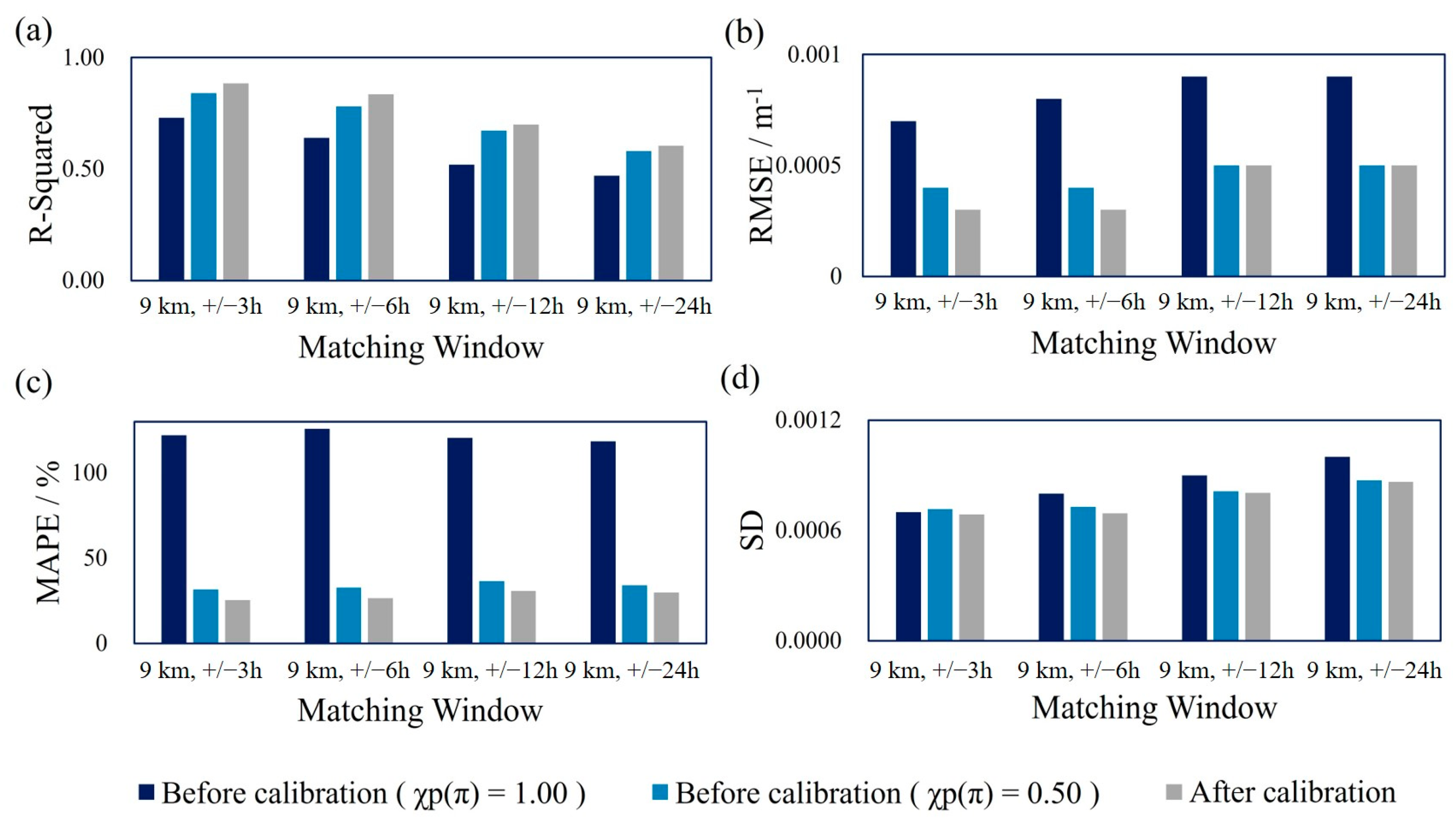
3.3. Comparison before and after Seasonal χp(π) Calibration

We utilized the average χp(π) conversion factor across the 12 distinct spatiotemporal matching windows to rectify the CALIOP bbp product. Subsequently, we evaluated the product’s performance both before and after the correction. Prior research has underscored the significant impact of altering the β(π)/bbp conversion coefficient on the quality of CALIOP data. For instance, Bission et al. demonstrated varying evaluation results by multiplying β(π)/bbp by a factor of 0.32 [19,20]. Consequently, we employed two different algorithms for evaluation before calibration. One algorithm employed a fixed β(π)/bbp value of 0.16 (χp(π) = 1.00), while the other used a β(π)/bbp value of 0.32 (χp(π) = 0.50). To assess the performance of the corrected products, we established four evaluation windows, each characterized by a 9 km spatial radius and temporal intervals of ±3 h, ±6 h, ±12 h, and ±24 h. These evaluations allowed us to compare the product’s performance among the χp(π) = 1.00 algorithm, the χp(π) = 0.50 algorithm, and after correction by average seasonal χp(π) under different conditions.
The evaluation results show that, in all matching windows, using the χp(π) seasonal average calibration values improved the performance of the products, compared to the algorithms with fixed β(π)/bbp of 0.16 and 0.32 (Figure 8). This indicates that using the χp(π) seasonal average calibration values for correction is effective. Taking the 9 km, ±3 h spatiotemporal matching window as an example, the corrected product exhibited higher R2 (R2after calibration = 0.89, R2χp(π)=1.00 = 0.73, R2χp(π)=0.50 = 0.84), smaller root mean square error (RMSE) (RMSEafter calibration = 3.0 × 10⁻⁴ m−1, RMSEχp(π)=1.00 = 7.0 × 10⁻⁴ m−1, RMSEχp(π)=0.50 = 4.0 × 10⁻⁴ m−1), and smaller mean absolute percent error (MAPE) (MAPEafter calibration = 25.27%, MAPEχp(π)=1.00 = 121.97%, MAPEχp(π)=0.50 = 31.48%). These performance metrics are summarized in Table 2.

4. Discussion

4.1. Effect of Band Conversion Factor

In this study, a calibration was performed on CALIOP VSF-retrieved bbp(532) in global ocean regions using bbp(700) measured by BGC-Argo and bbp(443) measured by MODIS. The seasonal variations in χp(π) were re-examined. During the matching calibration process, because CALIOP estimates bbp values at a wavelength of 532 nm, it was necessary to convert the bbp(700) values from BGC-Argo to bbp(532) and the bbp(443) values from MODIS to bbp(532). To do this, the spectral slope of the bbp values, known as the particle size index (γ, [11]), was obtained through a nonlinear power–law fit to the particle beam attenuation spectrum (with γ as the negative exponent of the power–law). For particles smaller than approximately 20 µm, this parameter is negatively correlated with the mean particle size; smaller values of this parameter correspond to larger mean particle sizes [41].
Lacour et al. used a fixed value of 0.78 for the spectral slope when performing band conversion of BGC-Argo’s bbp product to match CALISPO bbp [19]. In contrast, Bisson et al. derived a variable value from the MODIS-Aqua data [20], and the calculation method for the variable slope is as follows:
γ = 2.2 ( 1 1.2 e 0.9 ( R r s ( 443 ) R r s ( 555 ) ) )
where Rrs represents remote sensing reflectance. Vadakke-Chanat and Jamet compared the differences between estimates of bbp(532) using a fixed slope and a variable slope and found that most values closely aligned with a 1:1 line [22]. However, they also identified a bias resulting in a 40% relative error. Therefore, the choice of spectral slope can also impact the calibration of bbp from other bands to CALIOP bbp, thereby influencing the calculation of χp(π) seasonal variations.

4.2. Effect of Atmospheric Turbulence

When a laser propagates through turbulent atmosphere, fluctuations in the atmospheric refractive index field cause distortions in the laser wavefront, which degrade the laser’s coherence. This degradation weakens the quality of the laser, manifesting in random phase fluctuations, random beam drift, energy redistribution across the beam cross-section (distortion, broadening, fragmentation, etc.), and resulting intensity fluctuations [53,54]. Therefore, the impact of atmospheric turbulence on the conversion factor is also an important aspect.
According to the study by Liao et al. (2023), when vortex electromagnetic waves propagate through a turbulent atmosphere, their amplitude and phase are disturbed, leading to a scintillation effect [55]. Their results indicate that vortex wave data can be used for the inversion of turbulent refractive structure parameters and provide new research directions for atmospheric remote sensing. Therefore, incorporating the refractive structure of atmospheric turbulence in future research could enable a more accurate interpretation of the variability of the conversion factor, thereby improving the inversion accuracy of CALIOP. Additionally, the study by He et al. (2024) reveals stratospheric disturbance information through new detection technology, which is crucial for understanding atmospheric turbulence and quantifying its impact on the conversion factor [56].
We plan to further explore the specific impact of atmospheric turbulence on the conversion factor in future research, and to conduct a comprehensive analysis combining the turbulent refractive structure and stratospheric disturbance information, with the aim of enhancing the accuracy and reliability of inversion methods.

4.3. Regional Differences in χp(π) Based on MODIS

Due to the limited data availability of BGC-Argo floats in certain marine areas, in order to facilitate the study of the regional variations in seasonal differences of χp(π), we employed passive ocean-color-remote-sensing product MODIS bbp to investigate the seasonal changes of χp(π) in 26 global marine regions.
The results of the study revealed three distinct types of patterns in the Global Ocean. The first type, referred to as the “summer peak” type, was identified in 15 regions including 1, 5, 7, 8, 10, 11, 12, 13, 14, 17, 18, 19, 21, 22, and 25 (Figure 9). This type exhibited a distinct seasonal variation with the highest χp(π) values occurring during the summer and gradually decreasing during the autumn and winter seasons. Upon further subdivision, it was observed that in nine of these regions (1, 8, 10, 11, 13, 17, 18, 21, and 25), the χp(π) values during spring were higher than those in autumn and winter. Additionally, in six regions (5, 7, 12, 14, 19, and 22), the χp(π) values during spring were intermediate between those of autumn and winter, while no region displayed lower spring values compared to winter values.
The seasonal variation in χp(π) is predominant in “summer peak” type regions globally, and the primary reason for this seasonal difference lies in the seasonal variations in the shape of phytoplankton particles, as described in Section 2.1. Additionally, the thickness (Dc) and relative refractive index (nc) of phytoplankton shells (membranes) can vary depending on the growth stage. For instance, cell membrane thickness can range from 0.05 to 0.13 µm, and the relative refractive index can vary from 1.06 to 1.22 [57,58]. Hu et al.’s research found that when the shell is very thin (≤0.05 µm), or the refractive index of the shell is low (≤1.06), or both conditions are met, the χp(π) derived from the coated sphere model approximates that of a homogeneous sphere (dashed line). As Dc or nc increases, χp(π) decreases [23]. Therefore, the different growth stages of phytoplankton can lead to variations in χp(π) in different marine regions where they exist.
The second type, labeled as the “decline” type, was identified in seven regions including 3, 4, 8, 15, 16, 20, and 26 (Figure 9). This type exhibited a consistent decrease in χp(π) values from spring to winter. Among these regions, four (4, 8, 15, and 16) displayed a strict decline in values across the seasons. Region 26 also exhibited this strict decline, but data for winter values were unavailable. Region 3 displayed a non-strict decline, with summer values being lower than those in spring and autumn, while maintaining an overall “decline” type trend. Similarly, region 20 lacked winter data, but its general trend aligned with the “decline” type.
The seasonal variation in χp(π) in “decline” type regions is primarily concentrated near the equator and the arctic regions. Compared to “summer peak” type regions, the main difference in “decline” type regions is the absence of a peak advantage during the summer season. There is a strong link between the morphology of phytoplankton cells and their physiological and metabolic processes [59,60,61]. To maximize chloroplast exposure to light, adaptive strategies are employed [62]. It appears that the optimal morphological adaptation strategy for phytoplankton is to maintain an optimal surface-to-volume ratio (S/V), which facilitates rapid surface exchange, more efficient use of light and nutrients, and reduces sinking losses [63]. Changes in the surface-to-volume ratio result in corresponding changes in χp(π). Because the physicochemical environmental conditions in equatorial and arctic regions during the summer season differ from those in other regions, phytoplankton adopt different morphological adaptation strategies, resulting in distinct seasonal variations in χp(π).
The third type, denoted as the “autumn pole” type, emerged in three regions: 6, 23, and 24 (Figure 9). This type was characterized by the autumn χp(π) values being either the highest or lowest among the four seasons. Sub-categorically, regions 23 and 24 exhibited the autumn peak pattern, with the highest values observed during that season. In contrast, region 6 displayed the autumn trough pattern, with the lowest values occurring during autumn.
In summary, the study identified three distinct seasonal patterns—summer peak, decline, and autumn pole—in the examined regions based on variations in χp(π) values throughout the four seasons. These findings provide valuable insights into the complex seasonal dynamics and variations in the studied regions.

5. Conclusions

Due to the difficulty in obtaining in situ data for the 180° particle volume-scattering function, there is a lack of investigation and understanding of the natural variations in the key conversion coefficient χp(π) on a global, large-scale, and long-term basis. The persistent deployment of BGC-Argo floats and the prolonged accumulation of data through its wide array have furnished a substantial repository of in situ data. This has enabled the in-depth scrutiny of the critical conversion factor, χp(π), which is fundamental to CALIOP’s inversion of bbp. Using the in situ bbp readings from the BGC-Argo floats, we were able to determine calibrated χp(π) values. These values serve as a central conversion coefficient in CALIOP’s bbp inversion procedure across diverse seasons. This study revealed noticeable seasonal deviations in χp(π). In addition, the existing bbp inversion model is still relatively coarse, with many assumptions carrying certain uncertainties. The error caused by using a constant conversion factor in the current inversion algorithm cannot be ignored. Therefore, by focusing on the conversion factor, the CALIOP bbp inversion model is corrected to further improve the accuracy of the CALIOP bbp product.
(1)
Consistent seasonal fluctuations in the χp(π) values were seen at varying spatiotemporal scales, with the highest values recorded in summer (0.46–0.48) and lowest in winter (0.33–0.36), while fall and spring values remained in the middle range. The average calibrated conversion factor χp(π) through the 12 matching windows was computed; 0.40 for spring, 0.48 for summer, 0.43 for fall, and 0.35 for winter.
(2)
An analysis of the diurnal differences in χp(π) showed daytime values to be slightly higher than nighttime values in all seasons, with the highest daytime and lowest nighttime values in summer and winter, respectively, matching the overall daily trend in χp(π).
(3)
The passive ocean-color-remote-sensing product, MODIS bbp, was used to observe the seasonal fluctuations in χp(π) in 26 global sea areas, revealing three major seasonal variation patterns: “summer peak”, “decline”, and “autumn pole”. The “summer peak” was the most prevalent, aligning with the trend detected through the BGC-Argo floats.
(4)
After factoring in the seasonal variations in χp(π), the CALIOP bbp product was duly calibrated, yielding improved statistical results. The coefficient of determination increased noticeably from 0.84 to 0.89 post-calibration. Additionally, the root mean square error dropped from 4.0 × 10⁻⁴ m−1 to 3.0 × 10⁻⁴ m−1, and the mean absolute percentage error saw a considerable reduction from 31.48% to 25.27%.
The matching points between BGC-Argo floats and CALIOP obtained in this study from 2010 to 2017 are limited in number. However, we believe that with the widespread deployment of BGC-Argo floats and the increase in accumulation time, more comprehensive matching points and finer matching scales will be generated. This will allow for the acquisition of key conversion factors χp(π) across different ocean regions globally, thereby further improving the inversion accuracy of CALIPSO bbp products.

Author Contributions

Conceptualization, M.S. and P.C.; methodology, M.S.; software, M.S.; validation, M.S., P.C., Y.L. and Z.Z.; formal analysis, M.S.; resources, Z.Z.; data curation, M.S.; writing—original draft preparation, M.S.; writing—review and editing, M.S.; visualization, M.S.; supervision, P.C.; project administration, P.C.; funding acquisition, P.C. All authors have read and agreed to the published version of the manuscript.

Funding

This research was funded by the National Natural Science Foundation (42322606; 42276180; 61991453); the National Key Research and Development Program of China (2022YFB3902603; 2022YFC3104200); Key R&D Program of Shandong Province, China (2023ZLYS01); the Key Special Project for Introduced Talents Team of Southern Marine Science and Engineering Guangdong Laboratory (GML2021GD0809); the Donghai Laboratory Preresearch Project (DH2022ZY0003); and the Key Research and Development Program of Zhejiang Province (grant No. 2020C03100).

Data Availability Statement

The data presented in this study were derived from the following resources: CALIOP data from NASA Langley Research Center through the Atmospheric Sciences Data Center (https://asdc.larc.nasa.gov/data/CALIPSO/ (accessed on 9 June 2022)), MODIS products from the NASA Marine Biology Processing Group and Glob Color (https://oceandata.sci.gsfc.nasa.gov/ (accessed on 9 June 2022)), and BGC-Argo data from the International Argo Program and the CORIOLIS project (https://biogeochemical-argo.org/data-access.php (accessed on 9 June 2022)).

Acknowledgments

We would like to acknowledge the valuable contributions of the reviewers whose suggestions significantly enhanced the presentation of this paper.

Conflicts of Interest

The authors declare no conflicts of interest.

References

  1. Tyler, J.; Richardson, W. Nephelometer for the Measurement of Volume Scattering Function in Situ. J. Opt. Soc. Am. 1958, 48, 354–357. [Google Scholar] [CrossRef]
  2. Sullivan, J.M.; Twardowski, M.S. Angular shape of the oceanic particulate volume scattering function in the backward direction. Appl. Opt. 2009, 48, 6811–6819. [Google Scholar] [CrossRef] [PubMed]
  3. Lee, M.; Korchemkina, E. Volume Scattering Function of Seawater; Springer: Berlin/Heidelberg, Germany, 2018; pp. 151–195. [Google Scholar]
  4. Chami, M.; Shybanov, E.B.; Khomenko, G.A.; Lee, M.E.G.; Martynov, O.V.; Korotaev, G.K. Spectral variation of the volume scattering function measured over the full range of scattering angles in a coastal environment. Appl. Opt. 2006, 45, 3605–3619. [Google Scholar] [CrossRef] [PubMed]
  5. Berthon, J.-F.; Shybanov, E.; Lee, M.E.G.; Zibordi, G. Measurements and modeling of the volume scattering function in the coastal northern Adriatic Sea. Appl. Opt. 2007, 46, 5189–5203. [Google Scholar] [CrossRef] [PubMed]
  6. Moore, C.; Barnard, A.; Fietzek, P.; Lewis, M.R.; Sosik, H.M.; White, S.; Zielinski, O. Optical tools for ocean monitoring and research. Ocean Sci. 2009, 5, 661–684. [Google Scholar] [CrossRef]
  7. Sokolov, A.; Chami, M.; Dmitriev, E.; Khomenko, G. Parameterization of volume scattering function of coastal waters based on the statistical approach. Opt. Express 2010, 18, 4615–4636. [Google Scholar] [CrossRef]
  8. Churnside, J.; McCarty, B.; Lu, X. Subsurface Ocean Signals from an Orbiting Polarization Lidar. Remote Sens. 2013, 5, 3457–3475. [Google Scholar] [CrossRef]
  9. Sauzède, R.; Claustre, H.; Uitz, J.; Jamet, C.; Dall’Olmo, G.; D’Ortenzio, F.; Gentili, B.; Poteau, A.; Schmechtig, C. A neural network-based method for merging ocean color and Argo data to extend surface bio-optical properties to depth: Retrieval of the particulate backscattering coefficient. J. Geophys. Res. Ocean. 2016, 121, 2552–2571. [Google Scholar] [CrossRef]
  10. Behrenfeld, M.J.; Hu, Y.; O’Malley, R.T.; Boss, E.S.; Hostetler, C.A.; Siegel, D.A.; Sarmiento, J.L.; Schulien, J.; Hair, J.W.; Lu, X.; et al. Annual boom–bust cycles of polar phytoplankton biomass revealed by space-based lidar. Nat. Geosci. 2017, 10, 118–122. [Google Scholar] [CrossRef]
  11. Boss, E.; Pegau, W. Relationship of Light Scattering at an Angle in the Backward Direction to the Backscattering Coefficient. Appl. Opt. 2001, 40, 5503–5507. [Google Scholar] [CrossRef]
  12. Churnside, J.; Tatarskii, V.; Wilson, J. Oceanographic Lidar Attenuation Coefficients and Signal Fluctuations Measured from a Ship in the Southern California Bight. Appl. Opt. 1998, 37, 3105–3112. [Google Scholar] [CrossRef] [PubMed]
  13. Xue, Y.; Wen, Y.-M.; Duan, Z.-M.; Zhang, W.; Liu, F.-L. Retrieval of Chlorophyll a Concentration in Water Considering High-Concentration Samples and Spectral Absorption Characteristics. Sustainability 2021, 13, 12144. [Google Scholar] [CrossRef]
  14. Lu, X.; Hu, Y.; Pelon, J.; Trepte, C.; Liu, K.; Rodier, S.; Zeng, S.; Lucker, P.; Verhappen, R.; Wilson, J.; et al. Retrieval of ocean subsurface particulate backscattering coefficient from space-borne CALIOP lidar measurements. Opt. Express 2016, 24, 29001–29008. [Google Scholar] [CrossRef] [PubMed]
  15. Winker, D.; Vaughan, M.; Omar, A.; Hu, Y.; Powell, K.; Liu, Z.; Hunt, W.; Young, S. Overview of the CALIPSO mission and CALIOP data processing algorithms. J. Atmos. Ocean. Technol. 2009, 26, 2310–2323. [Google Scholar] [CrossRef]
  16. Behrenfeld, M.; Hu, Y.; Bisson, K.; Lu, X.; Westberry, T. Retrieval of ocean optical and plankton properties with the satellite Cloud-Aerosol Lidar with Orthogonal Polarization (CALIOP) sensor: Background, data processing, and validation status. Remote Sens. Environ. 2022, 281, 113235. [Google Scholar] [CrossRef]
  17. Liu, D.; Xu, P.; Zhou, Y.; Chen, W.; Han, B.; Zhu, X.; He, Y.; Mao, Z.; Le, C.; Chen, P.; et al. Lidar Remote Sensing of Seawater Optical Properties: Experiment and Monte Carlo Simulation. IEEE Trans. Geosci. Remote Sens. 2019, 57, 9489–9498. [Google Scholar] [CrossRef]
  18. Chen, P.; Jamet, C.; Liu, D. LiDAR Remote Sensing for Vertical Distribution of Seawater Optical Properties and Chlorophyll-a from the East China Sea to the South China Sea. IEEE Trans. Geosci. Remote Sens. 2022, 60, 1–21. [Google Scholar] [CrossRef]
  19. Lacour, L.; Larouche, R.; Babin, M. In situ evaluation of spaceborne CALIOP lidar measurements of the upper-ocean particle backscattering coefficient. Opt. Express 2020, 28, 26989–26999. [Google Scholar] [CrossRef] [PubMed]
  20. Bisson, K.; Boss, E.; Werdell, P.; Ibrahim, A.; Behrenfeld, M. Particulate Backscattering in the Global Ocean: A Comparison of Independent Assessments. Geophys. Res. Lett. 2021, 48, e2020GL090909. [Google Scholar] [CrossRef]
  21. Sun, M.; Chen, P.; Zhang, Z.; Zhong, C.; Xie, C.; Pan, D. Evaluation of the CALIPSO Lidar-observed particulate backscattering coefficient on different spatiotemporal matchup scales. Front. Mar. Sci. 2023, 10, 1181268. [Google Scholar] [CrossRef]
  22. Vadakke Chanat, S.; Jamet, C. Validation protocol for the evaluation of space-borne lidar particulate back-scattering coefficient bbp. Front. Remote Sens. 2023, 4, 1194580. [Google Scholar] [CrossRef]
  23. Hu, L.; Zhang, X.; Xiong, Y.; Gray, D.J.; He, M.-X. Variability of relationship between the volume scattering function at 180° and the backscattering coefficient for aquatic particles. Appl. Opt. 2020, 59, C31–C41. [Google Scholar] [CrossRef]
  24. Hair, J.; Hostetler, C.; Hu, Y.; Behrenfeld, M.; Butler, C.; Harper, D.; Hare, R.; Berkoff, T.; Cook, A.; Collins, J.; et al. Combined Atmospheric and Ocean Profiling from an Airborne High Spectral Resolution Lidar. EPJ Web Conf. 2016, 119, 22001. [Google Scholar] [CrossRef]
  25. Zhang, X.; Boss, E.; Gray, D. Significance of scattering by oceanic particles at angles around 120 degree. Opt. Express 2014, 22, 31329–31336. [Google Scholar] [CrossRef]
  26. Lee, J.H.; Churnside, J.H.; Marchbanks, R.D.; Donaghay, P.L.; Sullivan, J.M. Oceanographic lidar profiles compared with estimates from in situ optical measurements. Appl. Opt. 2013, 52, 786–794. [Google Scholar] [CrossRef]
  27. Churnside, J.; Sullivan, J.; Twardowski, M. Lidar extinction-to-backscatter ratio of the ocean. Opt. Express 2014, 22, 18698–18706. [Google Scholar] [CrossRef]
  28. Churnside, J.H.; Marchbanks, R.D. Subsurface plankton layers in the Arctic Ocean. Geophys. Res. Lett. 2015, 42, 4896–4902. [Google Scholar] [CrossRef]
  29. Zhang, X.; Hu, L.; Gray, D.; Xiong, Y. The shape of particle backscattering in theNorth Pacific Ocean: The χ factor. Appl. Opt. 2021, 60, 1260–1266. [Google Scholar] [CrossRef]
  30. Maffione, R.A.; Honey, R.C. Instrument for measuring the volume scattering function in the backward direction. In Ocean Optics XI; SPIE: St. Bellingham, WA, USA, 1992; pp. 15–26. [Google Scholar]
  31. Chami, M.; Thirouard, A.; Harmel, T. POLVSM (Polarized Volume Scattering Meter) instrument: An innovative device to measure the directional and polarized scattering properties of hydrosols. Opt. Express 2014, 22, 26403–26428. [Google Scholar] [CrossRef]
  32. Hu, L.; Zhang, X.; Perry, M.J. Light scattering by pure seawater: Effect of pressure. Deep Sea Res. Part I Oceanogr. Res. Pap. 2019, 146, 103–109. [Google Scholar] [CrossRef]
  33. Algorri, J.F.; Roldán-Varona, P.; Fernández-Manteca, M.G.; López-Higuera, J.M.; Rodriguez-Cobo, L.; Cobo-García, A. Photonic Microfluidic Technologies for Phytoplankton Research. Biosensors 2022, 12, 1024. [Google Scholar] [CrossRef]
  34. Poteau, A.; Boss, E.; Claustre, H. Particulate concentration and seasonal dynamics in the mesopelagic ocean based on the backscattering coefficient measured with Biogeochemical-Argo floats. Geophys. Res. Lett. 2017, 44, 6933–6939. [Google Scholar] [CrossRef]
  35. Barbieux, M.; Uitz, J.; Bricaud, A.; Organelli, E.; Poteau, A.; Schmechtig, C.; Gentili, B.; Obolensky, G.; Leymarie, E.; Penkerc’h, C.; et al. Assessing the Variability in the Relationship Between the Particulate Backscattering Coefficient and the Chlorophyll a Concentration from a Global Biogeochemical-Argo Database. J. Geophys. Res. Ocean. 2018, 123, 1229–1250. [Google Scholar] [CrossRef]
  36. Zhang, X.; Hu, L. Estimating scattering of pure water from density fluctuation of the refractive index. Opt. Express 2009, 17, 1671–1678. [Google Scholar] [CrossRef]
  37. Sullivan, J.; Twardowski, M.; Zaneveld, J.R.V.; Moore, C. Measuring optical backscattering in water. Light Scatt. Rev. 2013, 7, 189–224. [Google Scholar]
  38. Organelli, E.; Claustre, H.; Bricaud, A.; Schmechtig, C.; Poteau, A.; Xing, X.; Prieur, L.; D’Ortenzio, F.; Dall’Olmo, G.; Vellucci, V. A Novel Near-Real-Time Quality-Control Procedure for Radiometric Profiles Measured by Bio-Argo Floats: Protocols and Performances. J. Atmos. Ocean. Technol. 2016, 33, 160303130530002. [Google Scholar] [CrossRef]
  39. Dall’Olmo, G.; Bhaskar TVS, U.; Bittig, H.; Boss, E.; Brewster, J.; Claustre, H.; Donnelly, M.; Maurer, T.; Nicholson, D.; Paba, V.; et al. Real-time quality control of optical backscattering data from Biogeochemical-Argo floats. Open Res. Eur. 2022, 2, 118. [Google Scholar] [CrossRef]
  40. Briggs, N.; Perry, M.J.; Cetinić, I.; Lee, C.; D’Asaro, E.; Gray, A.; Rehm, E. High-resolution observations of aggregate flux during a sub-polar North Atlantic spring bloom. Deep Sea Res. Part I Oceanogr. Res. Pap. 2011, 58, 1031–1039. [Google Scholar] [CrossRef]
  41. Boss, E.; Picheral, M.; Leeuw, T.; Chase, A.; Karsenti, E.; Gorsky, G.; Taylor, L.; Slade, W.; Ras, J.; Claustre, H. The characteristics of particulate absorption, scattering and attenuation coefficients in the surface ocean; Contribution of the Tara Oceans expedition. Methods Oceanogr. 2013, 7, 52–62. [Google Scholar] [CrossRef]
  42. Behrenfeld, M.; Gaube, P.; Penna, A.; O’Malley, R.; Burt, W.; Hu, Y.; Bontempi, P.; Steinberg, D.; Boss, E.; Siegel, D.; et al. Global satellite-observed daily vertical migrations of ocean animals. Nature 2019, 576. [Google Scholar] [CrossRef]
  43. Kokhanovsky, A.A. Parameterization of the Mueller matrix of oceanic waters. J. Geophys. Res. 2003, 108, 257–261. [Google Scholar] [CrossRef]
  44. Voss, K.J.; Fry, E.S. Measurement of the Mueller matrix for ocean water. Appl. Opt. 1984, 23, 4427–4439. [Google Scholar] [CrossRef]
  45. Hu, Y.; Stamnes, K.; Vaughan, M.; Pelon, J.; Weimer, C.; Wu, D.; Cisewski, M.; Sun, W.; Yang, P.; Lin, B.; et al. Sea surface wind speed estimation from space-based lidar measurements. Atmos. Chem. Phys. 2008, 8, 3593–3601. [Google Scholar] [CrossRef]
  46. Churnside, J.H. Polarization effects on oceanographic lidar. Opt. Express 2008, 16, 1196–1207. [Google Scholar] [CrossRef]
  47. Haëntjens, N.; Boss, E.; Talley, L.D. Revisiting Ocean Color algorithms for chlorophyll a and particulate organic carbon in the Southern Ocean using biogeochemical floats. J. Geophys. Res. Ocean. 2017, 122, 6583–6593. [Google Scholar] [CrossRef]
  48. Zhang, X.; Hu, L.; He, M.-X. Scattering by pure seawater: Effect of salinity. Opt. Express 2009, 17, 5698–5710. [Google Scholar] [CrossRef]
  49. Stramski, D.; Bricaud, A.; Morel, A. Modeling the inherent optical properties of the ocean based on the detailed composition of the planktonic community. Appl. Opt. 2001, 40, 2929–2945. [Google Scholar] [CrossRef]
  50. Zhang, X.; Twardowski, M.; Lewis, M. Retrieving composition and sizes of oceanic particle subpopulations from the volume scattering function. Appl. Opt. 2011, 50, 1240–1259. [Google Scholar] [CrossRef]
  51. Pulina, S.; Stanca, E.; Luglié, A.; Satta, C.T.; Padedda, B.M. Phytoplankton cell geometric shapes along Mediterranean seasonal environmental variability in natural and artificial lakes. J. Plankton Res. 2022, 44, 208–223. [Google Scholar] [CrossRef]
  52. Ahmed, A.; Madhusoodhanan, R.; Yamamoto, T.; Fernandes, L.; Al-Said, T.; Nithyanandan, M.; Thuslim, F.; Al-Zakri, W.; Al-Yamani, F. Analysis of phytoplankton variations and community structure in Kuwait Bay, Northwestern Arabian Gulf. J. Sea Res. 2022, 180, 102163. [Google Scholar] [CrossRef]
  53. Yang, X.; Gao, M. Fluctuation characteristics of laser transmissions in atmospheric turbulence. Optik 2020, 202, 163624. [Google Scholar] [CrossRef]
  54. Davis, J.I. Consideration of atmospheric turbulence in laser systems design. Appl. Opt. 1966, 5, 139–147. [Google Scholar] [CrossRef]
  55. Liao, Q.; Sheng, Z.; Zhou, S.; Guo, P.; Long, Z.; He, M.; Guan, J. A Preliminary Study on the Inversion Method for the Refraction Structure Parameter from Vortex Electromagnetic Waves. Remote Sens. 2023, 15, 3140. [Google Scholar] [CrossRef]
  56. He, Y.; Zhu, X.; Sheng, Z.; He, M. Identification of stratospheric disturbance information in China based on the round-trip intelligent sounding system. Atmos. Chem. Phys. 2024, 24, 3839–3856. [Google Scholar] [CrossRef]
  57. Meyer, R.A. Light scattering from biological cells: Dependence of backscatter radiation on membrane thickness and refractive index. Appl. Opt. 1979, 18, 585–588. [Google Scholar] [CrossRef]
  58. Bernard, S.; Probyn, T.; Quirantes, A. Simulating the optical properties of phytoplankton cells using a two-layered spherical geometry. Biogeosci. Discuss 2009, 6, 1497–1563. [Google Scholar]
  59. Litchman, E.; Klausmeier, C.; Schofield, O.; Falkowski, P. The role of functional traits and trade-offs in structuring phytoplankton communities: Scaling from cellular to ecosystem level. Ecol. Lett. 2007, 10, 1170–1181. [Google Scholar] [CrossRef]
  60. Litchman, E.; Klausmeier, C.A. Trait-Based Community Ecology of Phytoplankton. Annu. Rev. Ecol. Evol. Syst. 2008, 39, 615–639. [Google Scholar] [CrossRef]
  61. Van de Waal, D.B.; Litchman, E. Multiple global change stressor effects on phytoplankton nutrient acquisition in a future ocean. Philos. Trans. R. Soc. B 2020, 375, 20190706. [Google Scholar] [CrossRef]
  62. Bernardi Aubry, F.; Pugnetti, A.; Roselli, L.; Stanca, E.; Acri, F.; Finotto, S.; Basset, A. Phytoplankton morphological traits in a nutrient-enriched, turbulent Mediterranean microtidal lagoon. J. Plankton Res. 2017, 39, 564–576. [Google Scholar] [CrossRef]
  63. Reynolds, C.S. The Ecology of Phytoplankton; Cambridge University Press: Cambridge, UK, 2006. [Google Scholar]
Figure 1. A comparison of spatial distribution and quantity of BGC-Argo floats after quality control. (a) illustrates the spatial distribution of BGC-Argo buoys; (b) shows the comparison of the number of buoys with different quality control factors.
Remotesensing 16 02704 g001
Figure 2. The results for matching points of BGC-Argo and CALIOP using different spatial windows, including a 9 km window (a), a 50 km window (b), and a 1° × 1° window (c). (d) shows a comparison of the number of matching points across different spatiotemporal windows.
Remotesensing 16 02704 g002
Figure 3. The comparison between CALIOP and BGC-Argo bbp(532 nm) matchups for a 9 km spatial window and a ±3 h time window, as well as the comparison between CALIOP and MODIS bbp (532 nm) matchups for a 9 km spatial window and a ±12 h time window. (a,b) denote the fitting results of CALIOP bbp(532) using the χp(π) = 1.00 algorithm and BGC-Argo bbp(532) estimates matching; (c,d) denote the fitting results of CALIOP bbp(532) using the χp(π) = 0.50 algorithm and BGC-Argo bbp(532) estimates matching; and (e,f) denote the fitting results of CALIOP bbp(532) using the χp(π) = 0.50 algorithm and MODIS bbp(532) estimates matching.
Remotesensing 16 02704 g003
Figure 4. The flow chart of this study.
Remotesensing 16 02704 g004
Figure 5. The comparison of χp(π) values of conversion coefficients for different seasons within different spatial–temporal matching windows. (a) shows the χp(π) calibration results with a 9 km spatial window match; (b) shows the calibration results with a 50 km spatial window match; and (c) shows the calibration results with a 1° × 1° spatial window match.
Remotesensing 16 02704 g005
Figure 6. Line plots of the seasonal variation of χp(π) for 12 spatiotemporally matched windows. (a) A line graph representing the seasonal variation of χp(π) for each spatial–temporal window; (b) A bar graph representing the seasonal variation of the mean χp(π).
Remotesensing 16 02704 g006
Figure 7. Variations of χp(π) values between day and night for different seasons under a 1° × 1° spatial matching window. (a) presents comparisons of χp(π) calibration results between day and night for various seasons with a ±12 h time matching window; (b) shows comparisons of χp(π) calibration results between day and night for various seasons with a ±24 h time matching window; (c) displays bar graphs illustrating comparisons of χp(π) calibration results between day and night for various seasons with a ±12 h time matching window; and (d) presents bar graphs for comparisons of χp(π) calibration results between day and night for various seasons with a ±24 h time matching window.
Remotesensing 16 02704 g007
Figure 8. Performance comparison of CALIOP bbp products before and after calibration in a 9 km spatial window. (a) R2, (b) RMSE, (c) MAPE, and (d) SD Based on BGC-Argo Evaluation.
Remotesensing 16 02704 g008
Figure 9. MODIS-corrected χp(π) seasonal line plots for various sea areas around the globe.
Remotesensing 16 02704 g009
Table 1. Summary of Datasets Including Parameters, Origin, Period, Web Source, and Resolution.
ParametersData OriginPeriodWeb SourceResolution
bbp(700), DepthBGC-Argo2010–2017ftp://ftp.ifremer.fr/ifremer/argo/ (accessed on 9 June 2022)Variable
bbp(532), timeCALIOP2010–2017http://orca.science.oregonstate.edu/lidar_nature_2019.php (accessed on 9 June 2022)16-day visit time
70 m footprint size
bbp(443), Kd(490)MODIS-Aqua2010–2017https://search.earthdata.nasa.gov/ (accessed on 9 June 2022)monthly averaged
9 km
Table 2. Performance comparison of CALIOP bbp before and after calibration in 9 km spatial windows.
Space WindowTime WindowAfter Calibration
NR-SquaredRMSE/m−1MAPE/%SD
9 km±3 h430.893.0 × 10−425.277.0 × 10−4
±6 h500.843.0 × 10−426.367.0 × 10−4
±12 h870.705.0 × 10−430.728.0 × 10−4
±24 h1470.605.0 × 10−429.899.0 × 10−4
Space WindowTime WindowBefore Calibration (χp(π) = 1.00)
NR-SquaredRMSE/m−1MAPE/%SD
9 km±3 h430.737.0 × 10−4121.977.0 × 10−4
±6 h500.648.0 × 10−4125.748.0 × 10−4
±12 h860.529.0 × 10−4120.599.0 × 10−4
±24 h1470.479.0 × 10−4118.501.0 × 10−3
Space WindowTime WindowBefore Calibration (χp(π) = 0.50)
NR-SquaredRMSE/m−1MAPE/%SD
9 km±3 h440.844.0 × 10−431.487.0 × 10−4
±6 h510.784.0 × 10−432.787.0 × 10−4
±12 h880.675.0 × 10−436.418.0 × 10−4
±24 h1490.585.0 × 10−434.139.0 × 10−4
Disclaimer/Publisher’s Note: The statements, opinions and data contained in all publications are solely those of the individual author(s) and contributor(s) and not of MDPI and/or the editor(s). MDPI and/or the editor(s) disclaim responsibility for any injury to people or property resulting from any ideas, methods, instructions or products referred to in the content.

