Article

Remote Sensing for Mapping Natura 2000 Habitats in the Brière Marshes: Setting Up a Long-Term Monitoring Strategy to Understand Changes

1
Littoral Environnement Télédétection Géomatique, UMR CNRS 6554, Université de Nantes, Campus Tertre, 44312 Nantes, France
2
Laboratoire de Planétologie et Géosciences, UMR CNRS 6112, Université de Nantes, 2 Rue de la Houssinière, 44322 Nantes, France
*
Author to whom correspondence should be addressed.
Remote Sens. 2024, 16(15), 2708; https://doi.org/10.3390/rs16152708
Submission received: 20 June 2024 / Revised: 19 July 2024 / Accepted: 19 July 2024 / Published: 24 July 2024
(This article belongs to the Special Issue Remote Sensing for the Study of the Changes in Wetlands)

Abstract

:
On a global scale, wetlands are suffering from a steady decline in surface area and environmental quality. Protecting them is essential and requires a careful spatialisation of their natural habitats. Traditionally, in our study area, species discrimination for floristic mapping has been achieved through on-site field inventories, but this approach is very time-consuming in these difficult-to-access environments. Usually, the resulting maps are also not spatially exhaustive and are not frequently updated. In this paper, we propose to establish a complete map of the study area using remote sensors and set up a long-term and regular observatory of environmental changes to monitor the evolution of a major French wetland. This methodology combines three dataset acquisition technologies, airborne hyperspectral and WorldView-3 multispectral images, supplemented by LiDAR images, which we compared to evaluate the difference in performances. To do so, we applied the Random Forest supervised classification methods using ground reference areas and compared the out-of-bag score (OOB score) as well as the matrix of confusion resulting from each dataset. Thirteen habitats were discriminated at level 4 of the European Nature Information System (EUNIS) typology, at a spatial resolution of around 1.2 m. We first show that a multispectral image with 19 variables produces results which are almost as good as those produced by a hyperspectral image with 58 variables. The experiment with different features also demonstrates that the use of four bands derived from LiDAR datasets can improve the quality of the classification. Invasive alien species Ludwigia grandiflora and Crassula helmsii were also detected without error which is very interesting when applied to these endangered environments. Therefore, since WV-3 images provide very good results and are easier to acquire than airborne hyperspectral data, we propose to use them going forward for the regular observation of the Brière marshes habitat we initiated.

1. Introduction

Wetlands are among the most productive environments on our planet, playing a vital role in the ecosystem. Their functions and values are now widely recognised [1]: wetlands act as carbon sinks [2]; regulate flooding [3]; improve water quality [4]; and play a major role in the landscape by providing unique habitats for a wide variety of plant and animal species [5].
Worldwide, 3.4 million square kilometres of freshwater wetlands disappeared between the years 1700 and 2020, mainly due to conversion to arable land [6]. This loss is now being amplified by the acceleration of global climate change: rising air temperatures, increased evapotranspiration, and lower winter precipitation [7]. Added to this is the degradation of water quality through eutrophication and the threat of saltwater intrusion [5]. These disturbances are already causing, and will continue to cause in the future, numerous changes in the specific composition of these environments. To monitor and understand these changes, it is essential to have accurate, spatially distributed, and up-to-date information on the species habitats identified by the vegetation specific to wetlands.
Traditionally, species discrimination for floristic mapping is carried out using field inventories [8,9]. Although very accurate, these methods are extremely demanding in terms of human and technical resources, very time-consuming, and almost impracticable for large-scale studies requiring frequent data collection [10,11]. Many wetlands are located in remote areas that are logistically difficult to access and where travelling is often hampered. These factors explain why maps are often not updated for a long time after they have been drawn up.
Remote sensing appears to be an appropriate means of mapping wetland habitats. The possibility of repeated acquisitions allows researchers to detect changes over time, and the digital data resulting from these classifications can be integrated into a geographic information system (GIS) [12,13].
Airborne hyperspectral methods are widely used to discriminate and map wetland vegetation at the species level [8,14,15]. However, their high cost and the difficulty of setting up overflights, where necessary, have led researchers to turn to multispectral satellite remote sensing images to map these environments [16,17,18]. They have the advantage of being cheaper in terms of manpower and material resources, and they are easier and quicker to obtain. In addition, Light Detection And Ranging (LiDAR) data are used to help discriminate between species on the basis of their height or the deformation of the return wave produced by their structure [19,20].
In France, major heritage wetlands are protected by various mechanisms such as the Natural Zone of Interest for Ecology, Flora and Fauna (ZNIEFF), Natura 2000 sites, and regional natural parks. However, they are still declining. As a result, the characterisation and monitoring of these environments have been identified as priority elements of European and regional action programs initiated by local stakeholders [21,22].
The mapping data available for the study area (see Section 2.1 below) are not spatially exhaustive and show a simplification of the habitat mosaics. Some of them have been drawn up entirely on the basis of field surveys between 2017 and 2019 and were time-consuming and people-intensive. Others have not been updated since the 1980s, which means that changes cannot be monitored on a regular basis.
Consequently, the objectives of this study are (1) to draw up an accurate map of the study area habitats by comparing the performance between an airborne hyperspectral image coupled with five LiDAR variables and a multispectral scene from the WorldView-3 satellite (due to its high spatial resolution particularly suitable for classifying wetlands) with one LiDAR variable, and (2) to propose a strategy for setting up a long-term monitoring observatory that will enable the mapping to be updated on a regular basis in the future in order to quantify changes.

2. Materials and Methods
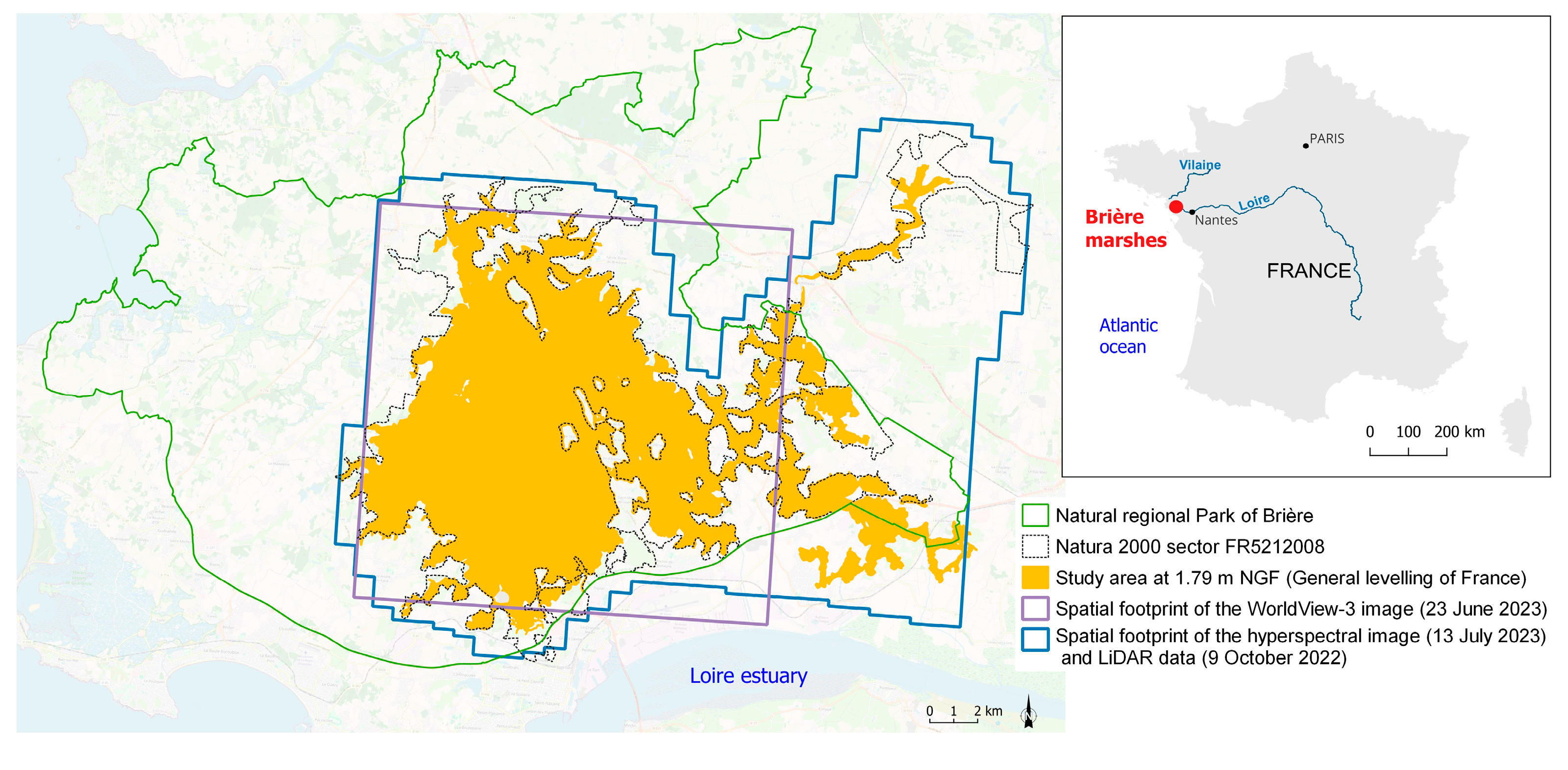
2.1. Study Area

The Natura 2000 site FR5212008 “Grande Brière, Marais de Donges et du Brivet” in Loire-Atlantique is composed of a series of marshy depressions and alluvial marshes located between the Loire estuary to the south and the Vilaine to the north. The site is located within the Brière regional natural park (PnrB) and covers 19,754 ha (Figure 1). For the purposes of the study, a sector at 1.79 m NGF (general levelling of France), corresponding to the maximum flood level, was traced using a digital terrain model from the LiDAR dataset acquired for the study. The territory of the park boasts an exceptional natural heritage. However, it is threatened by a number of pressure points, including the proliferation of invasive exotic species, changes in management methods, the degradation of water bodies, and the effects of climate change [23].

2.2. Data Acquisition

In order to guarantee the implementation of spatial monitoring of the Brière in the future, a hyperspectral airborne image and a WorldView-3 satellite image with very high spatial resolution (1.24 m) (Table 1) were acquired in early summer 2023 (23 June for WorldView-3 image and 13 July for hyperspectral data). This time period was the best compromise for the development of most of the plant communities of the site and made it possible to compensate for the prolonged flooding of some areas of marshland. This choice was complicated by the presence of peripheral plant groups whose phenology was already advanced.
The hyperspectral data were acquired using hyperspectral sensors (Hyspex Mjolnir VS-620 camera from Norsk Elektro Optikk, Skedsmokorset, Norway) from OSUNA (Observatoire des Sciences de l’Univers Nantes Atlantique) on a plane belonging to GEOFIT-expert (a firm of surveyors).
The WorldView-3 image was ordered from European Space Imaging (EUSI). This image is particularly suitable for classifying land and water features because it is the most spatially and spectrally precise satellite constellation. In multispectral mode, the bands provide a clear picture of vegetation properties [24]. As this is a test image, its surface area is smaller than that of the hyperspectral images, and it does not cover the entire study area (Figure 1).
In addition, LiDAR data were acquired on 9 October 2022 by Titan DW600 cameras from Teledyne Optech Incorporated, Vaughan, Ontario, Canada, for the Nantes-Rennes LiDAR platform from OSUNA and OSUR (Observatoire des Sciences de l’Univers de Rennes) on a plane belonging to GEOFIT-expert.
This equipment consists of a topo-bathymetric laser with a wavelength in the green region (channel C3: 532 nm) and a topographic laser with a wavelength in the near infrared (channel C2: 1064 nm) region. For this study, only the topographic informationwas acquired in order to obtain information on the microtopography of the marsh and the structure of the vegetation. This is called fullwaveform (FWF), meaning that the entire return signal is recorded by the sensor.
The complete characteristics of the sensors are shown in Table 1.

2.3. Image Pre-Processing

The airborne hyperspectral image is pre-processed in a combined atmospheric and geometric processing chain with the ATCOR4 [25] and PARGE [26] applications.
The WorldView-3 image is ordered with the “map ready ortho” option and can be used directly without radiometric calibration or orthorectification. Both images are masked using a NIR band threshold value, which can distinguish between pixels on land and water to make classification easier.

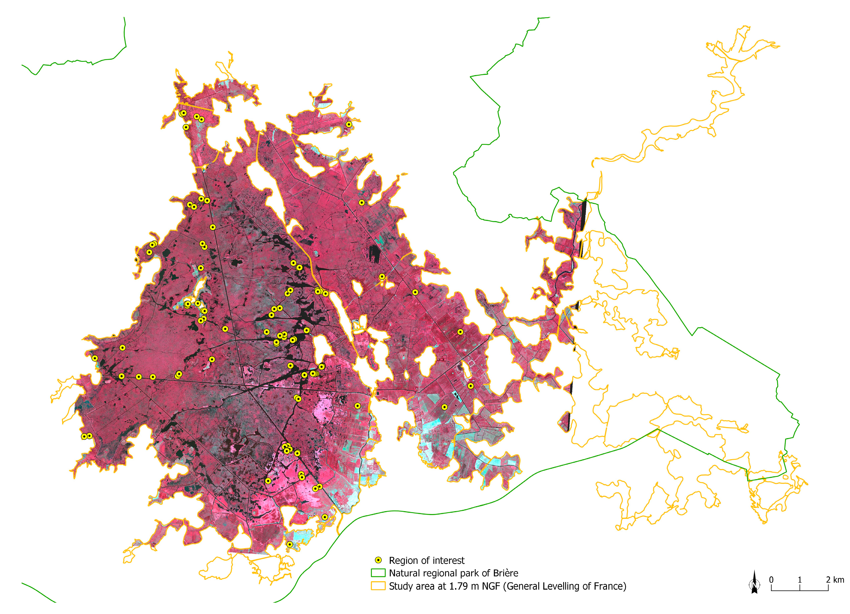
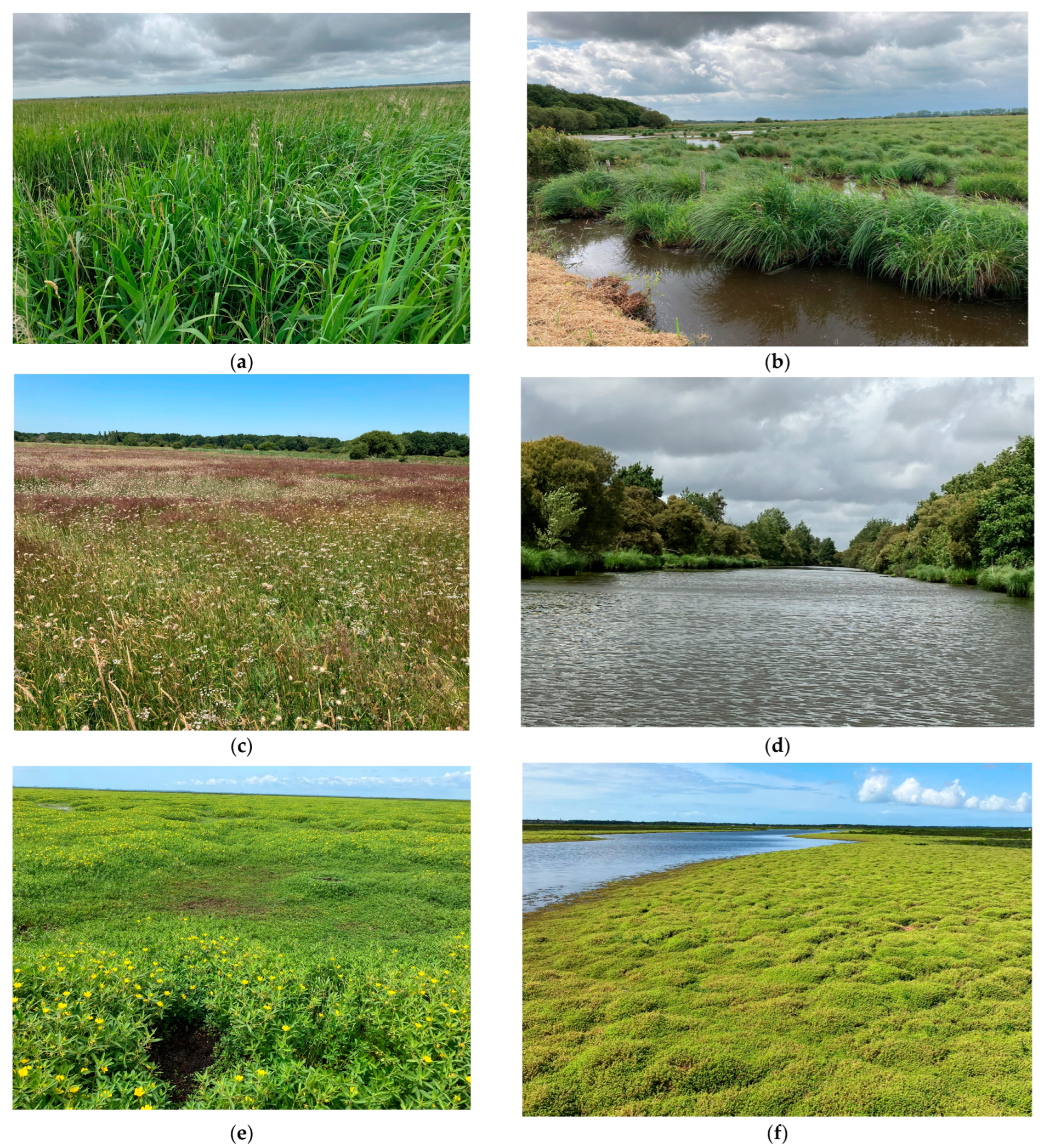
2.4. Field Data Sampling

Field sampling should represent the variability of all communities present in the Natura 2000 area [27,28]. Since we are using the EUNIS typology, the EUNIS guide from the French Biodiversity Agency recommends “paying attention to mosaic habitats, those that are very degraded or in transitional states” [29].
Reasoned choice (non-random) sampling and the definition of a “laboratory” itinerary are generally practised [30]. We selected 74 ground reference areas (Regions of Interest, ROIs) on the basis of the visual interpretation of the WorldView-3 image positioned in areas that are a priori physically and floristically homogeneous, taking into account the full range of textural and spectral variability of the image and preferably along access roads or canals in order to optimise travel times. In the case of fragmented habitats (distributed around the territory in small areas), several replicates of the same colour and texture are selected. Similarly, in the case of very heterogeneous environments, other plots of the same type are selected in order to include all the stages of development and evolution of the same plant formation.
For each type of area to be sampled, we defined the extent of the ROIs to be greater than several times the size of the pixels in the image (at least 3 pixels × 3 pixels). This ensures that the plot is representative of the environment under consideration and not accidental or relict, so that the classification algorithms can learn from it correctly. This procedure has sometimes been difficult to implement because of the spatial distribution of certain small habitats (for example, some lawns do not form continuous grass beds).
These points were then recorded on a smartphone in the MerginMap mobile application [31] by the MerginMap QGis plugin [32] on QGis 3.28 software [33], so that the areas to be surveyed could be easily visualised once in the field.
The surveys corresponding to the points were carried out over the same period as the airborne hyperspectral and WolrdView-3 data acquisition (in 3 sessions on 26 June and 4–5 July) in order to avoid the rapid change in phenology in these environments [8].
Once on the field, the specific composition is determined, as well as the dominant character of each species. When possible, and if the vegetation is no more than 2 metres high, several vertical photos are taken of the survey to confirm the coverage at a later date by another observer if necessary, including one wide-angle shot of the context to keep a record of the reality on the field and better understand the results of the classifications (for example, confusion between similar habitat classes). The centre of the field survey was marked by a white stick placed vertically with a known height (1.10 m), allowing the height to be estimated at a later date if necessary. The GPS coordinates of the survey are taken using a Trimble Geo 7X differential GPS and Trimble TerraSync Professional Software 5.70 [34]. Considering the species it contains, each survey is associated with a level 3 or 4 of the EUNIS (European Nature Information System) typology. EUNIS has a hierarchical typology system, divided into 6 levels, from the most general to the most detailed. It consists of a letter (level 1) to which a number is added as you go down to the finest levels of species, up to 5 numbers (level 6). A table of results is drawn up for each of them (Table 2).
Ten months apart, with no significant changes in plant composition in these buffered environments, we decided to use other botanical surveys conducted in the same period in summer 2022 based on the NGI (National Geographic Institute) BD Ortho IRC (Orthophotographic Database in Infra-Red Colours) of 2020’s textural features. These surveys were primarily carried out to gain a better understanding of the terrain and the dominant species, but they could be added to the pool of ROIs acquired in 2023 if the latter was insufficient for some habitats.
In order to avoid incorporating too much variability in the reference polygons (water holes and small shrubs), their shape was sometimes reworked using a GIS and others were eliminated because they were too close to a contact zone or were too small in area, thus rigorously reducing the number of ROIs to 95, distributed as follows over the study area (Figure 2) and by habitat type (Table 3).
The WV-3 image was acquired two weeks before the HS. In order to save time and ensure that phenology was not too far advanced, the ROIs were defined on the basis of WV-3. Given the poor weather that year, and the fact that the overflight had already been delayed, it was important not to compromise the use of WV-3. Once the hyperspectral flight had been successfully completed, we were able to start the performance comparisons. Since WV-3 did not cover the entire area delimited at 1.79 m and the ROIs had already been characterised, we checked that there were no new shapes and colours (and therefore new habitats) in the sectors of HS not covered by WV-3. If in doubt, they were visited. However, in order to compare the two images on an equal basis, and not to provide additional or different training plots for the HS, we decided to keep only the ground reference data that were common to both images, i.e., that of the smaller scene, WV-3. This explains why there are no ROIs on the right side of the study area.

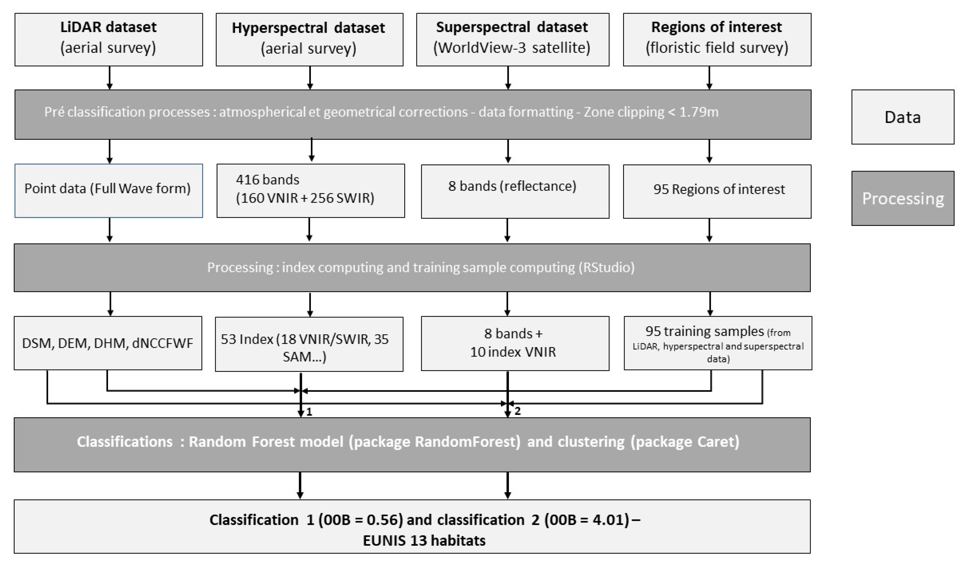
2.5. Classification Method

2.5.1. Variables’ Calculation

Spectral indices commonly used in vegetation mapping were used, adapted to the bands of each type of image. Details of the indices and bibliographical references used are given in Table 4. The hyperspectral image includes bands in the SWIR, enabling the calculation of various indices. This capability allows for comparing the performance of an image with extensive spectral information against a simpler multispectral image.
Spectral Angle Mapping (SAM) calculations are performed on the mean spectral signature of the ground reference areas (ROIs) of each European Nature Information System typology (EUNIS) habitat with the hyperspectral image bands in the VNIR and SWIR being used as additional variables.
Using the LiDAR data, we produced a Digital Surface Model (DSM), a Digital Terrain Model (DTM), and a Digital Height Model (DHM) by the subtraction of both. With the full-waveform signal, we calculated the derived normalised centred cumulative FWF (dNCCFWF) [46] and extracted the intensities at ranges of −1 m, 0.75 m, and +1 m, values that are characteristic of the waveforms of herbaceous vegetation, with the −1 value also making it possible to reject the effects of slopes [19].
Table 5 summarises the variables used in each case.

2.5.2. Classification Algorithm

The classification method used is the “Random Forest” algorithm [47], a supervised classification machine learning algorithm. It was performed with R software (version 3.6.2) (R Development Core Team 2024), using the “randomforest” package [48] and the “caret” package [49]. Various studies have demonstrated its ability to produce accurate vegetation type mappings [50,51,52]. In the RF model, the training data are randomly sampled with replacements, generating “bootstrap” samples. Each “forest” decision tree is built on an “in bag” fraction of the data, which is used to train the algorithm. For each pixel in the remaining fraction (“out of bag”), its class can be predicted by all the decision trees, making it possible to evaluate the final result (OOB score). The OOB score shows the error rate of the trees on the individuals left “out of bag” by the model, the aim being to obtain the lowest possible OOB (for the complete description of the Random Forest model and the OOB score, see Belgiu and Drăguţ, 2016 [53]).
For the tuning of the model, two parameters can be adjusted: “Ntree” that determines the number of decision trees to be generated (Ntree is fixed with the build of a plot with x-axis = number of trees from 0 to 1000) and the y-axis is the error rate; and “Mtry” that sets the number of variables to be randomly selected for each split at each branch of the trees (Mtry =sqrt (p), where p is number of variables).
For our analyses, the relevant parameters were Ntree = 300 and Mtry= 7 for the HS and Mtry = 4 for the WV-3 image (due to difference in variable numbers).
Confusion matrices were produced to complement the OOB score of the Random Forest classifier. A confusion matrix is a table showing the observed data in rows and the data predicted by the algorithm in columns. The diagonal shows the number of individuals with a good classification, i.e., individuals whose prediction matches the observed data. The other values correspond to the individuals misclassified by the algorithm.
The diagram below summarises the overall classification approach (Figure 3).

3. Results

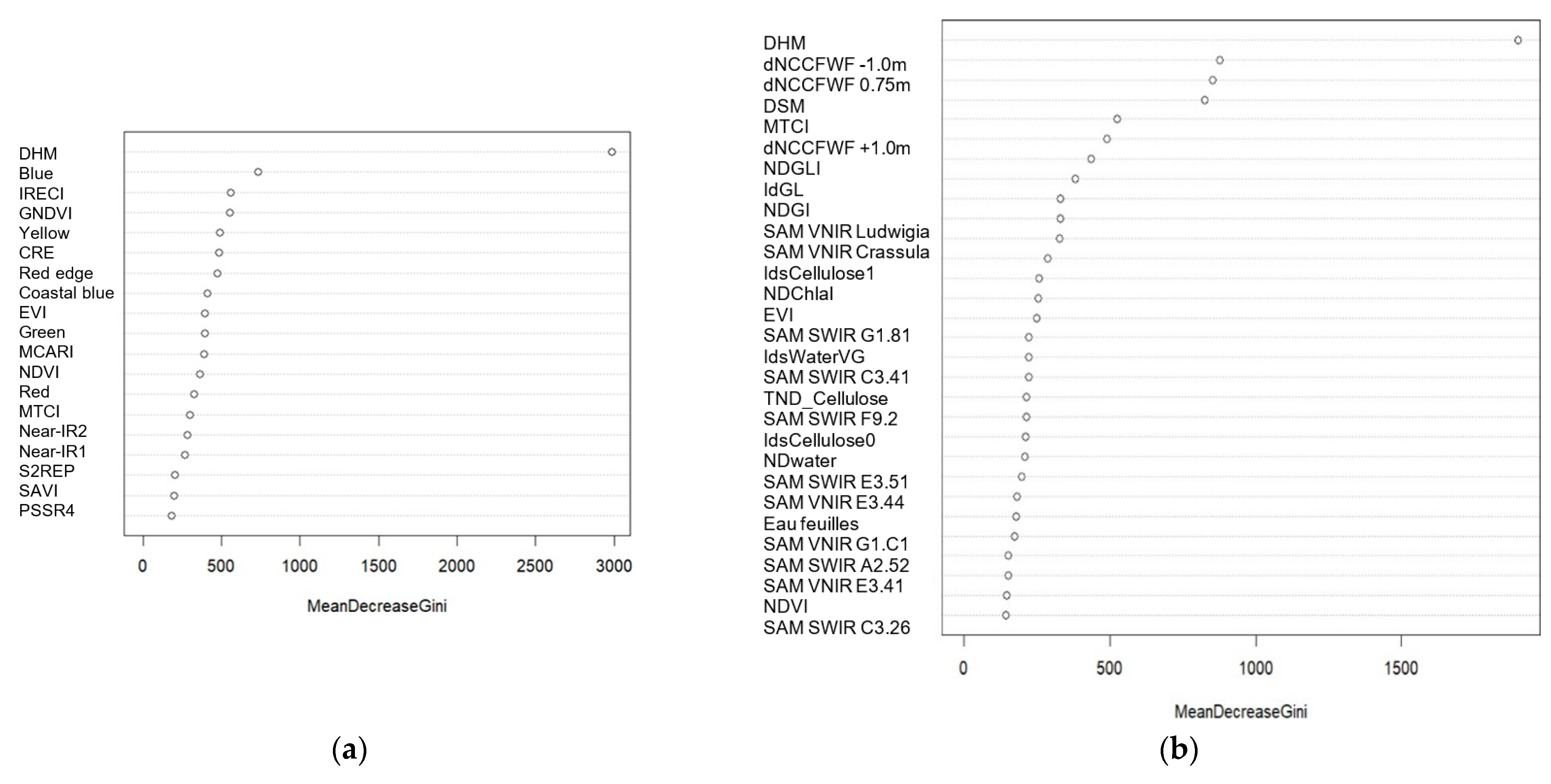
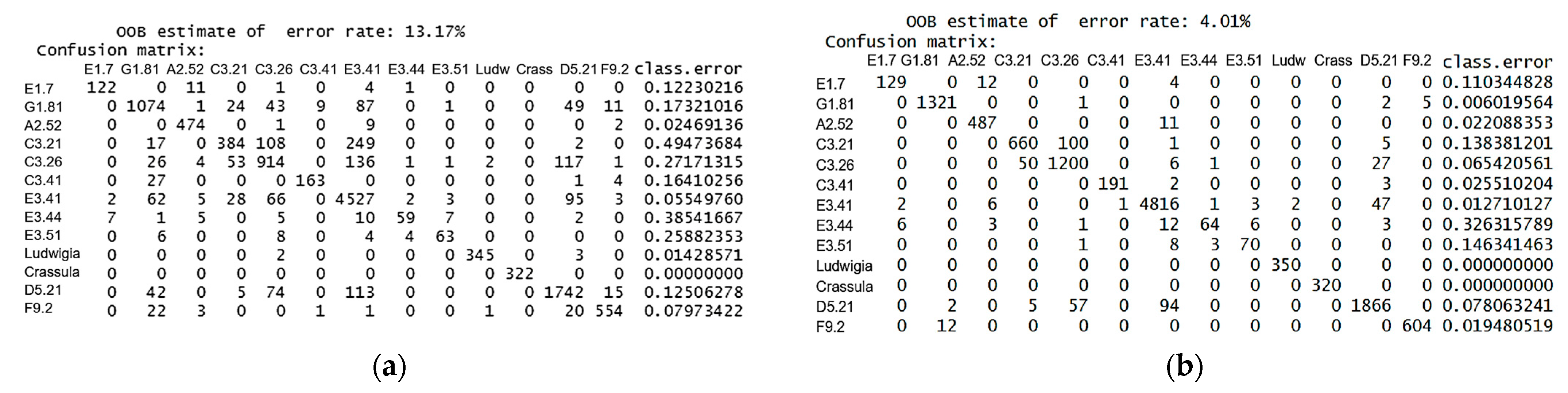
3.1. Variables Importance

The contribution of each variable (spectral bands and vegetation indices) to the accuracy of the RF classification is based on the Mean Decrease Gini (MDG). All the variables are ranked in ascending order according to their importance [48] (Figure 4).
For the WV-3 image, the DHM variable leads the Mean Decrease Gini. The next four most important variables are bands from the image and spectral indices, as follows in order of importance: the blue band, the IRECI, the GNDVI, and the yellow band.
For the hyperspectral image, the DHM is also the most discriminating variable. The four most important variables are all derived from LiDAR: dNCCFWF −1.0 m, dNCCFWF 0.75 m, and the DSM. The first vegetation index (MTCI) only came fifth.
During a first Random Forest classification test on the WV-3 image with only 8 VNIR bands and 10 indices, the OOB was 13.17% (Figure 5). In order to improve the OOB, we decided to add the DHM variable, which was the most discriminating variable for the hyperspectral image. It was not included in the first test because we wanted to make the classification as simple as possible with only the WV-3 variables. This information on the height of the vegetation reduced the OOB to 4.01% (Figure 5). The confusion matrices below show the classes improved by DHM. The table shows the observed data in rows and the data predicted by the algorithm in columns. The diagonal shows the number of individuals with a good classification, i.e., individuals for whom the prediction of the algorithm’s prediction matches the observed data. The other values correspond to the individuals misclassified by the algorithm.
In addition to a substantial improvement in all classes, there was a clear improvement in the Phragmites reedbed class (C3.21), which fell from a class error of 0.49 to 0.14. The flood swards class (C3.44) remains the worst classified, even with the DHM (0.38 compared with 0.32 class error). The invasive exotic species of Ludwigia sp. and Crassula helmsii have no poorly classified pixels. This can be explained by the very dense mat-like appearance of these species, which cannot be confused with any other habitat.

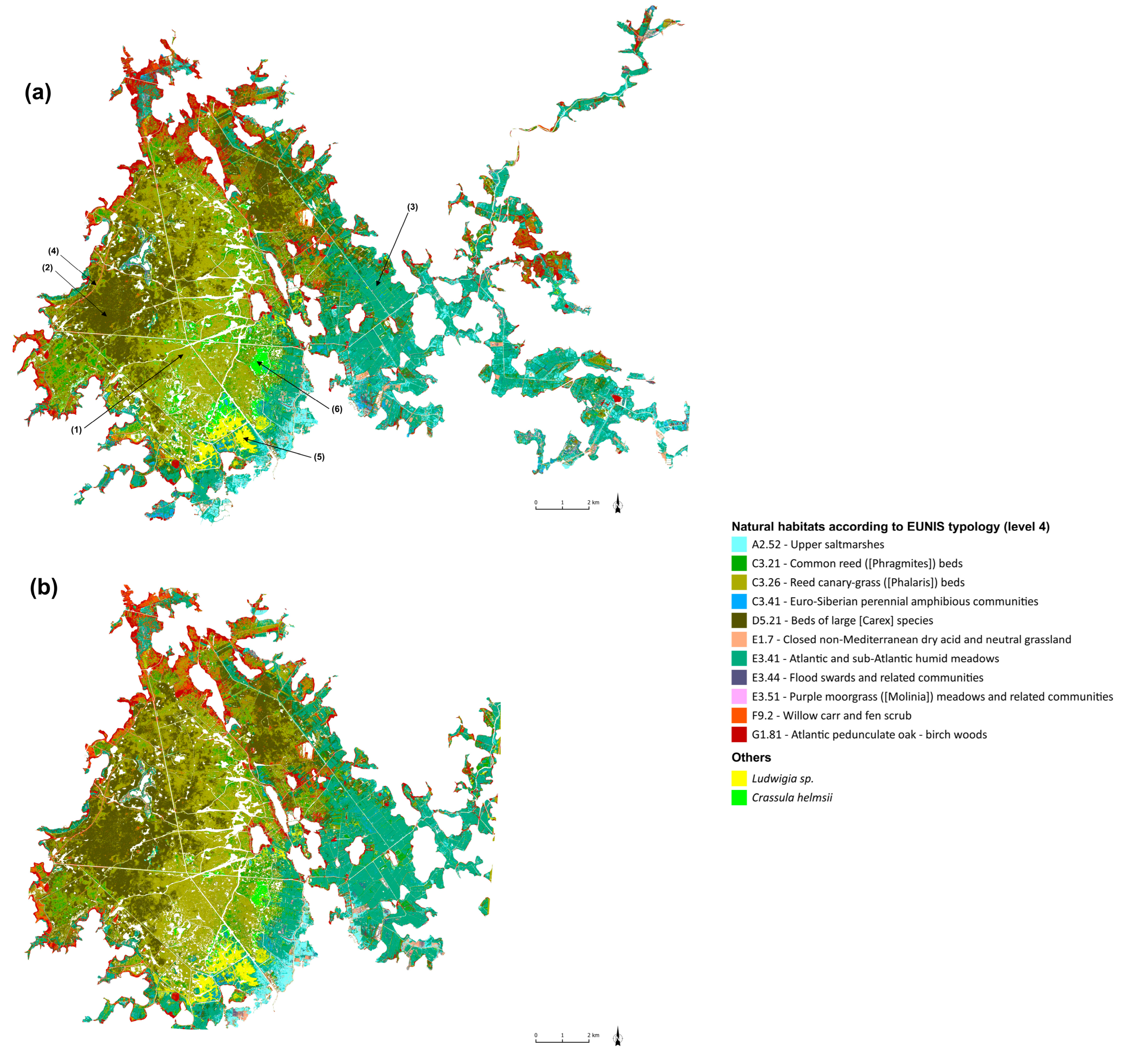
3.2. Up-to-Date Mapping of Habitats

The classification methods applied enabled us to identify 11 species habitats at level 4 of the EUNIS typology (Table 6). In addition to these classic wetland vegetation communities, it is possible to detect two invasive alien plant species of particular concern in the Brière: the Australian swamp stonecrop (Crassula helmsii Kirk) and the Uruguayan primrose willow (Ludwigia grandiflora (Michx.) Greuter & Burdet). The classification results are shown in Figure 6 and pictures of some characteristic habitats are shown on Figure 7.
The EUNIS typology does not include an additional level for habitats E1.7 and F9.2.
They are therefore considered to be at the same level as the other habitats, i.e., level 4.
The overall classification accuracy OOB is 4.01% for the Worldview-3 image and 0.56% for the hyperspectral image.

4. Discussion

4.1. Mapping the Distribution of the Habitats

The initial aim of this study was to establish an up-to-date map of the habitats of the Brière marshes, using remote sensing, in order to monitor and quantify the changes taking place in this complex ecosystem. The mapping method used for this study differs from the traditional approaches used in the area up to now, which consist of scouring the area in selected sectors, as this is very time-consuming and requires a lot of technical and human resources in the field. In this case, there is no need, as 95 targeted points of interest can be used to carry out the classification, eliminating the need for time-consuming surveys and making it possible to get into areas that are difficult to access. This is all the more interesting for alien invasive species because, until now, inventories were carried out by annual field surveys. Moreover, in this case, our method makes it possible to detect primary clumps of colonisation within very dense plots where access on foot is impossible.
Compared with other studies that used WorldView images to map habitats, we are working here on a very large surface area, similar to other studies which have nevertheless managed to discriminate fewer habitats [54,55]. However, it should be remembered that our mapping does not show the small herbaceous patrimony species that are sentinels of changes in the quality of the environment (for example in Brière, Damasonium alisma Mill. or Caropsis verticillato-inundata (Thore) Rauschert). This is not possible with a spatial resolution of around one metre. Nevertheless, it is more effective to focus on the responses of dominant species to global change, due to their structuring role in terms of abundance and their impact on communities [56]. Furthermore, from a change modelling perspective, studying a community through its dominant species can enable predictions to be made on larger spatial or temporal scales [57,58].
The resolution of less than 2 metres of hyperspectral or multispectral WorldView-3 image mapping is better for monitoring wetlands than most satellite data. Some studies have attempted to use Sentinel-2 images at 10 metre [59] or Landsat at 20 metre spatial resolutions [60], but all agree that this makes it difficult to monitor and identify wetland habitats, which are often narrow and small in area [12,55].

4.2. Long-Term Monitoring Strategy

The second main objective was to set up a long-term monitoring observatory. The performance comparisons show that the use of a multispectral satellite image accompanied by a single height variable derived from LiDAR (DHM) provides results of comparable quality to that of a 416-channel hyperspectral image completed by numerous indices and several LiDAR variables. Given the greater ease with which the Wordlview-3 image can be controlled, this would appear to be a very promising way forward for the observatory. Moreover, WV-3 satellite images can be easily ordered (all you have to do is provide an Area Of Interest in shape format and indicate the dates you wish to acquire it) and are less expensive than a hyperspectral aerial survey (34 USD/km2 for panchromatic and eight-band collection WorldView-3 versus 80 USD/km2 for the hyperspectral combined with full waveform LiDAR).
For traditional habitats with slower rates of change, such as sedge meadows, reedbeds, wet meadows, and amphibious turfs, with wetlands being buffered [61], it would seem that mapping updated every 10 years would be sufficient, given the rates of change observed in the study area from aerial archives. In this case, it will be necessary to order a new WorldView-3 image, update and complete the ROIs because the specific composition may have changed, and apply the classification methods developed in this article. However, careful thought needs to be given to the optimum acquisition date, as not all habitats can be visible in a single image. In wetlands, this is all the more difficult to determine as vegetation in edge areas floods more quickly than topographically low-lying vegetation with a delayed phenology. For this study, the choice of acquisition period is the result of a compromise in order to test the mapping of as many groups as possible. In the future, to avoid the peripheral areas of the habitats in the heart of the marshes being too far advanced, an image should be taken at the beginning of July. However, the date will have to be adapted each year, as there is considerable inter-annual variability in rainfall and therefore in the lowering of water levels. If the aim is to monitor grassland habitats in particular, the images should be taken from the end of May to avoid mowing.
For the fast-growing species, such as alien exotic species, the tests carried out for the detection of Ludwigia grandiflora and Crassula helmsii are extremely conclusive and confirm the relevance of monitoring these fast-growing species each year by ordering a WV-3 image. If the objective is to study their growth dynamics and mutual competition, two acquisition dates should be considered, one at the beginning and one at the end of the summer. This is demonstrated by the replacement of clumpsof Ludwigia, which grow earlier, by later-growing Crassula, between the WV3 image on June 23 and the hyperspectral dataset on July 12. It would be interesting to acquire an image later in the vegetative season, at the optimum development of the two species towards the end of August, with water levels at their lowest. In fact, during the pre-processing applied to the images, the water surfaces were eliminated. As a result, we could no longer detect the cuttings known to be present in open water and on the edges of canals. This late summer image could also be used to detect traditional habitats that appear after flooding, such as Oxybasis rubra formations, not mapped in this study.
For those which were not yet present in the area in 2023 (other invasive exotic species may arrive via the ballast water of liners in the Loire estuary) or are too small to be identified, we will need to ensure in the next images acquired that there are no new textures or colours on the image which we will need to characterise and sample.
We have shown that the Digital Height Model was a highly discriminative variable for the Random Forest classification. In the context of this study, this was derived from aerial surveys. In France, the National Geographic Institute (IGN) is currently carrying out a national LiDAR coverage campaign. In the future, the aim would be to use this public LiDAR data, doing away with the need for aerial acquisition.

5. Conclusions

Monitoring wetlands using maps is a complex approach. These maps have not always been sufficiently accurate to detect changes due to the great diversity of vegetation forms found in these environments and the presence of ecotonal zones with steep environmental gradients [2]. Nevertheless, multispectral satellite tracking appears to be a satisfactory approach in terms of ease of implementation, processing, and cost. Although its performance is lower than that of hyperspectral data for some plant formations, it is still very encouraging for the regular monitoring of traditional wetland habitats and the study of the dynamics of invasive alien species.
The remote sensing mapping we carried out and describe in this article is the first spatially exhaustive mapping based on 13 EUNIS level 4 habitats in the study area. It covers the entire wetland, at a spatial resolution of less than 2 metres. In order to better separate the vegetation classes, we coupled spectral data with LiDAR vegetation structure information in the variables used for the Random Forest model.
With a view of setting up a long-term observatory to detect changes in vegetation cover, we propose a standardised method to update maps, based on the multispectral approach. However, the methods proposed here are being developed using current technologies and it is possible that in the years to come, with multispectral satellites providing a spatial resolution of a few tens of 10 cm, this will be outdated. Climate change could also disrupt the rate at which maps need to be revised [7].

Author Contributions

M.R. and T.L. conceived the study and analysed the WV3 dataset; P.L. analysed the LiDAR and hyperspectral dataset; M.R., F.D. and P.L. contributed to the validation; T.L. wrote the paper. All authors have read and agreed to the published version of the manuscript.

Funding

This research was carried out as part of a PhD CIFRE studentship funding co-financed by ANRT (National Research-Technology Association) and the European Regional Development Fund (ERDF). The Nantes Rennes LiDAR platform was funded by the Region Pays de la Loire (AAP 2011 Réseau de Suivi et de Surveillance Environnementale (RS2E-OSUNA)) and the Region Bretagne with the European Regional Development Fund (ERDF) of the CPER 2014-2021 “BUFFON”. Second full-waveform recorder and hyperspectral camera were funded by CPER 2014-2020 RI6 Mer-Environnement-ville et territoire, opération: Suivi et Surveillance de l’Environnement en Pays de la Loire (S2E-PdL).

Data Availability Statement

LiDAR MNT and MNS are available at https://doi.org/10.18465/85c44d35-2f06-4a6c-9679-9f0ee88e46d1 (accessed on 18 July 2024).

Acknowledgments

We would like to thank the natural regional Park of Brière for providing the necessary material to move into the swamp. We would like to thank William Gentile, Cyril Michon, and Emmanuel Gouraud from GEOFIT Company and Jean-Jérôme Houdaille from PIXAIR. Particular thanks to Manuel Giraud from the LPG Nantes for his contribution to the LiDAR and hyperspectral pre-processing. We are grateful to the three anonymous reviewers for providing constructive comments on the manuscript, improving the overall quality of the paper.

Conflicts of Interest

The authors declare no conflicts of interest.

References

  1. Fustec, E.; Lefeuvre, J. Fonctions et Valeurs Des Zones Humides; Dunod: Paris, France, 2000. [Google Scholar]
  2. Gallant, A.L. The Challenges of Remote Monitoring of Wetlands. Remote Sens. 2015, 7, 10938–10950. [Google Scholar] [CrossRef]
  3. Acreman, M.; Holden, J. How Wetlands Affect Floods. Wetlands 2013, 33, 773–786. [Google Scholar] [CrossRef]
  4. Dordio, A.; Palace, A.J.; Pinto, A.P. Wetlands: Water Living Filters? Available online: https://dspace.uevora.pt/rdpc/handle/10174/6485 (accessed on 1 May 2024).
  5. Kingsford, R.T.; Basset, A.; Jackson, L. Wetlands: Conservation’s Poor Cousins. Aquat. Conserv. Mar. Freshw. Ecosyst. 2016, 26, 892–916. [Google Scholar] [CrossRef]
  6. Fluet-Chouinard, E.; Stocker, B.D.; Zhang, Z.; Malhotra, A.; Melton, J.R.; Poulter, B.; Kaplan, J.O.; Goldewijk, K.K.; Siebert, S.; Minayeva, T.; et al. Extensive Global Wetland Loss over the Past Three Centuries. Nature 2023, 614, 281–286. [Google Scholar] [CrossRef] [PubMed]
  7. IPCC. Climate Change 2021—The Physical Science Basis: Working Group I Contribution to the Sixth Assessment Report of the Intergovernmental Panel on Climate Change; Cambridge University Press: Cambridge, UK, 2023.
  8. Belluco, E.; Camuffo, M.; Ferrari, S.; Modenese, L.; Silvestri, S.; Marani, A.; Marani, M. Mapping Salt-Marsh Vegetation by Multispectral and Hyperspectral Remote Sensing. Remote Sens. Environ. 2006, 105, 54–67. [Google Scholar] [CrossRef]
  9. Bunce, R.G.H.; Metzger, M.J.; Jongman, R.H.G.; Brandt, J.; de Blust, G.; Elena-Rossello, R.; Groom, G.B.; Halada, L.; Hofer, G.; Howard, D.C.; et al. A Standardized Procedure for Surveillance and Monitoring European Habitats and Provision of Spatial Data. Landsc. Ecol. 2008, 23, 11–25. [Google Scholar] [CrossRef]
  10. Adam, E.; Mutanga, O.; Rugege, D. Multispectral and Hyperspectral Remote Sensing for Identification and Mapping of Wetland Vegetation: A Review. Wetl. Ecol. Manag. 2010, 18, 281–296. [Google Scholar] [CrossRef]
  11. Mirmazloumi, S.M.; Moghimi, A.; Ranjgar, B.; Mohseni, F.; Ghorbanian, A.; Ahmadi, S.A.; Amani, M.; Brisco, B. Status and Trends of Wetland Studies in Canada Using Remote Sensing Technology with a Focus on Wetland Classification: A Bibliographic Analysis. Remote Sens. 2021, 13, 4025. [Google Scholar] [CrossRef]
  12. Ozesmi, S.L.; Bauer, M.E. Satellite Remote Sensing of Wetlands. Wetl. Ecol. Manag. 2002, 10, 381–402. [Google Scholar] [CrossRef]
  13. Shaikh, M.; Green, D.; Cross, H. A Remote Sensing Approach to Determine Environmental Flows for Wetlands of the Lower Darling River, New South Wales, Australia. Int. J. Remote Sens. 2001, 22, 1737–1751. [Google Scholar] [CrossRef]
  14. Rosso, P.H.; Ustin, S.L.; Hastings, A. Mapping Marshland Vegetation of San Francisco Bay, California, Using Hyperspectral Data. Int. J. Remote Sens. 2005, 26, 5169–5191. [Google Scholar] [CrossRef]
  15. Pandey, P.C.; Balzter, H.; Srivastava, P.K.; Petropoulos, G.P.; Bhattacharya, B. 21—Future Perspectives and Challenges in Hyperspectral Remote Sensing. In Hyperspectral Remote Sensing; Pandey, P.C., Srivastava, P.K., Balzter, H., Bhattacharya, B., Petropoulos, G.P., Eds.; Earth Observation; Elsevier: Amsterdam, The Netherlands, 2020; pp. 429–439. ISBN 978-0-08-102894-0. [Google Scholar]
  16. Carle, M.V.; Wang, L.; Sasser, C.E. Mapping Freshwater Marsh Species Distributions Using WorldView-2 High-Resolution Multispectral Satellite Imagery. Int. J. Remote Sens. 2014, 35, 4698–4716. [Google Scholar] [CrossRef]
  17. Laba, M.; Downs, R.; Smith, S.; Welsh, S.; Neider, C.; White, S.; Richmond, M.; Philpot, W.; Baveye, P. Mapping Invasive Wetland Plants in the Hudson River National Estuarine Research Reserve Using Quickbird Satellite Imagery. Remote Sens. Environ. 2008, 112, 286–300. [Google Scholar] [CrossRef]
  18. Norris, G.S.; LaRocque, A.; Leblon, B.; Barbeau, M.A.; Hanson, A.R. Comparing Pixel and Pbject-Based Approaches for Classifying Multispectral Drone Imagery of a Salt Marsh Restoration and Reference Site. Remote Sens. 2024, 16, 1049. [Google Scholar] [CrossRef]
  19. Frati, G.; Launeau, P.; Robin, M.; Giraud, M.; Juigner, M.; Debaine, F.; Michon, C. Coastal Sand Dunes Monitoring by Low Vegetation Cover Classification and Digital Elevation Model Improvement Using Synchronized Hyperspectral and Full-Waveform LiDAR Remote Sensing. Remote Sens. 2021, 13, 29. [Google Scholar] [CrossRef]
  20. Launeau, P.; Giraud, M.; Ba, A.; Moussaoui, S.; Robin, M.; Debaine, F.; Lague, D.; Le Menn, E. Full-Waveform LiDAR Pixel Analysis for Low-Growing Vegetation Mapping of Coastal Foredunes in Western France. Remote Sens. 2018, 10, 669. [Google Scholar] [CrossRef]
  21. Gramond, D. Requalifier les zones humides continentales: Logiques et paradoxes. Géocarrefour 2013, 88, 247–256. [Google Scholar] [CrossRef]
  22. Rapinel, S.; Clément, B.; Hubert-Moy, L. Cartographie des zones humides par télédétection: Approche multi-scalaire pour une planification environnementale. Cybergeo Eur. J. Geogr. 2019. [Google Scholar] [CrossRef]
  23. Massard, O.; Mesnage, C.; Marquet, M. Plan d’actions En Faveur de La Flore Remarquable Du Parc Naturel Régional de Brière; Parc naturel régional de Brière, Conservatoire botanique national de Brest: Brest, France, 2017; p. 244. [Google Scholar]
  24. Wilson, K.L.; Wong, M.C.; Devred, E. Comparing Sentinel-2 and WorldView-3 Imagery for Coastal Bottom Habitat Mapping in Atlantic Canada. Remote Sens. 2022, 14, 1254. [Google Scholar] [CrossRef]
  25. Richter, R.; Schläpfer, D. Geo-Atmospheric Processing of Airborne Imaging Spectrometry Data. Part 2: Atmospheric/Topographic Correction. Int. J. Remote Sens. 2002, 23, 2631–2649. [Google Scholar] [CrossRef]
  26. Schläpfer, D.; Schaepman, M.; Itten, K. PARGE: Parametric Geocoding Based on GCP-Calibrated Auxiliary Data. Proc. SPIE Int. Soc. Opt. Eng. 1998, 3438, 334–344. [Google Scholar] [CrossRef]
  27. Harris, A.; Charnock, R.; Lucas, R.M. Hyperspectral Remote Sensing of Peatland Floristic Gradients. Remote Sens. Environ. 2015, 162, 99–111. [Google Scholar] [CrossRef]
  28. Jarocińska, A.; Niedzielko, J.; Kopeć, D.; Wylazłowska, J.; Omelianska, B.; Charyton, J. Testing Textural Information Base on LiDAR and Hyperspectral Data for Mapping Wetland Vegetation: A Case Study of Warta River Mouth National Park (Poland). Remote Sens. 2023, 15, 3055. [Google Scholar] [CrossRef]
  29. Gayet, G.; Baptist, F.; Maciejewski, L.; Poncet, R.; Bensettiti, F. Guide de Détermination Des Habitats Terrestres et Marins de La Typologie EUNIS—Version 1.0.; Guides et Protocoles; Agence française pour la biodiversité—AFB: Vincennes, France, 2018; p. 230. [Google Scholar]
  30. De Keersmaecker, M.-L. Stratégie d’échantillonnage des données de terrain intégrées dans l’analyse des images satellitaires. Espace Géographique 1987, 16, 195–205. [Google Scholar] [CrossRef]
  31. Lutra Consulting Limited, MerginMaps Mobile App. 2023. Available online: https://merginmaps.com/docs/misc/licensing/#mergin-maps-mobile-app (accessed on 18 July 2024).
  32. Lutra Consulting Limited, MerginMaps QGis plugin. 2023. Available online: https://merginmaps.com/docs/misc/licensing/#mergin-maps-qgis-plugin (accessed on 18 July 2024).
  33. QGIS.org, QGIS Geographic Information System. QGIS Association. 2024. Available online: http://www.qgis.org (accessed on 18 July 2024).
  34. Trimble TerraSync 2014. Available online: https://www.d3e.fr/gps/Trimble_Terrasync_2016a.html (accessed on 18 July 2024).
  35. Huete, A.; Didan, K.; Miura, T.; Rodriguez, E.P.; Gao, X.; Ferreira, L.G. Overview of the Radiometric and Biophysical Performance of the MODIS Vegetation Indices. Remote Sens. Environ. 2002, 83, 195–213. [Google Scholar] [CrossRef]
  36. Rouse, J.W.; Haas, R.H.; Deering, D.W.; Schell, J.A.; Harlan, J.C. Monitoring the Vernal Advancement and Retrogradation (Green Wave Effect) of Natural Vegetation; NASA: Washington, DC, USA, 1974.
  37. Dash, J.; Curran, P.J. The MERIS Terrestrial Chlorophyll Index. Int. J. Remote Sens. 2004, 25, 5403–5413. [Google Scholar] [CrossRef]
  38. Gitelson, A.; Viña, A.; Ciganda, V.; Rundquist, D.; Arkebauer, T. Remote Estimation of Canopy Chlorophyll in Crops. Geophys. Res. Lett. 2005, 32, L08403. [Google Scholar] [CrossRef]
  39. Daughtry, C.; Walthall, C.; Kim, M.; Colstoun, E.B.; McMurtrey, J.E. Estimating Corn Leaf Chlorophyll Concentration from Leaf and Canopy Reflectance. Remote Sens. Environ. 2000, 74, 229–239. [Google Scholar] [CrossRef]
  40. Gitelson, A.A.; Kaufman, Y.J.; Merzlyak, M.N. Use of a Green Channel in Remote Sensing of Global Vegetation from EOS-MODIS. Remote Sens. Environ. 1996, 58, 289–298. [Google Scholar] [CrossRef]
  41. Blackburn, G.A. Spectral Indices for Estimating Photosynthetic Pigment Concentrations: A Test Using Senescent Tree Leaves. Int. J. Remote Sens. 1998, 19, 657–675. [Google Scholar] [CrossRef]
  42. Frampton, W.J.; Dash, J.; Watmough, G.; Milton, E.J. Evaluating the Capabilities of Sentinel-2 for Quantitative Estimation of Biophysical Variables in Vegetation. ISPRS J. Photogramm. Remote Sens. 2013, 82, 83–92. [Google Scholar] [CrossRef]
  43. Huete, A.R. A Soil-Adjusted Vegetation Index (SAVI). Remote Sens. Environ. 1988, 25, 295–309. [Google Scholar] [CrossRef]
  44. Launeau, P.; Kassouk, Z.; Debaine, F.; Roy, R.; Mestayer, P.G.; Boulet, C.; Rouaud, J.-M.; Giraud, M. Airborne Hyperspectral Mapping of Trees in an Urban Area. Int. J. Remote Sens. 2017, 38, 1277–1311. [Google Scholar] [CrossRef]
  45. Gao, B. NDWI—A Normalized Difference Water Index for Remote Sensing of Vegetation Liquid Water from Space. Remote Sens. Environ. 1996, 58, 257–266. [Google Scholar] [CrossRef]
  46. Launeau, P.; Giraud, M.; Robin, M.; Baltzer, A. Full-Waveform LIDAR Fast Analysis of a Moderately Turbid Bay in Western France. Remote Sens. 2019, 11, 117. [Google Scholar] [CrossRef]
  47. Breiman, L. Random Forests. Mach. Learn. 2001, 45, 5–32. [Google Scholar] [CrossRef]
  48. Liaw, A.; Wiener, M. Classification and Regression by RandomForest. R News 2002, 2, 18–22. [Google Scholar]
  49. Kuhn, M. Building Predictive Models in R Using the Caret Package. J. Stat. Softw. 2008, 28, 1–26. [Google Scholar] [CrossRef]
  50. Maxwell, A.; Warner, T.; Fang, F. Implementation of Machine-Learning Classification in Remote Sensing: An Applied Review. Int. J. Remote Sens. 2018, 39, 2784–2817. [Google Scholar] [CrossRef]
  51. Mohammadpour, P.; Viegas, D.X.; Viegas, C. Vegetation Mapping with Random Forest Using Sentinel 2 and GLCM Texture Feature—A Case Study for Lousã Region, Portugal. Remote Sens. 2022, 14, 4585. [Google Scholar] [CrossRef]
  52. Wang, X.; Gao, X.; Zhang, Y.; Fei, X.; Chen, Z.; Wang, J.; Zhang, Y.; Lu, X.; Zhao, H. Land-Cover Classification of Coastal Wetlands Using the RF Algorithm for Worldview-2 and Landsat 8 Images. Remote Sens. 2019, 11, 1927. [Google Scholar] [CrossRef]
  53. Belgiu, M.; Drǎguţ, L. Random Forest in Remote Sensing: A Review of Applications and Future Directions. ISPRS J. Photogramm. Remote Sens. 2016, 114, 24–31. [Google Scholar] [CrossRef]
  54. Halls, J.; Costin, K. Submerged and Emergent Land Cover and Bathymetric Mapping of Estuarine Habitats Using WorldView-2 and LiDAR Imagery. Remote Sens. 2016, 8, 718. [Google Scholar] [CrossRef]
  55. van Deventer, H.; Linström, A.; Naidoo, L.; Job, N.; Sieben, E.J.J.; Cho, M.A. Comparison between Sentinel-2 and WorldView-3 Sensors in Mapping Wetland Vegetation Communities of the Grassland Biome of South Africa, for Monitoring under Climate Change. Remote Sens. Appl. Soc. Environ. 2022, 28, 100875. [Google Scholar] [CrossRef]
  56. Schmitz, O.J.; Buchkowski, R.W.; Burghardt, K.T.; Donihue, C.M. Functional Traits and Trait-Mediated Interactions. Connecting Community-Level Interactions with Ecosystem Functioning. In Advances in Ecological Research; Pawar, S., Woodward, G., Dell, A.I., Eds.; Trait-Based Ecology—From Structure to Function; Academic Press: Cambridge, MA, USA, 2015; Volume 52, pp. 319–343. [Google Scholar]
  57. Avolio, M.L.; Forrestel, E.J.; Chang, C.C.; La Pierre, K.J.; Burghardt, K.T.; Smith, M.D. Demystifying Dominant Species. New Phytol. 2019, 223, 1106–1126. [Google Scholar] [CrossRef] [PubMed]
  58. Lindenmayer, D.; Pierson, J.; Barton, P.; Beger, M.; Branquinho, C.; Calhoun, A.; Caro, T.; Greig, H.; Gross, J.; Heino, J.; et al. A New Framework for Selecting Environmental Surrogates. Sci. Total Environ. 2015, 538, 1029–1038. [Google Scholar] [CrossRef]
  59. Marcinkowska-Ochtyra, A.; Ochtyra, A.; Raczko, E.; Kopeć, D. Natura 2000 Grassland Habitats Mapping Based on Spectro-Temporal Dimension of Sentinel-2 Images with Machine Learning. Remote Sens. 2023, 15, 1388. [Google Scholar] [CrossRef]
  60. Mwita, E.; Menz, G.; Misana, S.; Becker, M.; Kisanga, D.; Boehme, B. Mapping Small Wetlands of Kenya and Tanzania Using Remote Sensing Techniques. Int. J. Appl. Earth Obs. Geoinf. 2013, 21, 173–183. [Google Scholar] [CrossRef]
  61. Poff, N.; Brinson, M.; Day, J. Aquatic Ecosystems & Global Climate Change—Potential Impacts on Inland Freshwater and Coastal Wetland Ecosystems in the United States of America (USA). The Pew Center on Global Climate Change; 1 January 2002; p. 57. Available online: https://www.pewtrusts.org/en/research-and-analysis/reports/2002/01/01/aquatic-ecosystems-and-climate-change-potential-impacts-on-inland-freshwater-and-coastal-wetland-ecosystems-in-the-united-states (accessed on 18 July 2024).
Figure 1. Location of the natural regional Park of Brière and the coverage for the two types of remote sensing images used in the study.
Remotesensing 16 02708 g001
Figure 2. Location of the 95 ROIs overlaid on the WorldView-3 image in false-colour composition (Red channel: band 6; Green channel: band 5; Blue channel: band 4).
Remotesensing 16 02708 g002
Figure 3. Methodology for classifying airborne hyperspectral and WV-3 multispectral images.
Remotesensing 16 02708 g003
Figure 4. Average contribution of each variable to RF accuracy. The points represent the Mean Decrease Gini value, indicative of the importance of each variable (a) for the 19-variable WorldView-3 image and (b) for the 58-variable hyperspectral image (only the first 29 are shown because the contributions of the following are close to zero).
Remotesensing 16 02708 g004
Figure 5. (a) WorldView-3 classification confusion matrix (a) for the 8 VNIR bands and 10 indices; (b) for the 8 VNIR bands and 10 indices, with the addition of the DHM.
Remotesensing 16 02708 g005
Figure 6. Habitat classification obtained (a) from the hyperspectral image and (b) from the WorldView-3 image. The size of the WV-3 image has been reduced because this was a test phase. Arrows and numbers on (a) correspond to Figure 7 pictures numbers.
Remotesensing 16 02708 g006
Figure 7. Pictures of some characteristic habitats of the Brière marshes. (a) Reed canary-grass ([Phalaris]) beds—EUNIS C.26; (b) beds of large [Carex] species—EUNIS D5.21; (c) Atlantic and sub-Atlantic humid meadows—EUNIS E3.41; (d) Willow carr and fen scrub (along a channel)—EUNIS F9.2; (e) Crassula helmsii beds; (f) Ludwigia sp. beds.
Remotesensing 16 02708 g007
Table 1. Technical specifications of the HySpex Mjolnir VS-620 (VNIR V-1240 and SWIR S-620) hyperspectral sensors, the WorldView-110 camera (sensor mounted on the WorldView-3 satellite), and the Titan DW600 LiDAR sensor.
HySpex Mjolnir V-1240HySpex Mjolnir S-620WorldView-110 Camera Titan DW 600
SensorCCD SiMCT (Hg Cd Te)/Channel (nm)C2: 1064 C3: 535
Pixels1240620/Laseraperture (mrad)C2: 0.35 C3: 0.7
Channels1602568Operational altitude (m)1300
Spectral range (nm)410–990970–2500400–1040Laser shot frequency (kHz)100
Spectral resolution (nm)3.05.1/Scan frequency (Hz)70
Sampling per channel (nm)3.66.0/Field of view (°)20
Field of view (°)2020/Vertical accuracy (cm)5–10
Altitude above ground (m)35003500617,000Waveform feedback recording (Go/s)1 per nanosecond
Spatial resolution (m)0.941.891.24Roll compensationon
Table 2. Example of a survey form completed for each ROI in the field.
SurveyorGPS Point NumberDateSpecies/Type of HabitatEUNIS CodePictures NumbersHeight/Comments
Thomas Lafitte726 June 2023Mixed sedge meadow vegetation: Carex elata dominant, Reed canary-grass, lysimachia, iris appendedD5.21292-293-294Late flooding, 50 cm, water between the carex
Thomas Lafitte154 July 2023Pure reedbed with Phragmites australisC3.21469-470-4712.30–2.50 m
Table 3. Distribution of the 95 ROIs divided into each class of habitats.
Class of HabitatsNumber of ROIs
Upper saltmarshes5
Common reed ([Phragmites]) beds11
Reed canary-grass ([Phalaris]) beds15
Euro-Siberian perennial amphibious communities3
Beds of large [Carex] species10
Closed non-Mediterranean dry acid and neutral grassland5
Atlantic and sub-Atlantic humid meadows7
Flood swards and related communities6
Purple moorgrass ([Molinia]) meadows and related communities4
Willow carr and fen scrub4
Atlantic pedunculate oak—birch woods5
Crassula10
Ludwigia10
Table 4. List of the indices calculated for the study. WV-3: WorldView-3 bands; HS: hyperspectral bands.
DatasetIndexDescriptionFormulaReference
WV-3, HSEVIEnhanced Vegetation Index2.5 × (NIR − R)/((NIR + 6 × R − 7.5 × B) + 1)[35]
WV-3, HSNDVINormalised Difference Vegetation Index(NIR − R)/(NIR + R)[36]
WV-3, HSMTCIMERIS Terrestrial Chlorophyll Index(RE2 − RE1)/(RE1 − R)[37]
WV-3CREChlorophyll Red-Edge index((NIR/RE1)−1)[38]
WV-3MCARIModified chlorophyll absorption in reflectance index[(RE1 − R) − 0.2 (RE1 − G)] × (RE1 − R)[39]
WV-3GNDVIGreen Normalised Difference Vegetation Index(NIR − G)/(NIR + G)[40]
WV-3PSSRaPigment Specific Simple RatioNIR/R[41]
WV-3S2REPSentinel-2 red-edge position705 + 35 × ((((NIR + R)/2) − RE1)/(RE2 − RE1))[42]
WV-3IReCIInverted Red-Edge Chlorophyll Index(NIR − R)/(RE1/RE2)[42]
WV-3SAVISoil Adjusted Vegetation Index((NIR − R)/(NIR + R + 0.428)) × (1 + 0.428)[43]
HSNGLINormalised Green Leaves Index(R555 − R501)/(R555 + R501)[44]
HSIdGLIndex Green Leaves(2 × R555)/(R501 + R602) − 1[44]
HSNDGLNormalised Difference Green Leaves Index(R922 − R773)/(R922 + R773)[44]
HSND ChlaINormalised Difference Chl-a Index(R642 − R675)/(R642 + R675)[44]
HSLeaves water/(R921 − R976) (R921 + R976) [20]
HSNDWINormalised Difference Water Index(NIR-SWIR1)/NIR + SWIR1)[45]
HSTND CelluloseTriple Normalised Difference (2 bands) of Cellulose(R1082 − R1214 + R1274 − R1334 + R1695 − R1773)Personal communication
HSIds Water VGIndices with 3 vegetation water bands(–R1003 + 2 × R1082 − R121)Personal communication
B, G, R, RE1, RE2, NIR, and SWIR1 represent the blue, green, red, red-edge 1, red-edge 2, near infrared, and short-wave infrared 1 spectral bands, respectively.
Table 5. Summary of variables used to classify the WV3 and hyperspectral images.
Spectral BandsSpectral IndicesAdditional VariablesLiDAR DatasetTotal Variables
WorldView3Coastal Blue, Blue, Green, Yellow, Red, Red edge, Near-IR1, Near-IR2EVI; NDVI; MTCI; CRE; MCARI;
GNDVI; PSSRa; S2REP; IReCI; SAVI
/DHM19 variables
Hyperspectral/
None of them are used as is
EVI; NDVI; MTCI; NGLI; IdGL; NDGL; IdsCellulose; NDChlaI; Ids Water VG; TND Cellulose; Ids Cellulose0; NDWI; Eau feuillesSpectral angle mapping in VNIR and SWIRDHM; DTM; dNCCFWF58 variables
Table 6. Code and name of mapped habitats according to the EUNIS typology.
EUNIS Code (Level 4)EUNIS Name
A2.52Upper saltmarshes
C3.21Common reed ([Phragmites]) beds
C3.26Reed canary-grass ([Phalaris]) beds
C3.41Euro-Siberian perennial amphibious communities
D5.21Beds of large [Carex] species
E1.7Closed non-Mediterranean dry acid and neutral grassland
E3.41Atlantic and sub-Atlantic humid meadows
E3.44Flood swards and related communities
E3.51Purple moorgrass ([Molinia]) meadows and related communities
F9.2Willow carr and fen scrub
G1.81Atlantic pedunculate oak—birch woods
Disclaimer/Publisher’s Note: The statements, opinions and data contained in all publications are solely those of the individual author(s) and contributor(s) and not of MDPI and/or the editor(s). MDPI and/or the editor(s) disclaim responsibility for any injury to people or property resulting from any ideas, methods, instructions or products referred to in the content.

