Use of Landsat Imagery Time-Series and Random Forests Classifier to Reconstruct Eelgrass Bed Distribution Maps in Eeyou Istchee

Abstract

The eastern coastline of James Bay is known to have been home to sizeable eelgrass beds (Zostera marina L.) which thrived in the bay’s shallow, subarctic waters. The region was subjected to substantial hydroelectric dams, large fires, and other human activities in the past half-century. To assess the impact of these factors on eelgrass beds, a historical reconstruction of eelgrass bed distribution was performed from images acquired by Landsat-5 Thematic Mapper (TM) in 1988, 1991, and 1996 and images of the Landsat-8 Operational Land Imager (OLI) in 2019. All the images were classified using the Random Forests classifier (RF) and assessed for accuracy each year on a bay-wide scale using an independent field validation dataset. The validation data were extracted from an eelgrass bed map established using aerial photos and field surveys in 1986, 1991, and 1995 and from a field survey in 2019. The overall validation accuracy of the classified images (between 72% and 85%) showed good agreement with the other datasets for most locations, providing reassurance about the reliability of the research. This makes it possible to use satellite imagery to detect past changes to eelgrass distribution within a bay. The classified images of 1988 and 1996 were also compared to aerial photos taken in years close to each other at ten sites to determine their ability to assess small eelgrass beds’ shape and presence. Such a comparison revealed that the classified images accurately portrayed eelgrass distribution even at finer scales.

1. Introduction

Eelgrass (Zostera marina L.) is a seagrass species that is a common angiosperm plant belonging to the seagrass growing in brackish and salt waters. This widely distributed seagrass grows in shallow and intertidal habitats throughout the northern hemisphere and provides valuable ecosystem services to terrestrial and aquatic ecosystems [1,2,3,4]. Eelgrass beds are critical in coastal ecosystems as they stabilise sediments, influence current dynamics, provide habitats, and contribute to food webs [5]. They are good indicators of nearshore ecosystem health and associated natural and anthropogenic disturbances [6]. In addition, eelgrass beds serve as a source of shelter for fish and invertebrates, as well as an essential source of food for migratory waterfowl [1,2,3,7]. While populations are stable under pristine conditions [8], eelgrasses are declining worldwide [9] and in Canada due to various factors [10,11,12].

In James Bay, referred to as Eeyou Istchee by the Cree inhabitants who have historically resided in the region, the Cree rely on Canadian Goose (Branta canadensis) and Atlantic Brant (Branta bernicla) hunting as a primary form of subsistence [13,14], both of which are documented to feed on eelgrass in the region [13,15]. For this reason, the health and distribution of eelgrass in the bay are critical to the Cree Nation. The Cree land users of Eeyou Istchee have noted steady declines in eelgrass coverage along the coast in the late 1980s and then a drastic decline in 1997–1998 [16,17]. They have also reported that since the decline in the late 1990s, eelgrass recovery has been very slow, and the eelgrass currently observed in some areas seems unhealthy (e.g., shorter, less dense, discoloured), which has, in turn, affected the predictability of geese to appear around documented feeding areas [18].

For the Cree population, the eelgrass decline coincided with the development of a major hydroelectric complex affecting several watersheds along the eastern coast of James Bay [19,20]. Developed during the 1970s and 1980s by Hydro-Québec (HQ), a public hydroelectric corporation [21,22], the La Grande Hydroelectric Complex aimed to exploit the hydroelectric potential of the James Bay watersheds by a partial diversion of the drainage from several rivers in La Grande River basin, to supply water in the Robert-Bourassa Reservoir, which has an area of approximately 2850 km² and nine generating stations [23,24]. Such development results in a major increase (88%) in the annual rate of water discharge (from 1800 to 3400 m³/s) from La Grande River flowing into James Bay, near the Cree community of Chisasibi [22,24,25,26,27], with a peak at 4000 m³/s in winter [22,23]. One-third of the freshwater entering James Bay now comes from the discharge of La Grande River, which was artificially combined with the flow of other large neighbouring rivers [28]. One of the most important consequences of this greater outflow is the formation of a plume of freshwater at the mouth of La Grande River, advancing into James Bay and moving northward along the coast [23,27]. At the same time, the freshwater flow of the Eastmain River, another major river flowing into James Bay near the Cree community of Eastmain, was reduced by 90% from 980 to 90 m³/s [22,26,29,30,31]. The importance of the hydrological and ecological impacts of the La Grande Hydroelectric Complex on the eelgrass distribution along the eastern coast of James Bay was considered to be significant [19,20,32] or negligible [23,25,33], depending on the study.

To properly assess the impacts of manmade structures such as dams and/or natural disturbances on eelgrass beds, it is necessary to map their extent and distribution at sometimes extensive sites or remote sites [34]. To detect underwater eelgrass, sonar [35,36,37,38] and bathymetric lidar data [39,40,41,42,43,44,45,46,47] were sometimes used. Still, both methods have many inconveniences, requiring expensive equipment for acquisition. Also, data are acquired following transects that need to be interpolated to produce a map. An alternative is using optical imagery that has large footprints. Previous studies used aerial photographs [23] but covered a limited area and required manual interpretation [48,49]. This is also true for images acquired with a drone [50]. By contrast, satellite imagery provides much more extensive coverage of subtidal zones at the same time and smaller costs if not free of charge [35,51,52,53]. One of the most interesting satellite imagery to be considered is the Landsat imagery, thanks to its lengthy archive. Landsat archived images were used to delineate the distribution of eelgrass meadows elsewhere in Canada and the world (e.g., [53,54,55,56]).

For the eastern coast of James Bay, the first large-scale eelgrass map was made for the Canadian Wildlife Service in 1973–1975 by Curtis and Audet [57,58] at a scale of 1:125,000 from the interpretation of black-and-white aerial photography [59]. Subsequent coastal-wide eelgrass mapping at a scale of 1:250,000 was conducted in 1986 [59,60], 1991 [61], and 1995 [30]. Each map was derived from interpreting 1:10,000 aerial photos and validated during low-altitude and low-speed helicopter flights, canoe travel with local guides, and dives at certain sites [23]. More recently, satellite images were tested. Kennedy et al. [62] conducted an eelgrass change detection analysis using Landsat-5 TM images acquired between 1988 and 2003. While they could detect changes in the eelgrass distribution with image differentiation techniques, they could not properly classify the images or produce a distribution map. WorldView^®, PlanetScope^®, and RapidEye^®-5 images were tested with a Maximum Likelihood Classifier (MLC) or unsupervised IsoCluster classifier, but the resulting classification accuracies were below 76% [19,63,64].

In this study, we aim to present a mapping approach for evaluating the distribution of eelgrass along the eastern coast of James Bay, utilising freely available imagery from the Landsat-5 Multispectral Instrument (MSI) and Landsat-8 Operational Land Imager (OLI). The images were classified using Random Forests, which were shown to outperform the Maximum Likelihood Classifier (MLC) in several studies [54,65,66,67,68]. The classified images were validated using historical maps produced for Hydro-Québec (referred to hereafter as the HQ maps) and field data. Our method’s accuracy, limitations, and applicability were discussed, and recommendations were made for a consistent future eelgrass distribution monitoring approach. This study contributed to the James Bay Coastal Habitat Comprehensive Research Program (JBCHCRP), a Cree-driven project aiming to combine Cree’s traditional knowledge with Western science to better understand environmental changes in the coastal ecosystems and ecosystem services of Eeyou Istchee [20].

2. Materials and Methods

2.1. Study Area

The study area is located on the eastern coastline of James Bay, in northwestern Quebec (Figure 1), and extends roughly from 52°05′N to 54°24′N in latitude. James Bay is the southern extension of the larger Hudson Bay, the largest estuary in the world [69], and represents the most southerly extension of Arctic waters [70]. The coastal land, also known as Eeyou Istchee, is the traditional territory of the Eeyou or Cree Nations and encompasses a vast area covering a diverse landscape, including boreal forests, tundra, wetlands, rivers, and lakes. Three Cree communities (Chisasibi, Wemindji, and Eastmain) exist in the coastal territory in the study area (Figure 1). The study area has numerous rivers that flow into James Bay and drain an area of approximately 415,000 km².

Our study considered only two areas of interest (AOIs) located along the coastline, where historical maps of the eelgrass distribution existed [30], which were used for validating the 1988, 1991, and 1996 classifications. The first zone is located north of Chisasibi and spans from 54°0′N to about 54°40′N, and the second one is south of Chisasibi and spans from 53°20′N to 53°45′N (Figure 1). For the 1988 case, the south Chisasibi zone covers the same extent as the other years, even though the Hydro-Québec map does not cover the entire area. Both areas of interest (AOIs) are located on each side of the La Grande River, the most important outlet of the hydroelectric complex established in this region [24]. One of the main consequences of the water discharge of La Grande River is a large plume of freshwater entering the bay from the mouth of the river [27]. The study area does not consider this river mouth and its immediate vicinity since no ground-truth data were collected for HQ in the mouth.

For four reasons, the eastern coast of James Bay coast is an ideal environment for eelgrass development. First, the water depth is generally less than six meters over an area up to approximately 15 km offshore [28]. In addition, the slope in the various embayments of James Bay is quite gentle, varying from 0.5 to 3% [28,71], creating large subtidal areas that offer good growing conditions [23,30,33]. Second, with no rocky substrate, the seafloor is made of thick deposits of fine marine sand and silty clay, with some pebbles that are most likely ice-rafted [28,72,73]. Third, numerous sheltered bays exist, especially north of Wemindji [58]. Indeed, the coastline is extremely irregular and winding, having a jagged shape, with numerous capes, peninsulas, points, bays, estuaries, and coves of varying sizes [74]. The whole Quebec side of James Bay measures, from south to north, approximately 380 km in a straight line, but the coast measures more than 1400 km [74]. Fourth, the east coast of James Bay is not subjected to high tidal amplitudes [73]. While there is no tide gauge station in the area, it is possible to estimate the tidal range using a formula [75]. According to the Canadian Hydrographic Service [76], the mean tidal range is estimated to be between 0.8 and 1.5 m in height, while the highest tidal amplitudes are between 1.1 and 2.1 m in height, which are rather low [73]. By contrast, the tides at the Bay of Fundy (Canada) have an amplitude of up to 12.3 m for the mean tide and up to 15.9 m for the highest tide [77].

Eelgrass beds would tend to migrate offshore [23,61,78] because of the glacio-isostatic rebound of the area as shown by the presence of numerous raised beach ridges [28]. Indeed, during the late Quaternary era, the area was covered by a vast inlandsis known as the Laurentide Ice Sheet [79,80]. This inlandsis began to leave the region approximately 9000 and 8000 years ago, leading to the flooding of the lowlands by the Glacial Lake Barlow-Ojibway and then by the Tyrrell Sea [28,79,80,81,82]. This sea left marine clay deposits on late glacial submerged lands at a present-day elevation ranging from 198 to 315 m [79,80,81,82]. The local crust, depressed by the ice weight, slowly rose with the retreat of the Laurentide Ice Sheet. Initially fast, the postglacial uplift gradually slowed but continued at an estimated present-day rate ranging from roughly one cm/year [83]. Since many tidal flats have a slope of about 0.5 m/km [70], the glacial-isostatic rebound is expected to cause about one to two km of dry land to emerge per century in James Bay despite the global sea rise [28].

Another characteristic of the east coast of James Bay is the general circulation of the surface water. It follows a large cyclonic or counterclockwise regime during the open water season, such as for any large water bodies located in the northern hemisphere [28,70,84,85,86]. Such a water circulation is characterised by a longshore drift current running along the coast [73,85,86]. A speed of 19 cm/s was measured in summer with a meteorological buoy located at the northern end of James Bay [85,86]. The current has a northerly direction [73,85,86], as shown by the movement of ice-drift blocks during the spring thaw and by the plume of murky water emerging from streams when the bay’s water is free of ice [73]. In addition to the drift current, the rivers also produce currents, as shown by the freshwater flumes observed at the river mouths [87]. Although bay currents could be considered weak, eelgrass beds are protected from the direct action of currents and waves thanks to their location in numerous embayments and islands along the coast [72,88].

2.2. Image Selection and Acquisition

This study used Landsat imagery acquired for each year where existing eelgrass distribution data intersected with the availability of cloud-free Landsat imagery along the eastern coastline of James Bay (

Table 1. A list of the images used in this study, associated data, and cloud cover.

Sensor	Image Acquisition Date	Image Path/Row
Landsat-5 MSI	24 July 1988	020020/020022
		020020/020023
	17 July 1991	020020/020022
		020020/020023
	16 September 1996	020020/020022
		020020/020023
Landsat-8 OLI	16 September 2019	020020/020022
		020020/020023

). Images were downloaded free of charge from the United States Geological Survey’s (USGS) EarthExplorer website [89], using the most recent collection of multispectral Landsat imagery available (Collection 2, Level 1) [90,91]. The GISGeography website [92] explains step by step the method used to select and download the Landsat imagery. Image selection was prioritised according to two criteria: (i) images were as free of cloud cover as possible, and (ii) images were acquired as close as possible to the peak eelgrass biomass season (late summer). For 1991 and 1996, cloud-free Landsat-5 TM imagery was available for the entire extent of the area covered by the maps derived from the aerial photographs in 1991 and 1995, respectively. For the 1986 historical data, cloud-free imagery was unavailable for the 1985, 1986, and 1987 summers. Fortunately, in the summer of 1988, Landsat cloud-free imagery was acquired for most of the eastern coastline, except for the northernmost part of the study area covered by clouds during the same date. The cloud cover in this last image does not obstruct the view over coastal waters. Finally, we also used 2019 Landsat-8 OLI imagery that covers both zones and coincides with the 2019 summer field survey by the CHCRP eelgrass field team [16,32].

Table 2. The wavelengths (in nm) of the bands of the Landsat-5 and Landsat-8 images used in this study.

Band Name	Landsat-5 TM	Landsat-8 OLI
Coastal		430–450
Blue	450–520	450–510
Green	520–600	530–590
Red	630–690	640–670
NIR	760–900	850–880
SWIR1	1550–1750	1570–1650
SWIR2	2080–2350	2110–2290

lists the wavelengths of the bands of the Landsat-5 and Landsat-8 images used in this study.

Due to the limited amount of cloud- and ice-free scenes that covered the coastline’s full extent, the tidal level was not accounted for when selecting imagery. In addition, tidal data for this region are inconsistent, so accurate tidal measurements do not exist between 1986 and 1995, i.e., during the period of the eelgrass mapping already produced. Even if it is possible to estimate tide heights from mathematical formulas, the time for the extreme water heights does not occur simultaneously and with the same height amplitude for the entire coast of James Bay. For example, using the estimate values from the Canadian Hydrographic Service [76], it was possible to draw a plot showing the tide height variation during the day related to the Lowest Normal Tide (LNT) computed for two stations located along the eastern coast of James Bay on 16 September 2019, which corresponds to the date of acquisition of the Landsat-8 image (Figure 2). This graph shows that, at the time of image acquisition, the tide height was quite different between the station in the northern part of James Bay (La Grande Rivière) compared to the station in the southern part of the bay (Eastmain). Indeed, there is a delay of approximately six hours in the arrival of a low tide between La Grande Rivière (station Loon Islands, ID 4680) and Eastmain (ID 4710), which are distant only by approximately 185 km. It is, therefore, impossible to determine a single tide height for the coast based only on the estimate of a single station, as was conducted in some previous studies [19,64].

2.3. Ground-Truth and Validation Data

The classified Landsat images for 1988, 1991, and 1996 were validated with the corresponding HQ map already published in 1986 [59], 1991 [88], and 1995 [30], respectively (Figure 3). The maps were first digitised and georeferenced using the Georeferencing toolbox of the ESRI’s ArcMap Desktop (version 8.1), allowing users to compare point locations between the target map and reference image. Due to changes in tide between each image, as well as potential coastline changes due to the high rates of the isostatic rebound in the region [23], each historical map was georeferenced using its respective year’s Landsat-5 MSI imagery as the reference image. Once each map was digitised, the distribution polygons were traced manually and saved as polygon shapefile data. For the 2019 classification, the image was validated against field data acquired by snorkelling/diving the same year. Each field data of eelgrass presence/absence, and the GPS coordinates of each evaluation site were recorded. The dataset was then converted to a point shapefile dataset.

2.4. Bathymetric Data

In James Bay, eelgrass generally grows in areas of less than 5 m water depth and recently has only been observed at less than 2 m [16,23,88]. Therefore, a depth mask should be created to minimise eelgrass being erroneously classified in the “Deep Water” class. Unfortunately, actual bathymetric maps were unavailable for most of the bay. However, we were able to use predicted water depths in meters from the General Bathymetric Chart of the Oceans (GEBCO)-gridded bathymetric dataset (GEBCO_2023 Grid) [93]. The GEBCO dataset estimations were computed with the Global Terrain Model for the Ocean, based on a gravity model following the method of [94] on a 15 arc-second interval grid [95]. Even if the spatial resolution of this dataset is coarse (~290 m × ~460 m), it can be used to generate a bathymetry map over the northeastern coast of James Bay because it completely covers the seafloor and highlights the variations in the underwater relief, particularly the depressions at the mouths of the main rivers. The GEBCO water depth estimates were further validated locally by values extracted from nautical charts [96,97]. These additional data allow the creation of two additional input features for the classifier (Figure 4). The first one (RD-1) defines the deep-water zone, i.e., water depth higher than 5 m, and corresponds to the maximum depth in which eelgrass has been observed in both AOIs [23]. The second one (RD-2) defines the shallow water zone (water depth of less than 2 m) and corresponds to the area where eelgrass plants are the most abundant [72]. Both layers (RD-1 and RD-2) were only delineated with no islands along the coast. The island zone was considered a shallow water zone.

2.5. Input Features

Figure 5 shows the various steps of the image processing method applied in this study. Before further analysis, level-1 Landsat imagery was corrected for atmospheric effects (i.e., aerosol scattering, sun glint, etc.). To conduct this, ACOLITE, a free, open-source atmospheric correction software created by the Royal Belgian Institute of Natural Sciences, was selected due to its ease of use across multiple types of multispectral satellite imagery, as well as its capability to perform numerous processing steps, such as the merging of adjacent imagery, sun glint correction, and production of derived imagery layers, such as turbidity [98,99]. ACOLITE was also shown to perform better than other similar freely available atmospheric correction software in turbid coastal waters for the atmospheric correction of multispectral satellite imagery [100,101,102]. The output image is the ”remote sensing reflectance” of water pixels, which utilises a SWIR-based land mask to filter out land-based pixels created by ACOLITE [98,99]. Once the ACOLITE processing was completed, all subsequent image processing was performed in PCI Catalyst^® (version 2023.0.2) software.

The atmospherically corrected images produced by ACOLITE were inputted into the RF classifier. Additional layers were added to each classification to bolster the RF classifier performance. The first is an ACOLITE-derived turbidity layer, expressed in Formazin Nephelometric Units (FNU) [103,104]. Other layers include eleven vegetation indices (

Table 3. Vegetation indices and bathymetric ratios considered in our study.

Variable	Layer Name	Formula (1)	Reference
DVI	Difference Vegetation Index	NIR − R	[109]
GDVI	Green Difference Vegetation Index	NIR − G	[110,111]
GNDVI	Green Normalised Difference Vegetation Index	(NIR − G) /(NIR + G)	[112]
GRVI	Green Ratio Vegetation Index	NIR/G	[110]
NDAVI	Normalised Difference Aquatic Vegetation Index	(NIR − B) /(NIR + B)	[113]
NDVI	Normalised Difference Vegetation Index	(NIR − R) /(NIR + R)	[114]
NG	Normalised Green Vegetation Index	G/(NIR + R + G)	[110]
NNIR	Normalised Near-Infrared Vegetation Index	NIR /(NIR + R + G)	[110]
NR	Normalised Red Vegetation Index	R/(NIR + R + G)	[110]
RVI	Red Ratio Vegetation Index	NIR/R	[115]
WAVI	Water-Adjusted Vegetation Index	1.5 (NIR − B) /(NIR + B + 0.5)	[113]
Coastal/Green	Bathymetric Ratio (Coastal/Green)	Ln(C)/Ln(G)	[106]
Coastal/Red	Bathymetric Ratio (Coastal/Red)	Ln(C)/Ln(R)	[106]
Blue/Green	Bathymetric Ratio (Blue/Green)	Ln(B)/Ln(G)	[106]
Blue/Red	Bathymetric Ratio (Blue/Red)	Ln(B)/Ln(R)	[106]
RD-1	Relative Depth 1	Water < 5 m deep	This paper
RD-2	Relative Depth 2	Water < 2 m deep	This paper

⁽¹⁾ B = reflectance in the blue band; C = reflectance in the coastal/aerosol band; G = reflectance in the green band; NIR = reflectance in the near-infrared band; R = reflectance in the red band.

), selected based on work in another study area [105]. Since bathymetry is an important factor in explaining eelgrass distributions in James Bay, in the absence of bathymetry data, similarly as in [106], we used two types of proxies to consider the bathymetry. The first type of proxy is the bathymetric ratios developed by [107], which are based on a ratio decay algorithm designed for evaluating satellite-derived bathymetry and can be used when the water is clear. With both Landsat-type images, it was possible to calculate bathymetric ratios based on the reflectance values measured in the blue, green, and red bands (Table 3). In the case of the Landsat-8 OLI images, the reflectance ratio between the coastal band and the other visible bands was also computed (Table 3). The second type of bathymetry proxies comprised two “relative depth” layers created from the GEBCO bathymetric grid [93]. It corresponded to the depth limits of the eelgrass beds already recorded locally. Although eelgrass beds can be observed at depths of 10 to 12 m in clear ocean waters [108], they are found at much lower depths along the eastern coast of James Bay [88]. The first layer (RD-1) determines the extent of water with a depth of less than 5 m below the mean low water level (MLWL), which corresponds to the maximum depth in which eelgrass has been observed in AOIs [23]. The second layer (RD-2) defines the shallow water zone (water depth of less than 2 m) and corresponds to the area where eelgrass plants are the most abundant [72].

2.6. Model Training Data

The Random Forests classifier used in our study is a supervised classifier that requires training data in polygon shapefile format. Since water conditions in the bay (including turbidity, ice, wind, wave action, etc.) can be highly variable based on the time of year [26], training areas had to be individually created for each classification year. Five water classes were considered for each Landsat image: “Eelgrass”, “Seafloor”, “Low Turbid Water”, “High Turbid Water”, and “Deep Water”. Figure 6 displays ground pictures acquired in situ of the three first classes and a UAV RGB image of the fourth class.

The number of training pixels created for each class and classification year is listed in

Table 4. The number of training pixels used to train the Random Forests model according to the year and class.

Class	1988	1991	1996	2019
Eelgrass	4604	3028	4012	3225
Low Turbidity	9234	38,501	14,568	7795
High Turbidity	1962	417	3744	2474
Seafloor	2721	1034	1726	905
Deep Water	119,800	56,024	79,992	106,253
Total	138,321	99,004	104,042	120,652

. The “Eelgrass” class corresponds to eelgrass meadows with a concentration of eelgrass plants high enough to be distinguished from other classes (Figure 6a), i.e., at least 50% for a surface covered by a pixel (30 × 30 m) of a Landsat image. Such a density of eelgrass plants was already used in previous eelgrass mapping [23,30,59]. When submerged aquatic vegetation dominates the area, nearshore pixel reflectance is usually expressed as a strong green hue in RGB imagery. Training areas for the classified historical imagery (1988, 1991, and 1996) were extracted from the distribution maps of Figure 3 derived from aerial photos [30,59,61] and from the photointerpretation of the multispectral imagery. Priority for creating training polygons for the eelgrass class was given to areas of consistent eelgrass presence or locations where eelgrass presence was recorded for each of the three historical years. Likewise, no deep water training polygons were created over pixels containing eelgrass on any historical distribution maps. For the 2019 classification, training polygons were derived entirely from the photointerpretation of the Landsat-8 imagery. The point field dataset used to validate the 2019 model was not used for guiding the creation of training areas for these years since that would deprecate the ability of these data points to validate the 2019 classified image.

For all image classification, the low and high turbid water training polygons were created solely based on the photointerpretation of the RGB composites, regardless of the year of classification, with the low turbid water showing a distinctly greyish colour and the high turbid water showing a distinctly brownish colour. This class is also well-defined in the turbidity layer computed by ACOLITE. A bare seafloor was defined as pixels close to the shoreline, where the seafloor was visible, and the dominant reflectance signature of the pixels was not indicative of submerged aquatic vegetation. The “Deep Water” class was defined by water pixels that did not appear to have a distinct hue (i.e., appearing dark blue or black on the RGB multispectral satellite imagery), were not close to shore, and where no presence of eelgrass was indicated from the historical data.

When delineating the training areas, care was taken to have enough pixels to represent each class effectively and reduce each class’s spectral variance. For each classification year, each set of training data was created in an iterative process until the Bhattacharyya or Jeffries-Matusita (J-M) distance (as defined in [116,117]) between two classes was higher than 1.9 over 2, which corresponds to an excellent class spectral separability. After completing the training area delineation, the spectral separability between the various classes was confirmed graphically by the spectral reflectance curves. Such curves show the difference in the spectral response for each specific class over the wavelengths of the electromagnetic spectrum [116]. The training areas were deemed satisfactory when the two conditions were met (enough training areas and good spectral separability).

2.7. Random Forests Image Classification

Random Forests (RF) is a nonparametric supervised classifier developed by [118]. The RF classifier generates a series of decision trees whose complexity is directly related to the number of image layers used. This study executes RF classification with an R script designed for classifying multispectral satellite imagery [119]. RF was selected because it was shown to outperform the Maximum Likelihood Classifier (MLC) [54,65,66,67,68]. We used the “all polygon” option of RF because it gives a higher mapping accuracy by classifying the image with the complete set of training polygons, as shown in [120]. RF classification algorithms randomly sampled all pixels or objects as candidates at each node in the forest, which included 500 independent decision trees with the default value of the mtry variable. Such a value is the square root of p, where p is the number of variables in x (i.e., the matrix of predictors for the classification). Within each decision tree, two-thirds of the training data were randomly selected (“in-bag” data; IB) to develop it. This tree was validated using the remaining third of the data (“out-of-bag” data; OOB). This process was repeated for 500 decision trees and produced 500 independent classifications. They were combined to produce the final classified image.

The classification was performed using a combination of individual band reflectance (Table 2) with the associated vegetation indices, bathymetric ratios, and the two relative depth layers (Table 3). The classification uses an iterative method where the training areas are adjusted until the overall classification accuracy reaches a value higher than 90%. Finally, RF ranked the degree of importance of each input feature in the classification based on the mean decrease in the accuracy of each input feature [121]. The mean decrease in accuracy expresses how much classification accuracy the model loses by excluding a variable; the more the accuracy suffers, the more important the variable. The importance of each feature (or layer) relative to the other is ranked by establishing its ability to create pure splits in the decision tree and contribute to a cleaner partitioning of the data [122]. This allows us to differentiate informative variables, i.e., the most important variables, from non-informative predictor variables, i.e., the less important variables, in the image classification process [123]. This study computed the variable importance for each classified image to determine which features appear most often in the top 10 for detecting underwater eelgrass beds.

2.8. Postprocessing

Each final classified image was meticulously filtered using a SIEVE filter in PCI Catalyst^® (version 2023.0.2). This filter, designed to eliminate smaller unconnected pixels, was employed to minimise the influence of minor misclassifications on the overall accuracy. The SIEVE filter, which removes all pixels connected to less than five other pixels with the same value, operates on the principle of eight connectedness [124]. Five pixels represent the minimum filter size recommended for habitat mapping [4]. It should be noted that, based on air photo interpretation and field observations, most eelgrass beds are not highly patchy and are large enough to be mapped on a map at a scale of 1:125,000, i.e., 15,525 m². In our classified images, their size should exceed 4500 m², i.e., the equivalent of 5 pixels of one Landsat-5 TM image with a spatial resolution of 30 m, to be detected and mapped. Therefore, the SIEVE filter has no significant impact on the mapping of large eelgrass beds, ensuring the accuracy of our results.

2.9. Accuracy Assessment

The accuracy of the classified images was assessed in two ways. First, training data were compared to classified images to estimate the classification accuracies. This was conducted using a confusion matrix, where each cell expressed the number of pixels in each class defined by training data with the number of classified pixels. The confusion matrix allowed us to compute the overall classification accuracies as well as individual user’s (UAs) and producer’s class accuracies (PAs), as defined in [125]. Even if RF is considered among the best classifiers, it tends to overestimate the classification accuracy [126]. This is why the accuracy of the classified images was also evaluated by comparing them to other datasets that were different from the training polygons and generated for each year of classification. For the 1988, 1991, and 1996 classified images, the validation points of eelgrass were randomly selected over the maps derived from historical aerial photographs (Figure 3), while the validation points of eelgrass for 2019 were in situ observations made by the field team of the James Bay Comprehensive Coastal Assessment Program (JBCCAP) in 2019 [16]. Each site of validation was classified into two groups: (1) detectable eelgrass found on the site (Present), and (2) no eelgrass was detected in the sea bottom (Absent). This second validation class regroups all sites classified as “Seafloor” and “Deep water”. When a validation site falls into one of the two classes of turbid water mapped in the classified image, it is not used since it is impossible to determine whether the water bottom is covered with eelgrass. For each validation data point, classes were extracted from the classified image using the Extract Values to Points tool of ESRI’s ArcMap^® Desktop (Version 8.1). Confusion matrices and associated accuracies were then computed following [125].

2.10. Comparison to Aerial Photos

To examine how our classified images perform at smaller scales, a subset of the aerial photos taken by Hydro-Québec that were used to derive the eelgrass distribution maps was compared visually with our classified image at specific locations of the map in Figure 3. The location of these sites is listed in

Table 5. The location of the sites used for the monitoring of eelgrass beds by studies ordered by Hydro-Québec (HQ) for the years 1986 [59] and 1995 [30].

Site Number	Longitude (West)	Latitude (North)
HQ-07	79°27′51″	54°17′40″
HQ-08	79°25′23″	54°17′17″
HQ-09	79°27′50″	54°14′17″
HQ-10	79°07′00″	54°08′59″
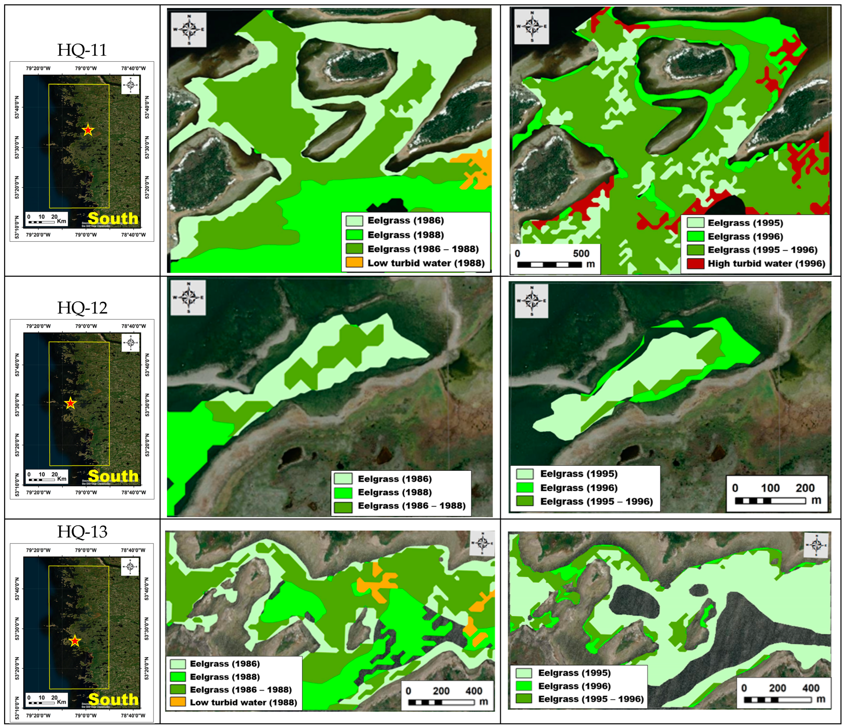
HQ-11	78°59′09″	53°34′27″
HQ-12	79°06′34″	53°30′34″
HQ-13	79°04′35″	53°27′04″

. Each photograph was annotated with the continuous and discontinuous eelgrass distribution limit for each site. These annotated aerial photographs correspond to field surveys from 1986 and 1995, so the classifications from 1988 and 1996 were compared to these photographs. Due to the difference in scale, it was impossible to directly overlay the classified images with a scale of about 1: 30,000 with the HQ eelgrass maps, which have a scale of 1:125,000 (Figure 3). However, for seven sites, we could overlay the limits of eelgrass beds extracted from the classified images and from air photo subsets with eelgrass limits, which were published in [30]. These air photos were first digitised and orthorectified, and the limits were overlaid on the classified images. Such an overlay enabled us to create a map having three classes: (1) areas where the extent of eelgrass agrees between the classified image and the HQ map; (2) areas where eelgrass only exists on the HQ map; and (3) areas where eelgrass only appears on the classified image. This comparison was used to visually evaluate the accuracy of the maps produced by the classification of Landsat imagery at a fine resolution.

3. Results

3.1. Spectral Separability between Classes

Spectral separability between classes varied widely between years, with an average of 1.982 (

Table 6. Class spectral separability assessed using Jeffries-Matusita (J-M) distances calculated using the combination of Landsat spectral bands for each sensor (list of these bands is found in Table 2). J-M distance values range from 0 to 2, 2 representing perfect class separability.

Year	Average	Class	Eelgrass	Low Turbid	High Turbid	Seafloor
1988	1.950	Low Turbid	1.936
		High Turbid	1.901	1.923
		Seafloor	1.974	1.981	1.968
		Deep Water	1.980	1.906	1.931	1.998
1991	1.983	Class	Eelgrass	Low Turbid	High Turbid	Seafloor
		Low Turbid	2.000
		High Turbid	1.966	1.999
		Seafloor	2.000	2.000	2.000
		Deep Water	1.987	1.904	1.979	2.000
1996	1.996	Class	Eelgrass	Low Turbid	High Turbid	Seafloor
		Low Turbid	2.000
		High Turbid	1.997	2.000
		Seafloor	1.994	2.000	1.996
		Deep Water	1.999	1.992	1.986	2.000
2019	1.997	Class	Eelgrass	Low Turbid	High Turbid	Seafloor
		Low Turbid	2.000
		High Turbid	1.999	2.000
		Seafloor	2.000	2.000	1.999
		Deep Water	1.999	1.984	1.985	2.000
Average	1.982	Class	Eelgrass	Low Turbid	High Turbid	Seafloor
		Low Turbid	1.999
		High Turbid	1.999	1.999
		Seafloor	1.999	1.999	1.991
		Deep Water	1.999	1.946	1.970	1.999

), with 2 representing a perfect measure of class separability and 0 representing a complete lack of class separability. Separability between eelgrass and bare seafloor was the highest of all the class pairs, averaging 1.992 across the four classification years. Low turbidity and Deep water were the classes with the lowest average separability (1.946) when averaging over the four years. They had the lowest separability between class pairs in three of the four years. Compared to the average separability across the years, the 1996 and 2019 Landsat images showed the highest average class spectral separability between all spectral class pairs. These two years also showed excellent separability between the eelgrass classes and all other class pairs, with an average separability between eelgrass and all other classes of 1.996 and 1.999 for 1996 and 2019, respectively. The 1988 classification showed the worst average separation between eelgrass and the other class pairs evaluated, consistent with this year having the lowest overall separability between all the evaluated training class pairs.

The spectral reflectance curves confirm the good spectral separability between all the water classes defined with the training areas as a function of the Landsat bands (Figure 7). According to the spectral response recorded by the training areas, all the classes exhibit a general trend that matches how we would expect the light to be absorbed in water, with a stronger reflectance in the green band, which gradually becomes weaker in the longer wavelengths, due to the high absorption by water. This curve also shows that eelgrass detection in water is ensured by a difference in the reflectance value from the vegetation class compared to achlorophyllous classes, such as turbid water, seafloor, and deep water. The spectral reflectance curves also show that the reflectance increases with turbidity, as observed in [127]. However, because the spectral signature of the “High Turbid” class has the strongest reflectance values, eelgrass growing underwater may not be detectable due to the abundance of suspended particles in the water column.

3.2. Image Classification

The overall accuracies of each respective image classification displayed in Figure 8 varied between 94.51% for the 1996 classification and 99.85% for the 2019 classification (

Table 7. Confusion matrices (in number of pixels) and associated classification accuracies for each classification year produced by the RF classifier.

1988	Eelgrass	Low Turbidity	High Turbidity	Seafloor	Deep Water	Total	UA * (%)
Eelgrass	4142	40	15	35	354	4586	90.32
Low Turbidity	68	9041	10	24	81	9224	98.02
High Turbidity	14	8	1859	1	69	1951	95.28
Seafloor	36	15	3	2620	4	2678	97.83
Deep Water	239	25	26	2	119,499	119,791	99.76
Total	4499	9129	1913	2682	120,007	138,230
PA * (%)	92.06	99.04	97.18	97.69	99.58	Overall Accuracy (%) = 99.23
1991	Eelgrass	Low Turbidity	High Turbidity	Seafloor	Deep Water	Total	UA (%)
Eelgrass	2881	15	10	19	103	3028	95.15
Low Turbidity	27	37,016	3	23	1431	38,500	96.15
High Turbidity	14	5	361	2	35	417	86.57
Seafloor	15	45	0	974	0	1034	94.20
Deep Water	26	1335	10	0	54,651	56,022	97.55
Total	2963	38,416	384	1018	56,220	99,001
PA (%)	97.23	96.36	94.01	95.68	97.21	Overall Accuracy (%) = 96.85
1996	Eelgrass	Low Turbidity	High Turbidity	Seafloor	Deep Water	Total	UA (%)
Eelgrass	3367	0	136	58	450	4011	83.94
Low Turbidity	0	12,240	0	0	2323	14,563	84.05
High Turbidity	146	5	3385	45	160	3741	90.48
Seafloor	71	0	31	1624	0	1726	94.09
Deep Water	187	2031	65	0	77,617	79,900	97.14
Total	3771	14,276	3617	1727	80,550	103,941
PA (%)	89.29	85.74	93.59	94.04	96.36	Overall Accuracy (%) = 94.51
2019	Eelgrass	Low Turbidity	High Turbidity	Seafloor	Deep Water	Total	UA (%)
Eelgrass	12,906	0	0	1	25	12,932	99.80
Low Turbidity	0	31,055	1	0	178	31,234	99.43
High Turbidity	1	1	9674	0	300	9976	96.97
Seafloor	0	0	0	3618	0	3618	100.00
Deep Water	4	175	3	0	414,701	414,883	99.96
Total	12,911	31,231	9678	3619	415,200	472,643
PA (%)	99.95	99.44	99.96	99.97	99.88	Overall Accuracy (%) = 99.85

(*) Bold figures indicated well-classified pixels; PA = producer’s accuracy; UA = user’s accuracy.

). Producer’s accuracies for the “eelgrass” class were the lowest for the 1996 classification (89.29%) and the highest for the 2019 classification (99.95%). By all three metrics stated, the 2019 classification using Landsat-8 imagery was the most accurate of the four classified images, and the 1996 classification (Landsat-5) was the least accurate.

RF produces a list of variables used according to their order of importance (

Table 8. The order of importance of each input feature ranked from the most (1) to the least important (24) as a function of the classification year. The top 10 most important input features are bolded.

Layer	1988	1991	1996	2019
Coastal	n.d.	n.d.	n.d.	3
Blue	11	2	18	6
Green	3	1	4	4
Red	8	10	6	13
NIR	5	4	5	14
SWIR-1	18	18	21	2
SWIR-2	4	21	22	25
Turbidity	7	9	10	1
Bathy-BG	10	8	9	7
Bathy-CG	n.d.	n.d.	n.d.	9
Bathy-BR	12	5	7	19
Bathy-CR	n.d.	n.d.	n.d.	17
DVI	13	12	8	15
GDVI	9	3	3	5
GNDVI	20	16	13	23
GRVI	21	15	16	21
NDAVI	15	14	11	11
NDVI	19	20	15	20
NG	16	7	14	12
NNIR	22	17	19	18
NR	14	13	20	16
RVI	17	19	12	24
WAVI	6	11	17	10
RD-1	2	6	1	8
RD-2	1	22	2	22

). Like [50,54,105], we found that the green reflectance band was among the most important in every image classification, particularly for the 1991 classification, mostly because this band has better penetration in water [128,129,130] and is more sensitive to the green vegetation found near the water surface [54,105,130,131,132]. The other visible bands (red and blue) are also among the most important, with the coastal band in the Landsat-8 OLI satellite image, because the wavelengths associated with these bands can penetrate more deeply through the water. While near-infrared radiation is expected to be readily absorbed by water [98], the NIR reflectance band is among the ten most important variables in the classification of the Landsat-5 TM images, likely indicating that eelgrass plants are found in very shallow water [129,133,134]. Because they do not penetrate water as well due to their longer wavelength [128], the shortwave infrared bands (SWIR-1 and SWIR-2) are less important, as shown by the reflectance values used to draw the curves (Figure 7). The turbidity layer produced with ACOLITE was also important for all the classified images (Table 8), particularly for the 2019 classified image, as the waters of James Bay were particularly murky during that year [107]. Although eelgrass is a chlorophyllous feature, the vegetation indices were generally less important than the original bands of reflectance, except for the Green Difference Vegetation Index (GDVI), which is based on the reflectance of the two spectral bands that are the most sensitive to the presence of vegetation, namely the green and the NIR spectral bands (Table 3). Finally, among all bathymetric variables used in RF, the Relative Depth-1 (RD-1) and the blue/green ratio are always among the top 10 most important variables in all the classification of Landsat imagery. The Relative-Depth 1 (RD-1) variable seems very important, even if the water could be murky.

3.3. Validation of the Image Classification

The validation of classified images is based on two methods. The first method assesses each classified image with observation sites (eelgrass present/absent) derived from historical Hydro-Québec (HQ) eelgrass distribution maps for 1986, 1991, and 1995, as well as the James Bay Comprehensive Coastal Assessment Program (JBCCAP) team’s field validation set for the 2019 classification. The results are displayed as a confusion matrix for each classified image (

Table 9. Confusion matrices related to the validation accuracy determined by comparing the classified image to a dataset different from the one used for the training areas for each classification year.

		Ground-Truth
1988	Class	Eelgrass present	Eelgrass absent	Total	UA * (%)
Classified	Eelgrass Present	42	11	53	79.3
	Eelgrass Absent	8	62	70	88.6
	Total	50	73	123
	PA * (%)	84.0	84.9	Overall Accuracy (%) = 84.6
		Ground-Truth
1991	Class	Eelgrass Present	Eelgrass Absent	Total	UA * (%)
Classified	Eelgrass Present	75	16	91	82.4
	Eelgrass Absent	25	84	109	77.1
	Total	100	100	200
	PA * (%)	75.0	84.0	Overall Accuracy (%) = 79.5
		Ground-Truth
1996	Class	Eelgrass Present	Eelgrass Absent	Total	UA* (%)
Classified	Eelgrass Present	66	12	78	84.6
	Eelgrass Absent	24	78	102	76.5
	Total	90	90	180
	PA * (%)	73.3	86.7	Overall Accuracy (%) = 80.0
		Ground-Truth
2019	Class	Eelgrass Present	Eelgrass Absent	Total	UA * (%)
Classified	Eelgrass Present	69	13	82	84.2
	Eelgrass Absent	10	16	26	61.5
	Total	79	29	108
	PA * (%)	87.3	55.2	Overall Accuracy (%) = 78.7

(*) Bold figures indicated well-classified sites; EC = error of commission; EO = error of omission; PA = producer’s accuracy; UA = user’s accuracy.

). The overall validation accuracy was the highest for the 1988 classification (84.5%) and the lowest for the 2019 classification (74.5%). Producer’s accuracies of the eelgrass present class ranged from 73.3% with the 1996 classification to 84.0% with the 1988 classification, while the corresponding user’s accuracies ranged from 79.2% with the 1988 classification to 91.1% with the 2019 classification, indicating reasonable consistency between classification results. The 1988 (123 sites) and 2019 (128 sites) classifications had significantly fewer validation sites compared to the 1991 (200 sites) and 1996 (180 sites) classifications due to the lower availability of data for 1988 and 2019. In the case of the classified image for 2019, the lower number of sites for validation is mostly related to the turbidity of the coastal water of James Bay at several validation sites [107].

The second method validated the results at a finer resolution than at the bay scale by comparing the classified images with maps produced for seven sites selected from the studies carried out on behalf of HQ (Table 5). Since aerial photographs were unavailable for 1991, only the 1988 and 1996 classifications were compared at individual HQ sites where eelgrass beds were manually digitalised (Figure 9). There are some agreements concerning eelgrass presence between both types of maps in most sites, but the boundaries and extents are different. Generally, the edges of the eelgrass meadows did not perfectly match the classified images and the air photo interpretations, probably because of a difference in the scale of the original dataset (1:30,000 for the image versus 1:10,000 for aerial photographs). It should be noted that, on the 1988 classified image, eelgrass occupied more area in all sites and was found further offshore, compared to the areas mapped on the 1986 aerial photos. On the opposite, the eelgrass delineated on the 1996 classified image generally extends closer to the coast if we compare it with the limits of eelgrass on the aerial photos dating from 1995. Finally, on the 1996 classified image for several sites, i.e., HQ-08, HQ-09, HQ-12, and HQ-13, the extent detected from the Landsat imagery covers a much smaller area than that established from the 1995 aerial survey (Figure 9).

3.4. Temporal Evolution of the Eelgrass Extent

The area of eelgrass beds mapped with the classified images over each zone was quantified (

Table 10. The surface (in km²) covered by eelgrass beds in the two AOIs, according to previous studies and this study.

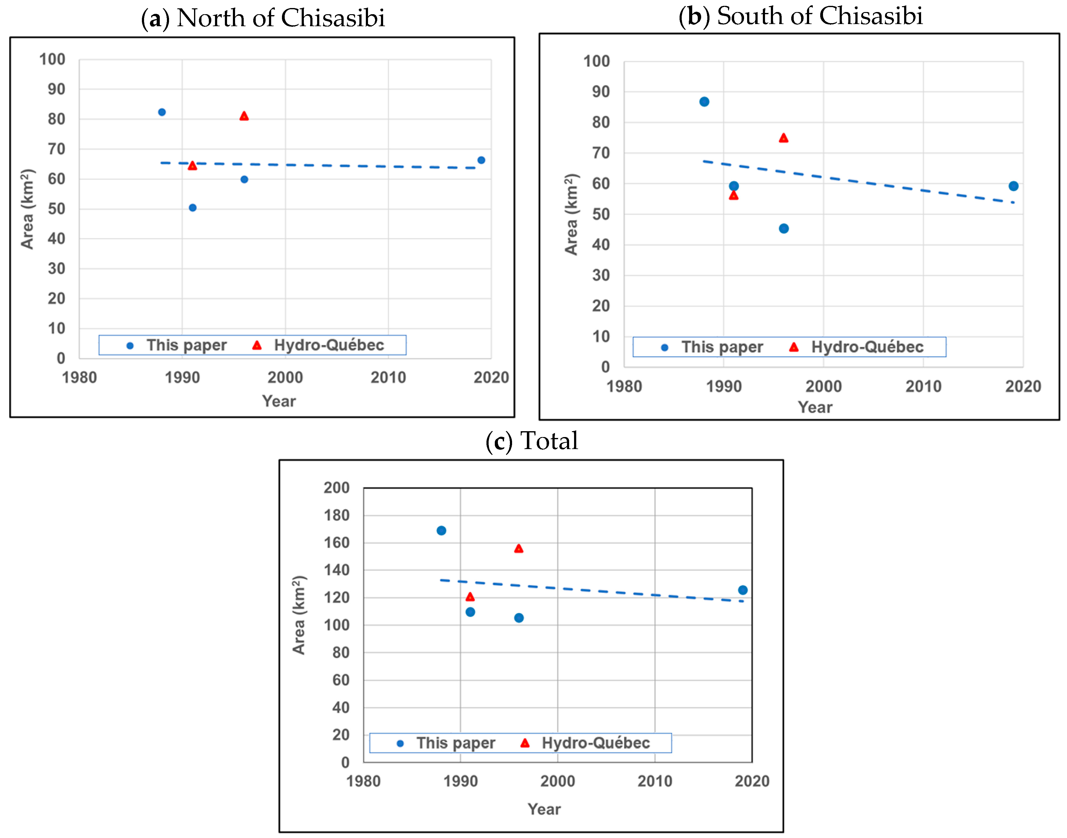
Year	North	South	Total	Source
1986	79.61	n.d. *	93.02	[43]
1988	82.39	86.89	169.28	This paper
1991	64.56	56.34	120.90	[45]
1991	50.47	59.35	109.82	This paper
1995	81.19	74.97	156.16	[40]
1996	60.00	45.51	105.51	This paper
2019	66.37	59.31	125.68	This paper

* The 1986 map of eelgrass only covers a small part of the AOI located south of Chisasibi; therefore, the total measured area is not considered in this study.

) and plotted (Figure 10). This figure shows a declining trend in eelgrass extent observed throughout the study period for both AOIs and the total study period. However, the 2019 extent was slightly higher than the 1991 and 1996 extents. The areas covered by eelgrass mapped by Hydro-Québec in 1991 and 1996 are also shown. The classified image area compares well with the Hydro-Québec area in 1991 for the south of Chisasibi AOI but not for the north of Chisasibi AOI. The difference was the most important for the 1996 classification.

4. Discussion

4.1. An Assessment of the Classified Images

The overall classification accuracy of our classified Landsat imagery assessed by comparing with the training data subset ranged from 94.51% for the 1996 classification to 99.85% for the 2019 classification (Table 7), indicating exceptionally high classification accuracies for all the years. The quality of the training areas can first explain these good results. Indeed, all the training areas for the “Eelgrass” class have a good spectral separability between classes, with a J-M distance greater than 1.9 from the other classes, whatever the year (Table 6). The good spectral separability of eelgrass from other unvegetated classes is also shown in the graphical representation of the class spectral response for each Landsat band (Figure 7). For the “Eelgrass” class, the spectral signature is in agreement with the one obtained in other studies [130,131], with the highest reflectance in the green band [4,132,135]. Figure 7 also shows that the “High Turbid Water” class has the highest reflectance value in all the bands, such as a terrestrial class. In addition, the spectral separability between “Deep Water” and shallower “Eelgrass” is obvious in the case of clear water but not when the water is murky or coloured.

The comparison with the validation datasets led to accuracies for eelgrass presence/absence ranging between 78.7% for the 2019 classification and 84.6% for the 1988 classification (Table 9). These validation accuracies are lower than the classification accuracies extracted from image data. In addition, the validation accuracies were established with a lower number of data than the classification accuracies. Also, there were some year differences between the image dates and the time when the validation data were collected. However, our validation accuracies are better than those obtained in previous studies on eelgrass bed mapping along the eastern part of James Bay. With the Maximum Likelihood Classifier (MLC), an accuracy of 73.7% was achieved when using PlanetScope images [64] and 75.6% when using PlanetScope, Worldview-2, and RapidEye-5 images [19]. The authors of ref. [63] obtained an accuracy of 72.7% when applying an unsupervised IsoCluster classifier to Worldview-2 and RapidEye-5 images. These lower accuracies can be explained by (1) the use of classifiers that were already shown to be less efficient than the RF classifier we used [65,66,67,68]; (2) the fact that the input features did not have shortwave infrared bands nor green-based vegetation indices, such as the GDVI, both being among the most important variables in our classification (Table 8); and (3) the studies did not consider bathymetric data or their proxies such as the bathymetric ratios and relative depth layers we used in our study. Similarly, our overall validation accuracies were slightly greater than those [136] (72%) who mapped the presence/absence of eelgrass beds in Greece using Sentinel-2 imagery and a Support Vector Machine classification via Google Earth Engine. Our results were comparable and, in some instances, better than those using Sentinel-2 imagery for mapping eelgrass along Canada’s Atlantic coast, such as [50] (78%) with Random Forests and [137] (79%) with a hierarchical classifier. On the west coast of Canada, eelgrass classification studies by [131] showed accuracies of 83% with AISA hyperspectral imagery and 68% with IKONOS high-resolution imagery. In [138], the authors obtained an accuracy of 75% with WorldView-2 imagery.

The classification analysis determined the best image features to distinguish eelgrass from other underwater classes. The green band reflectance consistently emerged as one of the most important input features to produce a classified image with the RF classifier (Table 8). It effectively distinguishes eelgrass from the other classes in the spectral signature plot (Figure 7), a result that aligns with [54]. The importance of the green band reflectance can be attributed to its deeper penetration in water [4,128,130] and the high reflectance due to the red and blue reflectance absorption by the eelgrass chlorophyll [4,54,105,129,130,131,132,135]. This is why a strong green hue expresses the reflectance of submerged eelgrass in Landsat RGB imagery, which helps to delineate training areas associated with the eelgrass class. The vegetation indices were generally less important than the simple band reflectance (Table 8), except for the Green Difference Vegetation Index (GDVI), which includes the green band reflectance (Table 3). The red or near-infrared band reflectance was not as useful for detecting eelgrass in the AOIs despite their sensitivity to chlorophyll [50,54,129,133,134]. Indeed, the radiation in these bands is highly absorbed by the water [4,51,130,135].

Our study also showed that adding bathymetric variables to the classification helped to detect eelgrass beds by delineating areas where the depth is appropriate for eelgrass. Among all bathymetric data used in the classification, the blue/green ratio and the Relative Depth-1 (RD-1) variable were always among the top 10 most important input features (Table 8). The blue/green ratio is computed with the blue and green band reflectance [105,132] that was already shown to be very useful in detecting eelgrass beds. The Relative Depth-1 (RD-1) variable allows us to locate areas that have a depth of less than 2 m, which is suitable for eelgrass growth even in the case of turbid water. The Relative Depth-2 (RD-2) variable (depths between 2 and 5 m) is also important for two classification years (1988 and 1996), which corresponded to years with less murky water influence.

4.2. Eelgrass Spatial and Temporal Dynamics

As in the historical maps (Figure 3), our classified images showed that eelgrass beds are mostly found inside sheltered embayments in the two AOIs (Figure 8). The areas extracted from the historical maps and the classified images are very similar in 1988 and 1991, but only for the south AOI, but not in 1996 (Table 10). For both methods, there were inaccuracies associated with the environmental conditions during the data acquisition. For the aerial photograph-based methods, waves or sun glint did not allow us to see the underwater eelgrass beds well either on the aerial photo or from the helicopter [43]. Another problem with the method was that some observations were made without considering the tidal height, as in 1986 [59,60] and 1995 [30]. However, this method better considers the water turbidity as the aerial photographs or helicopter surveys were conducted over several weeks, which allowed us to obtain the most optimal condition concerning this factor. Sun glint was not an issue for the Landsat-based method because of the ACOLITE correction. However, there was significant water turbidity on the images that precluded the detection of some portions of the eelgrass beds, thus possibly leading to eelgrass areas smaller than the actual ones. Tide height is also an important factor to be considered. It was impossible to assess the tidal height’s effect on the measured total area covered by eelgrass due to the lack of tidal measurements. However, the visual inspection of the Landsat images shows that some images were acquired at high tides. This was probably the case for the 1996 image and could be one of the reasons why the total area of eelgrass extracted from the 1996 classified image appears considerably lower than in other classification years.

There is an additional source of inaccuracy related to the aerial photo-based method that differed as a function of the year. The eelgrass map published in 1988 [59] is based on a manual delineation of eelgrass beds over a 1:50,000 topographic map during low-level, slow-speed helicopter flights along the coast. After, these delineations were transferred to 1:10,000 aerial photographs [23,59,61]. In the case of the 1996 eelgrass map [30], the delineation was conducted by the photointerpretation of 1:10,000 colour aerial photographs acquired at low tide in August 1995 and validated in the field in 1996 [23]. In both cases, the resulting maps were at a scale of 1:125,000 [30,59,61], even if the aerial photographs were at a 1:10,000 scale [23,30,59,139]. Such a scale change resulted in some inaccuracies due to the generalisation of the limits of the eelgrass beds [20]. In addition, the 1:125,000 maps did not capture the fine details of the rugged coastline of eastern James Bay [59], which can lead to additional inaccuracies. All the delineations of the eelgrass beds were conducted manually with a pen, and an error of 1 mm in the position induces an error of 125 m on the 1:125,000 maps.

Despite the possible inaccuracies associated with both methods, the extracted areas allow us to assess the evolution in the extent of eelgrass over time (Figure 10). It is impossible to compute regression models due to the lack of a suitable number of data, particularly for the 1996–2019 period, given no historical data were available to validate any classified images. We also did not consider the period before 1985, i.e., before the development of the La Grande Hydroelectric Complex, because of the absence of suitable multispectral optical imagery. Figure 10 shows a decline in eelgrass bed areas before 2000, consistent with the documented Cree observations [140] and the investigations led by the team of the CHCRP [16]. Such a decrease in eelgrass beds in the coastal waters of James Bay was also observed at the bay level for the 1986–1988 and 1995–1996 periods (Figure 9).

Comparing the maps produced from aerial photos with the classified images at the site level shows that the eelgrass beds covered a similar area (displayed in dark green in Figure 9) for the HQ-10 and HQ-11 sites for both periods, for HQ-07 only for the 1995–1996 period, and for HQ-08 and HQ-13 but only for the 1986–1988 period. However, it seems that the 1988 Landsat imagery detects eelgrass beds located more offshore than in 1986 for all the sites. This agrees with the observations of [23,30,59] who explained this local migration of eelgrass beds offshore due to the glacio-isostatic rebound. Indeed, given the very low slope of the seafloor in the embayments of 0.5 m/km [28] and a rate of glacio-isostatic recovery of approximately 1 cm/year [83], we can estimate a retreat of the coast of 20 m between the two years, which agrees with the estimate already made [30]. However, the eelgrass beds are closer to the coast on the 1996 classified image compared to the 1995 aerial photographs. The high tide associated with the 1996 image could explain such a change.

4.3. Sources of Water Turbidity

Water turbidity is another problem in detecting eelgrass beds in the coastal waters of eastern James Bay. Water turbidity is due to suspended matter in the water column [44,141,142]. The suspended matter includes sediments, mainly silt, and colloidal materials, such as clay and organic matter [20,141,142,143]. Low suspended matter concentrations are mainly made of colloids, which colour the water [19,20,143]. The amber orange colour of the water is due to the Coloured Dissolved Organic Matter (CDOM), while the greyish colour is due to clay [26,106]. In both cases, the reflectance coming from the seabed is distorted [34], leading to a possible misclassification of the true extent of eelgrass meadows [48,64]. When the concentration of suspended matter is high, it is because of the presence of sediments (mainly silt) in addition to colloidal materials, and the water becomes very murky and opaque, making it impossible to detect what is on the seafloor [127,144]. Our Landsat-classified images show that water turbidity was found at several embayments along the coast of both AOIs whatever the year (Figure 8). Indeed, on each image, some areas had coloured or cloudy water, which precludes determining whether the seabed was covered or not with eelgrass. The water turbidity was variable spatially as a function of the year, which could be one of the causes for the differences in the areas covered by eelgrass beds for the same or close years compared to the aerial photograph-based mapping (Table 9 and Figure 10). The presence of turbid water in the two AOIs is in agreement with the observations made by many previous studies on mapping eelgrass beds in James Bay from aerial photographs [23,30,59,72,88,139,145], helicopter flights [30,59,61,72,88,139,146], diving [20,23,30,33,59,61,72,139,145], or satellite image classification [19,63,64,107]. This is also in agreement with the observations of the Cree land users of Eeyou Istchee, who already reported increasing turbidity in the water along the eastern coast of James Bay from the mid-1980s, with a peak in the 1990s [18,19,20,140,147,148].

As shown in Figure 8, the major source of water turbidity is the freshwater flume of rivers entering James Bay, which spread northwards along the eastern shore of James Bay because of drift currents moving along the coast. Indeed, James Bay water has a cyclonic circulation [19,85,149] that follows a counterclockwise gyre [73,84,86]. The turbidity at the mouth of the rivers is often used as one of the potential causes to explain the lack of eelgrass in river estuaries [19,145]. This is the case for the La Grande River [27], which naturally has murky water [25,150,151] because of the bank erosion of the sandy island at the mouth of the river [31] and the easily erodible marine clays and glacial till outcrops further upstream [31,150,152]. The river became even murkier with the development of the hydroelectric complex on the La Grande River [19,20,140]. The riverbanks also experienced numerous landslides because of their nature [152,153,154,155,156]. This was the case in 1987, after the La Grande Hydroelectric Complex was completed but before its commissioning [157].

Figure 8 shows rivers other than La Grande and Eastmain rivers having a turbid water discharge in James Bay. This observation agrees with past observations made by several studies and by local people [19,20,22,25,32,57,61,87,107,147,149,150,154]. However, the turbidity was sporadic but not constant [20,23,33,61,107]. As mentioned earlier, the studies could not determine whether the variation in the water turbidity was seasonal and linked to periods of high flow, given that all the observations were made in late summer when the eelgrass was in full bloom. Given that these rivers were not subjected to hydroelectric developments, there is a need to investigate the source of the water turbidity further. As shown by [158] with the Landsat imagery series acquired over the 2013 megafire in the Eastmain River watershed, forest fires can also be a source of water turbidity. Indeed, Eeyou Istchee is a region prone to forest fires [159,160,161,162], mainly because of the vegetation cover type [163,164]. In addition to large patches of old coniferous trees developed in a boreal climate [165,166], peatlands are abundant, covering up to 20% of the landscape [163]. Under dry, warm, and windy conditions, peat is vulnerable to intense burning [163,164,167,168,169,170], especially when a thick sphagnum peat moss cover is present at the surface of raised bogs [164,171,172] and the water table is low during periods of drought [172]. Lightning can easily ignite this organic material, while sustained windy and dry weather can encourage the spread of large fires [173] across relatively flat topography [162,174]. When a layer of organic soil ignites, the peat can burn deeper into the soil, often without a flame, so plant roots are killed, leading to the disintegration of the surface and the formation of more easily mobilised particles, especially unconsolidated light powdery ash [175,176]. After the wildfire is extinguished, the erosion of the exposed combusted peat is accelerated in burnt areas by rain, which is not intercepted because of the absence of living vegetation [177] and by the transport of DOC by the runoff [175,178,179,180]. Rapid erosion in the most severely burnt zone results in a very high export of DOC from the peat bogs and increased suspended sediment loads in watercourses [175,176,177]. This contribution of suspended debris could explain the high level of dissolved organic carbon (DOC) in the coastal waters of James Bay, as already observed in situ [19,23,149], as well as the orange or amber colour of the water found in some embayments [19,20,63,64], after the deposition of suspended mineral particles.

Figure 11 presents the change in the area affected by forest fires in the James Bay watershed of Quebec, extracted from the Forest Fire database produced by the Quebec Ministry of Forests, Wildlife, and Parks [181], as a function of the year of the event. These compiled data about the burned area in Eeyou Istchee are very similar to the trends obtained for the Hudson Plains Ecozone [165,182] and the province of Quebec [183], according to the Canadian National Fire Database [184]. Most of these wildfires were natural due to lightning during thunderstorms, particularly the largest ones [165,181,182]. The plot of Figure 11 shows that, in addition to the 2013 Eastmain megafire, the peak of burned areas occurred in 1989 in the James Bay watersheds of Quebec. Indeed, 1989 was a particularly catastrophic year for Canada’s forests, with some of the largest areas burned since the 1960s [165,166,182,185,186]. Covering a total surface of about 19,755 km² in the James Bay watersheds of Quebec, three megafires were located on lands east of the Eeyou communities of Chisasibi and Wemindji (Figure 12). Part of the 1989 burnt areas in the Eastmain region were re-burned in 2013 [163,184,186]. As shown in Figure 13, comparing Landsat-TM images acquired before and after the 1989 wildfires, river water turbidity significantly increased in several rivers flowing into James Bay after the 1989 megafires, even in the case of rivers without hydroelectric complexes or other manmade features. As in the case of the Eastmain River and the 2013 megafire [158], all these rivers became murky after flowing through burn scars because of post-fire erosion that produced suspended matter. The effect of burn scars on the water turbidity can still be visible longer after the event, as shown by the oblique air photo acquired in 2022 over the Sculpin River that runs through the 2013 Eastmain fire scar (Figure 14).

4.4. Issues in Eelgrass Mapping

This study was limited by multiple factors, including the availability of suitable ice- and cloud-free imagery covering the whole study area and the correct temporal period, tidal differences between images, limited spatial resolution, and the quality of available ground truth data. The imagery classified in this present study was acquired after the completion of most of the La Grande Hydroelectric Complex, making it difficult to determine the potential effects of the hydroelectric project on eelgrass distribution in the bay. Even though historical data exist from before the complex’s construction [57,58], there is no multispectral satellite imagery from the Landsat collection to perform this analysis. In addition, some of the images acquired (i.e., 1988 and 1996) were acquired within two years of the data collected and published by Hydro-Québec, limiting the precision with which we can compare our image classifications to preexisting historical data. Since cloud- and ice-free imagery covering the full extent of the Eeyou Istchee coastline are scarce, tidal differences between images, which can affect the depth at which eelgrass can be detected, are reluctantly apparent between the three historical image classifications (as documented by the total number of water pixels in each image). This difference likely affects the extent to which the Landsat sensor can detect eelgrass, as eelgrass extent can be measured further out when the tidal level is lower because there is less water column above the eelgrass to obfuscate the reflectance signal. This factor, therefore, presents a possible explanation as to why the extent of the classified eelgrass beds in 1996 was the lowest. However, without reliable tidal data, it is impossible to estimate the exact effect of tidal differences in determining the classified eelgrass area. Ideally, imagery acquired at the lowest possible tidal level should be prioritised when detecting submerged aquatic vegetation.

While effective for change detection in large areas, Landsat-derived image classifications have many limitations on their applicability. Moderate spatial resolution presents an advantage in covering a large aerial swath. However, mapping accuracy comes at a cost compared to utilising imagery with higher spatial resolutions. Large eelgrass beds, mainly when a SIEVE filter was applied to the classified images, were easily detectable, and their general shape and distribution were monitorable. The SIEVE filter helped remove erroneously classified eelgrass pixels located in deep water. For a pixel to be classified as eelgrass, submerged aquatic vegetation should be the dominant reflectance signal in the area covered by the pixel (900 m²). Therefore, this approach cannot accurately reflect smaller eelgrass beds because of possible confusion with other features. Also, there could be possible confusion with other subaquatic vegetation types that are not eelgrass since our classification method has only one class for the subaquatic vegetation. While eelgrass is the dominant submerged vegetation across the eastern coast of James Bay, more localised populations of Ruppia maritima, Ascophyllum nodosa, or Fucus vesiculosus were also shown to be present [59,88]. They could also be misinterpreted as eelgrass when examining aerial photographs or classifying a satellite image. Such a limitation outlines the need for diver-led field verification to assess the various types of submerged aquatic vegetation and their distribution within the study area [19,59].

5. Conclusions

Our Landsat image classifications displayed the ability to map large eelgrass beds in James Bay with relatively strong accuracy on a large scale. They accurately captured the presence and the extent of eelgrass beds at a relative scale of approximately 1:10,000 (dependent on the year and environmental factors, including water turbidity and tidal level). Our classification accuracies, assessed using a subset of the training data and an independently generated ground-truth dataset, achieved comparable or better overall accuracies than other studies utilising multispectral image classifications to map seagrasses in turbid northern waters (including studies using higher-resolution imagery such as [63,64]). The methodology we tested in our study is a reasonably cost-effective way to monitor eelgrass beds in James Bay temporally. The total costs associated with this mapping approach were kept low by utilising publicly available imagery and free, open-source atmospheric correction software, which limited the project’s cost to the time required to perform and analyse the classified imagery and the fieldwork necessary to ground the truth of the classification. Temporal trends exhibited in our study showed a decrease in the total extent of eelgrass classified over the studied period, which is consistent with observations made by local people. The losses and gains for each zone evaluated can be attributed mainly to a few large eelgrass areas.

Since eelgrass growth is limited by light availability [186,187], water depth can be a major factor in determining the development of eelgrass beds in turbid water such as the one of James Bay. Given that James Bay has no accurate bathymetric data, the bathymetry was considered by adding two “relative depths” and “bathymetric ratios” to the classification to exclude areas where eelgrass could not grow because the water was too deep. Further work is needed to test actual bathymetry data in the classification. Eelgrass is also sensitive to other environmental factors such as salinity and substrate type. It is necessary to add these variables to the classification method. Another factor that can limit the availability of light for eelgrass is water turbidity, which makes it an important environmental parameter to monitor in James Bay. We showed that the 1989 wildfires influenced the turbidity of the rivers flowing to the bay, but further research should be carried out to investigate more in detail the effects of wildfire on bay-wide turbidity and, further, how changes in water turbidity affect the health and distribution of eelgrass in James Bay.

Overall, this study showed that multispectral image classification could be a valuable tool for detecting and mapping large eelgrass beds along the eastern coast of James Bay, even in locations with variably turbid water. Our study also showed that satellite image analysis offers a unique ability to evaluate data retroactively and in real time, which can be a precious tool for looking at temporal change analysis. Indeed, the Landsat archive is continuously and consistently updated within the USGS database, giving this type of study widespread applicability for past and future change detection analysis. Multispectral image classification can be used independently but is best used with one or multiple field surveys or other datasets. The resulting classified image maps can and should be used to inform and guide future studies on where eelgrass distribution might be changing or should be monitored, such as in the case of the eastern coastline of James Bay.

References

- Nienhuis, P.; Groenendijk, A. Consumption of eelgrass (Zostera marina) by birds and invertebrates: An annual budget. Mar. Ecol. Prog. Ser. 1986, 29, 29–35. [Google Scholar] [CrossRef]
- Kennedy, L.A.; Juanes, F.; El-Sabaawi, R. Eelgrass as valuable nearshore foraging habitat for juvenile Pacific Salmon in the early marine period. Mar. Coast. Fish. 2018, 10, 190–203. [Google Scholar] [CrossRef]
- Wong, M.C.; Bravo, M.A.; Dowd, M. Ecological dynamics of Zostera marina (Eelgrass) in three adjacent bays in Atlantic Canada. Bot. Mar. 2013, 56, 413–424. [Google Scholar] [CrossRef]
- Komatsu, T.; Hashim, M.; Nurdin, N.; Noiraksar, T.; Prathep, A.; Stankovic, M.; Hoang Son, T.P.; Minh Thu, P.; Luong, C.V.; Wouthyzen, S.; et al. Practical mapping methods of seagrass beds by satellite remote sensing and ground truthing. Coast. Mar. Sci. 2020, 43, 1–25. [Google Scholar] [CrossRef]
- Heck, K.L.; Able, K.W.; Roman, C.T.; Fahay, M.P. Composition, abundance, biomass, and production of macrofauna in a New England estuary: Comparisons among eelgrass meadows and other nursery habitats. Estuaries 1995, 18, 379–389. [Google Scholar] [CrossRef]
- Nahirnick, N.; Costa, M.; Schroeder, S.; Sharma, T. Long-term eelgrass habitat change and associated human impacts on the West Coast of Canada. J. Coast. Res. 2020, 36, 30–40. [Google Scholar] [CrossRef]
- Kollars, N.M.; Henry, A.K.; Whalen, M.A.; Boyer, K.E.; Cusson, M.; Eklöf, J.S.; Hereu, C.M.; Jorgensen, P.; Kiriakopolos, S.L.; Reynolds, P.L. Meta-analysis of reciprocal linkages between temperate seagrasses and waterfowl with implications for conservation. Front. Plant Sci. 2017, 8, 2119. [Google Scholar] [CrossRef] [PubMed]
- Ward, D.H.; Markon, C.J.; Douglas, D.C. Distribution and stability of eelgrass beds at Izembek Lagoon, Alaska. Aquat. Bot. 1997, 58, 229–240. [Google Scholar] [CrossRef]
- Jeffery, N.; Vercaemer, N.; Stanley, R.; Kess, T.; Dufresne, F.; Wong, M. Variation in genomic vulnerability to climate change across temperate populations of eelgrass (Zostera marina). Evol Appl 2024, 17, e13671. [Google Scholar] [CrossRef]
- Short, F.; Wyllie-Echeverria, S. Natural and human-induced disturbance of seagrasses. Environ. Conserv. 1996, 23, 17–27. [Google Scholar] [CrossRef]
- Morris, C.J.; Gregory, R.S.; Laurel, B.J.; Methven, D.A.; Warren, M.A. Potential Effect of Eelgrass (Zostera marina) Loss on Nearshore Newfoundland Fish Communities, Due to Invasive Green Crab (Carcinus maenas); Research Document 2010/140; DFO Canada Science Advisory Secretariat: Ottawa, ON, Canada, 2011; pp. 1–17. [Google Scholar]
- DFO. Does Eelgrass (Zostera marina L.) Meet the Criteria as an Ecologically Significant Species? Research Document 2009/018; Department of Fisheries and Oceans, Canadian Science Advisory Secretariat: Ottawa, ON, Canada, 2009; pp. 1–10.
- Prevett, J.P.; Lumsden, H.G.; Johnson, F.C. Waterfowl kill by Cree hunters of the Hudson Bay Lowland, Ontario. Arctic 1983, 36, 185–192. [Google Scholar] [CrossRef]
- Royer, M.-J.S. Eastern James Bay and the Cree. In Climate, Environment and Cree Observations: James Bay Territory, Canada; Royer, M.-J.S., Ed.; Springer Briefs in Climate Studies; Springer International Publishing: Cham, Switzerland, 2016; pp. 35–61. ISBN 978-3-319-25181-3. [Google Scholar]
- Rivers, D.O.; Short, F. Effect of grazing by Canada geese Branta Canadensis on an intertidal eelgrass Zostera marina meadow. Mar. Ecol. Prog. Ser. 2007, 333, 271–279. [Google Scholar] [CrossRef]
- Leblanc, M.-L.; O’Connor, M.I.; Kuzyk, Z.Z.A.; Noisette, F.; Davis, K.E.; Rabbitskin, E.; Sam, L.-L.; Neumeier, U.; Costanzo, R.; Ehn, J.K.; et al. Limited recovery following a massive seagrass decline in subarctic eastern Canada. Glob. Change Biol. 2022, 29, 432–450. [Google Scholar] [CrossRef]
- COMEX. Report on the Public Consultations Held in November 2012 Following Implementation of Hydro-Quebec’s Eastmain-1-A and Sarcelle Powerhouses and Rupert Diversion Project; Comité d’examen de la Convention de la Baie-»James et du Nord Québécois: Québec, QC, Canada, 2013; 238p.
- COMEX. Eastmain-1-A and Sarcelle Powerhouses and Rupert Diversion. Followup of Eelgrass Beds on the Northeast Coast of Baie James (James Bay)—Study Report 2014; Comité d’examen de la Convention de la Baie-»James et du Nord Québécois: Québec, QC, Canada, 2017. [Google Scholar]
- Short, F.T.; Torio, D.; Anderson, N. James Bay Eelgrass Project—Final Report; University of New Hampshire: Durham, NH, USA, 2019; 85p. [Google Scholar]
- Kuzyk, Z.A.; Leblanc, M.-L.; O’Connor, M.; Idrobo, J.; Giroux, J.-F.; del Giorgio, P.; Bélanger, S.; Noisette, F.; Fink-Mercier, C.; de Melo, M.; et al. Understanding Shkaapaashkw: Eelgrass Health and Goose Presence in Eastern James Bay; Final Report from the Eeyou Coastal Habitat Comprehensive Research Project (CHCRP); Prepared for Niskamoon Corporation; University of Manitoba: Winnipeg, MB, Canada, 2023; 279p. [Google Scholar] [CrossRef]
- Marsh, J.H. James Bay Project. The Canadian Encyclopedia. 2023. Available online: https://www.thecanadianencyclopedia.ca/en/article/james-bay-project (accessed on 15 February 2023).
- Messier, D.; Ingram, R.G.; Roy, D. Physical and biological modifications in response to La Grande hydroelectric complex. In Canadian Inland Seas; Martini, I.P., Ed.; Elsevier Oceanography Series No. 44; Elsevier: Amsterdam, The Netherlands, 1986; pp. 403–424. [Google Scholar]
- Lalumière, R.; Lemieux, C. Suivi Environnemental des Projets La Grande-2-A et La Grande-1. La Zostère marine de la Côte Nord-est de la Baie James; Rapport Synthèse Pour la Période 1988–2000; Report HQ-2002-100; Groupe Conseil GENIVAR: Québec, QC, Canada, 2002; 92p. [Google Scholar]
- Hydro-Québec Production. La Grande Hydroelectric Complex: 16—Rivers with Modified Flow; Report HQ-ENVI-94-1174; Hydro-Québec Production: Québec, QC, Canada, 2003; 6p. [Google Scholar]
- Reed, A.; Benoît, R.; Lalumière, R.; Julien, M. Duck Use of the Coastal Habitats of Northeast James Bay; Occasional Paper No. 90; Canadian Wildlife Service: Ottawa, ON, Canada, 1991; 47p. [Google Scholar]
- El-Sabh, M.I.; Koutitonsky, V.G. An oceanographic study of James Bay before the completion of the La Grande Hydroelectric Complex. Arctic 1977, 30, 169–186. [Google Scholar] [CrossRef]
- Messier, D. Suivi Environnemental des Projets La Grande-2-A et La Grande-1. Le Panache de La Grande Rivière; Rapport Synthèse Pour la Période 1987–2000; Direction Barrages et Environnement; Report HQ-2002-129; Hydro-Québec Production: Québec, QC, Canada, 2002; 73p. [Google Scholar]
- Martini, I.P. Coastal features of Canadian inland seas. In Canadian Inland Seas; Martini, I.P., Ed.; Elsevier Oceanography Series; Elsevier: Amsterdam, The Netherlands, 1986; pp. 117–142. [Google Scholar]
- Lalumière, R.; Lemieux, C. Étude de la Zostère marine le Long de la Côte Nord-est de la Baie James (1993); Report SEBJ-ENVI-93-288; Groupe Environnement Shooner Inc.: Loretteville, QC, Canada, 1993; 20p. [Google Scholar]
- Lalumière, R.; Lemieux, C.; Belzile, L. Répartition de la Zostère marine (Zostera marina L.) sur la Côte Nord-est de la Baie James, été 1996; Report SEBJ-ENVI-96-417; Société d’énergie de la Baie James: Montreal, QC, Canada, 1996; 53p. [Google Scholar]
- Pâquet, G.; Lévesque, R.; Levasseur, M. Complexe de l’Eastmain-Sarcelle-Rupert. Suivi de la Dynamique des Rives et des îles de l’estuaire de la Grande Rivière. Suivi Environnemental en Phase Exploitation—2017; Report HQ-2019-085; Poly-Géo Inc.: Saint-Lambert, QC, Canada, 2019; 29p. [Google Scholar]
- Leblanc, M.-L.; O’Connor, M.; Noisette, F.; Leblon, B.; Davis, K.; Clyne, K.; LaRocque, A.; Olatunji, A.; Humphries, M. Coastal Habitat Comprehensive Project. Eelgrass Team Final Report; Niskamoon Corporation: Chisasibi, QC, Canada, 2023; 84p. [Google Scholar]
- Lemieux, C.; Lalumière, R. État des Zostéraies de la Côte est de la Baie James, été 2004; Report HQ-2004-109; Genivar Groupe Conseil Inc.: Ottawa, ON, Canada, 2004; 33p. [Google Scholar]
- Hogrefe, K.; Ward, D.; Donnelly, T.; Dau, N. Establishing a baseline for regional-scale monitoring of eelgrass (Zostera marina) habitat on the lower Alaska Peninsula. Remote Sens. 2014, 6, 12447–12477. [Google Scholar] [CrossRef]
- Richards, S.D.; Leighton, T.G. Sonar performance in turbid and bubbly environments. J. Acoust. Soc. Am. 2000, 108, 2562. [Google Scholar] [CrossRef]
- Kenny, A.J.; Cato, I.; Desprez, M.; Fader, G.; Schüttenhelm, R.T.E.; Side, J. An overview of seabed-mapping technologies in the context of marine habitat classification. ICES J. Mar. Sci. 2003, 60, 411–418. [Google Scholar]
- Stevens, A.W.; Lacy, J.R.; Finlayson, D.P.; Gelfenbaum, G. Evaluation of a Single-Beam Sonar System to Map Seagrass at Two Sites in Northern Puget Sound; Geological Survey Scientific Investigations Report 2008–5009; U.S. Geological Survey: Washington, DC, USA, 2008; 45p. [Google Scholar]
- Dierssen, H.M.; Bostrom, K.J.; Chlus, A.; Hammerstrom, K.; Thompson, D.R.; Lee, Z. Pushing the limits of seagrass remote sensing in the turbid waters of Elkhorn Slough, California. Remote Sens. 2019, 11, 1664. [Google Scholar] [CrossRef]
- Orth, R.J.; Moore, K.A. Distribution and abundance of submerged aquatic vegetation in Chesapeake Bay: A historical perspective. Estuaries 1984, 7, 531–540. [Google Scholar] [CrossRef]
- Mumby, P.J.; Green, E.P.; Edwards, A.J.; Clark, C.D. Measurement of seagrass standing crop using satellite and digital airborne remote sensing. Mar. Ecol. Prog. Ser. 1997, 159, 51–60. [Google Scholar] [CrossRef]
- Webster, T.; McGuigan, K.; Crowell, N.; Collins, K.; MacDonald, C. Tabusintac 2014 Topo-Bathymetric Lidar and Eelgrass Mapping Report; Technical Report; Applied Geomatics Research Group, NSCC: Middleton, NS, Canada, 2015; 40p. [Google Scholar]
- Collins, K.; Webster, T.; Crowell, N.; McGuigan, K.; MacDonald, C. Topo-Bathymetric Lidar and Photographic Survey of Various Bays Located in NB, NS, and PEI; Technical Report; Applied Geomatics Research Group, NSCC: Middleton, NS, Canada, 2016; 43p. [Google Scholar]
- Maas, H.-G.; Mader, D.; Richter, K.; Westfield, P. Improvements in lidar bathymetry data analysis. Int. Arch. Photogramm. 2019, 42, 113–117. [Google Scholar] [CrossRef]
- Saylam, K.; Brown, R.A.; Hupp, J.R. Assessment of depth and turbidity with airborne Lidar bathymetry and multiband satellite imagery in shallow water bodies of the Alaskan North Slope. Int. J. Appl. Earth Obs. 2017, 58, 191–200. [Google Scholar] [CrossRef]
- Saputra, L.R.; Radjawane, I.M.; Park, H.; Gularso, H. Effect of turbidity, temperature and salinity of waters on depth data from airborne LiDAR bathymetry. In IOP Conference Series: Earth and Environmental Science; IOP Publishing: Bristol, UK, 2021; Volume 925, p. 012056. [Google Scholar] [CrossRef]
- Mandlburger, G. Bathymetry from images, LiDAR, and sonar: From theory to practice. PFG–J. Photogramm. Remote Sens. Geoinf. Sci. 2021, 89, 69–70. [Google Scholar] [CrossRef]
- Saylam, K.; Briseno, A.; Averett, A.R.; Andrews, J.R. Analysis of depths derived by airborne Lidar and satellite imaging to support bathymetric mapping efforts with varying environmental conditions: Lower Laguna Madre, Gulf of Mexico. Remote Sens. 2023, 15, 5754. [Google Scholar] [CrossRef]
- Dekker, A.; Brando, V.; Anstee, J. Retrospective seagrass change detection in a shallow coastal tidal Australian lake. Remote Sens. Environ. 2005, 97, 415–433. [Google Scholar] [CrossRef]
- Lyons, M.B.; Phinn, S.R.; Roelfsema, C.M. Long term land cover and seagrass mapping using Landsat and object-based image analysis from 1972 to 2010 in the coastal environment of South East Queensland, Australia. ISPRS J. Photogramm. 2012, 71, 34–46. [Google Scholar] [CrossRef]
- Gallant, E.; LaRocque, A.; Leblon, B.; Douglas, A. Eelgrass mapping with Sentinel-2 and UAV multispectral imagery in Atlantic Canada. ISPRS Ann. Photogramm. Remote Sens. Spatial Inf. Sci. 2021, V-3-2021, 125–132. [Google Scholar] [CrossRef]
- Hossain, M.S.; Bujang, J.S.; Zakaria, M.H.; Hashim, M. The application of remote sensing to seagrass ecosystems: An overview and future research prospects. Int. J. Remote Sens. 2015, 36, 61–113. [Google Scholar] [CrossRef]
- Veettil, B.K.; Ward, R.D.; Lima, M.D.A.C.; Stankovic, M.; Hoai, P.N.; Quang, N.X. Opportunities for seagrass research derived from remote sensing: A review of current methods. Ecol. Indic. 2020, 117, 106560. [Google Scholar] [CrossRef]
- Leblanc, M.-L.; LaRocque, A.; Leblon, B.; Hanson, A.; Humphries, M.H. Using Landsat time-series to monitor and inform seagrass dynamics: A case study in the Tabusintac Estuary, New Brunswick, Canada. Can. J. Remote Sens. 2021, 47, 65–82. [Google Scholar] [CrossRef]
- Forsey, D.; LaRocque, A.; Leblon, B.; Skinner, M.; Douglas, A. Refinements in eelgrass mapping: A comparison between Random Forest and the maximum likelihood classifier. Can. J. Remote Sens. 2020, 46, 640–659. [Google Scholar] [CrossRef]
- Lizcano-Sandoval, S.; Anastasiou, C.; Montes, E.; Raulerson, G.; Sherwood, E.; Muller-Karger, F.E. Seagrass distribution, areal cover, and changes (1990–2021) in coastal waters off West-Central Florida, USA. Estuar. Coast. Shelf Sci. 2022, 279, 108134. [Google Scholar] [CrossRef]
- Bai, J.; Li, Y.; Chen, S.; Du, J.; Wang, D. Long-time monitoring of seagrass beds on the east coast of Hainan Island based on remote sensing images. Ecol. Indic. 2023, 157, 11272. [Google Scholar] [CrossRef]
- Curtis, S. The Atlantic Brant and Eelgrass (Zostera marina) in James Bay, a Preliminary Report; James Bay Report Series 8; Canadian Wildlife Service: Ottawa, ON, Canada, 1973; 8p. [Google Scholar]
- Curtis, S.G.; Audet, R.R. Distribution of Eelgrass: East Coast, James Bay; Map at a scale of 1:125,000; Canadian Wildlife Service: Ottawa, ON, Canada, 1975. [Google Scholar]
- Lalumière, R. Répartition de la Zostère marine (Zostera marina) sur la Côte est de la Baie James-été 1987; Report SEBJ-87-004; Société d’énergie de la Baie James: Montreal, QC, Canada, 1987; 50p. [Google Scholar]
- Lalumière, R. Étude de la Zostère marine (Zostera marina) sur la Côte est de la Baie James, été 1986; Report SEBJ-ENVI-86-604; Groupe Environnement Shooner Inc.: Loretteville, QC, Canada, 1986; 80p. [Google Scholar]
- Lalumière, R.; Belzile, L.; Lemieux, C. Étude de la zostère marine le long de la côte nord-est de la baie James (été 1991); Report SEBJ-ENVI-92-242; Groupe Environnement Shooner Inc.: Loretteville, QC, Canada, 1992; 36p. [Google Scholar]
- Kennedy, E.B.; King, D.; Duffe, J. Monitoring Zostera marina L. in James Bay: Change Detection Using Landsat-5 TM; Report Prepared by Carleton University for Environment Canada; Carleton University: Ottawa, ON, Canada, 2009; 22p. [Google Scholar]
- Stantec Consulting Ltd. 2013 Desktop Investigation of Eelgrass along the Eastern Coast of James Bay; Stantec Consulting Ltd.: Dartmouth, NS, Canada, 2017; 28p. [Google Scholar]
- Stantec Consulting Ltd. 2017 Update: Desktop Investigation of Eelgrass along the Eastern Coast of James Bay Using PlanetScope Imagery; Stantec Consulting Ltd.: Dartmouth, NS, Canada, 2019; 34p. [Google Scholar]
- Pal, M. Random Forest classifier for remote sensing classification. Int. J. Remote Sens. 2005, 26, 217–222. [Google Scholar] [CrossRef]
- Gislason, P.O.; Benediktsson, J.A.; Sveinsson, J.R. Random Forest for land cover classification. Pattern Recogn. Lett. 2006, 27, 294–300. [Google Scholar] [CrossRef]
- Waske, B.; Braun, M. Classifier ensembles for land cover mapping using multitemporal SAR imagery. ISPRS J. Photogramm. Remote Sens. 2009, 64, 450–457. [Google Scholar] [CrossRef]
- LaRocque, A.; Leblon, B.; Woodward, R.; Mordini, M.; Bourgeau-Chavez, L.; Landon, A.; Camill, P. Use of Radarsat-2 and ALOS-PALSAR SAR images for wetland mapping in New Brunswick. In Proceedings of the 2014 IEEE Geoscience and Remote Sensing Symposium, Quebec, QC, Canada, 13–18 July 2014; pp. 1226–1229. [Google Scholar] [CrossRef]
- Barber, F.G. On the Oceanography of James Bay; Manuscript Report Series No. 24; Canadian Marine Science, Department of the Environment: Ottawa, ON, Canada, 1972; pp. 1–96.
- Martini, I.P. (Ed.) Canadian Inland Seas; Elsevier Oceanography Series; Elsevier: Amsterdam, The Netherlands, 1986; ISBN 9780080870823. [Google Scholar]
- Dionne, J.C. L’action glacielle dans les schorres du littoral oriental de la baie James. Cah Geogr Que 1976, 20, 303–326. [Google Scholar]
- Lalumière, R.; Messier, D.; Fournier, J.J.; Peter McRoy, C. Eelgrass meadows in a Low Arctic environment, the Northeast Coast of James Bay, Québec. Aquat. Bot. 1994, 47, 303–315. [Google Scholar] [CrossRef]
- Pelletier, B.R. Seafloor morphology and sediments. In Canadian Inland Seas; Martini, I.P., Ed.; Elsevier Oceanography Series; Elsevier: Amsterdam, The Netherlands, 1986; pp. 143–162. [Google Scholar]
- Dionne, J.C. An Outline of the Eastern James Bay Coastal Environments; Paper 80-10; Geological Survey of Canada: Ottawa, ON, Canada, 1980; pp. 311–338. [Google Scholar]
- Godin, G. The Tides in James Bay; Manuscript Report Series No. 24; Canadian Marine Science, Department of the Environment: Ottawa, ON, Canada, 1972; pp. 97–142.
- Canadian Hydrographic Service (CHS). Canadian Tide and Current Tables. Volume 4, Arctic and Hudson Bay; Fisheries and Oceans Canada: Ottawa, ON, Canada, 2019.
- Canadian Hydrographic Service (CHS). Canadian Tide and Current Tables. Volume 1, Atlantic Coast and Bay of Fundy; Fisheries and Oceans Canada: Ottawa, ON, Canada, 2023.
- Consortium GENIVAR-Waska. Eastmain-1-A and Sarcelle Powerhouses and Rupert Diversion. Follow-Up of Eelgrass on Northeast Coast of Baie James (James Bay); Study Report 2014; Report HQ-2017-069A; Consortium GENIVAR-Waska: Québec, QC, Canada, 2017; 85p. [Google Scholar]
- Vincent, J.-S. Quaternary geology of the southeastern Canadian Shield. In Quaternary Geology of Canada and Greenland; Fulton, R.J., Ed.; Geology of Canada; Geological Survey of Canada: Ottawa, ON, Canada, 1989; No. 1; pp. 249–275. [Google Scholar]
- Shilts, W.W. Glaciation of the Hudson Bay Region. In Canadian Inland Seas; Martini, I.P., Ed.; Elsevier Oceanography Series; Elsevier: Amsterdam, The Netherlands, 1986; pp. 55–78. [Google Scholar]
- Shilts, W.W. Quaternary evolution of the Hudson/James Bay Region. Nat. Can. 1982, 109, 309–332. [Google Scholar]
- Hardy, L. Le Wisconsinien supérieur à l’est de la baie James (Québec). Nat. Can. 1982, 109, 333–351. [Google Scholar]
- Tushingham, A.M. Observations of Postglacial uplift at Churchill, Manitoba. Can. J. Earth Sci. 1992, 29, 2418–2425. [Google Scholar] [CrossRef]
- Murty, T.S. Circulation in James Bay; Manuscript Report Series No. 24; Canadian Marine Science, Department of the Environment: Ottawa, ON, Canada, 1972; pp. 143–193.
- Prinsenberg, S.J. Salinity and temperature distribution of Hudson Bay and James Bay. In Canadian Inland Seas; Martini, I.P., Ed.; Elsevier Oceanography Series; Elsevier: Amsterdam, The Netherlands, 1986; pp. 163–186. [Google Scholar]
- Prinsenberg, S.J. The circulation pattern and current structure of Hudson Bay. In Canadian Inland Seas; Martini, I.P., Ed.; Elsevier Oceanography Series; Elsevier: Amsterdam, The Netherlands, 1986; pp. 187–204. [Google Scholar]
- Prinsenberg, S.J.; Freeman, N.G. Tidal heights and currents in Hudson Bay and James Bay. In Canadian Inland Seas; Martini, I.P., Ed.; Elsevier Oceanography Series; Elsevier: Amsterdam, The Netherlands, 1986; pp. 205–216. [Google Scholar]
- Dignard, N.; Lalumière, R.; Reed, A.; Julien, M. Habitats of the Northeast Coast of James Bay; Occasional Paper No. 70; Canadian Wildlife Service: Ottawa, ON, Canada, 1991; 26p.
- U.S. Geological Survey (USGS). EarthExplorer. Available online: https://earthexplorer.usgs.gov/ (accessed on 1 July 2021).
- U.S. Geological Survey (USGS). Landsat 4-7 Collection 2 Level-2 Science Products 2021. Available online: https://www.usgs.gov/media/files/landsat-4-7-collection-2-level-2-science-product-guide (accessed on 7 June 2023).
- U.S. Geological Survey (USGS). Landsat 8-9 Collection 2 Level-2 Science Products 2023. Available online: https://www.usgs.gov/media/files/landsat-8-9-collection-2-level-2-science-product-guide (accessed on 7 June 2023).
- GISGeography. USGS Earth Explorer: Download Free Landsat Imagery. Available online: https://gisgeography.com/usgs-earth-explorer-download-free-landsat-imagery/ (accessed on 15 September 2023).
- GEBCO Compilation Group. General Bathymetric Chart of the Oceans: GEBCO 2023 Grid. Available online: http://www.gebco.net/ (accessed on 30 November 2023).
- Sandwell, D.T.; Harper, H.; Tozer, B.; Smith, W.H. Gravity field recovery from geodetic altimeter missions. Adv. Space Res. 2019, 68, 1059–1072. [Google Scholar] [CrossRef]
- GEBCO Compilation Group. GEBCO’s Global Gridded Bathymetric Data Sets; British Oceanographic Data Centre: Liverpool, UK, 2023; 15p. [Google Scholar] [CrossRef]
- Meagher, L.J.; Ruffman, A.; Stewart, J.M. Marine Geological Data Synthesis, James Bay; Open File 497; Geological Survey of Canada: Ottawa, ON, Canada, 1977; Volume 2.
- CSSA Consultants Inc. Relevés Bathymétriques Dans Quatre Baies Côtières de la Baie James; Report SEBJ-ENVI-88-94; CSSA Consultants Inc.: Washington, DC, USA, 1988; 44p. [Google Scholar]
- Vanhellemont, Q.; Ruddick, K. Atmospheric correction of metre-scale optical satellite data for inland and coastal water applications. Remote Sens. Environ. 2018, 216, 586–597. [Google Scholar] [CrossRef]
- Vanhellemont, Q. Adaptation of the dark spectrum fitting atmospheric correction for aquatic applications of the Landsat and Sentinel-2 archives. Remote Sens. Environ. 2019, 225, 175–192. [Google Scholar] [CrossRef]
- Mograne, M.; Jamet, C.; Loisel, H.; Vantrepotte, V.; Mériaux, X.; Cauvin, A. Evaluation of five atmospheric correction algorithms over French optically-complex waters for the Sentinel-3A OLCI Ocean Color Sensor. Remote Sens. 2019, 11, 668. [Google Scholar] [CrossRef]
- de Keukelaere, L.; Sterckx, S.; Adriaensen, S.; Knaeps, E.; Reusen, I.; Giardino, C.; Bresciani, M.; Hunter, P.; Neil, C.; van der Zande, D.; et al. Atmospheric correction of Landsat-8/OLI and Sentinel-2/MSI data using ICOR algorithm: Validation for coastal and inland waters. Eur. J. Remote Sens. 2018, 51, 525–542. [Google Scholar] [CrossRef]
- Warren, M.A.; Simis, S.G.H.; Martinez-Vicente, V.; Poser, K.; Bresciani, M.; Alikas, K.; Spyrakos, E.; Giardino, C.; Ansper, A. Assessment of atmospheric correction algorithms for the Sentinel-2A MultiSpectral Imager over coastal and inland waters. Remote Sens. Environ. 2019, 225, 267–289. [Google Scholar] [CrossRef]
- Nechad, B.; Ruddick, K.; Neukermans, G. Calibration and validation of a generic multisensor algorithm for mapping of turbidity in coastal waters. Proc. SPIE Remote Sens. Ocean Sea Ice Large Water Reg. 2009, 7473, 74730H. [Google Scholar]
- Nechad, B.; Ruddick, K.; Park, Y. Calibration and validation of a generic multisensor algorithm for mapping of total suspended matter in turbid waters. Remote Sens. Environ. 2010, 114, 854–866. [Google Scholar] [CrossRef]
- Leblon, B.; LaRocque, A.; Gallant, E.; Clyne, K.; Douglas, A. Eelgrass bed mapping with multispectral UAV imagery in Atlantic Canada. ISPRS Int. Arch. Photogramm. Remote Sens. Spat. Inf. Sci. 2022, XLIII-B3-2022, 649–656. [Google Scholar] [CrossRef]
- Stumpf, R.P.; Holderied, K.; Sinclair, M. Determination of water depth with high-resolution satellite imagery over variable bottom types. Limnol. Oceanogr. 2003, 48 Pt 2, 547–556. [Google Scholar] [CrossRef]
- Clyne, K.; Leblon, B.; LaRocque, A.; Costa, M.; Leblanc, M.; Rabbitskin, E.; Dunn, M. Use of Landsat-8 OLI imagery and local indigenous knowledge for eelgrass mapping in Eeyou Istchee. ISPRS Ann. Photogramm. Remote Sens. Spat. Inf. Sci. 2021, V-3-2021, 15–22. [Google Scholar] [CrossRef]
- Short, F.; Carruthers, T.; Dennison, W.; Waycott, M. Global seagrass distribution and diversity: A bioregional model. J. Exper. Mar. Biol. Ecol. 2007, 350, 3–20. [Google Scholar] [CrossRef]
- Tucker, C.J. Red and photographic infrared linear combinations for monitoring vegetation. Remote Sens. Environ. 1979, 8, 127–150. [Google Scholar] [CrossRef]
- Sripada, R.P.; Heiniger, R.W.; White, J.G.; Weisz, R. Aerial color infrared photography for determining late-season nitrogen requirements in corn. Agron. J. 2005, 97, 1443–1451. [Google Scholar] [CrossRef]
- Sripada, R.P.; Heiniger, R.W.; White, J.G.; Meijer, A.D. Aerial color infrared photography for determining early in-season nitrogen requirements in corn. Agron. J. 2006, 98, 968–977. [Google Scholar] [CrossRef]
- Buschmann, C.; Nagel, E. In vivo spectroscopy and internal optics of leaves as basis for remote sensing of vegetation. Int. J. Remote Sens. 1993, 14, 711–722. [Google Scholar] [CrossRef]
- Villa, P.; Mousivand, A.; Bresciani, M. Aquatic vegetation indices assessment through radiative transfer modeling and linear mixture simulation. Int. J. Appl. Earth Obs. 2014, 30, 113–127. [Google Scholar] [CrossRef]
- Rouse, J.; Haas, R.H.; Schell, J.A.; Deering, D. Monitoring vegetation systems in the Great Plains with ERTS. NASA Spec. Publ. 1974, 351, 309–317. [Google Scholar]
- Birth, G.S.; McVey, G.R. Measuring the color of growing turf with a reflectance spectrophotometer. Agron. J. 1968, 60, 640–643. [Google Scholar] [CrossRef]
- Richards, J.A.; Jia, X. Remote Sensing Digital Image Analysis: An Introduction, 2nd ed.; Springer: New York, NY, USA, 2006. [Google Scholar]
- Sen, R.; Goswami, S.; Chakraborty, B. Jeffries-Matusita Distance as a tool for feature selection. In Proceedings of the 2019 International Conference on Data Science and Engineering, ICDSE 2019, Patna, India, 26–28 September 2019; Institute of Electrical and Electronics Engineers Inc.: Piscataway, NJ, USA, 2019; pp. 15–20. [Google Scholar]
- Breiman, L. Random Forests. Mach. Learn. 2001, 45, 5–32. [Google Scholar] [CrossRef]
- Horning, N. Random Forests: An algorithm for image classification and generation of continuous fields data dets. In Proceedings of the International Conference on Geoinformatics for Spatial Infrastructure Development in Earth and Allied Sciences, Osaka, Japan, 9–11 December 2010. 6p. [Google Scholar]
- Byatt, J.; LaRocque, A.; Leblon, B.; Harris, J.; McMartin, I. Mapping surficial materials in Nunavut using RADARSAT-2 C-HH and C-HV, Landsat-8 OLI, DEM, and slope data. Can. J. Remote Sens. 2018, 44, 491–512. [Google Scholar] [CrossRef]
- Louppe, G. Understanding Random Forests: From Theory to Practice. Ph.D. Thesis, Université de Liège, Liège, Belgium, 2014. [Google Scholar]
- Breiman, L. Manual—Setting Up, Using, and Understanding Random Forests v4.0; Technical Report; UC Berkeley, Department of Statistics: Berkeley, CA, USA, 2003.
- Hjerpe, A. Computing Random Forests Variable Importance Measures (VIM) on Mixed Continuous and Categorical Data. Master’s Thesis, School of Computer Science and Communication (CSC), KTH Royal Institute of Technology, Stockholm, Sweden, 2016. [Google Scholar]
- L3Harris Geospatial Solutions, Inc. Sieve Classes. Available online: https://www.l3harrisgeospatial.com/docs/SievingClasses.html (accessed on 24 June 2022).
- Congalton, R.G. A review of assessing the accuracy of classifications of remotely sensed data. Remote Sens. Environ. 1991, 37, 35–46. [Google Scholar] [CrossRef]
- Janitza, S.; Hornung, R. On the overestimation of Random Forest’s out-of-bag error. PLoS ONE 2018, 13, e0201904. [Google Scholar] [CrossRef] [PubMed]
- Bhargava, D.S.; Mariam, D.W. Light penetration depth, turbidity and reflectance related relationship and models. ISPRS J. Photogramm. 1991, 46, 217–230. [Google Scholar] [CrossRef]
- Macleod, R.D.; Congalton, R.G. A quantitative comparison of change-detection algorithms for monitoring eelgrass from remotely sensed data. Photogramm. Eng. Rem. Sci. 1998, 64, 207–216. [Google Scholar]
- O’Neill, J.D.; Costa, M.; Sharma, T. Remote sensing of shallow coastal benthic substrates: In situ spectra and mapping of eelgrass (Zostera marina) in the Gulf Islands National Park Reserve of Canada. Remote Sens. 2011, 3, 975–1005. [Google Scholar] [CrossRef]
- Liew, S.C.; Chang, C.W.; Kwoh, L.K. Sensitivity analysis in the retrieval of turbid coastal water bathymetry using Worldview-2 satellite data. ISPRS Int. Arch. Photogramm. Remote Sens. Spat. Inf. Sci. 2012, XXXIX-B7, 13–16. [Google Scholar] [CrossRef]
- O’Neill, J.D.; Costa, M. Mapping eelgrass (Zostera marina) in the Gulf Islands National Park Reserve of Canada using high spatial resolution satellite and airborne imagery. Remote Sens. Environ. 2013, 133, 152–167. [Google Scholar] [CrossRef]
- Carpenter, S.; Byfield, V.; Felgate, S.L.; Price, D.M.; Andrade, V.; Cobb, E.; Strong, J.; Lichtschlag, A.; Brittain, H.; Barry, C.; et al. Using Unoccupied Aerial Vehicles (UAVs) to map seagrass cover from Sentinel-2 Imagery. Remote Sens. 2022, 14, 477. [Google Scholar] [CrossRef]
- Zacharias, M.; Niemann, O.; Borstad, G. An assessment and classification of a multispectral bandset for the remote sensing of intertidal seaweeds. Can. J. Remote Sens. 1992, 18, 263–274. [Google Scholar] [CrossRef]
- Fyfe, S.K. Spatial and temporal variation in spectral reflectance: Are seagrass species spectrally distinct? Limnol. Oceanogr. 2003, 48, 464–479. [Google Scholar] [CrossRef]
- Liang, H.; Wang, L.; Wang, S.; Sun, D.; Li, J.; Xu, Y.; Zhang, H. Remote sensing detection of seagrass distribution in a marine lagoon (Swan Lake), China. Opt. Express 2023, 31, 27677–27695. [Google Scholar] [CrossRef]
- Traganos, D.; Aggarwal, B.; Poursanidis, D.; Topouzelis, K.; Chrysoulakis, N.; Reinartz, P. Towards global-scale seagrass mapping and monitoring using Sentinel-2 on Google Earth Engine: The case study of the Aegean and Ionian Seas. Remote Sens. 2018, 10, 1227. [Google Scholar] [CrossRef]
- Wilson, K.L.; Wong, M.C.; Devred, E. Branching algorithm to identify bottom habitat in the optically complex coastal waters of Atlantic Canada using Sentinel-2 satellite imagery. Front. Environ. Sci. 2020, 8, 579856. [Google Scholar] [CrossRef]
- Reshitnyk, L.; Costa, M.; Robinson, C.; Dearden, P. Evaluation of WorldView-2 and acoustic remote sensing for mapping benthic habitats in temperate coastal Pacific waters. Remote Sens. Environ. 2014, 153, 7–23. [Google Scholar] [CrossRef]
- Lemieux, C.; Lalumière, R.; Laperle, M. La Grande Complex. In Environmental Monitoring 1999. The Coastal Habitats of James Bay and the Aquatic Vegetation of the La Grande River (Summary Report); Report HQ-99-096-2; Groupe Conseil GENIVAR: Québec, QC, Canada, 1999; 22p. [Google Scholar]
- Idrobo, C. Environmental change, eelgrass and migratory waterfowl in Eeyou Istchee (Quebec) from a Cree knowledge perspective. In Proceedings of the Arctic Net’s Annual Scientific Meeting, Toronto, ON, Canada, 4–8 December 2022. ID 377. [Google Scholar]
- USGS Water Science School. Turbidity and Water. 2018. Available online: https://www.usgs.gov/special-topics/water-science-school/science/turbidity-and-water (accessed on 16 March 2024).
- Lisi, P.J.; Hein, C.L. Eutrophication drives divergent water clarity responses to decadal variation in lake level. Limnol. Oceanogr. 2019, 64, S49–S59. [Google Scholar] [CrossRef]
- Zhang, Y.; Zhang, Y.; Shi, K.; Zhou, Y.; Li, N. Remote sensing estimation of water clarity for various lakes in China. Water Res. 2021, 92, 116844. [Google Scholar] [CrossRef]
- Dekker, A.; Brando, V.; Anstee, J.; Fyfe, S.; Malthus, T.; Karpouzli, E. Remote sensing of seagrass ecosystems: Use of spaceborne and airborne sensors. In Seagrasses: Biology, Ecology and Conservation; Larkum, A.W.D., Orth, R.J., Duarte, C.M., Eds.; Springer: Dordrecht, The Netherlands, 2007; pp. 347–359. [Google Scholar]
- Lalumière, R. Caractérisation Bio-Écologique de Quelques Zosteraies la Côte est de la Baie James; Rapport du Groupe Environnement Shooner Inc. pour la Société d’énergie de la Baie James, Ingénierie et Environnement; Report SEBJ-ENVI-87-003; Groupe Environnement Shooner Inc.: Loretteville, QC, Canada, 1987; 82p. [Google Scholar]
- Roche Associés Ltée-Environnement. Étude de la Végétation Aquatique de l’estuaire de La Grande Rivière et de la Côte Est de la Baie James; Report SEBJ-ENVI-85-267; Société d’énergie de la Baie James: Montréal, QC, Canada, 1985; 79p. [Google Scholar]
- Ingram, R.G.; d’Anglejan, B.F.; Lepage, S.; Messier, D. Changes in current regime and turbidity in response to a freshwater pulse in the Eastmain estuary. Estuaries 1986, 9, 320–325. [Google Scholar] [CrossRef]
- McDonald, M.; Arragutainaq, L.; Novalinga, Z. Voices from the Bay: Traditional Ecological Knowledge of Inuit and Cree in the Hudson Bay Bioregion; Canadian Arctic Resources Committee: Ottawa, ON, Canada; Environmental Committee of the Municipality of Sanikiluaq: Sanikiluaq, NU, Canada, 1997; 98p. [Google Scholar]
- d’Anglejan, B. Patterns of recent sedimentation in the Eastmain estuary, prior to river cut-off. Nat. Can. 1982, 109, 363–374. [Google Scholar]
- Taylor, C.H.; Young, G.L.; Grey, B.J.; Penn, A.F. Effects of the James Bay Development Scheme on Flow and Channel Characteristics of Rivers in the Area; Report for the James Bay Task Force of the Indians of Quebec Association and the Northern Quebec Inuit Association; The Northern Quebec Inuit Association: Loretteville, QC, Canada, 1972; 53p. [Google Scholar]
- Dadswell, M.J. A physical and biological survey of La Grande River estuary, James Bay, Quebec. Can. Field Nat. 1974, 88, 477–480. [Google Scholar] [CrossRef]
- SEBJ. Dynamique des Berges de La Grande Rivière: Caractérisation de l’état de Référence (1989) Avant l’exploitation des Centrales de La Grande 2A et de La Grande 1; Report SEBJ-91-079; Service Géologie et Mécanique des sols, Société d’énergie de la Baie James: Montréal, QC, Canada, 1981; 19p. [Google Scholar]
- SEBJ. Dynamique des Berges de La Grande Rivière: Analyse Comparative des Photographies 1973 et 1991; Report SEBJ-93-576; Société d’énergie de la Baie James, Ingénierie et Environnement: Montréal, QC, Canada, 1993; 6p. [Google Scholar]
- Saint-Laurent, D.; Guimont, P. Dynamique fluviale et évolution des berges du cours inférieur des rivières Nottaway, Broadback et de Rupert, en Jamésie (Québec). Géogr Phys. Quatern 1999, 53, 389–399. [Google Scholar] [CrossRef]
- Pâquet, G.; Lévesque, R. Dynamique des Berges de La Grande Rivière Entre les Centrales LG-2-A, Robert-Bourassa et l’embouchure; Rapport Synthèse Pour la Période 1991–1999; Report Prepared by Géo-3D Inc. for the Direction Expertise et Support Technique de Production, Unité Hydraulique et Environnement, Hydro-Québec; Hydro-Québec Production: Québec, QC, Canada, 2001; 52p. [Google Scholar]
- Lefebvre, G.; Rosenberg, P.; Paquette, J.; Lavallée, J.G. The September 5, 1987, landslide on the La Grande River, James Bay, Quebec, Canada. Can. Geotech. J. 1991, 28, 263–275. [Google Scholar] [CrossRef]
- Leblon, B.; Clyne, K.; LaRocque, A. Eelgrass, water turbidity and forest fire as seen from Landsat and UAV images: A case study in Eeyou Istchee. In Book of Abstracts of the ArcticNet Annual Scientific Meeting 2019 (ASM 2019); ArcticNet: Québec, QC, Canada, 2019; Volume 81. [Google Scholar]
- Bell, R. Report on an Exploration of the East Coast of Hudson’s Bay in 1877; Report of Progress 1877–1878; Geological Survey of Canada: Ottawa, ON, Canada, 1879; Part C; 37p.
- Low, A.P. Report on Explorations in James’ Bay and Country East of Hudson Bay, Drained by the Big, Great Whale and Clearwater Rivers; Annual Report for 1887–1888; Geological and Natural History Survey of Canada: Toronto, ON, Canada, 1888; Volume 3, 94p. [Google Scholar] [CrossRef]
- Low, A.P. Report on the Exploration in the Labrador Peninsula along the East Main, Koksoak, Hamilton, Manicuagan and Portions of Other Rivers in 1892-93-94-95; Annual Report for 1895; Geological Survey of Canada: Ottawa, ON, Canada, 1896; Volume 8, 387p. [CrossRef]
- Low, A.P. Report on an Exploration of the East Coast of Hudson Bay from Cape Wolstenholme to the South End of James Bay; Annual Report 13(D); Geological Survey of Canada: Ottawa, ON, Canada, 1903; 84p.
- Erni, S.; Arseneault, D.; Parisien, M.A.; Bégin, Y. Spatial and temporal dimensions of fire activity in the fire-prone eastern Canadian taiga. Global Change Biol. 2017, 23, 1152–1166. [Google Scholar] [CrossRef] [PubMed]
- van Bellen, S.; Garneau, M.; Bergeron, Y. Impact of climate change on forest fire severity and consequences for carbon stocks in boreal Quebec, Canada: A synthesis. Fire Ecol. 2010, 6, 16–44. [Google Scholar] [CrossRef]
- Abraham, K.F.; McKinnon, L.M.; Jumean, Z.; Tully, S.M.; Walton, L.R.; Stewart, H.M. Hudson Plains Ecozone+: Status and Trends Assessment; Canadian Biodiversity: Ecosystem Status and Trends 2010; Technical Ecozone Report; Canadian Council of Resource Ministers: Ottawa, ON, Canada, 2011; 445p.
- Abraham, K.F.; McKinnon, L.M. Hudson Plains Ecozone+ Evidence for Key Findings Summary; Canadian Biodiversity: Ecosystem Status and Trends 2010; Evidence for Key Findings, Summary Report No. 2; Canadian Council of Resource Ministers: Ottawa, ON, Canada, 2011; 98p.
- Payette, S.; Morneau, C.; Sirois, L.; Desponts, M. Recent fire history of the Northern Québec biomes. Ecology 1989, 70, 656–673. [Google Scholar] [CrossRef]
- Turquety, S.; Logan, J.A.; Jacob, D.J.; Hudman, R.C.; Leung, F.Y.; Heald, C.L.; Yantosca, R.M.; Wu, S.; Emmons, L.K.; Edwards, D.P.; et al. Inventory of boreal fire emissions for North America in 2004: Importance of peat burning and pyroconvective injection. J. Geophys. Res. 2007, 112, 7281. [Google Scholar] [CrossRef]
- Flannigan, M.; Stocks, B.; Turetsky, M.; Wotton, M. Impacts of climate change on fire activity and fire management in the circumboreal forest. Glob. Change Biol. 2009, 15, 549–560. [Google Scholar] [CrossRef]
- van Bellen, S.; Dallaire, P.-L.; Garneau, M.; Bergeron, Y. Quantifying spatial and temporal Holocene carbon accumulation in ombrotrophic peatlands of the Eastmain region, Quebec, Canada. Glob. Biogeochem. Cycles 2011, 25, GB2016. [Google Scholar] [CrossRef]
- Grenier, M.; Labrecque, S.; Garneau, M.; Tremblay, A. Object based classification of a SPOT-4 image for mapping wetlands in the context of greenhouse gases emissions: The case of the Eastmain region, Québec, Canada. Can. J. Remote Sens. 2008, 34, S398–S413. [Google Scholar] [CrossRef]
- Loisel, J.; Garneau, M. Late Holocene paleoecohydrology and carbon accumulation estimates from two boreal peat bogs in eastern Canada: Potential and limits of multi-proxy archives. Palaeogeogr. Palaeocol. 2010, 291, 493–533. [Google Scholar] [CrossRef]
- Stocks, B.J.; Mason, J.A.; Todd, J.B.; Bosch, E.M.; Wotton, B.M.; Amiro, B.D.; Flannigan, M.D.; Hirsch, K.G.; Logan, K.A.; Martell, D.L.; et al. Large forest fires in Canada, 1959–1979. J. Geophys. Res. 2003, 108, FFR 5-1–FFR 5-12. [Google Scholar] [CrossRef]
- Maltby, E.; Legg, C.J.; Proctor, M.C.F. The ecology of severe moorland fire on the North York moors: Effects of the 1976 fires, and subsequent surface and vegetation development. J. Ecol. 1990, 78, 490–518. [Google Scholar] [CrossRef]
- Mansuy, N.; Boulanger, Y.; Terrier, A.; Gauthier, S.; Robitaille, A.; Bergeron, Y. Spatial attributes of fire regime in eastern Canada: Influences of regional landscape physiography and climate. Landsc. Ecol. 2014, 29, 1157–1170. [Google Scholar] [CrossRef]
- Worrall, F.; Clay, G.D.; Marrs, R.; Reed, M. Impacts of Burning Management on Peatland. Scientific Review; IUCN Peatland Programme; IUCN: Fontainebleau, France, 2010; 41p. [Google Scholar]
- Seedre, M.; Taylor, A.R.; Brassard, B.W.; Chen, H.Y.H.; Jõgiste, K. Recovery of ecosystem carbon stocks in young boreal forests: A comparison of harvesting and wildfire disturbance. Ecosystems 2014, 17, 851–863. [Google Scholar] [CrossRef]
- Davis, G.M.; Gray, A.; Rein, G.; Legg, C.J. Peat consumption and carbon loss due to smouldering wildfire in a temperate peatland. For. Ecol. Manag. 2013, 308, 169–177. [Google Scholar] [CrossRef]
- Turetsky, M.; Benscoter, B.; Page, S.; Rein, G.; van der Werf, G.R.; Watts, A. Global vulnerability of peatlands to fire and carbon loss. Nat. Geosci. 2015, 8, 11–14. [Google Scholar] [CrossRef]
- Stefanidis, S.; Alexandridis, V.; Spalevic, V.; Mincato, R.L. Wildfire effects on soil erosion dynamics: The case of 2021 Megafires in Greece. Agric. For. 2022, 68, 49–63. [Google Scholar] [CrossRef]
- Ressources Naturelles et Forêts Québec. Cartographie Détaillée des Feux. Available online: https://www.donneesquebec.ca/recherche/dataset/feux-de-foret/resource/013ce022-95cd-450b-9c21-e78c4ac8e9cd (accessed on 1 September 2023).
- Krezek-Hanes, C.C.; Ahern, F.; Cantin, A.; Flannigan, M.D. Trends in Large Fires in Canada, 1959–2007; Canadian Biodiversity: Ecosystem Status and Trends 2010; Technical Thematic Report No. 6; Canadian Councils of Resource Ministers: Ottawa, ON, Canada, 2010; 48p.
- Natural Resources Canada. Canadian National Fire Database (CNFDB). Canadian Wildland Fire Information System. 2023. Available online: https://cwfis.cfs.nrcan.gc.ca/ha/nfdb (accessed on 15 March 2024).
- Murphy, R. Trends in Canadian Forest Fires 1959–2019; Fraser Institute: Toronto, ON, Canada, 2020; 16p. [Google Scholar]
- White, J.C.; Wulder, M.A.; Hermosilla, T.; Coops, N.C.; Hobart, G.W. A nationwide annual characterization of 25 years of forest disturbance and recovery for Canada using Landsat time series. Remote Sens. Environ. 2017, 194, 303–321. [Google Scholar] [CrossRef]
- Keller, W.; Paterson, A.; Rühland, K.; Blais, J. Introduction—Environmental change in the Hudson and James Bay region. Arct. Antarct. Alp. Res. 2014, 46, 2–5. [Google Scholar] [CrossRef]
- Jacobs, W.M.; René, P.; McRoy, P.C. Biomass potential of eelgrass (Zostera marina L.). CRC Crit. Rev. Plant Sci. 1984, 2, 49–80. [Google Scholar] [CrossRef]
- Olesen, B.; Sand-Jensen, K. Patch Dynamics of Eelgrass Zostera marina. Mar. Ecol. Prog. Ser. 1994, 106, 147–156. [Google Scholar] [CrossRef]