Article

Detection of Maize Crop Phenology Using Planet Fusion

1
Planet Labs Germany GmbH, 10719 Berlin, Germany
2
Bison Data Labs, Manhattan, KS 66503, USA
3
Department of Agronomy, Kansas State University, Manhattan, KS 66506, USA
*
Author to whom correspondence should be addressed.
Remote Sens. 2024, 16(15), 2730; https://doi.org/10.3390/rs16152730
Submission received: 17 June 2024 / Revised: 15 July 2024 / Accepted: 22 July 2024 / Published: 25 July 2024
(This article belongs to the Special Issue Remote Sensing for Precision Farming and Crop Phenology)

Abstract

:
Accurate identification of crop phenology timing is crucial for agriculture. While remote sensing tracks vegetation changes, linking these to ground-measured crop growth stages remains challenging. Existing methods offer broad overviews but fail to capture detailed phenological changes, which can be partially related to the temporal resolution of the remote sensing datasets used. The availability of higher-frequency observations, obtained by combining sensors and gap-filling, offers the possibility to capture more subtle changes in crop development, some of which can be relevant for management decisions. One such dataset is Planet Fusion, daily analysis-ready data obtained by integrating PlanetScope imagery with public satellite sensor sources such as Sentinel-2 and Landsat. This study introduces a novel method utilizing Dynamic Time Warping applied to Planet Fusion imagery for maize phenology detection, to evaluate its effectiveness across 70 micro-stages. Unlike singular template approaches, this method preserves critical data patterns, enhancing prediction accuracy and mitigating labeling issues. During the experiments, eight commonly employed spectral indices were investigated as inputs. The method achieves high prediction accuracy, with 90% of predictions falling within a 10-day error margin, evaluated based on over 3200 observations from 208 fields. To understand the potential advantage of Planet Fusion, a comparative analysis was performed using Harmonized Landsat Sentinel-2 data. Planet Fusion outperforms Harmonized Landsat Sentinel-2, with significant improvements observed in key phenological stages such as V4, R1, and late R5. Finally, this study showcases the method’s transferability across continents and years, although additional field data are required for further validation.

1. Introduction

Precise and accurate definition of the timing of crop phenology is of vital importance for agriculture. Spectral information collected by remote sensing satellites is readily used to track seasonal patterns and changes in vegetation greenness. Establishing a relationship between this spectral information and crop phenology can allow for assessment of crop development and growth dynamics across agricultural landscapes. The spectral reflectance of the plant canopy varies depending on vegetation characteristics. As crops grow, they undergo physical changes such as increased leaf area, flowering, or higher chlorophyll content, which are detectable in remotely sensed data [1,2,3]. Indices such as the Normalized Difference Vegetation Index (NDVI) are sensitive to theses changes, reflecting the changes in plant characteristics. Analyzing these spectral changes can provide insights into crop growth and conditions, and through this, support crop monitoring and management.
However, linking these remote sensing observations with crop growth stages in a meaningful way for agricultural practitioners is often challenging [1,2,3]. Many existing phenology detection approaches using thresholds, derivatives or trend information offer only a broad overview of phenology (e.g., green up) or focus on stages with distinct features (e.g., rape flowering) [4]. Thresholding identifies phenological events by predefined value limits on vegetation indices (e.g., [5,6,7,8,9,10]), while a derivative approach captures rapid changes or the shape of a time series which indicate certain phenological transitions (e.g., [11,12,13]). Trend analysis monitors features like slope to assess crop development over time (e.g., [14,15,16]). Although these approaches can correlate with growth scales (e.g., BBCH), there is a gap between remotely observed transitions in e.g., time series of vegetation indices such as NDVI, and ground-observed phenological changes identifiable on a growth scale [17]. The inability of these approaches to capture these finer in situ phenological growth stage changes (micro-stages) limits their practical application for growers [1,2]. To enhance the usability of remote sensing for agricultural applications, it is imperative that concurrent growth scale stages are identifiable at the field level or even sub-field level in the case of heterogeneous growing conditions.
In the past, image frequency and cloud cover were often limiting factors in the detection of crop growth stages [1]. The advent of harmonized analysis-ready data, at daily or near-daily frequencies, has been shown to facilitate phenological growth stage classification with high precision to a ground-measured growth scale useful for agronomic applications [18,19,20]. The combination of sensors to increase temporal frequency and spatial accuracy for detecting key phenological stages is especially promising, as shown by [6,11]. High-frequency data provide more continuous monitoring of changes in crop growth also during the season that could be missed with less frequent observations. This high temporal resolution allows for the detection of incremental changes and short-term phenomena, enabling more detailed monitoring of crop growth at a finer scale. However, the majority of these studies work only in the spatial domain, using machine learning techniques to classify single images to a growth stage [20]. There is potentially further information in the temporal domain that is unused by these approaches. These high cadence time series have yet to be fully exploited for the monitoring of phenological micro-stages.
Obtaining a large volume of high-quality micro-stage labels with high variability (e.g., covering many regions and years) at the field level is a challenge [21,22,23]. Available datasets are often coarse, recorded at the macro level and not for specific fields, or dense but highly localized on a small number of fields. This lack of quality ground truth labels precludes the use of complex deep or machine learning approaches on satellite data. Studies have shown that Dynamic Time Warping (DTW) can achieve high accuracy with limited training data and is robust in using phenological changes in a time series to classify vegetation features (e.g., crop type and forest type) [24]. DTW uses templates as a reference pattern; unseen sequences are compared to these templates and classified based on similarity [25]. In agriculture, DTW is predominantly used in crop type classification, [26,27] but has more recently been used for crop growth stage identification tasks. Zhao et al. used Time-Weighted DTW to identify limited growth stages (e.g., green-up, heading, maturity) with distinct characteristics at a regional scale from MODIS NDVI data for winter wheat in China [28]. Similarly, Ye et al. used Derivate DTW to detect principal growth stages from a ground-based scale (BBCH macro-stages) on a limited number of corn fields from Sentinel-2 data [29].
These studies generate a reference template by averaging NDVI times series. This approach could have a smoothing effect on the time series, removing important features. Additionally vegetation indices other than NDVI may carry useful information for some growth stages. We have noticed that some macro-stages can span several weeks, depending on weather and growing conditions, making it challenging for DTW to accurately match observations at the beginning and end of these stages. The potential of DTW to identify crop growth at micro-stage precision remains unexplored. DTW combined with higher-cadence, gap-filled imagery has the potential to deliver these finer measurements of phenological change. Finally, the robustness of the approach to unseen geographies is also yet to be assessed. Most studies are limited to a very small number of fields [29].
To address these gaps and advance the field, our aims are as follows:
  • Compare various template selection strategies and propose the use of multiple field observations during the detection of the phenological stage.
  • Identify and delineate 70 micro-stages of maize growth using a comprehensive dataset comprising over 200 fields and 3200 observations.
  • Explore the effectiveness of different vegetation indices and image bands for accurate growth stage identification.
  • Evaluate the performance of algorithms using near-daily-temporal-resolution harmonized data obtained from two datasets which combine different sensors: Planet Fusion (PF) and Harmonized Landsat Sentinel-2 (HLS).
  • Assess the generalizability and effectiveness of the proposed method in a second, distinct geographical region, thus expanding the scope of applicability beyond the initial study areas.

2. Datasets and Preprocessing

2.1. Remote Sensing Dataset

The utility of two sources of high-temporal-resolution remote sensing data products for crop micro-stage detection was compared.

2.1.1. Planet Fusion (PF)

PF is an analysis-ready remote sensing data product of spectrally harmonized and gap-filled imagery designed for continuous monitoring [30]. The PF CubeSat-Enabled Spatio-Temporal Enhancement Method algorithm employs rigorous radiometric calibration and fusion techniques to produce a time series of imagery at the high spatial (three meter) and temporal resolution (near-daily) of the PlanetScope constellation, but with the radiometric consistency of Sentinel-2, Landsat 8 and MODIS [31]. An advanced gap-filling approach is then applied to fill data missing due to cloud masking or lack of acquisition. Unavailable pixels are filled based on local observations from previous years as well as proximate observations in the prediction year. The result is daily, cloud-free surface reflectance imagery at a three-meter resolution across four spectral bands (blue, green, red and near-infrared (NIR)) produced on a 24 × 24 km UTM grid. For more information on Planet Fusion data generation and gap-filling, see [30]. Field median values were then extracted for each band day to produce field specific time series at daily frequency. From these band values, field median vegetation indices were also generated.

2.1.2. Harmonized Landsat and Sentinel-2 (HLS)

The HLS project is a NASA initiative to produce high-frequency analysis-ready surface reflectance data from the Operational Land Imager onboard Landsat 8–9 and the Multi-Spectral Instrument onboard Sentinel-2 [32]. The HLS processing chain eliminates differences in surface reflectance due to instrumentation. The top-of-atmosphere data from each satellite undergo atmospheric correction, cloud masking, geometric alignment and radiometric harmonization, to adjust for spectral bandpass differences. The harmonized data allow for global land observations every two to three days with a spatial resolution of 30 m. The imagery is then tiled according to the Sentinel-2 modified Military Grid Reference System. Data from each date can be combined into a time series for analysis.
The EO-learn library and Sentinel Hub were used to construct time series data cubes consisting of majority cloud-free acquisitions (less than 75 percent cloud or cloud shadow) [33,34]. To ensure consistent temporal frequency between bands and spectral consistency with PF, only the four bands common to Landsat, Sentinel-2 and PF (blue, green, red and NIR) were included. To ensure a clean time series, field median values were then extracted from acquisitions where no clouds or cloud shadows were recorded within the field geometry. This produced a time series of field-specific band medians at variable temporal resolutions. This was then interpolated to a daily frequency by employing the Akima interpolation algorithm [35], which utilized piecewise cubic polynomials to smoothly interpolate the data within each spectral band. The Akima interpolation algorithm was selected because it has an open-source implementation, results in a smoothed natural curve and has previously been used to interpolate missing values in satellite imagery [36].

2.2. Maize Phenology Observation Datasets

During this study, two different observation datasets were used. The bigger dataset, provided by CropQuest Inc. for fields in Kansas State (US), was used to build the algorithm. To test it on other areas, we used observations for single fields available through the PIAF system for field trials in Germany (Planung, Information und Auswertung von Feldversuchen). The following sections provide more details about each dataset and applied preprocessing.

2.2.1. Kansas Dataset

The original dataset, which was described in Nieto et al.’s study [20], covers geolocated fields across several states in the central region of the United States. Initially compiled over five years (2013–2017), the dataset resulted from repeated visits to each farmer’s field during the growing season, with a specific focus on documenting maize crop phenology progress. In this study, we had access to observations for maize fields from 2017, along with field boundaries extracted following the methodology proposed by [37] (Figure 1).
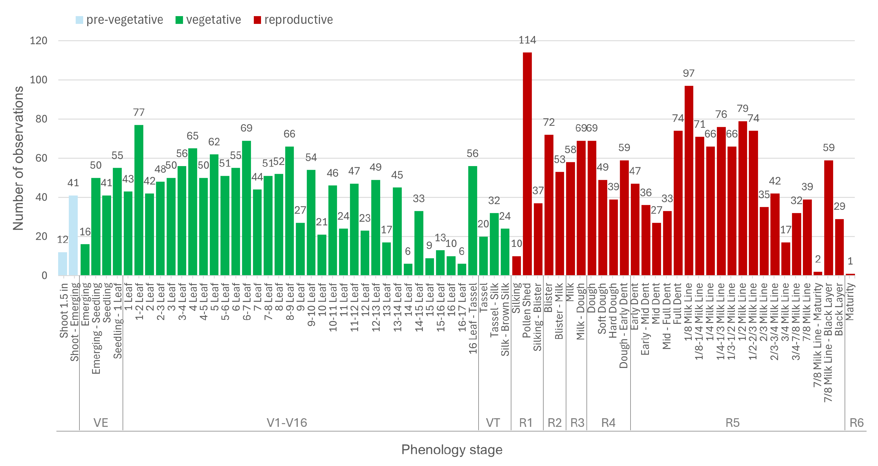
The average field area was 0.5 km2, the smallest field was 0.004 km2 and the largest was 23 km2. Each field underwent approximately five visits during the season, with the frequency varying across all fields; the minimum number of visits was 1 and the maximum was 33. It includes geolocated fields from both regions (south-west and south-central Kansas), crop phenology measurements for each field (observed micro-stages) and the respective date of data collection. Phenology stages followed the scale described in Figure 2, based on [38].
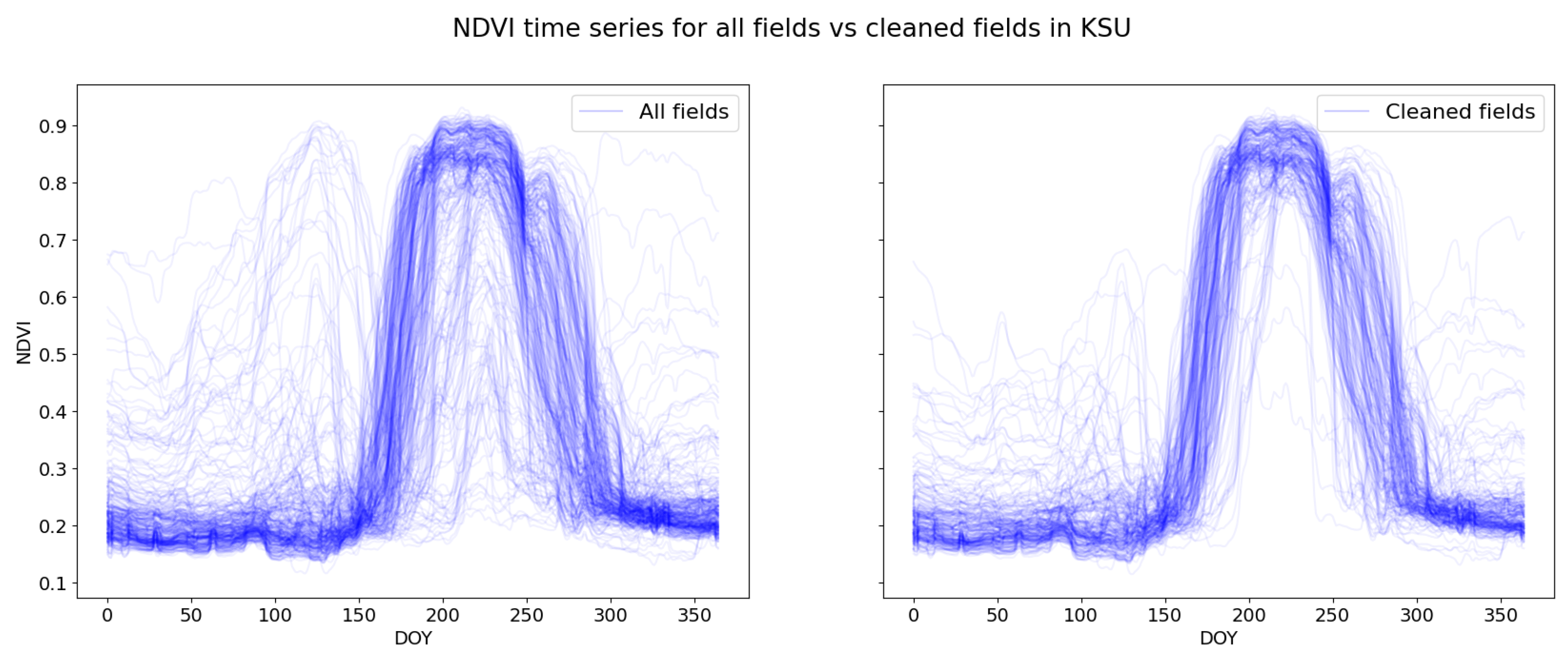
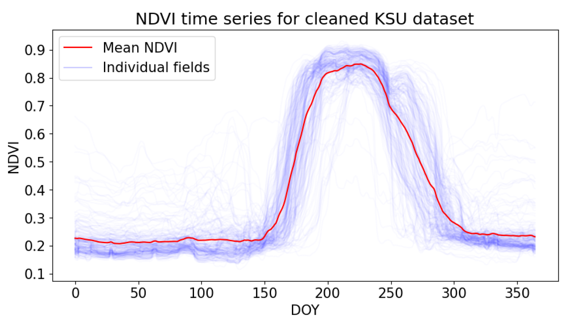
We applied a two-step data cleaning process to the provided field boundaries in order to reduce the potential problems which could negatively impact template creation. In the first step, we calculated the NDVI times series of the fields to apply a clustering using K-Means DTW distance metric, with nine centres. After that, we manually checked and removed clusters of outliers such as those induced by, e.g., wrong crop labels, erroneous field boundaries or partial image coverage. Higher NDVI values before and after the main crop are most likely other crops growing before or after the main crop (cover crops or herbs regrowing after harvest). As a result, from the initial 270 fields, we retained 208 fields for further analysis (Figure 3).
In the second step, we further analyzed the phenology stage observations recorded for these fields, and found that in some cases, stages do not follow chronological order. For example, 3-leaf stages are recorded after 5-leaf stages. We assume the reasons are incorrect manual labeling, intra-field variability, and variation in the points at which the observations were recorded during the season. We aimed to reduce these types of problems by initially identifying misordered observations through a script and subsequently performing manual verification prior to their removal. After the cleaning steps, we had 3714 observations from 208 fields. The number of unique fields for each micro-stage is given in Figure 4. In our study, we excluded harvest and all stages before Emerging (VE). The latter are not expected to be detectable by optical imagery, since they develop underground, while harvested fields were beyond the scope of this study. To draw meaningful conclusions, we opted to focus on micro-stages with substantial data presence; specifically, those with more than five recorded observations. This further reduced the dataset to 3235 observations.
Table 1 provides the traceability between micro-stages and their corresponding macro-stages [39]. Our aim was to detect the micro-stages illustrated in Figure 4. Additionally, as we were comparing the performance of our algorithm on the PIAF dataset explained in the next section, we provide the matched BBCH codes for these macro-stages.

2.2.2. PIAF Dataset

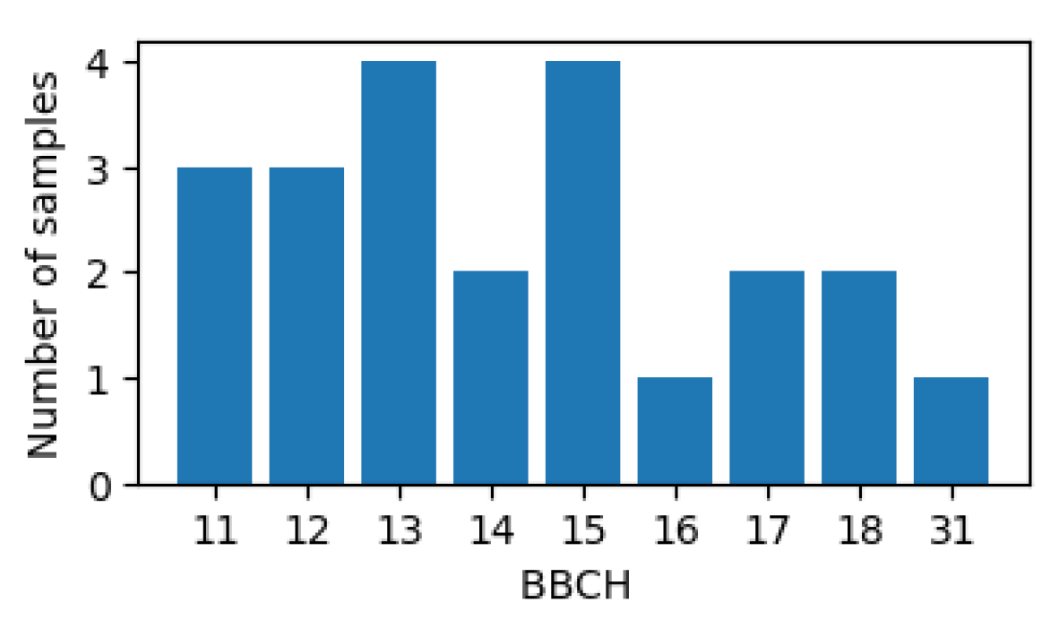
PIAF is the standard program for official plant protection products and variety trials in Germany [40]. It recorded BBCH phenological stage information at coordinate locations for the period 2018–2021. These sites were visited at variable frequencies and durations, but most typically early in the season. The BBCH stage for the location was recorded as a minimum, maximum, and average value; only the average values were used for analysis. Observations of growth stages which were not in the expected chronological order were removed. A subset of these data totaling seven maize fields was made available to us by the Julius Kühn Institute, Germany, in the frame of the NaLamKI project. Field boundary geometries for these fields were sourced from publicly available user-submitted datasets that form the basis of official EU reporting (Integrated Administration and Control System). Figure 5 shows the histogram of BBCH codes for 22 observations, which can be mapped to macro-stages available in the KSU dataset [39].

3. Methodology

3.1. Preparation of the Time Series

Unlike most of the literature studies, we aimed to understand the potential of different spectral features selected or computed from the imagery for the phenology detection problem. Therefore, this paper focused on the individual spectral bands (green, red, and NIR) that are most sensitive to vegetation dynamics, along with the most commonly used spectral indices including Normalized Difference Vegetation Index (NDVI), Enhanced Vegetation Index (EVI), 2-band enhanced vegetation index (EVI2), Kernel Normalized Difference Vegetation Index (kNDVI), Modified Chlorophyll Absorption Ratio Index (MCARI), Chlorophyll Vegetation Index (CVI) and Normalized Difference Water Index (NDWI). These indices were chosen for their proven effectiveness in assessing various aspects of vegetation, such as chlorophyll content, photosynthetic activity, structural attributes and water content, providing comprehensive insights into the physiological status of the vegetation.
The formulas of the selected indices are given in Table 2.

3.2. Dynamic Time Warping with Weighted Average

In this study, we aimed to develop an algorithm to detect the micro-stages given in Table 1. For a target field, t to detect each micro-stage, the algorithm finds the available observations and related fields in the training dataset. The time series of these fields are used as our templates,  S = { s 1 , s 2 , , s n } . To achieve our goal, we leverage DTW for crop phenology detection. DTW is a method used to measure the similarity between two time series denoted as t and  s i , which may fluctuate in time or intensity, such as the NDVI values. Our DTW approach employs the Mori step pattern [47] for managing intricate time relationships, aiding in capturing subtle changes in phenological transitions. Additionally, the Itakura parallelogram [48] windowing function enables the handling of time warping in signals exhibiting non-linear temporal distortions.
The process commences with the construction of a cost matrix, which encapsulates the pairwise distances between all points in t and  s i . Incorporating the specified windowing function confines possible alignments. The Mori step pattern dictates permissible movements during alignment, thus influencing the alignment path within the cost matrix. Subsequently, we calculate the alignment distance,  D t s i , representing the overall dissimilarity between t and  s i  after accounting for temporal variations and intensity disparities.
Following the computation of the cost matrix, the subsequent step entails determining the optimal alignment path. This is accomplished through backtracking, wherein the path with the minimum accumulated cost is traced from the bottom-right corner of the matrix to its top-left corner. Along this path, matched days of year (DOY) between t and  s i  are identified. It is assumed that the function  M i ( )  returns the matched DOY on t for a selected point on  s i . Thus, for an observation,  O s i p , which belongs to the selected micro-stage, p, we can identify the matched DOY in the target field as  M i ( O s i p ) .
After measuring the distances and matching the points for each template in S, the algorithm calculates the confidence score  C t s i  for each template as follows:
C t s i = 1 D t s i max ( D t s )
Then, it calculates weights for each prediction based on these normalized confidence scores, reflecting their relative importance:
W t s i = C t s i k = 1 n C t s k
Thus, for each micro-stage, the algorithm uses the available fields in the training set which have an observation for the selected stage.
y p = W t s i · M i ( O s i p )
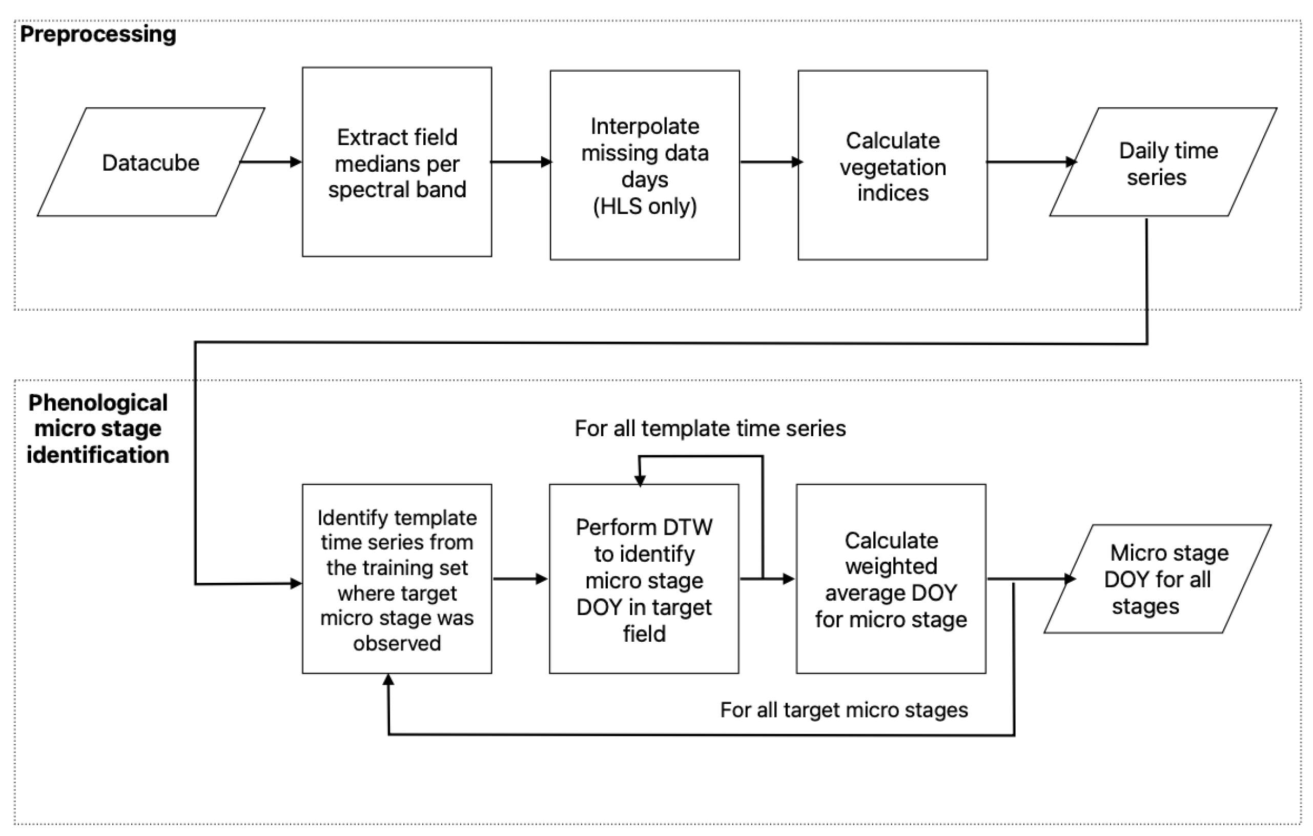
The overall workflow of the proposed method is summarized in Figure 6.

4. Experiments

The algorithm was developed and tested on the Kansas dataset. For the evaluation of the method on unseen maize fields in other regions, we used the PIAF dataset. This was the only dataset available for another geographical region and years with the limitation that the number of maize fields was very small.
Given the restricted number of observations for each phenological stage, we implemented leave-one-out cross-validation for all experiments with the Kansas dataset. This involved systematically excluding the target observation along with related observations from the same field to construct the training set. Templates for DTW matching were then derived from the remaining observations in the training set. DTW was subsequently applied to align the target field with each template, facilitating the detection of micro-stages. This rigorous approach ensured a comprehensive assessment of our method’s capability to accurately identify phenological shifts within the target field.

4.1. Performance Metrics

In order to measure the proposed model, we computed the three statistical measures mean absolute error (MAE), median absolute error (MedAE) and root mean square error (RMSE) for each micro-stage:
MAE = 1 n i = 1 n | y p y p | ,
MedAE = median ( | y p y p | )
and
RMSE = 1 n i = 1 n ( y p y p ) 2 ,
where n is the number of samples,  y p  is the prediction and  y p  is the ground truth (as DOY).
As mentioned above, each field underwent approximately five visits during the season. Therefore, a reported observation does not necessarily signify the beginning of that stage. Most likely, the crop in the field was at the stage on the preceding and succeeding days. It is also important to consider that the same micro-stage could develop at different rates within a few days, depending on specific growing conditions and the particular growth stage of the crop. Hence, achieving a 0-day error is not a practical expectation, and predictions with differences of around one to five days are plausibly accurate.

4.2. Comparison of DTW Methods

To assess the efficacy of our proposed weighted average approach, we conducted a comparative study with two alternative methods using DTW on the PF-NDVI time series.
Method 1—Average Time Series: In this method, we computed the average time series of the training fields and employed it as a reference during the DTW matching process. This approach aimed to provide a baseline since it was used in several studies [28,49] (Figure 7).
Method 2—Single Similar Field: Unlike the conventional approach of utilizing all fields for comparison, we experimented with selecting the most similar field from the training dataset based on the distance metric mentioned earlier. Subsequently, DTW matching was performed exclusively using this selected field:
y p = M j ( O s j p ) , where j = arg max i ( W t s i ) .
Method 3—Weighted Average (Proposed Method): As described in the Methodology section, we proposed a method that applies DTW between the target field and each individual field in the training dataset. After this, we used a weighted averaging approach to calculate the DOY of the selected micro-stage. The weights were determined based on the confidence scores obtained from the distance values.
For each method, we evaluated its performance in detecting micro-stages using PF-NDVI time series (median per field). Comparative analysis was conducted to discern the strengths and limitations of the weighted average approach in contrast to the simpler alternatives. Figure 8 shows the averages of the mean and median absolute errors for the 70 micro-stages. Mean and median absolute errors are smaller for our proposed method.
In addition to the overall performance metrics calculated earlier, our goal was to determine the error for each observation and tally the number of observations detected with errors of up to 1, 5, 10 and 15 days. It is crucial to note that field observers did not visit the fields daily. However, lacking this information, we opted to compute the difference between our predicted and observed days as the error (see Table 3).
Our proposed method successfully identified 90% of the observations within a 10-day error margin. In contrast, method 1 only managed to recognize 79% of the observations within the same error range. Upon examining the bottom 3% of observations, where the error exceeded 15 days, we noted that a significant amount of these observations (49 out of 97) were associated with micro-stages of R5. This higher error rate during the R5 stage can likely be attributed to the subtle physiological changes that occur as the kernels transition from Early Dent to Black Layer, which are not easily distinguishable using remote sensing data. The other 48 were associated with the VE (emergence to seedling) and R4 (dough micro-stages). The same changes during VE and R4 are most likely too subtle to be picked up by the optical signal.

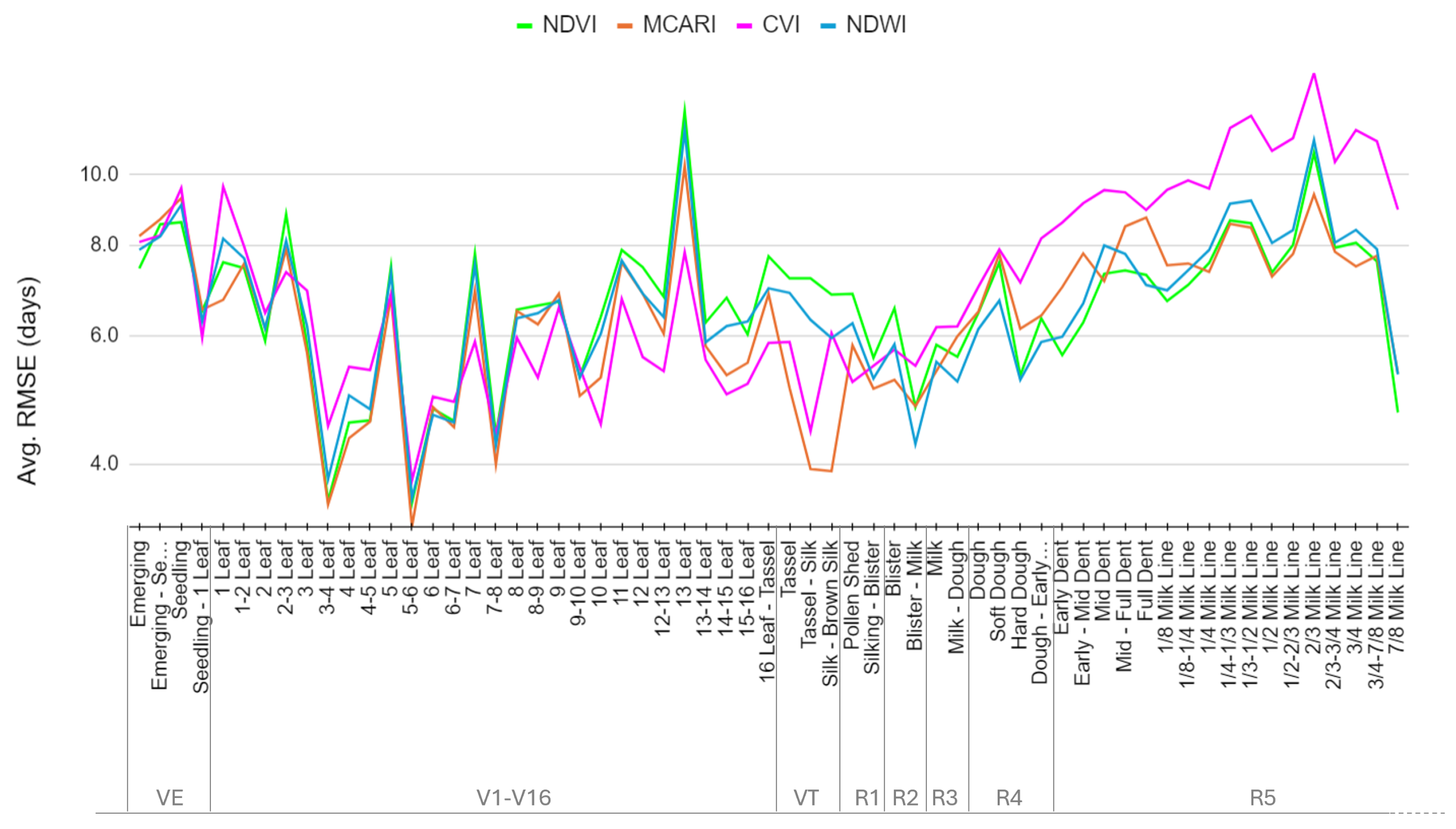
4.3. Performance of Spectral Indices and Bands

In the second experiment, our focus shifted to the input data. We computed various spectral indices derived from PF and used the bands most sensitive to vegetation dynamics (green, red and NIR), as explained in Section 3.1, as input to our proposed DTW method (method 3). For each input type, we conducted experiments separately and evaluated their performance across different phenological stages. Figure 9 shows the performance for NDVI, MCARI, CVI and NDWI indices over all micro-stages. Comparative analysis was conducted to assess the effectiveness of each input type in accurately detecting phenological micro-stages within the target field (RSME values for the selected micro-stages are given in Appendix A Table A1 and Table A3, while the MedAE values are given in Appendix A Table A2 and Table A4).
No single vegetation index outperformed the others across all micro-stages. However, we observed that NDVI and MCARI are the most reliable input types for these 70 micro-stages. For both of them, the average median errors for all stages was around 4 days. For 58 micro-stages, the median error difference was less than 1 day for these two indices. Table 4 shows the performance of the proposed method based on NDVI and MCARI indices for a subset of micro-stages. We observed that MCARI provides better results for the R1 and VT stages. Although CVI has the smallest error from V10 to V16, the RMSE through the reproductive stages and early in the season (V1–V9) is higher than NDVI and MCARI. NDWI always has higher RMSE than at least one other index, except in the Blister—Milk micro-stage. DTW applied to individual spectral bands did not show better performances overall than when applied to spectral indices, and so the spectral bands were discarded from any further analysis. For single-variable methods like DTW, spectral indices seem to be better suited as they combine two or more wavelengths (bands) to enhance the information content of the underlying dataset.

4.4. Comparison of Planet Fusion and HLS

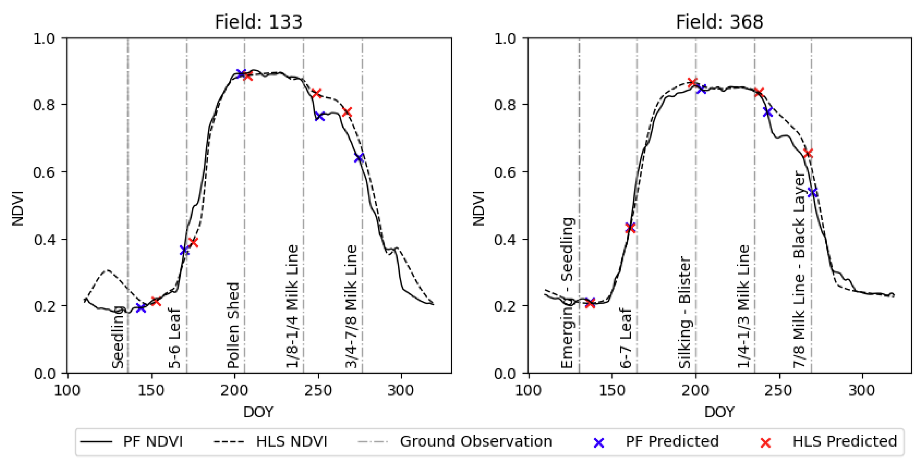
We compared PF to publicly available HLS. For each data source, we evaluated the DTW performance using NDVI and MCARI, as detailed in the preceding section. Figure 10 illustrates the differences in the HLS and PF NDVI time series and detected micro-stages for two example fields. We compared the RMSE performance of the best PF-based DTW solution with that of the best HLS-based DTW solution for each micro-stage. For PF, MCARI performs the best overall, while for HLS, NDVI performs the best overall. PF’s average RMSE values are 2.5 days lower than HLS’s average RMSE values over all 70 micro-stages (RSME values for the selected micro-stages are given in Appendix A Table A5 and Table A6). We observed the biggest differences for V2, R1 and early R5.
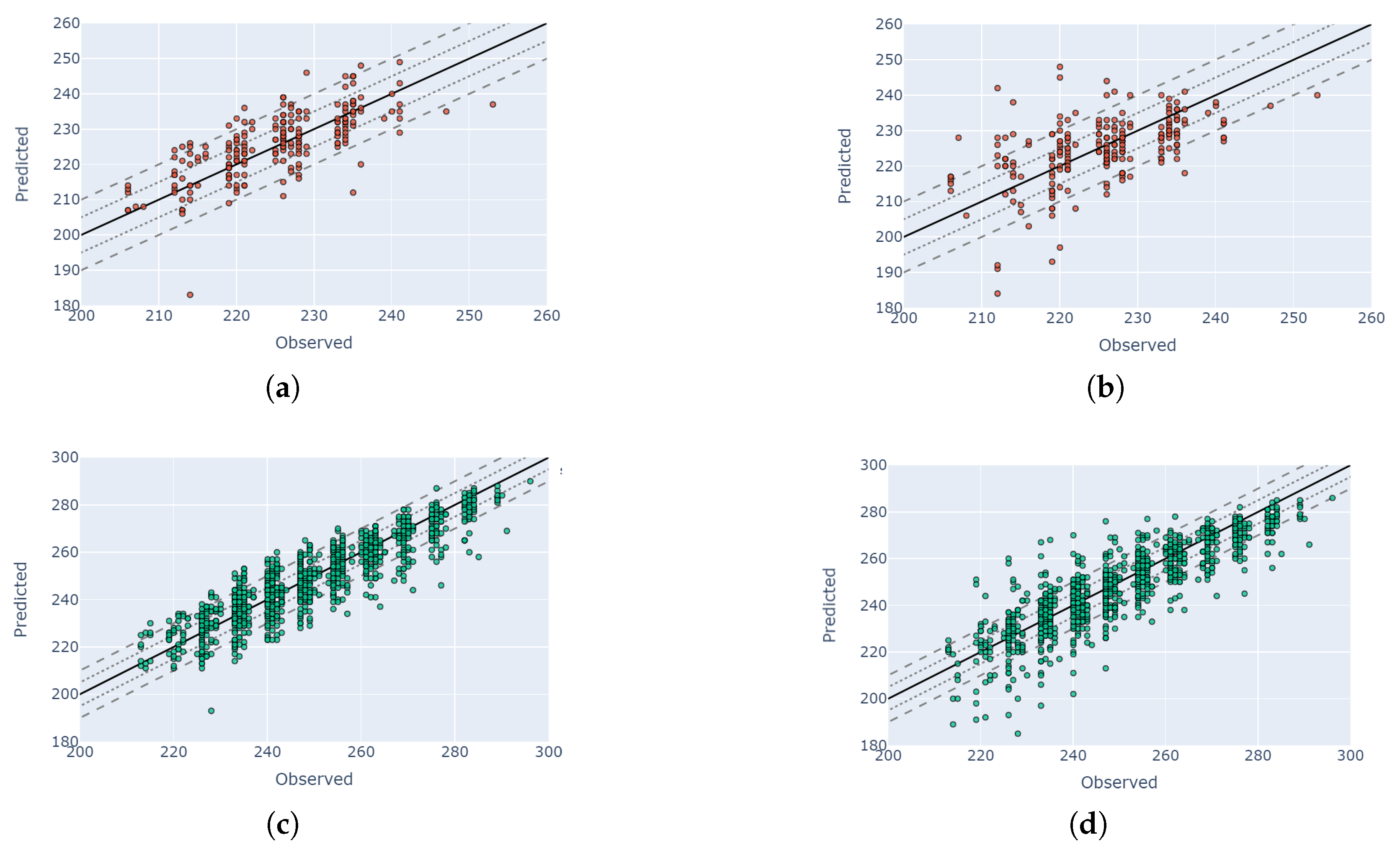
Figure 11 illustrates the comparison between the best PF and HLS DTW solutions for two example macro-stages V4 and R1. During V4–V6 is when nitrogen fertilizer is applied during the growing season (in small doses and in addition to pre-planting) with V6 marking the beginning of rapid growth and uptakes of larger amounts of water and nutrients [50]. Growing conditions around flowering (R1 silking) are important for determining yield, and water stress or shading in this phase negatively affects yield [51]. The orange color represents the observed and predicted days for each observation in the V4 stage, which includes the 4-leaf and 4–5 leaf micro-stages. The pink color indicates the observed and predicted days for each observation in the R1 flowering stage (Figure 11b). When we count the number of micro-stages where at least 80% of the samples were detected within a five-day error margin, HLS achieved this accuracy only for the 5–6-leaf stage, with a rate of 80.4%. In contrast, the PF-based method detected at least 80% of the samples within a five-day error margin for all micro-stages from ‘3–4-leaf’ to ‘7–8-leaf’, with the highest sample ratio being 86% for the ‘5–6-leaf’ stage. HLS had its worst performance at the ‘seedling’ stage, where only 59% of the samples were detected within a 10-day error margin. The PF method’s lowest ratio was 67%, observed at the ‘16–17-leaf’ stage within a 10-day error margin.
We observed similar patterns for the rest of the phenological stages. Figure 12 shows a one-to-one comparison for macro-stages V8, R4 and R5. For both data sources (PF and HLS), we picked the index with the best performance, as mentioned above. As mentioned in Section 4.2, the R5 macro-stage has a higher error margin compared to other stages.

4.5. Visual Validation for PIAF Fields

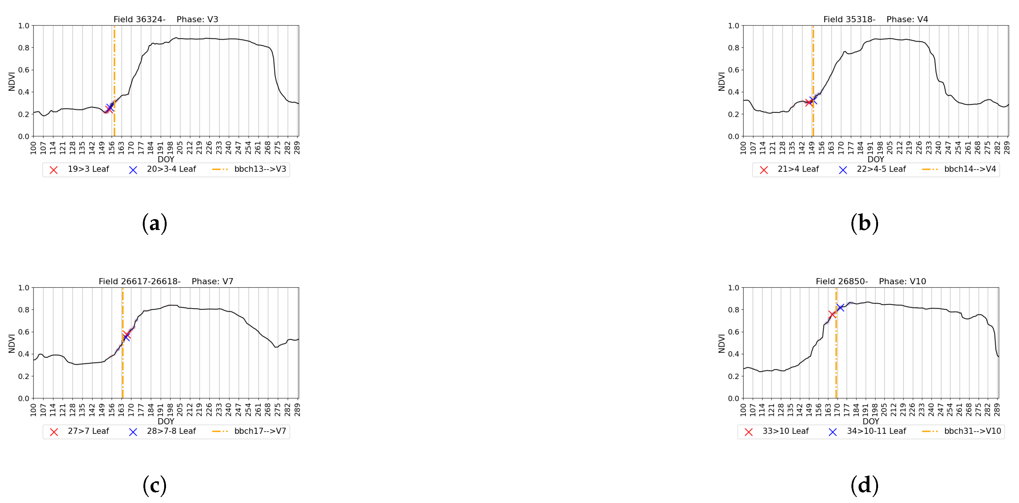
It is essential to assess the robustness of the proposed model against temporal and spatial variability. To accomplish this, we utilized the PIAF dataset, as outlined in Section 2.2.2. All fields were located in Germany, with observation years being either 2018 or 2019. We used all Kansas fields as templates and applied our model to these seven fields. Due to the limited number of fields and observations (22 observations), we could only visually validate the model and conclude only on the overall performance. Additionally, the phenology dataset employed different categorizations of phenology stages following the BBCH scale. Therefore, our aim was to detect macro-stages corresponding to BBCH stages (as shown in Table 1). Figure 13 displays the BBCH stage of an observation and the detection results of the corresponding US-scale macro-stages for four different fields. If the observed macro-stage falls within the detected micro-stages (e.g., Figure 13d), we consider the macro-stage prediction correct. Otherwise, we calculate the distance between the observation and the nearest prediction of the related micro-stages. In total, 9 out of the 22 observations (41%) were error-free. The average error for all observations was 3.6 days. Similar to our KSU dataset results, most predictions were within a 10-day buffer compared to the ground truth.

5. Discussion and Conclusions

In this study, we proposed a novel method for maize phenology detection using Dynamic Time Warping (DTW) applied to daily time series of optical imagery. We compared the novel analysis-ready PF data and HLS data, limiting the analysis to the spectral bands both datasets had in common (R, G, B, NIR). Both were processed using daily datasets to evaluate the possibility of capturing subtle changes in crop development. We evaluated the model’s performance across 70 micro-stages, leveraging a dataset comprising more than 200 fields and 3235 observations. Our DTW strategy aligns target fields with templates, calculates distances between time series and derives confidence scores for predictions. Unlike methods relying on a singular template [28], our approach preserves crucial patterns in the data. We highlight the significance of individual observations in prediction accuracy and reduce the impact of potential labeling issues. In addition to examining individual bands, we investigated eight commonly employed indices as inputs. Our observations revealed that NDVI and MCARI indices show particular promise. Across all stages, for PF, the average median errors for both indices were approximately 4 days. Notably, we found that MCARI yields comparatively superior results, especially for the VT and R1 stages, at the transition between vegetative and reproductive stages and during the peak of biomass. This could be due to NDVI and MCARI more closely representing the physical characteristics of each maize growth stage. Both VI have been shown to have a strong correlation with maize canopy cover changes [52] and NDVI has been shown to strongly relate to biomass accumulation in the V1–V10 macro-stages [53]. Although the EVI and EVI2 also measure these features, NDVI has been shown to better characterize the start-of-season growth for maize [54]. In the reproductive growth stages, MCARI has been demonstrated to have a stronger relationship with chlorophyll content than NDVI and CVI [55], possibly due to the saturation of NDVI at high biomass levels and CVI being largely driven by greenness. CVI also performed better in the V10–V16 stages due to greenness and saturation of NDVI. For HLS, NDVI performed better overall.
Additionally, for the best result with PF-MCARI, we observed that the difference between observation and prediction was equal to or less than 5 days for 2025 of the observations (65%), and 2900 (90%) of the observations had a maximum distance of 10 days. For all micro-stages from ‘3-4-leaf’ to ‘7-8-leaf’, at least 80% of the samples were detected within a five-day error margin, with the highest accuracy reaching 86%. Only 3% of the overall observations had a difference of more than 15 days, with more than half of these observations belonging to the micro-stages of R5, the last macro-stage before maturity. This macro-stage contains the highest number of micro-stages. The performance of the proposed method is particularly promising, considering that field observers did not visit the fields daily. Consequently, reported observations may not accurately represent the exact initiation of each stage. Furthermore, it is impractical and logistically challenging to compile a dataset where phenological stages are recorded daily throughout the growing season across multiple fields. Such an undertaking would require substantial labor and resources, which are often not feasible. Additionally, many micro-stages are nearly imperceptible to the naked eye, complicating accurate field observations. Therefore, expecting zero-day error is unrealistic. Given these constraints, the fact that 97% of the provided predictions fall within acceptable limits underscores the robustness and reliability of the proposed method.
To understand the advantages of Planet Fusion (PF), a daily gap-free, cloud-free, harmonized analysis-ready image dataset, we compared it with the publicly available HLS dataset. PF outperforms HLS, with significant improvements observed in key phenological stages like V4, R1 and late R5. PF is analysis-ready data supplied at a daily resolution, whereas HLS needed to undergo interpolation to produce a daily time series. The selected interpolation approach has an impact on the time series characteristics. As different interpolation approaches were not compared as part of this study, it is possible that the performance of HLS could be improved with a different interpolation algorithm or a more complex gap-filling approach using previous years and proximate pixel values, like PF processing. However, it seems probable that the largest impact on performance is attributable to the difference in raw image volume. Across the year 2017 in the Kansas dataset, for each field, an average of 110.99 PlanetScope observations formed the basis of PF for gap-filling. On the other hand, an average of 44.25 HLS observations were interpolated into a daily time series. Note that the eastern Kansas site had many cloud days and lower data frequency. The average number of days between observations was 8.33 for HLS and 3.25 for PF. As there are more images in PF, it is more likely to have captured changes in spectral reflectance that might indicate changes in the phenological stage. This is exacerbated by the HLS data for 2017 including only one of the Sentinel-2 satellites until July 6th. The increased cadence of PlanetScope data as a source constellation and the gap-filling approach of PF, which also uses signals from other sensors such as Sentinel-2, may be the reason that phenology micro-stages can be better identified in PF.
Finally, we aimed to demonstrate the model’s transferability to different regions and years. We used the Kansas dataset observations to detect stages in seven fields in Germany during 2019 and 2020. The average error was 3.6 days for the 22 observations. The results show its potential applicability across diverse regions and years. However, to provide statistically proven results, it is crucial to increase the number of fields from Germany or obtain additional data from any other region. Unfortunately, phenology observation datasets at this level of detail are very difficult to access. These detailed datasets are not available for all regions globally, limiting the applicability of this approach outside of North America and Europe. Our study hints at what could be achieved when such detailed phenology datasets are combined with the latest technology in remote sensing and machine learning. Further data are needed to validate these approaches for regional-scale research. Remote sensing data could improve crop growth models which are currently based on weather data only (e.g., [56,57]) and show variability in predictive power throughout the season. While our study demonstrates the robustness and efficiency of the DTW algorithm in detecting maize phenology stages, we did not focus on optimizing the computational aspects of the code. For application in very large regions, further optimization may be necessary. Additionally, the DTW method can be used in a knowledge distillation framework, where it serves as a teacher model to train a deep learning-based solution, thereby enhancing scalability and performance.
As a direction for future research, we aim to expand the scope of our study by redefining the problem. Instead of identifying a single day of year (DOY) for each micro-stage, we intend to approach it as a segmentation problem, where the model predicts both the start and end dates of each micro-stage. This adjustment will provide a more comprehensive understanding of the phenological dynamics. Furthermore, we intend to explore the variations in plant growth within individual fields. Rather than relying on a single median or mean value for a given day, we aim to leverage the entire field’s pixel data to capture phenology variability within each field accurately. Lastly, we will explore in-season phenology detection for fields where it is known that the planted crop is maize. Our current methodology focuses on retrospectively analyzing the entire time series to determine the timing of each stage; although understanding historical crop phenology is crucial for understanding long-term trends in agricultural productivity and management, there is a growing need in various application domains to ascertain the current phenological stage for timely decision-making. By addressing these aspects, we aim to enhance the robustness and applicability of our model across diverse agricultural landscapes and temporal contexts.

Author Contributions

Conceptualization, C.S., A.W., A.S.R., M.G. and P.H.; methodology, C.S.; software, C.S.; validation, C.S. and A.S.R.; formal analysis, C.S.; investigation, C.S.; data curation, M.G. and A.S.R.; writing—original draft preparation, C.S., M.G. and A.W.; writing—review and editing, L.N., P.H., I.C., A.S.R. and T.D.; visualization, C.S., M.G., L.N. and A.S.R.; supervision, C.S. and A.W.; project administration, A.W. All authors have read and agreed to the published version of the manuscript.

Funding

The work was performed under the research project NaLamKI, which received funding from the Federal Ministry for Economic Affairs and Climate Action of Germany BMWK (Teilvorhaben 01MK21003G).

Data Availability Statement

Restrictions apply to the availability of these datasets. Kansas data were obtained from K-State University and are available from the authors with the permission of CropQuest. Access to PIAF data was enabled by the Julius Kühn Institute, Germany, in the frame of the NaLamKI project.

Acknowledgments

We are grateful to Tanja Riedel from the Julius Kühn Institute, Germany (JKI), for preparing the PIAF data and discussing the experiments. Furthermore, we thank Rasmus Houborg (Planet Labs PBC) for processing Fusion data and for his inputs to the design of experiments. The findings and views described herein do not necessarily reflect those of Planet Labs PBC.

Conflicts of Interest

Authors C.S., A.W., A.S.R., M.G., T.D. and P.H. are employed by Planet Labs. The remaining authors declare that the research was conducted in the absence of any commercial or financial relationships that could be construed as a potential conflict of interest.

Appendix A

Table A1. RMSE in days for the selected vegetative micro-stages calculated for the selected indices and bands using Planet Fusion (best values are in bold).
Stage    NDVIMCARIEVIEVI2CVIkNDVINDWIBand GBand RBand NIR
VE: Emerging7.48.28.17.48.17.37.98.67.710.8
VE: Emerging—Seedling8.58.77.38.58.38.68.25.95.98.2
VE: Seedling8.69.37.98.59.68.49.18.07.98.5
VE: Seedling—1-leaf6.56.55.86.56.06.66.36.66.48.7
V1: 1-leaf7.66.76.87.59.67.58.28.27.712.2
V1: 1–2-leaf7.47.67.17.58.07.57.76.56.69.9
V2: 2-leaf5.96.25.55.96.56.06.15.45.08.4
V2: 2–3-leaf8.87.98.98.87.38.88.19.29.79.3
V3: 3-leaf5.85.75.65.86.95.96.26.36.17.8
V3: 3–4-leaf3.63.53.43.54.53.63.84.34.27.6
V4: 4-leaf4.64.34.24.65.44.65.04.94.57.8
V4: 4–5-leaf4.64.64.64.65.44.64.85.95.57.4
V5: 5-leaf7.56.87.77.56.97.57.38.08.38.4
V5: 5–6-leaf3.53.33.33.53.83.53.64.04.07.9
V6: 6-leaf4.84.84.94.85.04.84.75.25.17.6
V6: 6–7-leaf4.64.54.64.54.94.54.65.14.96.0
V7: 7-leaf7.86.98.17.85.97.97.58.68.77.6
V7: 7–8-leaf4.44.04.54.24.44.34.24.84.75.0
V8: 8-leaf6.56.56.66.56.06.56.36.56.67.8
V8: 8–9-leaf6.66.27.06.65.36.66.57.17.36.8
V9: 9-leaf6.76.96.96.86.66.86.76.86.86.8
V9: 9–10-leaf5.35.05.45.25.45.15.35.75.65.1
V10: 10-leaf6.45.36.56.34.56.46.05.66.24.7
V11: 10–11-leaf7.96.78.47.85.77.87.38.58.76.2
V11: 11-leaf7.97.68.37.86.77.97.67.27.78.9
V12: 11–12-leaf6.96.36.96.95.96.86.76.66.95.3
V12: 12-leaf7.56.97.97.45.67.56.96.77.26.5
V12: 12–13-leaf6.86.06.96.85.46.86.46.46.75.8
V13: 13-leaf12.210.313.412.17.812.411.512.713.57.0
V13: 13–14-leaf6.35.86.26.25.66.25.96.46.45.3
V14: 14–15-leaf6.85.37.26.85.06.86.26.46.45.3
V15: 15–16-leaf6.05.56.16.05.26.26.35.55.75.4
V16: 16-leaf—Tassel7.76.98.87.75.97.67.08.59.26.3
VT: Tassel7.25.16.97.25.97.16.97.16.66.0
VT: Tassel—Silk7.23.97.17.24.47.26.36.06.94.3
VT: Silk—Brown Silk6.83.96.96.86.16.76.07.68.16.1
Table A2. MedAE in days for the selected vegetative micro-stages calculated for the selected indices and bands using Planet Fusion (best values are in bold).
Stage    NDVIMCARIEVIEVI2CVIkNDVINDWIBand GBand RBand NIR
VE: Emerging4.06.05.54.05.54.05.06.55.07.5
VE: Emerging—Seedling5.04.05.05.56.06.05.54.04.54.0
VE: Seedling6.06.06.06.08.06.07.06.05.04.0
VE: Seedling—1-leaf4.05.04.04.04.04.05.05.05.07.0
V1: 1-leaf6.04.05.06.05.06.05.03.04.05.0
V1: 1–2-leaf5.04.04.05.05.05.05.03.04.06.0
V2: 2-leaf3.53.03.03.53.53.53.53.02.55.0
V2: 2–3-leaf3.03.02.03.02.02.53.03.03.05.0
V3: 3-leaf3.53.03.03.04.03.54.03.53.05.0
V3: 3–4-leaf2.02.02.02.02.52.02.53.02.03.0
V4: 4-leaf3.03.03.03.04.03.04.03.03.04.0
V4: 4–5-leaf3.02.53.03.03.03.03.03.03.05.0
V5: 5-leaf3.02.03.03.03.53.03.03.03.05.0
V5: 5–6-leaf3.02.02.03.03.03.02.03.03.04.0
V6: 6-leaf2.02.02.02.03.02.02.02.02.04.0
V6: 6–7-leaf3.02.03.03.03.03.03.03.03.04.0
V7: 7-leaf3.03.03.03.03.53.03.02.02.04.0
V7: 7–8-leaf3.02.03.03.03.03.02.03.03.03.0
V8: 8-leaf4.04.04.04.03.54.04.04.04.03.0
V8: 8–9-leaf3.03.53.03.03.53.03.03.03.03.5
V9: 9-leaf3.03.02.03.04.03.03.03.03.04.0
V9: 9–10-leaf4.03.04.04.03.54.04.04.04.03.0
V10: 10-leaf3.03.04.03.03.03.03.04.04.04.0
V11: 11-leaf5.56.05.55.54.05.55.04.05.06.0
V12: 12-leaf5.04.05.05.05.05.04.05.05.05.0
V12: 12–13-leaf5.04.05.05.04.05.05.05.05.04.0
V13: 13-leaf6.06.05.05.06.05.06.06.06.05.0
V13: 13–14-leaf5.05.05.05.04.05.05.06.06.04.0
V14: 14–15-leaf4.03.05.04.03.04.04.05.04.03.0
V15: 15–16-leaf5.06.04.05.03.05.04.03.04.03.0
V16: 16-leaf—Tassel5.55.05.05.04.05.05.05.06.05.0
VT: Tassel6.04.05.56.04.56.06.05.55.05.0
VT: Tassel—Silk5.03.04.55.03.05.05.05.06.03.0
VT: Silk—Brown Silk5.53.05.05.55.05.54.08.08.02.5
Table A3. RMSE in days for the selected reproductive micro-stages calculated for indices and bands using Planet Fusion (best values are in bold).
Stage     PF NDVIPF MCARIEVIEVI2CVIkNDVINDWIBand GBand RBand NIR
R1: Pollen Shed6.95.87.46.85.26.96.27.37.76.1
R1: Silking—Blister5.65.16.25.65.55.65.26.15.65.9
R2: Blister6.65.27.16.55.76.55.86.66.87.2
R2: Blister—Milk4.84.85.64.75.54.84.34.24.66.0
R3: Milk5.85.46.55.86.25.75.56.86.37.3
R3: Milk—Dough5.66.06.45.66.25.65.25.55.57.5
R4: Dough6.56.57.86.57.06.56.16.16.17.7
R4: Soft Dough7.67.810.27.67.97.66.78.99.18.6
R4: Hard Dough5.36.16.55.47.15.35.26.56.37.0
R4: Dough—Early Dent6.36.47.46.38.26.45.96.46.28.3
R5: Early Dent5.67.07.25.68.65.66.05.96.08.6
R5: Early—Mid Dent6.37.88.06.39.16.36.76.76.79.1
R5: Mid Dent7.37.16.77.49.57.28.07.46.67.4
R5: Mid—Full Dent7.48.57.37.39.57.47.87.16.210.6
R5: Full Dent7.38.79.37.28.97.37.17.26.99.6
R5: 1/8 Milk Line6.77.57.86.79.56.76.97.57.18.8
R5: 1/8–1/4 Milk Line7.17.68.27.09.87.17.48.37.59.3
R5: 1/4 Milk Line7.67.48.27.59.67.57.97.97.58.0
R5: 1/4–1/3 Milk Line8.78.68.98.611.68.69.110.08.710.1
R5: 1/3–1/2 Milk Line8.68.59.18.612.18.59.28.58.68.6
R5: 1/2 Milk Line7.37.27.47.310.87.38.18.47.78.1
R5: 1/2–2/3 Milk Line8.07.88.27.911.28.08.48.08.29.2
R5: 2/3 Milk Line10.79.411.010.613.810.611.210.610.810.3
R5: 2/3–3/4 Milk Line7.97.88.47.910.47.88.17.67.99.3
R5: 3/4 Milk Line8.17.57.78.111.58.18.412.09.010.3
R5: 3/4–7/8 Milk Line7.67.78.07.511.17.57.910.28.29.1
R5: 7/8 Milk Line4.75.35.04.79.04.75.38.25.67.1
R5: 7/8 Milk L.—Black L.8.79.38.98.712.18.79.19.28.512.4
R5: Black Layer8.37.88.28.212.08.19.110.87.98.5
Table A4. MedAE in days for the selected reproductive micro-stages calculated for indices and bands using Planet Fusion (best values are in bold).
Stage     PF NDVIPF MCARIEVIEVI2CVIkNDVINDWIBand GBand RBand NIR
R1: Pollen Shed5.03.04.05.04.04.55.05.05.04.0
R1: Silking—Blister5.02.04.05.04.05.04.04.05.04.0
R2: Blister5.04.04.04.53.04.54.04.54.05.0
R2: Blister—Milk3.03.03.03.04.03.03.03.03.04.0
R3: Milk3.04.04.53.04.03.03.04.03.55.0
R3: Milk—Dough4.05.04.04.04.04.04.03.03.05.0
R4: Dough4.04.06.04.04.04.04.03.04.06.0
R4: Soft Dough4.04.06.04.05.04.04.04.05.06.0
R4: Hard Dough3.05.04.03.05.03.03.04.03.05.0
R4: Dough—Early Dent4.06.06.04.05.04.03.03.04.07.0
R5: Early Dent4.06.05.05.06.05.05.04.04.07.0
R5: Early–Mid Dent4.56.05.04.56.54.55.04.05.07.0
R5: Mid Dent5.04.05.05.08.04.06.04.04.06.0
R5: Mid–Full Dent4.06.06.04.06.04.04.04.04.07.0
R5: Full Dent5.06.06.05.07.55.06.05.06.07.0
R5: 1/8 Milk Line5.05.07.05.06.05.04.04.05.06.0
R5: 1/8–1/4 Milk Line4.05.06.04.06.04.04.06.05.06.0
R5: 1/4 Milk Line4.05.05.04.05.04.04.05.05.05.0
R5: 1/4–1/3 Milk Line6.06.56.06.07.06.06.06.57.07.0
R5: 1/3–1/2 Milk Line5.05.05.55.06.05.05.06.05.06.0
R5: 1/2 Milk Line5.05.05.05.07.05.05.05.05.05.0
R5: 1/2–2/3 Milk Line5.04.05.05.06.05.05.05.06.05.0
R5: 2/3 Milk Line6.04.06.06.05.06.05.06.05.07.0
R5: 2/3–3/4 Milk Line3.04.04.53.06.03.04.04.55.06.0
R5: 3/4 Milk Line4.05.04.04.05.04.05.07.03.06.0
R5: 3/4–7/8 Milk Line4.54.55.04.56.54.55.08.54.08.0
R5: 7/8 Milk Line3.03.04.03.05.03.04.06.03.04.0
R5: 7/8 Milk L.—Black L.5.05.04.05.07.05.05.06.04.07.0
R5: Black Layer6.05.05.06.07.06.07.06.05.07.0
Table A5. Comparison of PF and HLS RMSE performances for the selected vegetative micro-stages. For each micro-stage, the best PF- and HLS-based performance values are given in bold.
StagePF NDVIPF MCARIHLS NDVIHLS MCARI
VE: Emerging7.48.214.09.5
VE: Emerging—Seedling8.58.710.111.6
VE: Seedling8.69.310.813.2
VE: Seedling—1-leaf6.56.511.29.7
V1: 1-leaf7.66.77.511.6
V1: 1–2-leaf7.47.69.29.9
V2: 2-leaf5.96.28.211.7
V2: 2–3-leaf8.87.98.69.5
V3: 3-leaf5.85.79.48.8
V3: 3–4-leaf3.63.57.47.4
V4: 4-leaf4.64.36.910.5
V4: 4–5-leaf4.64.66.26.0
V5: 5-leaf7.56.87.99.9
V5: 5–6-leaf3.53.34.45.7
V6: 6-leaf4.84.85.97.0
V6: 6–7-leaf4.64.56.68.0
V7: 7-leaf7.86.97.37.2
V7: 7–8-leaf4.44.06.15.4
V8: 8-leaf6.56.57.17.3
V8: 8–9-leaf6.66.29.07.9
V9: 9-leaf6.76.96.86.5
V9: 9–10-leaf5.35.08.16.9
V10: 10-leaf6.45.37.114.4
V10: 10–11-leaf7.96.711.09.3
V11: 11-leaf7.97.68.68.3
V11: 11–12-leaf6.96.39.68.8
V12: 12-leaf7.56.97.78.0
V12: 12–13-leaf6.86.09.29.7
V13: 13-leaf12.210.313.213.5
V13: 13–14-leaf6.35.88.97.7
V14: 14–15-leaf6.85.310.28.7
V15: 15–16-leaf6.05.512.311.2
V16: 16-leaf—Tassel7.76.912.110.3
VT: Tassel7.25.110.78.9
VT: Tassel—Silk7.23.99.99.8
VT: Silk—Brown Silk6.83.96.44.5
Table A6. Comparison of PF and HLS RMSE performances for the selected reproductive micro-stages. For each micro-stage, the best PF- and HLS-based performance values are given in bold.
StagePF NDVIPF MCARIHLS NDVIHLS MCARI
R1: Pollen Shed6.95.810.49.4
R1: Silking—Blister5.65.111.47.9
R2: Blister6.65.29.29.1
R2: Blister—Milk4.84.810.47.9
R3: Milk5.85.411.011.2
R3: Milk—Dough5.66.09.19.3
R4: Dough6.56.59.98.2
R4: Soft Dough7.67.810.08.1
R4: Hard Dough5.36.19.711.6
R4: Dough—Early Dent6.36.48.07.8
R5: Early Dent5.67.09.08.1
R5: Early–Mid Dent6.37.87.57.9
R5: Mid Dent7.37.18.712.8
R5: Mid–Full Dent7.48.510.910.3
R5: Full Dent7.38.710.19.7
R5: 1/8 Milk Line6.77.59.78.9
R5: 1/8-1/4 Milk Line7.17.69.39.3
R5: 1/4 Milk Line7.67.410.09.3
R5: 1/4-1/3 Milk Line8.78.69.68.5
R5: 1/3-1/2 Milk Line8.68.510.29.5
R5: 1/2 Milk Line7.37.27.77.6
R5: 1/2-2/3 Milk Line8.07.810.39.5
R5: 2/3 Milk Line10.79.410.610.3
R5: 2/3-3/4 Milk Line7.97.87.910.2
R5: 3/4 Milk Line8.17.57.28.3
R5: 3/4-7/8 Milk Line7.67.710.69.2
R5: 7/8 Milk Line4.75.36.06.7
R5: 7/8 Milk Line—B. Layer8.79.39.110.6
R5: Black Layer8.37.811.47.7
Average (all stages)6.96.59.09.1

References

  1. Zeng, L.; Wardlow, B.D.; Xiang, D.; Hu, S.; Li, D. A review of vegetation phenological metrics extraction using time-series, multispectral satellite data. Remote Sens. Environ. 2020, 237, 111511. [Google Scholar] [CrossRef]
  2. Gao, F.; Zhang, X. Mapping Crop Phenology in Near Real-Time Using Satellite Remote Sensing: Challenges and Opportunities. J. Remote Sens. 2021, 2021, 8379391. [Google Scholar] [CrossRef]
  3. Pipia, L.; Belda, S.; Franch, B.; Verrelst, J. Trends in Satellite Sensors and Image Time Series Processing Methods for Crop Phenology Monitoring. In Information and Communication Technologies for Agriculture—Theme I: Sensors; Springer International Publishing: Cham, Switzerland, 2022; pp. 199–231. [Google Scholar] [CrossRef]
  4. Helman, D. Land surface phenology: What do we really ‘see’ from space? Sci. Total Environ. 2018, 618, 665–673. [Google Scholar] [CrossRef] [PubMed]
  5. Pan, Z.; Huang, J.; Zhou, Q.; Wang, L.; Cheng, Y.; Zhang, H.; Blackburn, G.A.; Yan, J.; Liu, J. Mapping crop phenology using NDVI time-series derived from HJ-1 A/B data. Int. J. Appl. Earth Obs. Geoinf. 2015, 34, 188–197. [Google Scholar] [CrossRef]
  6. Jonas Schreier, G.G.; Dubovyk, O. Crop-specific phenomapping by fusing Landsat and Sentinel data with MODIS time series. Eur. J. Remote Sens. 2021, 54, 47–58. [Google Scholar] [CrossRef]
  7. Lu, L.; Wang, C.; Gao, H.; Li, Q. Detecting winter wheat phenology with SPOT-VEGETATION data in the North China Plain. Geocarto Int. 2014, 29, 244–255. [Google Scholar] [CrossRef]
  8. Rodigheri, G.; Sanches, I.D.; Richetti, J.; Tsukahara, R.Y.; Lawes, R.; Bendini, H.d.N.; Adami, M. Estimating Crop Sowing and Harvesting Dates Using Satellite Vegetation Index: A Comparative Analysis. Remote Sens. 2023, 15, 5366. [Google Scholar] [CrossRef]
  9. Xu, X.; Conrad, C.; Doktor, D. Optimising Phenological Metrics Extraction for Different Crop Types in Germany Using the Moderate Resolution Imaging Spectrometer (MODIS). Remote Sens. 2017, 9, 254. [Google Scholar] [CrossRef]
  10. Yang, Y.; Tao, B.; Liang, L.; Huang, Y.; Matocha, C.; Lee, C.D.; Sama, M.; Masri, B.E.; Ren, W. Detecting Recent Crop Phenology Dynamics in Corn and Soybean Cropping Systems of Kentucky. Remote Sens. 2021, 13, 1615. [Google Scholar] [CrossRef]
  11. d’Andrimont, R.; Taymans, M.; Lemoine, G.; Ceglar, A.; Yordanov, M.; van der Velde, M. Detecting flowering phenology in oil seed rape parcels with Sentinel-1 and -2 time series. Remote Sens. Environ. 2020, 239, 111660. [Google Scholar] [CrossRef]
  12. Harfenmeister, K.; Itzerott, S.; Weltzien, C.; Spengler, D. Detecting Phenological Development of Winter Wheat and Winter Barley Using Time Series of Sentinel-1 and Sentinel-2. Remote Sens. 2021, 13, 5036. [Google Scholar] [CrossRef]
  13. Zhou, M.; Ma, X.; Wang, K.; Cheng, T.; Tian, Y.; Wang, J.; Zhu, Y.; Hu, Y.; Niu, Q.; Gui, L.; et al. Detection of phenology using an improved shape model on time-series vegetation index in wheat. Comput. Electron. Agric. 2020, 173, 105398. [Google Scholar] [CrossRef]
  14. Gao, F.; Anderson, M.; Daughtry, C.; Karnieli, A.; Hively, D.; Kustas, W. A within-season approach for detecting early growth stages in corn and soybean using high temporal and spatial resolution imagery. Remote Sens. Environ. 2020, 242, 111752. [Google Scholar] [CrossRef]
  15. Gao, F.; Anderson, M.C.; Hively, W.D. Detecting Cover Crop End-Of-Season Using VENµS and Sentinel-2 Satellite Imagery. Remote Sens. 2020, 12, 3524. [Google Scholar] [CrossRef]
  16. Zhang, C.; Xie, Z.; Shang, J.; Liu, J.; Dong, T.; Tang, M.; Feng, S.; Cai, H. Detecting winter canola (Brassica napus) phenological stages using an improved shape-model method based on time-series UAV spectral data. Crop J. 2022, 10, 1353–1362. [Google Scholar] [CrossRef]
  17. Chen, S.; Yi, Q.; Wang, F.; Zheng, J.; Li, J. Improving the matching degree between remotely sensed phenological dates and physiological growing stages of soybean by a dynamic offset-adjustment strategy. Sci. Total Environ. 2024, 906, 167783. [Google Scholar] [CrossRef] [PubMed]
  18. Houborg, R.; McCabe, M.F. Daily Retrieval of NDVI and LAI at 3 m Resolution via the Fusion of CubeSat, Landsat, and MODIS Data. Remote Sens. 2018, 10, 890. [Google Scholar] [CrossRef]
  19. Shen, Y.; Zhang, X.; Yang, Z.; Ye, Y.; Wang, J.; Gao, S.; Liu, Y.; Wang, W.; Tran, K.H.; Ju, J. Developing an operational algorithm for near-real-time monitoring of crop progress at field scales by fusing harmonized Landsat and Sentinel-2 time series with geostationary satellite observations. Remote Sens. Environ. 2023, 296, 113729. [Google Scholar] [CrossRef]
  20. Nieto, L.; Houborg, R.; Zajdband, A.; Jumpasut, A.; Prasad, P.V.; Olson, B.J.; Ciampitti, I.A. Impact of high-cadence earth observation in maize crop phenology classification. Remote Sens. 2022, 14, 469. [Google Scholar] [CrossRef]
  21. Meroni, M.; d’Andrimont, R.; Vrieling, A.; Fasbender, D.; Lemoine, G.; Rembold, F.; Seguini, L.; Verhegghen, A. Comparing land surface phenology of major European crops as derived from SAR and multispectral data of Sentinel-1 and -2. Remote Sens. Environ. 2021, 253, 112232. [Google Scholar] [CrossRef]
  22. Lobert, F.; Löw, J.; Schwieder, M.; Gocht, A.; Schlund, M.; Hostert, P.; Erasmi, S. A deep learning approach for deriving winter wheat phenology from optical and SAR time series at field level. Remote Sens. Environ. 2023, 298, 113800. [Google Scholar] [CrossRef]
  23. Jiang, C.; Guan, K.; Huang, Y.; Jong, M. A vehicle imaging approach to acquire ground truth data for upscaling to satellite data: A case study for estimating harvesting dates. Remote Sens. Environ. 2024, 300, 113894. [Google Scholar] [CrossRef]
  24. Baumann, M.; Ozdogan, M.; Richardson, A.D.; Radeloff, V.C. Phenology from Landsat when data is scarce: Using MODIS and Dynamic Time-Warping to combine multi-year Landsat imagery to derive annual phenology curves. Int. J. Appl. Earth Obs. Geoinf. 2017, 54, 72–83. [Google Scholar] [CrossRef]
  25. Giorgino, T. Computing and Visualizing Dynamic Time Warping Alignments in R: The dtw Package. J. Stat. Softw. 2009, 31, 1–24. [Google Scholar] [CrossRef]
  26. Petitjean, F.; Inglada, J.; Gançarski, P. Satellite image time series analysis under time warping. IEEE Trans. Geosci. Remote Sens. 2012, 50, 3081–3095. [Google Scholar] [CrossRef]
  27. Belgiu, M.; Csillik, O. Sentinel-2 cropland mapping using pixel-based and object-based time-weighted dynamic time warping analysis. Remote Sens. Environ. 2018, 204, 509–523. [Google Scholar] [CrossRef]
  28. Zhao, F.; Yang, G.; Yang, X.; Cen, H.; Zhu, Y.; Han, S.; Yang, H.; He, Y.; Zhao, C. Determination of key phenological phases of winter wheat based on the time-weighted dynamic time warping algorithm and MODIS time-series data. Remote Sens. 2021, 13, 1836. [Google Scholar] [CrossRef]
  29. Ye, J.; Bao, W.; Liao, C.; Chen, D.; Hu, H. Corn phenology detection using the derivative dynamic time warping method and sentinel-2 time series. Remote Sens. 2023, 15, 3456. [Google Scholar] [CrossRef]
  30. Team, P.F. Planet Fusion Monitoring Technical Specification, Version 1.3.0; Technical Report; Planet Labs: San Francisco, CA, USA, 2024. [Google Scholar]
  31. Houborg, R.; McCabe, M.F. A Cubesat enabled Spatio-Temporal Enhancement Method (CESTEM) utilizing Planet, Landsat and MODIS data. Remote Sens. Environ. 2018, 209, 211–226. [Google Scholar] [CrossRef]
  32. Claverie, M.; Ju, J.; Masek, J.G.; Dungan, J.L.; Vermote, E.F.; Roger, J.C.; Skakun, S.V.; Justice, C. The Harmonized Landsat and Sentinel-2 surface reflectance data set. Remote Sens. Environ. 2018, 219, 145–161. [Google Scholar] [CrossRef]
  33. EO Research Team. eo-learn (v1.5.5). Zenodo. Available online: https://zenodo.org/records/12166103 (accessed on 14 June 2024).
  34. Qiu, S.; Zhu, Z.; He, B. Fmask 4.0: Improved cloud and cloud shadow detection in Landsats 4–8 and Sentinel-2 imagery. Remote Sens. Environ. 2019, 231, 111205. [Google Scholar] [CrossRef]
  35. Akima, H. A new method of interpolation and smooth curve fitting based on local procedures. J. ACM (JACM) 1970, 17, 589–602. [Google Scholar] [CrossRef]
  36. Tang, Z.; Amatulli, G.; Pellikka, P.K.E.; Heiskanen, J. Spectral Temporal Information for Missing Data Reconstruction (STIMDR) of Landsat Reflectance Time Series. Remote Sens. 2022, 14, 172. [Google Scholar] [CrossRef]
  37. Yan, L.; Roy, D. Automated crop field extraction from multi-temporal Web Enabled Landsat Data. Remote Sens. Environ. 2014, 144, 42–64. [Google Scholar] [CrossRef]
  38. Ciampitti, I.A.; Elmore, R.W.; Lauer, J. Corn growth and development. Dent 2011, 5, 1–24. [Google Scholar]
  39. Harrell, D.M.; Wilhelm, W.W.; McMaster, G.S. Scales 2: Computer program to convert among developmental stage scales for corn and small grains. Agron. J. 1998, 90, 235–238. [Google Scholar] [CrossRef]
  40. proPlant GmbH. Products-PIAF. Available online: https://proplant.de/produkte/ (accessed on 14 June 2004).
  41. Huete, A.; Liu, H.; Batchily, K.; Van Leeuwen, W. A comparison of vegetation indices over a global set of TM images for EOS-MODIS. Remote Sens. Environ. 1997, 59, 440–451. [Google Scholar] [CrossRef]
  42. Jiang, Z.; Huete, A.R.; Didan, K.; Miura, T. Development of a two-band enhanced vegetation index without a blue band. Remote Sens. Environ. 2008, 112, 3833–3845. [Google Scholar] [CrossRef]
  43. Camps-Valls, G.; Campos-Taberner, M.; Moreno-Martínez, Á.; Walther, S.; Duveiller, G.; Cescatti, A.; Mahecha, M.D.; Muñoz-Marí, J.; García-Haro, F.J.; Guanter, L.; et al. A unified vegetation index for quantifying the terrestrial biosphere. Sci. Adv. 2021, 7, eabc7447. [Google Scholar] [CrossRef]
  44. Haboudane, D.; Miller, J.R.; Pattey, E.; Zarco-Tejada, P.J.; Strachan, I.B. Hyperspectral vegetation indices and novel algorithms for predicting green LAI of crop canopies: Modeling and validation in the context of precision agriculture. Remote Sens. Environ. 2004, 90, 337–352. [Google Scholar] [CrossRef]
  45. Vincini, M.; Frazzi, E. Comparing narrow and broad-band vegetation indices to estimate leaf chlorophyll content in planophile crop canopies. Precis. Agric. 2011, 12, 334–344. [Google Scholar] [CrossRef]
  46. McFeeters, S.K. The use of the Normalized Difference Water Index (NDWI) in the delineation of open water features. Int. J. Remote Sens. 1996, 17, 1425–1432. [Google Scholar] [CrossRef]
  47. Mori, A.; Uchida, S.; Kurazume, R.; Taniguchi, R.I.; Hasegawa, T.; Sakoe, H. Early recognition and prediction of gestures. In Proceedings of the 18th International Conference on Pattern Recognition (ICPR’06), Hong Kong, China, 20–24 August 2006; IEEE: New York, NY, USA, 2006; Volume 3, pp. 560–563. [Google Scholar]
  48. Itakura, F. Minimum prediction residual principle applied to speech recognition. IEEE Trans. Acoust. Speech Signal Process. 1975, 23, 67–72. [Google Scholar] [CrossRef]
  49. Sakamoto, T.; Wardlow, B.D.; Gitelson, A.A.; Verma, S.B.; Suyker, A.E.; Arkebauer, T.J. A two-step filtering approach for detecting maize and soybean phenology with time-series MODIS data. Remote Sens. Environ. 2010, 114, 2146–2159. [Google Scholar] [CrossRef]
  50. Clark, J.D.; Fernández, F.G.; Camberato, J.J.; Carter, P.R.; Ferguson, R.B.; Franzen, D.W.; Kitchen, N.R.; Laboski, C.A.; Nafziger, E.D.; Sawyer, J.E.; et al. Weather and soil in the US Midwest influence the effectiveness of single-and split-nitrogen applications in corn production. Agron. J. 2020, 112, 5288–5299. [Google Scholar] [CrossRef]
  51. Carrera, C.S.; Savin, R.; Slafer, G.A. Critical period for yield determination across grain crops. Trends Plant Sci. 2023, 29, 329–342. [Google Scholar] [CrossRef]
  52. Saravia, D.; Salazar, W.; Valqui-Valqui, L.; Quille-Mamani, J.; Porras-Jorge, R.; Corredor, F.A.; Barboza, E.; Vásquez, H.V.; Casas Diaz, A.V.; Arbizu, C.I. Yield Predictions of Four Hybrids of Maize (Zea mays) Using Multispectral Images Obtained UAV Coast Peru. Agronomy 2022, 12, 2630. [Google Scholar] [CrossRef]
  53. Viña, A.; Gitelson, A.; Rundquist, D.; Keydan, G.; Leavitt, B.; Schepers, J. Monitoring maize (Zea mays L.) Phenol. Remote Sensing. Agron. J. 2004, 96, 1139–1147. [Google Scholar] [CrossRef]
  54. Huang, X.; Liu, J.; Zhu, W.; Atzberger, C.; Liu, Q. The Optimal Threshold and Vegetation Index Time Series for Retrieving Crop Phenology Based on a Modified Dynamic Threshold Method. Remote Sens. 2019, 11, 2725. [Google Scholar] [CrossRef]
  55. Brewer, K.; Clulow, A.; Sibanda, M.; Gokool, S.; Naiken, V.; Mabhaudhi, T. Predicting the Chlorophyll Content of Maize over Phenotyping as a Proxy for Crop Health in Smallholder Farming Systems. Remote Sens. 2022, 14, 518. [Google Scholar] [CrossRef]
  56. Roßberg, D.; Jörg, E.; Falke, K. SIMONTO: Ein neues Ontogenesemodell für Wintergetreide und Winterraps. Nachrichtenblatt Des Dtsch. Pflanzenschutzdienstes 2005, 57, 74–80. [Google Scholar]
  57. Kumudini, S.; Andrade, F.H.; Boote, K.; Brown, G.; Dzotsi, K.; Edmeades, G.; Gocken, T.; Goodwin, M.; Halter, A.; Hammer, G.; et al. Predicting maize phenology: Intercomparison of functions for developmental response to temperature. Agron. J. 2014, 106, 2087–2097. [Google Scholar] [CrossRef]
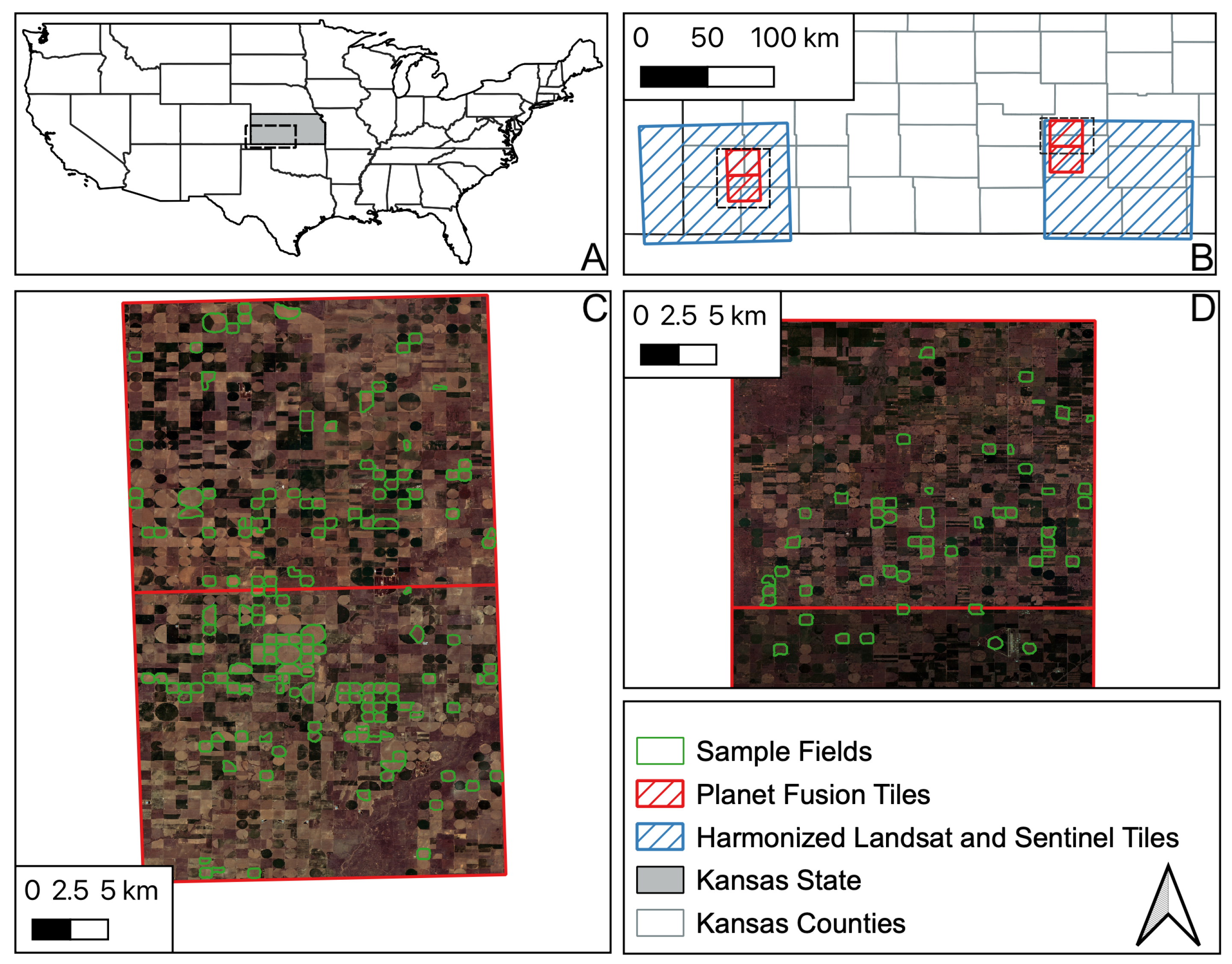
Figure 1. Location of fields contained in the Kansas State dataset and location of Planet Fusion tiles. (A) Location of sites in Kansas in the US. (B) Area of Planet Fusion and Harmonized Landsat Sentinel tiles for both sites in the Kansas dataset. (C) Western site field boundaries overlaid on Planet Fusion tiles and imagery. (D) Eastern site filed boundaries overlaid on Planet Fusion tiles and imagery.
Remotesensing 16 02730 g001
Figure 2. Maize phenology stages used during ground truth data collection in Kansas State. The scale follows that of Ciampitti et al. [38].
Remotesensing 16 02730 g002
Figure 3. Individual field-specific NDVI time series for all fields in the Kansas dataset before (left) and after cleaning (right).
Remotesensing 16 02730 g003
Figure 4. Number of observations in the Kansas dataset per micro- and macro-stage in chronological order, indication of pre-vegetative, vegetative and reproductive stages. In our study, we only consider vegetative stages starting from 1-leaf and reproductive stages.
Remotesensing 16 02730 g004
Figure 5. Histogram of BBCH phases of the observations in the PIAF dataset.
Remotesensing 16 02730 g005
Figure 6. Flow chart of data preprocessing and macro-stage identification with DTW.
Remotesensing 16 02730 g006
Figure 7. Planet Fusion NDVI time series for individual fields and average of all fields.
Remotesensing 16 02730 g007
Figure 8. Boxplot of median absolute errors (MedAEs) and mean absolute errors (MAEs) in days across 70 micro-stages for PF-NDVI, comparing three different methods.
Remotesensing 16 02730 g008
Figure 9. Variability of the RMSE in days for the selected micro-stages across different indices.
Remotesensing 16 02730 g009
Figure 10. NDVI time series of PF and HLS with predicted phenology dates for randomly selected micro-stages on two randomly selected fields.
Remotesensing 16 02730 g010
Figure 11. Comparison of the best PF and HLS DTW solutions for two macro-stages (comparison between observation DOY and predicted DOY). Orange and pink colors represent V4 and R1 macro-stages, respectively. Solid lines, dotted lines and dashed lines represent zero error, 5-day buffer and 10-day buffer. (a) Stage: V4 and R1; data: PF; index: MCARI. (b) Stage: V4 and R1; data: HLS; index: NDVI.
Remotesensing 16 02730 g011
Figure 12. Comparison of the best PF and HLS DTW solutions for three macro-stages (comparison between observation DOY and predicted DOY). Each row represents a different macro-stage where the left images are PF-based and the right ones are HLS-based predictions. Solid lines, dotted lines and dashed lines represent zero error, 5-day buffer and 10-day buffer. (a) Stage: R4; data: PF; index: MCARI. (b) Stage: R4; data: HLS; index: NDVI. (c) Stage: R5; data: PF, Index: MCARI. (d) Stage: R5; data: HLS; index: NDVI. (e) Stage: V8; data: PF; index: MCARI. (f) Stage: V8; data: HLS; index: MCARI.
Remotesensing 16 02730 g012aRemotesensing 16 02730 g012b
Figure 13. Outputs of the proposed method for four fields and macro-stages in Germany (ad). The dashed line indicates the observation in the PIAF dataset with the BBCH code, while ‘x’ marks represent the detected related micro-stages. Each vertical line represents one week.
Remotesensing 16 02730 g013
Table 1. Phenology stages for maize as used in the Kansas and PIAF datasets.
Macro-StageCorresponding
BBCH [39]
Starting
Micro-Stage
Ending
Micro-Stage
Number of
Micro-Stage
VEBBCH10EmergingSeedling—1 Leaf4
V1BBCH111-leaf1–2-leaf2
V2BBCH122-leaf2–3-leaf2
V3BBCH133-leaf3–4-leaf2
V4BBCH144 leaf4–5-leaf2
V5BBCH155-leaf5–6-leaf2
V6BBCH166-leaf6–7-leaf2
V7BBCH177-leaf7–8-leaf2
V8BBCH188-leaf8–9-leaf2
V9BBCH199-leaf9–10-leaf2
V10BBCH3110-leaf10–11-leaf2
V11N/A11-leaf11–12-leaf2
V12N/A12-leaf12–13-leaf2
V13N/A13-leaf13–14-leaf2
V14N/A14-leaf14–15-leaf2
V15N/A15-leaf15–16-leaf2
V16N/A16-leaf16-leaf—Tassel3
VTBBCH59TasselSilk—Brown Silk3
R1BBCH63SilkingSilking—Blister3
R2BBCH71BlisterBlister—Milk2
R3BBCH75MilkMilk—Dough2
R4BBCH85DoughDough—Early Dent4
R5BBCH86Early DentBlack Layer19
R6BBCH87MaturityMaturity1
Table 2. Vegetation indices.
IndexFormulaVegetation Property
NDVI(NIR − Red)/(NIR + Red)Productivity
EVI [41]2.5 × (NIR − Red)/((NIR + 6 × Red − 7.5 × Blue) + 1)Greenness
EVI2 [42]2.5 × (NIR − Red)/(NIR + 2.4 × Red + 1)Greenness
kNDVI [43]tanh(((NIR − Red)/(NIR + Red))2)Productivity
MCARI [44](1.2 × (2.5 × (NIR − Red) − 1.3 × (NIR − Green)))Leaf chlorophyll concentration
CVI [45]NIR × (Red/(Green2))Leaf chlorophyll content
NDWI [46](Green − NIR)/(Green + NIR)Water content
Table 3. Number (percentage) of observations detected with maximum errors of 1, 5, 10 and 15 days.
Max Error
Algorithm1 Day5 Day10 Day15 Day
Method 1486 (15%)1628 (50%)2550 (79%)3029 (94%)
Method 2652 (20%)1832 (57%)2645 (82%)2994 (93%)
Method 3 (proposed)636 (20%)2023 (63%)2900 (90%)3136 (97%)
Table 4. Performance of the proposed method based on NDVI and MCARI for some selected stages using PF. The bold font shows the best performance for each stage. Values for all phases are provided in Appendix A Table A1, Table A2, Table A3 and Table A4.
Phenology StagesRMSE (Days)MedAE (Days)MAE (Days)
MacroMicroNDVIMCARINDVIMCARINDVIMCARI
V11-leaf7.66.76.04.06.25.6
V44-leaf4.64.33.03.05.54.3
V44–5-leaf4.64.63.02.53.33.3
V66-leaf4.84.82.02.03.23.2
VTSilk—Brown Silk6.83.95.53.05.63.1
VTTassel7.25.16.04.06.54.3
VTTassel—Silk7.23.95.03.05.73.3
R1Pollen Shed6.95.85.03.05.54.3
R1Silking—Blister5.65.15.02.04.63.8
R52/3 Milk Line10.79.46.04.07.86.9
R5Early–Mid Dent6.37.84.56.04.86.4
R5Early Dent5.67.04.06.04.66.0
R5Full Dent7.38.75.06.05.86.6
R5Mid–Full Dent7.48.54.06.05.46.9
Disclaimer/Publisher’s Note: The statements, opinions and data contained in all publications are solely those of the individual author(s) and contributor(s) and not of MDPI and/or the editor(s). MDPI and/or the editor(s) disclaim responsibility for any injury to people or property resulting from any ideas, methods, instructions or products referred to in the content.