Construction of High-Precision and Complete Images of a Subsidence Basin in Sand Dune Mining Areas by InSAR-UAV-LiDAR Heterogeneous Data Integration

Abstract

Affected by geological factors, the scale of surface deformation in a hilly semi-desertification mining area varies. Meanwhile, there is certain dense vegetation on the ground, so it is difficult to construct a high-precision and complete image of a subsidence basin by using a single monitoring method, and hence the laws of the deformation and inversion of mining parameters cannot be known. Therefore, we firstly propose conducting collaborative monitoring by using InSAR (Interferometric Synthetic Aperture Radar), UAV (unmanned aerial vehicle), and 3DTLS (three-dimensional terrestrial laser scanning). The time-series complete surface subsidence basin is constructed by fusing heterogeneous data. In this paper, SBAS-InSAR (Small Baseline Subset) technology, which has the characteristics of reducing the time and space discorrelation, is used to obtain the small-scale deformation of the subsidence basin, oblique photogrammetry and 3D-TLS with strong penetrating power are used to obtain the anomaly and large-scale deformation, and the local polynomial interpolation based on the weight of heterogeneous data is used to construct a complete and high-precision subsidence basin. Compared with GNSS (Global Navigation Satellite System) monitoring data, the mean square errors of 1.442 m, 0.090 m, 0.072 m are obtained. The root mean square error of the high-precision image of the subsidence basin data is 0.040 m, accounting for 1.4% of the maximum subsidence value. The high-precision image of complete subsidence basin data can provide reliable support for the study of surface subsidence law and mining parameter inversion.

1. Introduction

Characterized by a shallow burial depth, thick coal seam, low hardness of surrounding rock, thick sandy soil-cap, etc., a coal mine in a sand dune area can easily induce different scales of deformation during the processes of large-scale and high-intensity mining. Due to the influence of special geology, the surface, and mining intensity, the use of a conventional observation station to obtain time-series subsidence data and analyze the subsidence law has gradually exposed certain deficiencies. Therefore, the use of modern surveying technology to construct a complete and high-precision image of a surface subsidence basin in a sand dune mining area has become a key point for studying spatio-temporal combinations and data fusion [1].

With the development of the space–sky–surface integrated monitoring technique, the three monitoring technologies of InSAR, UAV, and LiDAR have been greatly improved, and they all differ from each other. InSAR is an active microwave remote sensing technology, which is not affected by weather, and can be used for the periodic monitoring of large areas. UAV is a passive optical remote sensing technology with strong flexibility and a high resolution, and it can be used to obtain high-definition DOMs (Digital Orthophoto Maps) and a high-precision DEM (Digital Elevation Model). LiDAR is an active laser radar remote sensing technology with strong flexibility and penetrating ability, and it can be used for obtaining high-precision time-series DEMs by performing time-series monitoring in densely vegetated areas. Monitoring data with high precision can be obtained by using different technologies at different times and in different spaces. At the same time, this process can provide reliable technical support and data for the efficient, complete, and accurate construction of surface subsidence basin maps of sand dune mining areas.

With its extensive development, InSAR has gradually become a mature and cutting-edge Earth observation technology in the field of remote sensing. It can perform all-weather, wide-range, and long-time periodic continuous monitoring of surface subsidence. Many studies were conducted with InSAR, and it is widely used for the monitoring and analysis of earthquakes [2,3], volcanos [4,5], glaciers [6], urban planning [7,8], geological disaster identification [9], surface deformations [10], and many other fields. Due to the influence of surface vegetation, SAR images are prone to decoherence, hindering the extraction of real deformation data of the surface. Since improved InSAR, TCP-InSAR [11], SBAS-InSAR [12,13], PS-InSAR [14], and ITPA-InSAR [15] were used to extract high-coherent interference points, small-scale deformation at the edge of the subsidence basin in mining areas can be monitored accurately. In comparison to the leveling data, the accuracy can reach the millimeter level, and hence it is difficult to identify large-scale subsidence due to decoherence.

In order to monitor large-scale deformation, researchers studied the use of offset tracking [16], pixel tracking [17], and sub-band interferometry [18], among other technologies. Zhao et al. [19] used the offset tracking method of SAR to monitor large deformations. In view of the large gradient deformation of surfaces, Huang et al. [20] used normalized and correlation-maximized pixel tracking methods to solve the data of 11 TerraSAR-X images, where the RMSD (root mean square error) values of the data obtained by the improved method and GPS in the strike–inclination directions of the subsidence basin image data were 0.143 m and 0.108 m, respectively. Ou et al. [16] used D-InSAR and MTInSAR pixel offset tracking techniques to solve the data of 20 TerraSAR-X images. Combined with the spatial joint analysis function of ArcGIS, different solution data were fused, and the average absolute error was greatly reduced to 0.0748 m. High-resolution SAR images are necessary to obtain centimeter-level subsidence data.

UAVs are also developing rapidly and are specifically applied to geodetic mapping, photogrammetry, and disaster prevention and control strategies. Based on the combination of UAV remote sensing data and laser scanning data, some scholars in the field of ground motion monitoring used the above methods to observe horizontal and vertical displacements under the best monitoring conditions, and to study the creep and sliding characteristics of frozen soil [21,22]. Puniach et al. [23] used the orthophotomosaic technique to solve high-resolution image data obtained by UAV, followed by the improvement of the accuracy of the matching algorithm, and finally extracted the surface horizontal deformation data produced by coal mining. Ignjatović et al. [24] used a UAV to monitor the deformation in the Velenje coal mine and analyzed the accuracy of the monitoring data obtained by UAV, GNSS, and a total station, and the UAV was better for complex terrain areas. Ćwiąkała et al. [25] analyzed the instantaneous deformation law of a UAV in the mining area. Their study showed that the horizontal accuracy could reach 1.5-2GSD (ground sampling distance), and the accuracy in the vertical deformation could reach 2-3GSD. According to different studies, UAVs can be applied in the process of coal mining, but their accuracy will be affected by vegetation coverage. However, LiDAR can be used to solve this problem.

LiDAR has the characteristics of high precision, high efficiency, strong penetration, and obtaining multi-angle measurements. It can be used to obtain the spatial–temporal dynamic data of vegetation areas in hilly and dune mining regions. LiDAR, GNSS, and InSAR were used by Khan et al. [26] for the time-series analysis of surface subsidence caused by underground oil and gas exploitation. Dong et al. [27] combined airborne laser radar data with ground monitoring data and proposed a new registration method that effectively improved the surface deformation monitoring accuracy of the airborne laser radar data and verified the method’s feasibility in surface deformation monitoring. For surface temporal deformation induced by coal mining, Zheng et al. [28] adopted an airborne laser radar to determine 3D spatial point cloud data and the progressive triangular filtering algorithm to determine ground point cloud data. They constructed a subsidence model by using the data generated through the multi-period ground difference equation and obtained accuracy up to the centimeter level by comparing it with ground point cloud data. Combining the point cloud data obtained by airborne laser radar and optical data obtained by UAV, Zhu et al. [29] proposed the model-to-model cloud comparison (M3C2) algorithm based on 3D point cloud data to obtain real surface deformation data.

The complex terrain, thick and loose soil, and some vegetation in the hilly and dune mining areas make it difficult to set up and protect observation stations. A single measurement method could barely be used to collect time-series, high-precision, and high-quality subsidence data, and it is also difficult to obtain the overall subsidence law of a subsidence basin. In summary, the rapid development of modern measurement technology and data processing methods provides reliable theoretical and technical support for simultaneous time-series monitoring using a variety of technologies. In this paper, InSAR, UAV, and 3D terrestrial laser scanning (3DTLS) are used for coordinate monitoring, which can effectively and accurately construct surface subsidence basins in dune mining areas.

2. Materials and Methods

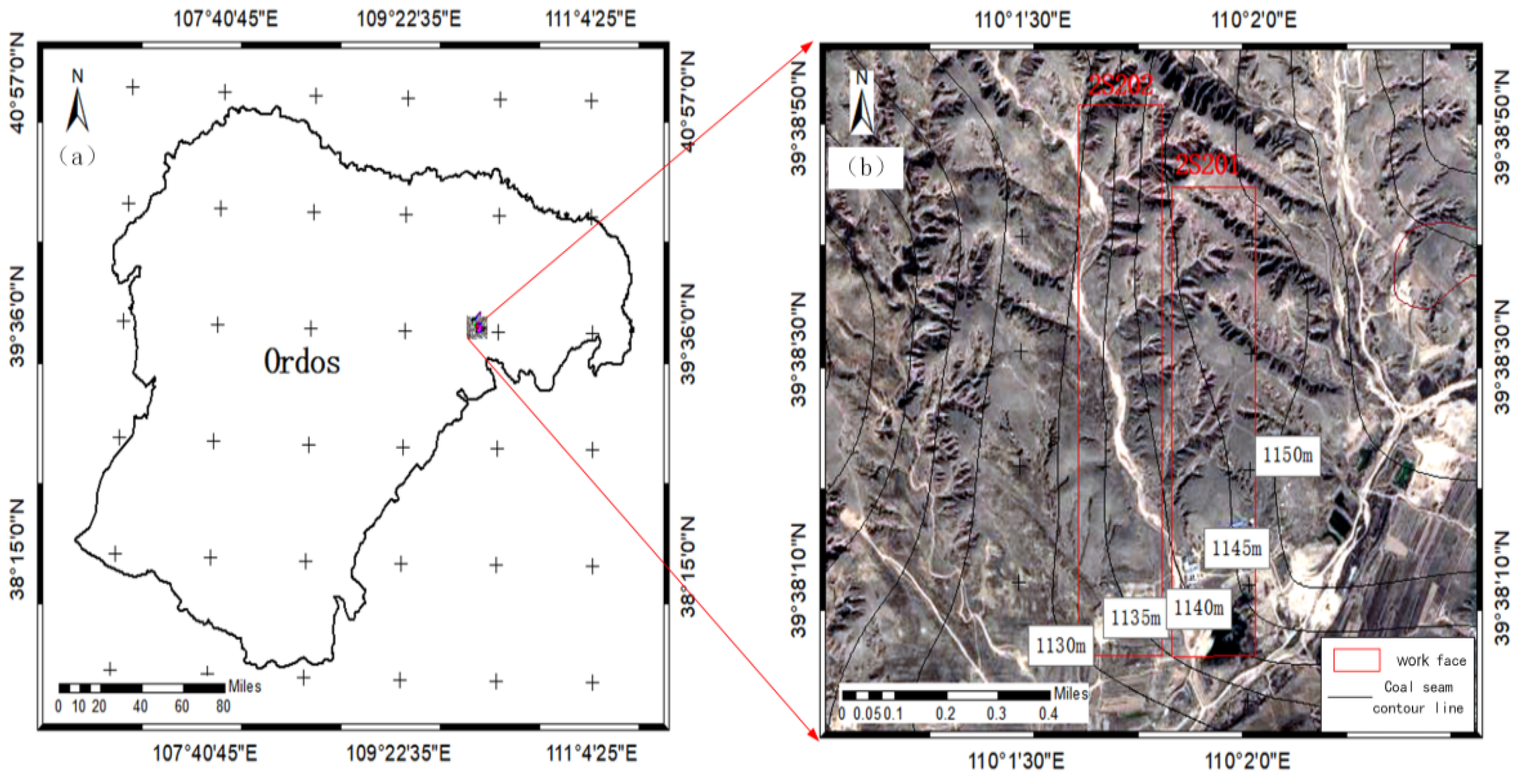
2.1. Study Area and Data

The research area taken as the main monitoring working surface is located in the field of the Wang Jiata mine in Erdos, Inner Mongolia, 2S201. The coal thickness in this region does not change a lot; it is between 2.9 and 3.5 m, with an average of 3.3 m. The specific research location is shown in Figure 1.

2.2. Data Acquisition

(1)

InSAR data

The experimental data for this work were collected from the combination of space–sky–surface integrated monitoring, which mainly includes InSAR, UAV, and LiDAR. The main SAR data used in the experiment are RadarSat-2 data (the Canadian Space Agency, Longier, QC, Canada and MDA Corporation, Brampton, ON, Canada), and the main parameters are listed in

Table 1. Parameters of RadarSat-2 images covering 2S201 and 2S202 working surfaces.

No.	Product	Beam Model	Polarization	Resolution/(m)	Acquisition Date	Pixel Center	Mean Incident Angle (°)
				(Rng × Az)		Lat–Lng (°)
1	SLC	Wide Multi-look Fine	HH	2.6 × 2.4	9 June 2018	39.5841–110.5944	35.2230
2					27 July 2018	39.5852–110.5950	35.2232
3					20 August 2018	39.5851–110.5961	35.2224
4					24 November 2018	39.591–110.5977	35.2128
5					11 January 2019	39.5892–110.5969	35.2129
6					4 February 2019	39.5627–110.5903	35.2124
7					28 February 2019	39.5729–110.5952	35.2165
8					24 March 2019	39.5899–110.5995	35.2207
9					17 April 2019	39.5880–110.5955	35.2223

.

(2)

UAV data

This time-series experiment was divided into four phases, all of which adopted the same image control point layout scheme and flight scheme, and also the same GNSS measurement method for measuring image control points and check points. According to the photogrammetry specification, combined with the terrain and accuracy requirements of the flight test area, both the fore-and-aft overlap rate and side overlap rate were set to 80%. In view of the area, shape, scale, and terrain change of the survey area, 8 image control points were evenly arranged in the survey area, and the coordinates of landmark points were measured by GNSS. Finally, the time-series DEM was obtained by photographic surveying. The aerial survey range, route, and image control point layout are shown in Figure 2.

Based on the ground sampling distance, the camera focal length was 15 mm and pixel size, the relative flying height of this experiment was 230 m, and the surface resolution was about 6 cm. The specific parameters are listed in

Table 2. Optical image acquisition parameters.

No.	UAV	Camera	Course Overlap%	Lateral Overlap%	Ground Resolution (m)	Row Height (m)	Collection Date
1	Trimble UX5	SONY A5100	80	80	0.06	230	9 June 2018
2							4 September 2018
3							16 October 2018
4							16 April 2019

.

(3)

LiDAR data

A 3D laser scanner was used for time-series monitoring in the key and dense vegetation areas of the surface deformation law of the hilly sand dune mining area. Figure 3 shows a schematic diagram of the surface deformation extracted by the 3D laser scanning in the process of surface subsidence monitoring. When the working face advanced to position 1, the first scan was performed, and the surface data were extracted to construct the subsidence area DEM1. When the working face advanced to position 2, the scan was performed again to obtain DEM2. By subtracting DEM1 and DEM2, the actual surface subsidence between the two periods of mining in the monitoring area can be obtained.

A Reigl VZ-1000 Laser Scanner was used to monitor the 2S201 working face of the mining area and collect experimental data. Data were collected only from the southern area of the 2S201 working face. The station layout is shown in Figure 4.

According to the area of the 2S201 working face, topography, vegetation, and buildings, S1 to S16 scanning points were set up in the central and southern parts of the working face. A total of 4 times of data were collected during the mining period from June 2018 to October 2018. After the subsidence stabilized, the last observation was conducted in April 2019; i.e., a total of 5 times of the 3D point cloud data were collected during the whole monitoring process of the mining of the 2S201 working face.

2.3. Principle of SBASInSAR Technology

It is assumed that there are N + 1 radar images of the same area, arranged in order of time series (t₀, t₁, …, t_N), and that each image is at least paired with one other image for differential interferometry. The number of differential interferograms is M, which conforms to Equation (1).

$${\displaystyle \frac{N+1}{2}}⩽M⩽N{\displaystyle \frac{N+1}{2}}$$

(1)

Suppose that the jth interferogram comes from two images at time instants t_B and t_A, the terrain phase part of the point in the interferogram is removed, and some decoherence phenomena, atmospheric refraction, DEM error, and other interference phases are temporarily ignored. Then,

$$\delta {\phi }_j=\phi \left(t_B\right)-\phi \left(t_A\right)\approx {\displaystyle \frac{4\pi }{\lambda }}\left[d\left(t_B\right)-d\left(t_A\right)\right]$$

(2)

In Equation (2), λ is the central wavelength, and d(t_B) and d(t_A) are the cumulative deformation of the line of sight (LOS) at t_B and t_A, respectively. Taking t₀ as the reference, d(t₀) = 0 = 0 is obtained. For i = 1, 2, ..., N, suppose that the time series is deformed to φ(t_i), which is the phase part of the correlation. Then, it comes to φ(t_i) ≈ 4πd(t_i)/λ.

It is assumed that φ(t_i) is the unwrapped phase, and it is corrected by the unwrapped phase error and far field or control point. Firstly,

$${\phi }^{\mathrm{T}}=\left[\phi \left(t_1\right),\phi \left(t_2\right),\cdots ,\phi \left(t_N\right)\right]$$

(3)

It is an N-dimensional vector, representing the unknown phase value associated with deformation. Then,

$$\delta {\phi }^T=\left[\delta {\phi }_1,\delta {\phi }_2,\cdots ,\delta {\phi }_M\right]$$

(4)

It is an M-dimensional vector, representing a known value.

In order to avoid large discontinuous cumulative deformation and prevent the results obtained with no physical significance, SBAS generally adopts a piecewise linear algorithm. If the phase unknowns are replaced with the average phase velocity of the image time interval, the new unknowns can be expressed by Equation (5).

$$v^{\mathrm{T}}=\left[v_1,v_2,\cdots ,v_N\right]=\left[{\displaystyle \frac{{\phi }_1}{t_1-t_0}},{\displaystyle \frac{{\phi }_2-{\phi }_1}{t_2-t_1}},\cdots ,{\displaystyle \frac{{\phi }_N-{\phi }_{N-1}}{t_N-t_{N-1}}}\right]$$

(5)

Substituting Equation (5) into Equation (2), we can obtain

$${\displaystyle \sum _{k=1S_j+1}^{I{E}_j}\left(t_k-t_{k-1}\right)}{v}_k,\hspace{1em}\forall j=1,2,\cdots ,M$$

(6)

Therefore, a new matrix system is formed, and the final expression is given by Equation (7).

$$Bv=\delta \phi$$

(7)

where B is another M × N matrix, but now (j, k) elements are set. When IS_j + 1 ≤ k < IE_j, $\forall$_j = 1, 2, …, M, B(j,k) = t_k + 1 − t_k; otherwise, B(j, k) = 0.

A large number of data are used to generate a small baseline interferogram set, so as to obtain the deformation of the time series of each subset. However, there will be a problem with different interferogram subsets having no common image. Using SVD to transform it into a subset problem, the minimum norm criterion can be used to estimate the deformation, and subsequently, the deformation information can be obtained.

2.4. Principle of UAV Technology

The imaging equation of a UAV image is the mathematical relationship between the image coordinates (x, y) of the ground object points on the image and the geodetic coordinates (X, Y, Z) of the corresponding points on the ground. This mathematical relationship is the basis for geometric correction of any type of transmitter imaging and error analysis of some parameters.

In order to establish the mathematical relationship between the image points and the corresponding ground points, it is necessary to establish a coordinate system like the object space, as shown in Figure 5.

All of the above coordinate systems represent three-dimensional space. The most basic coordinate systems are the image coordinate system oxy and map coordinate system (O_m, X_m, Y_m). These are two-dimensional plane coordinate systems, whose starting point and final aim are the geometric processing of remote sensing images.

The transformation relationship between the ground coordinate system and sensor coordinate system is called the general imaging equation. Assuming that the coordinate of the ground point P in the ground coordinate system is (X, Y, Z)p, the coordinate of P is (U, V, W)p, the coordinate of the sensor projection center S is (X, Y, Z)s, and the attitude angles of the sensor are φ, ω, Κ, their general imaging can be expressed by Equation (8).

$${\left[\begin{array}{l}X\hfill \\ Y\hfill \\ Z\hfill \end{array}\right]}_P={\left[\begin{array}{l}X\hfill \\ Y\hfill \\ Z\hfill \end{array}\right]}_s+A{\left[\begin{array}{l}U\hfill \\ V\hfill \\ W\hfill \end{array}\right]}_P$$

(8)

In Equation (8), A is the rotation matrix of the sensor coordinate system relative to the ground coordinate system. It is a function of φ, ω, Κ, in the sensor attitude angle, and is a known parameter. Through this model, the three-dimensional coordinates of the center point of each pixel in the monitoring range can be solved to obtain the time-series DEM, and then the subsidence basin can be obtained.

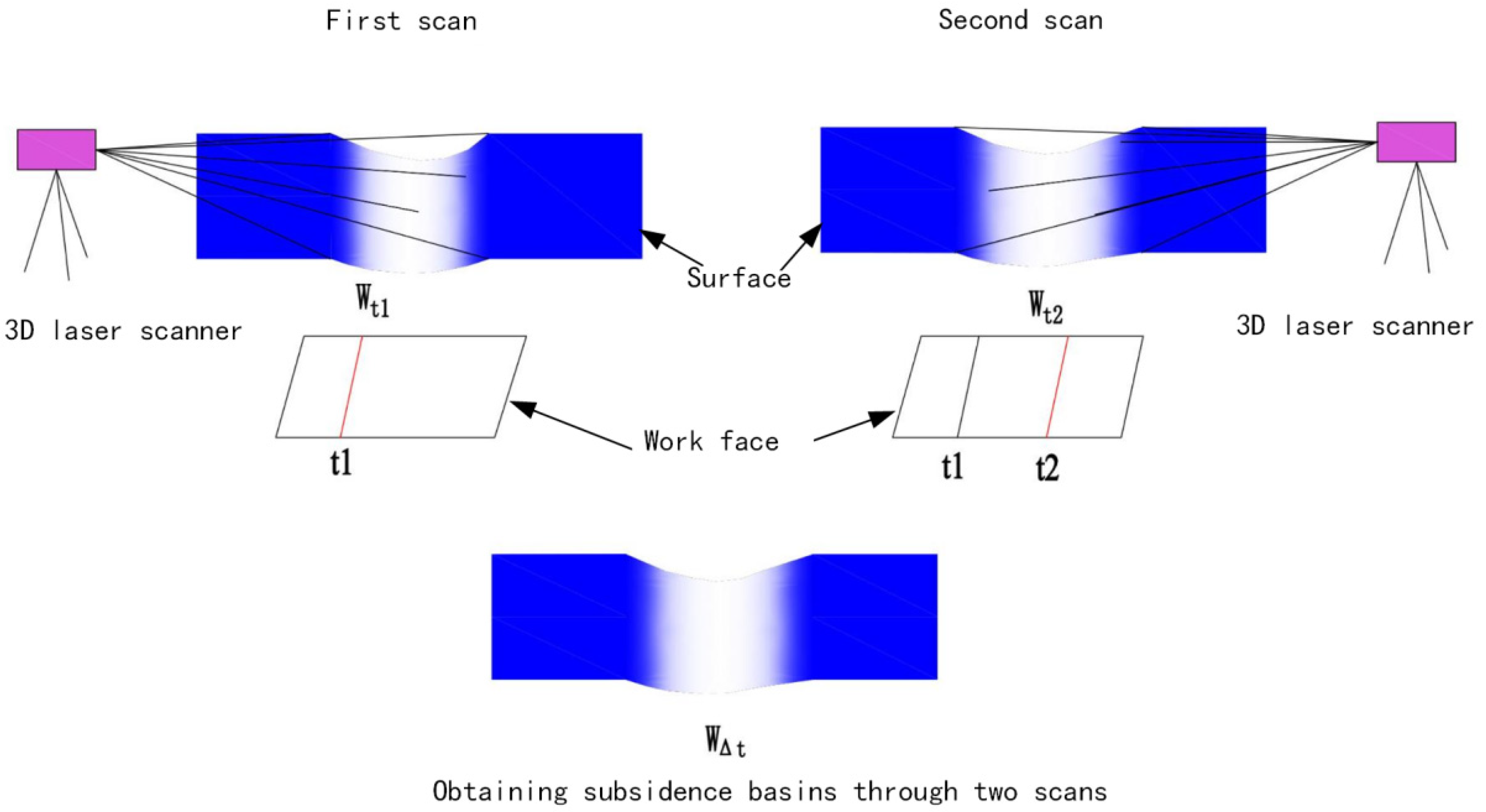
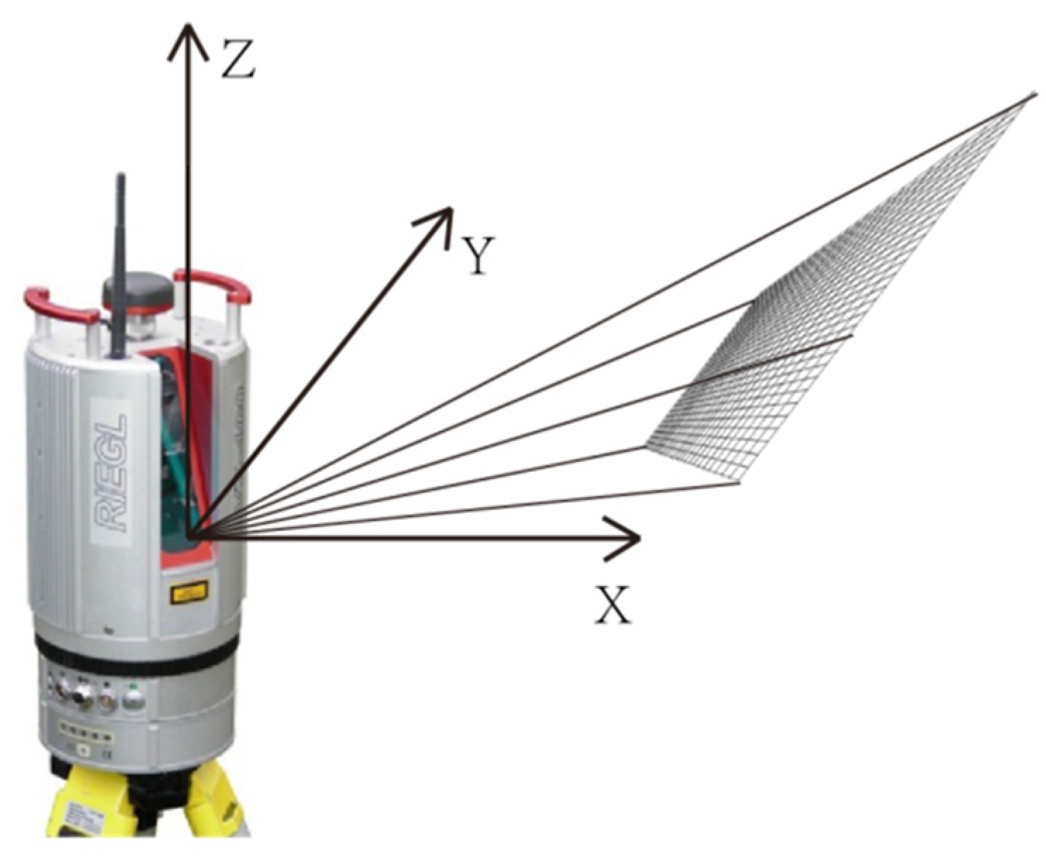
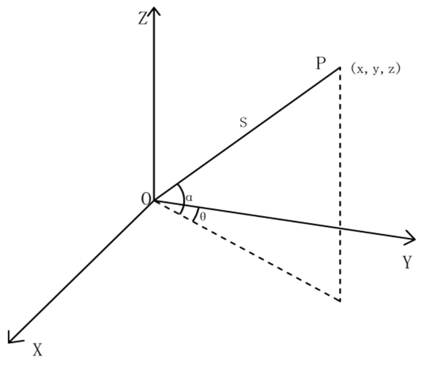
2.5. Principle of LiDAR Technology

The basic principle of the 3D laser scanning technology is the laser ranging, which can quickly emit laser in a short period of time, so as to obtain massive 3D point cloud coordinate data of a target. During the operation, the laser rapidly emits a laser beam, which is reflected back immediately when it contacts the target and is received by the receiver. At the same time, the timer records the time of emission and reception by the laser and receiver, respectively, and calculates the distance from the laser emission center to the target through the laser speed. Finally, the three-dimensional space coordinates of the laser-measured points in the rectangular coordinate system are obtained through the horizontal and vertical angles of the scanner recorded by the encoder. This principle is depicted in Figure 6.

Point O in Figure 7 is the laser beam emission center. The three-dimensional space coordinates of this point can be obtained by observation. During the scanning process, the laser beam emitted from Point O is scanned horizontally and vertically along the X, Y, and Z axes. Let S be the distance from the laser emission center to the measured target calculated by a precision timer, and the horizontal angle θ and vertical angle α are recorded in combination with the internal control encoder of the scanner. The three-dimensional space coordinates of Point P can be expressed by Equation (9).

$$\left\{\begin{array}{l}X=S\cdot \cos a\cdot \sin \theta \\ Y=S\cdot \cos a\cdot \cos \theta \\ Z=S\cdot \sin a\end{array}\right.$$

(9)

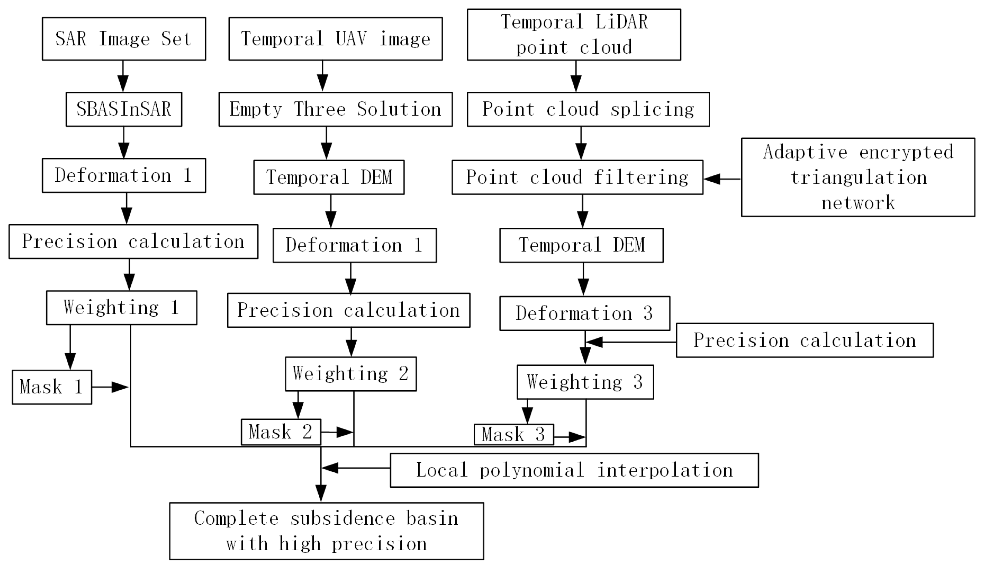
2.6. Data Fusion Theory

For heterogeneous data fusion, any fusion method will have a certain impact on the data accuracy. It is assumed that the fused data are composed of two types of data, one having a weight of P and the other of (1 − P), so that there is no deviation in the fusion. The variance model after fusion by the law of error propagation can be expressed by Equation (10).

$${\sigma }_{\mathrm{merge}}^2=P^2{\sigma }_1^2+{(1-P)}^2{\sigma }_2^2+2kP{\sigma }_1(1-P){\sigma }_2$$

(10)

In Equation (10), P is the first data weight, (1 − P) is the second data weight, k is the correlation coefficient of the two data sets, and σ₁ and σ₂ are the standard deviations of the two data sets, respectively. The weight P should minimize the overall error of the fused data, specifically to minimize ${\sigma }_{\mathrm{merge}}^2$, i.e., to obtain the minimum value of ${\sigma }_{\mathrm{merge}}^2$ by making the derivative P equal to 0, which is simplified as in Equation (11).

$$\begin{array}{l}P={\displaystyle \frac{{\sigma }_2^2-k{\sigma }_1{\sigma }_2}{{\sigma }_1^2+{\sigma }_2^2-2k{\sigma }_1{\sigma }_2}}\\ ={\displaystyle \frac{1}{2}}(1+{\displaystyle \frac{{\sigma }_2^2-{\sigma }_1^2}{{\sigma }_1^2+{\sigma }_2^2-2k{\sigma }_1{\sigma }_2}})\end{array}$$

(11)

In docking fusion, the correlation between the two data sets is minimal, and assuming k is 0, Equation (12) is obtained.

$$P={\displaystyle \frac{{\sigma }_2^2}{{\sigma }_1^2+{\sigma }_2^2}}$$

(12)

For Equation (12), σ_i can be computed using Equation (13).

$${\sigma }_i=\sqrt{{\displaystyle \frac{{(x_1-x)}^2+{(x_2-x)}^2+{(x_3-x)}^2+\cdots {(x_i-x)}^2}{i-1}}}$$

(13)

In Equation (13), σ_i is the standard deviation, x_i is the observation of InSAR, UAV, or LiDAR, and x is the true value of observation.

It can be seen that ${\sigma }_{\mathrm{merge}}^2$ is not greater than the data with the smaller variance. Before the fusion, the weight of the two data sets is unknown. As their relative contributions increase, k changes. It can be seen from Equation (10) that when the two data sets are overlapped and fused, the correlation coefficient and weight increase with an increase in the number of fusion points. When the deformation data are spliced, the weight of high-precision data becomes the smallest. Therefore, the accuracy of the final fusion data becomes the highest upon the superposition of the overlapping and fusion data. The accuracies of SBASInSAR, UAV, and LiDAR data in subsidence monitoring are obtained from previous experiments and also from this work. A local polynomial is used to assign different weights to the data according to the accuracy for further fusion [30].

In this paper, the local polynomial interpolation method is improved, and different data weights are fused. The interpolation accuracy is most sensitive to the neighborhood distance. The neighborhood search radius is set according to the actual needs. So, the interpolation can be predicted even if the neighborhood is small. This interpolation method performs a non-parametric estimation with a kernel function. From the theoretical point of view, it has good estimation performance and is widely used in practice. In the overlapping area of the data fusion, local polynomials can be fitted by multiple polynomials. Efficient and high-precision interpolation can be obtained by setting parameters, such as the size, shape, function model selection, goodness of fit, and number of neighborhoods of the search neighborhood. Alternatively, the number of synchronous space conditions, bandwidth, and search radius of parameters can be analyzed using the exploratory trend surface analysis, and parameters for local polynomial interpolation can be obtained by optimizing statistical functions obtained by the cross-validation method.

In the local polynomial model, pⁿ(x) is assumed to be the nth derivative of the regression function p(x) in Y_t = p(X_t) + q(X_t)ε_t. The local polynomial model can be used to estimate pn(x) more efficiently and conveniently, and the regression function p(x) = p₀(x) is the same. Since the regression function is not determined, the data points far away from x₀ in the estimation process have little influence on p(x₀). Therefore, in the process of estimation, only the proximal point of x₀ is used to estimate p(x₀), which is more reasonable. Suppose that p(x) has n + 1 order derivative at x₀, and x is expanded by Taylor’s formula about the local region of x₀. Then, the model can be expressed by Equation (14).

$$\begin{array}{l}p(x)=p\left(x_0\right)+p^{\prime }\left(x_0\right)\left(x-x_0\right)+{\displaystyle \frac{p^{″}\left(x_0\right)}{2!}}{\left(x-x_0\right)}^2+,L,+\\ +{\displaystyle \frac{p^{(n)}\left(x_0\right)}{n!}}{\left(x-x_0\right)}^n+O\left\{{\left(x-x_0\right)}^{n+1}\right\}\end{array}$$

(14)

The x₀ local area point cloud p(x) is modeled, as given by Equation (15).

$$p(x)\approx {\displaystyle \sum _{i=0}^n{\beta }_i}{\left(x-x_0\right)}^i$$

(15)

In Equation (15), parameter β_i is mainly related to x₀. So, it is a local parameter.

According to Equations (14) and (15), the local parameter β_n = m(n)(x₀)/n! can be used to fit the local model as expressed by Equation (16).

$${\displaystyle \sum _{t=1}^T{\left\{Y_t-{\displaystyle \sum _{i=0}^n{\beta }_i}{\left(X_t-x_0\right)}^i\right\}}^2}{K}_h\left(X_t-x_0\right)$$

(16)

In Equation (16), K_h is the weight function, also known as the kernel function, and h is the broadband size of the local neighborhood. The local polynomial regression equation is expressed as a matrix as given by Equation (17).

$$\begin{array}{l}X=\left(\begin{array}{ccc}1& \left(X_1-x_0\right)\cdots & {\left(X_1-x_0\right)}^n\\ ⋮& ⋮& ⋮\\ 1& \left(X_T-x_0\right)\cdots & {\left(X_T-x_0\right)}^n\end{array}\right),\\ Y=\left(\begin{array}{c}{Y}_1\\ ⋮\\ Y_T\end{array}\right),\hspace{1em}\widehat{\beta }=\left(\begin{array}{c}{\widehat{\beta }}_0\\ ⋮\\ {\widehat{\beta }}_n\end{array}\right)\end{array}$$

(17)

The ordinary least square is used to rewrite Equation (17) as in Equation (18).

$${\min }_{\beta }{(Y-X\beta )}^{T}R(Y-X\beta )$$

(18)

In Equation (18), β = (β₀, ……, β_n)^T, R is diagonal matrix, the ith element is K_h(X_i − x₀), and the solution vector is given by Equation (19).

$$\widehat{\beta }={\left(X^{T}RX\right)}^{-1}{X}^{T}RY$$

(19)

According to Equation (19), when the estimated interpolation result is p_n(x), then p_z(x₀) = β_n.

The continuous mining of coal resources leads to the use of more diversified monitoring methods for surface deformation. The obtained surface deformation data formats also vary a lot. Due to different monitoring methods, different sensors, and different data processing methods, the accuracy of the final deformation monitoring data is different. This paper proposes that in the case of considering data accuracy, the data fusion can be performed after weighting according to accuracy, and subsequently a more complete and high-precision subsidence basin can be obtained. The technical flow chart is shown in Figure 8.

3. Results

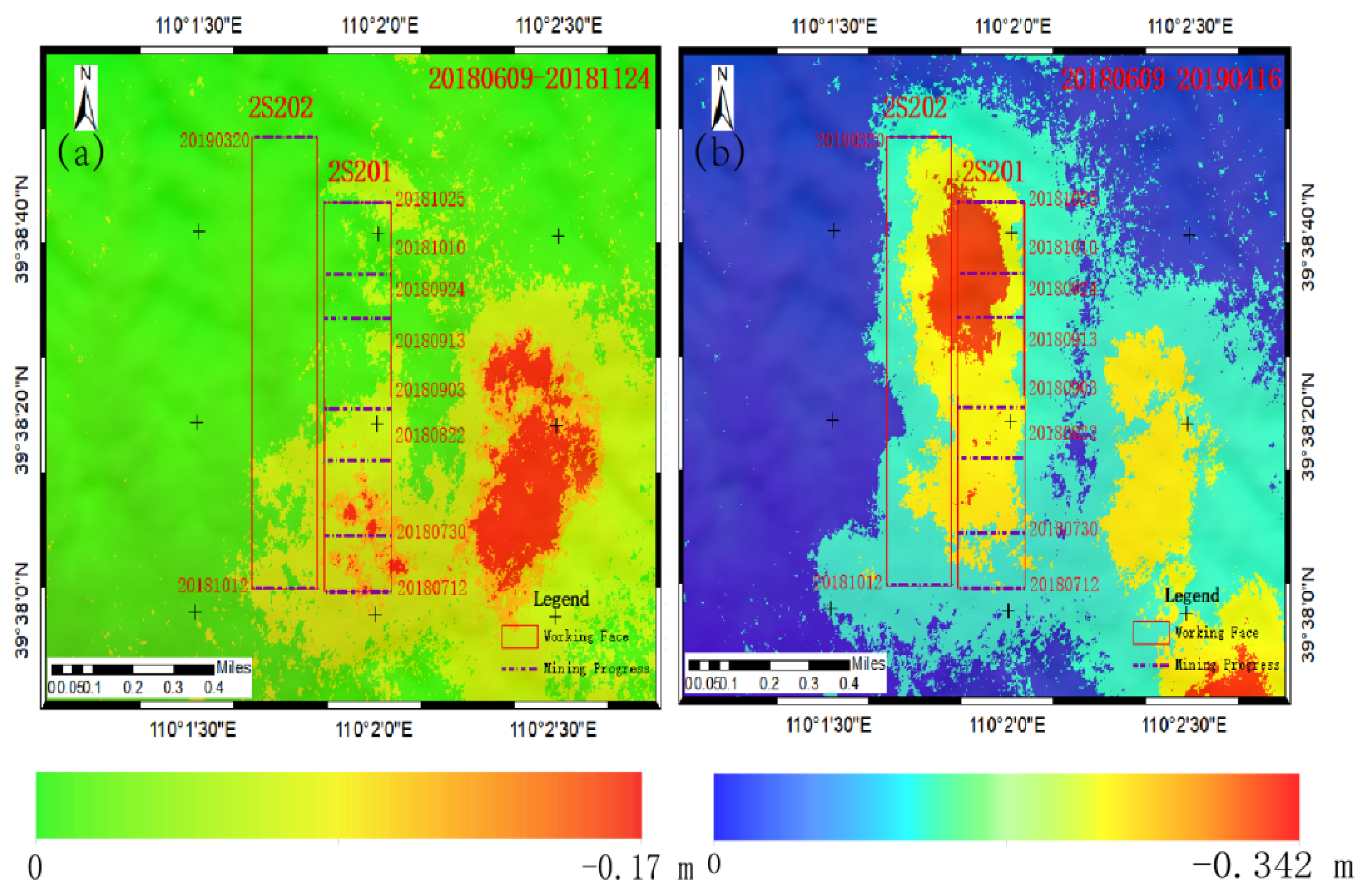
3.1. Results of SBASInSAR

For a repeat-pass interferogram, the interferometric phase is related to the selected reference ellipsoid, the position of the ground point, whether the ground surface is deformed and the scale of the deformation, the atmospheric delay error and the noise of the SAR system [31]. The interference phase model can be expressed by Equation (20).

$$\varphi ={\varphi }_{flat}+{\varphi }_{topo}+{\varphi }_{defo}+{\varphi }_{orbit}+{\varphi }_{atm}+{\varphi }_{noise}$$

(20)

In Equation (20), ${\varphi }_{flat}$ represents the reference ellipsoid phase, ${\varphi }_{topo}$ is the terrain phase, ${\varphi }_{defo}$ is the deformation phase along the line of sight (LOS), ${\varphi }_{orbit}$ is the phase caused by orbital error, ${\varphi }_{atm}$ is the atmospheric delay phase, and ${\varphi }_{noise}$ is the phase caused by noise. An external high-precision DEM is mainly used to eliminate terrain interference phase error. In this experiment, the external DEM is fused with the high-precision DEM obtained by UAV and the DEM obtained by SRTM to obtain a high-precision DEM in the study area.

The small magnitude of settlement in the initial stage of subsidence can accurately identify the surface deformation and range. However, as the magnitude of subsidence in mining increases with time, it is difficult to identify more accurate subsidence. The main reason is that the magnitude of surface subsidence in this period is large, and the spatial decoherence is serious, which cannot be untangled correctly, but the boundary of the subsidence basin can be extracted as shown in Figure 9.

Figure 9 shows that the SBASInSAR technology can be applied to identify the boundary of 10 mm surface deformation, where the maximum cumulative subsidence value is 0.342 m. Compared with the UAV recognition results, the maximum real subsidence is quite different. The SBASInSAR technique is not suitable for large-scale subsidence monitoring, but it can be used to identify the boundary of a subsidence basin well.

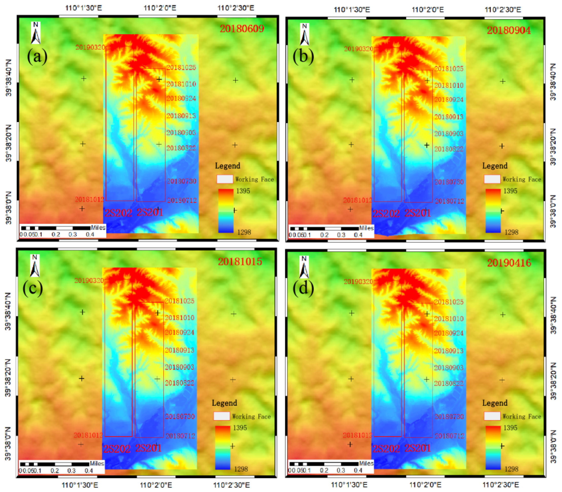
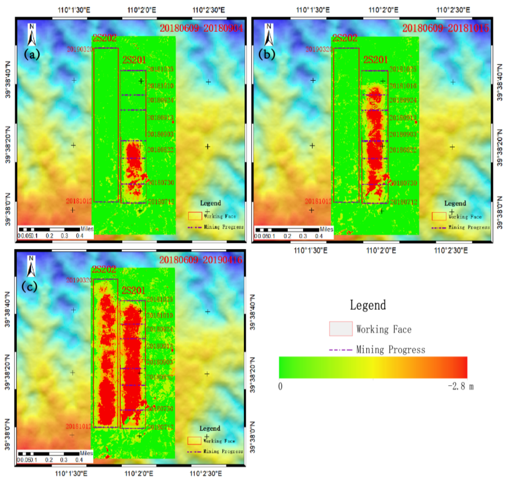
3.2. UAV Results and Accuracy Analysis

In the process of data acquisition, the theoretical models of flight height, photography baseline, and route interval setting are given by Equations (21)–(23), respectively. The data acquisition and flight plan are formulated according to the actual situation of terrain and structures, as expressed by Equation (21).

$$\mathrm{H}={\displaystyle \frac{f\times \mathrm{GSD}}{a}}$$

(21)

In Equation (21), a is the pixel size, H stands for the photographic flight height, GSD is the ground resolution, and f is the lens focal length.

$$\begin{array}{l}{b}_X=L_X\left(1-p_X\right)\hfill \\ d_X=L_Y\left(1-q_Y\right)\hfill \end{array}$$

(22)

$$\begin{array}{l}{B}_X=b_X\times {\displaystyle \frac{\mathrm{H}}{f}}\hfill \\ D_Y=d_Y\times {\displaystyle \frac{\mathrm{H}}{f}}\hfill \end{array}$$

(23)

In Equations (22) and (23), b_X and d_Y are the width of the route interval and length of the photographic baseline on the image, respectively; D_Y and B_X are the width of the route interval and length of the photographic baseline on the spot, respectively; and L_Y and L_X are width and length of the image, respectively. In the image, p_X is the heading, q_Y is the side direction, f is the focal length of the camera, and H is the height of flight photography.

According to the actual field situation, combining Equations (21)–(23), the flight plan is formulated with a ground resolution of 0.06 m, flight height of 230 m, and heading and lateral overlap of 80%. According to the above flight plan, a total of four UAV photogrammetry images of the 2S201 working face are obtained, and the time-series DEM is constructed, as shown in Figure 10.

Figure 10a shows the undeformed DEM surface before the start of mining the 2S201 face, Figure 10b,c show the time-series deformations of the DEM surface during the mining period, and Figure 10d shows the DEM surface after mining for 6 months with stable subsidence. In an analysis of Figure 10, it is found that the terrain of this working face is more complex and undulating with more gullies, low in the south with more vegetation, and high in the north. If the traditional method was used to monitor and analyze the subsidence law, it would have been impossible to set up the observation station in strict accordance with the “coal pillar and mining regulations of buildings, water, railways and main roadways”, issued by the China National Coal Association and difficult to ensure the integrity, timing, and accuracy of the data.

According to the root mean square error model expressed by Equation (24), the root mean square errors in the time-series DEM of the four periods were calculated, as presented in

Table 3. Timing DEM accuracy.

Date	20180609	20180904	20181015	20190416	Mean Squared Error in Average Observation (m)
Mean Square Error of Observation (m)	0.101	0.118	0.109	0.091	0.105

.

$$\mathrm{M}=\pm \sqrt{{\displaystyle \frac{{\displaystyle \sum _{i=1}^n{\left[\nu \nu \right]}_i}}{n-1}}}$$

(24)

In Equation (23), M is the root mean square error, n is the number of calculated points, ν is the difference between the GNSS monitoring data and UAV-DEM monitoring data.

Due to the influence of seasons, when the data were collected in the fourth phase, the surface vegetation was less than that in the other three phases. Therefore, the accuracy of the DEM model solved using the data in 20190416 is the highest, with a root mean square error of 0.091 m. It can be concluded that the surface vegetation has a certain influence on the image and construction of a high-precision DEM. Based on the constructed surface space DEM of the four time series before and after mining of the 2S201 working face, the time-series subsidence basin of the working face is extracted, as shown in Figure 11.

Figure 11 shows the time-series subsidence basin extracted from the four phases of the surface DEM collected from the 2S201 working face in the period from 9 June 2018 to 16 April 2019. Figure 11a–c show the time-series dynamic subsidence basin images. The areas with large subsidence magnitude are mainly concentrated in the central area of the working face, and the effect of vegetation on the southern area is poor. According to the root mean square error model given by Equation (24), 12 test points were selected to calculate the root mean square error of the time-series subsidence basin, as presented in

Table 4. Accuracy of UAV time-series subsidence basin.

Data	20180904	20181015	20190416	Mean Square Error
Error in settlement (m)	0.091	0.098	0.091	0.093

.

The experimental results show that the UAV photogrammetry technology can be used to monitor large-scale surface subsidence. The minimum, maximum, and average root mean square errors of subsidence observation are 0.091 m, 0.098 m, and 0.093 m, respectively. The maximum surface subsidence after mining for the purpose of stabilization is 2.78 m. The UAV photogrammetry technology could effectively identify the central subsidence range of the subsidence basin. However, it was difficult to accurately identify the edge area of the subsidence basin and also to obtain the complete subsidence basin.

3.3. LiDAR Results and Accuracy Analysis

In the process of data acquisition by the 3D laser scanning technology, the collected 3D point cloud data contain some noise, which affects the construction of a high-precision surface DEM. So, these data need to be filtered. This paper proposes improving the adaptive grid progressive TIN densification filtering encryption algorithm. By improving the accuracy of the seed points, the accuracy of the irregular triangulation network can be improved, so as to judge the points accurately. Finally, the accuracy of the filtering algorithm is improved. This model is completed in C# programming language. The principle is shown in Figure 12.

In Figure 12, A₁(x₁,y₁,z₁), A₂(x₂,y₂,z₂₎, and A₃(x₃,y₃,z₃) are the three vertices of any triangle in the triangle irregular network; point A(x₀,y₀,z₀) is the internal judgment point of the triangle; d is the vertical distance between point A and the plane of the triangle; and δ₁, δ₂, and δ₃ are the plane angles of the lines between point A and the three vertices of the triangle, respectively. The triangular plane model is expressed by Equation (25).

$$ax+by+cz+d=0$$

(25)

The vertical distance d from the judgment point A(x₀,y₀,z₀) to the plane of the triangle is expressed by Equation (26), and the judgment angle δi is given by (27).

$$d={\displaystyle \frac{\left|a{x}_0+b{y}_0+c{z}_0+d\right|}{\sqrt{a^2+b^2+c^2}}}$$

(26)

$$\begin{array}{c}{\delta }_{\mathrm{i}}={\sin }^{-1}{\displaystyle \frac{\mathrm{d}}{{\mathrm{s}}_{\mathrm{iA}}}},\mathrm{i}=1,2,3\\ S_{iA}=\sqrt{{\left(x_{Ai}-x_A\right)}^2+{\left(y_{Ai}-y_A\right)}^2+{\left(z_{Ai}-z_A\right)}^2},i=1,2,3\end{array}$$

(27)

The improved AMR progressive encryption TIN filtering algorithm can be divided into two main parts. Firstly, AMR is established by using 3D point cloud data according to terrain features, and the threshold of the points in AMR is set to four according to the point cloud density and terrain. When the number is less than four, the lowest point is selected as the horizon. Secondly, if there are four points in AMR, three of which fit the surface, then the division efficiency can be increased by keeping the lowest point fixed. Its principle is shown in Figure 13.

The vertical angle δ_i and vertical distance d comprehensively reflect the degree of the triangular mesh protrusion. The smaller the vertical angle, the smaller the degree of protrusion, the smaller the degree of interference, and the higher the accuracy of surface points. The vertical distance can be a limitation in that when the triangulation network is large, the triangulation network does not produce any large jump. The adaptive grid progressive TIN densification filtering encryption algorithm establishes an irregular triangulation by dividing precise triangles. On this basis, the precise seed points are extracted. By comparing the triangulation angle and vertical distance between the judge point and seed point, the surface points are extracted precisely. When the terrain is more complex, it usually requires more iterations each time to obtain a more accurate lowest point and update the iteration distance and iteration angle, so as to obtain the surface point, and the number of iterations in the flat area is less. The principle is shown in Figure 14.

Figure 14a shows the original surface point cloud data, Figure 14b shows the result of the Morphological Filtering Method, Figure 14c shows the result of CSF, and Figure 14d shows the result of the adaptive grid progressive TIN densification filtering encryption algorithm. From Figure 14, we can determine that the ground points obtained by using morphology and CSF in big rolling areas are uneven, and the point cloud data are especially rare in sparse vegetation areas. While the seed point can be chosen accurately by using the adaptive grid progressive TIN densification filtering encryption algorithm, the even and complete surface points can be extracted at a custom threshold and, most of all, improve the precision of surface deformation analysis.

By accurately obtaining the three-dimensional point cloud of the ground, high-precision time-series DEM data are established, and then the subsidence basin is extracted as shown in Figure 15.

Sixteen 3D laser scanning observation stations were set up above the 2S201 working face to conduct targeted experiments on 3D point cloud data acquisition. Through the data processing in the form of point cloud splicing, filtering, masking, and constructing a time-series DEM, the time-series subsidence basin in the central and southern part of the 2S201 working face is finally obtained, as shown in Figure 13. According to the data accuracy, the mask processing is carried out around the basin. The maximum subsidence in the center of the subsidence basin was found to be 2.78 m. Twelve test points were randomly selected, and the error model given by Equation (23) was used to calculate the time-series root mean square error. The obtained results are presented in

Table 5. Accuracy of LiDAR time-series subsidence basin.

Data	20180730	20180903	20181016	20190416	Mean Square Error
Error in subsidence basin (m)	0.066	0.065	0.068	0.077	0.069

.

It can be seen from Table 5 that the minimum, maximum, and average root mean square errors of the subsidence basin monitoring were 0.065 m, 0.077 m, and 0.069 m, respectively. The maximum and relative maximum subsidence errors were 2.78 m and 2.53%, respectively.

3.4. Fusion Results of Space–Sky–Surface Integrated Monitoring Data

The space–sky–surface integrated monitoring is used to monitor the study area at the same time, and the obtained subsidence basin data are weighted according to the data accuracy. In combination with the local polynomial interpolation method, data fusion is performed in MATLAB. The high-precision complete subsidence basin image, which was monitored from the beginning of mining on the 2S201 working face until stable subsidence, is obtained. The results are shown in Figure 16.

Figure 14 shows the surface stable subsidence of the working face for the period from July 2018 to April 2019. This method could accurately construct a complete subsidence basin, identifying the 10 mm mining influence boundary of the outer edge of the subsidence basin, where the maximum subsidence value was found to be 2.78 m. The experiment proves that through the collaborative monitoring of InSAR, UAV, and LiDAR, a relatively complete subsidence basin can be extracted, which provides reliable field-measured data for studying the mining subsidence law and parameter inversion.

4. Discussion

Comparative Analysis of Data Obtained from InSAR, UAV, LiDAR, and GNSS

In order to ensure accuracy, the corresponding verification points were arranged on the site, and the space–sky–surface integrated monitoring data were collected. Due to the large surface fluctuation in the research area, GNSS was mainly used for time-series monitoring. The data fusion results obtained by applying the sky and ground technology and collaborative monitoring are shown in Figure 17.

It can be seen from Figure 15 that the elements of space–sky–surface integrated monitoring can fully exploit their respective advantages. Small-scale deformation can be monitored by time-series InSAR, and large-scale deformation can be monitored by time-series UAV. If there are dense vegetation areas in the study area, time-series LiDAR with strong penetration ability can be used for monitoring. By analyzing the accuracy of the data obtained by the space–sky–surface integrated monitoring, the weight of the data fusion is determined. Finally, the local polynomial interpolation method is used for data fusion, which can extract a more complete and high-precision subsidence basin. Eleven test points were randomly selected from the verification points for accuracy analysis, as shown in

Table 6. Accuracy analysis of satellite–space–ground data fusion.

Point Mark	GNSS (m)	InSAR (m)	UAV (m)	LiDAR (m)	Fusion (m)	GNSS/ InSAR (m)	GNSS/UAV (m)	GNSS/ LiDAR (m)	GNSS/ Fusion (m)
1	−0.174	−0.051	−0.041	−0.182	−0.15	0.123	0.133	−0.008	0.024
2	−1.387	−0.106	−1.265	−1.372	−1.395	1.281	0.122	0.015	−0.008
3	−2.542	−0.152	−2.558	−2.545	−2.535	2.39	−0.016	−0.003	0.007
4	−0.11	−0.098	0.029	−0.191	−0.121	0.012	0.139	−0.081	−0.011
5	−0.507	−0.113	−0.579	−0.609	−0.526	0.394	−0.072	−0.102	−0.019
6	−0.077	−0.034	−0.036	−0.060	−0.065	0.043	0.041	0.017	0.012
7	−0.164	−0.131	−0.193	−0.155	−0.155	0.033	−0.029	0.009	0.009
8	−2.323	−0.178	−2.227	−2.210	−2.337	2.145	0.096	0.113	−0.014
9	−2.668	−0.150	−2.695	−2.600	−2.688	2.518	−0.027	0.068	−0.02
10	−1.856	−0.047	−1.937	−1.890	−1.839	1.809	−0.081	−0.034	0.017
11	−1.146	−0.087	−1.03	−1.290	−1.269	1.059	0.116	−0.144	−0.123
Mean square error						1.442	0.09	0.072	0.040

and Figure 18.

It can be seen from Table 6 and Figure 18 that the small-scale deformation error of InSAR monitoring is small, while the large-scale deformation errors of UAV and LiDAR monitoring are small. The root mean square error of all three types of data fused is 0.040 m, accounting for 1.4% of the maximum subsidence value. The overall error of the data fused by the space–sky–surface integrated monitoring is small, indicating that the space–sky–surface integrated monitoring can truly identify the deformation of different scales of the surface and construct the surface subsidence basin image with high precision. The three-dimensional map of the complete subsidence basin is shown in Figure 18.

Figure 19a shows a 3D map of the spatial position of the three-dimensional deformation of the surface subsidence basin corresponding to the working face after the stable subsidence of the working face 2S201 mining, where the red frame is the coal seam mining position. The blue projection contour line is the boundary of the subsidence basin image. The distance between the boundary line of the subsidence basin and the working face is greater in the north than in the south; i.e., the mining of the working face has a greater impact on the northern surface. Figure 19b shows the complete profile curve of the subsidence basin from north to south after the stable subsidence of the 2S201 working face. The influence range of the northern mining depth is relatively large, and the basin curve is affected by the surface fluctuation.

5. Conclusions

According to the realities of large surface fluctuation and dense planting cover in some key areas in hilly and dune mining areas, we propose the adoption of time-series InSAR, UAV, and LiDAR technologies for collaboratively monitoring and obtaining surface subsidence data of working face 2S201 from mining to stable settlement. The main conclusions of this work are as follows: (1) According to the actual situation of the research region, the space–sky–surface integrated monitoring is applied to design the UAV flight scheme and process parameters. Meanwhile, the 3D point cloud filtering and data fusion algorithm are improved, and subsidence basin data with higher accuracy are obtained. (2) The experimental results show that the time-series InSAR technology can obtain small-scale deformation data, while the UAV and LiDAR technologies can obtain large-scale deformation data with errors of 0.093 m and 0.069 m, respectively. (3) According to the accuracy of the data, different weights are assigned, and the local polynomial interpolation is used for data fusion. The complete subsidence basin could be obtained with an error of 0.040 m in the fused observation data. In summary, in case of large terrain fluctuation and rich vegetation in hilly and dune mining areas, space–sky–surface integrated monitoring can be applied to obtain subsidence basin data with high efficiency and precision and provide reliable data for the analysis of the subsidence law and inversion of mining parameters.

References

1. Rui, W.; Shuang, W.; Kan, W.; Huang, S.; Wu, R.; Liu, B.; Lin, M.; Li, L.; Zhou, D.; Diao, X. Estimation and spatial analysis of heavy metals in metal tailing pond based on improved PLS with multiple factors. IEEE Access 2021, 9, 64880–64894. [Google Scholar] [CrossRef]
2. Ferrentino, E.; Nunziata, F.; Bignami, C.; Graziani, L.; Maramai, A.; Migliaccio, M. Multi-polarization C-band SAR imagery to quantify damage levels due to the Central Italy earthquake. Int. J. Remote Sens. 2021, 42, 5969–5984. [Google Scholar] [CrossRef]
3. An, Q.; Feng, G.; He, L.; Xiong, Z.; Lu, H.; Wang, X.; Wei, J. Three-Dimensional Deformation of the 2023 Turkey Mw 7.8 and Mw 7.7 Earthquake Sequence Obtained by Fusing Optical and SAR Images. Remote Sens. 2023, 15, 2656. [Google Scholar] [CrossRef]
4. Spaans, K.; Hooper, A. InSAR processing for volcano monitoring and other near-real time applications. J. Geophys. Res. Solid Earth 2016, 121, 2947–2960. [Google Scholar] [CrossRef]
5. Parker, A.L.; Biggs, J.; Lu, Z. Investigating long-term subsidence at Medicine Lake Volcano, CA, using multitemporal InSAR. Geophys. J. Int. 2014, 199, 844–859. [Google Scholar] [CrossRef]
6. Shaobo, S.; Tao, C. A review of research on snow cover monitored with synthetic aperture radar (SAR). J. Glaciol. Geocryol. 2013, 35, 636–647. [Google Scholar]
7. Xue, F.; Lv, X.; Dou, F.; Yun, Y. A Review of Time-Series Interferometric SAR Techniques: A Tutorial for Surface Deformation Analysis. IEEE Geosci. Remote Sens. Mag. 2020, 8, 22–42. [Google Scholar] [CrossRef]
8. Hu, J.; Ding, X.; Li, Z.; Zhang, L.; Zhu, J.; Sun, Q.; Gao, G. Vertical and horizontal displacements of Los Angeles from InSAR and GPS time series analysis: Resolving tectonic and anthropogenic motions. J. Geodyn. 2016, 99, 27–38. [Google Scholar] [CrossRef]
9. Shih, P.T.-Y.; Wang, H.; Li, K.-W.; Liao, J.-J.; Pan, Y.-W. Landslide monitoring with interferometric SAR in Liugui, a vegetated area. TAO Terr. Atmos. Ocean. Sci. 2019, 30, 521–530. [Google Scholar] [CrossRef]
10. Pawluszek-Filipiak, K.; Borkowski, A. Integration of DInSAR and SBAS Techniques to determine mining-related deformations using sentinel-1 data: The case study of Rydułtowy mine in Poland. Remote Sens. 2020, 12, 242. [Google Scholar] [CrossRef]
11. Zhang, L.; Sun, Q.; Hu, J. Potential of TCPInSAR in monitoring linear infrastructure with a small dataset of SAR images: Ap-plication of the Donghai Bridge, China. Appl. Sci. 2018, 8, 425. [Google Scholar] [CrossRef]
12. Bateson, L.; Cigna, F.; Boon, D.; Sowter, A. The application of the Intermittent SBAS (ISBAS) InSAR method to the South Wales Coalfield, UK. Int. J. Appl. Earth Obs. Geoinf. 2015, 34, 249–257. [Google Scholar] [CrossRef]
13. Xu, Y.; Li, T.; Tang, X.; Zhang, X.; Fan, H.; Wang, Y. Research on the applicability of DInSAR, stacking-InSAR and SBAS-InSAR for mining region subsidence detection in the datong coalfield. Remote Sens. 2022, 14, 3314. [Google Scholar] [CrossRef]
14. Zhang, L.; Ding, X.; Lu, Z. Modeling PSInSAR time series without phase unwrap. IEEE Trans. Geosci. Remote Sens. 2010, 49, 547–556. [Google Scholar] [CrossRef]
15. Zhang, Y.; Zhang, J.; Wu, H.; Lu, Z.; Guangtong, S. Monitoring of urban subsidence with SAR interferometric point target analysis: A case study in Suzhou, China. Int. J. Appl. Earth Obs. Geoinf. 2011, 13, 812–818. [Google Scholar] [CrossRef]
16. Ou, D.; Tan, K.; Du, Q.; Chen, Y.; Ding, J. Decision fusion of D-InSAR and pixel offset tracking for coal mining deformation monitoring. Remote Sens. 2018, 10, 1055. [Google Scholar] [CrossRef]
17. Huang, J.; Deng, K.; Fan, H.; Lei, S.; Yan, S.; Wang, L. An Improved Adaptive Template Size Pixel-Tracking Method for Monitoring Large-Gradient Mining Subsidence. J. Sens. 2017, 2017, 3059159. [Google Scholar] [CrossRef]
18. Wang, L.; Deng, K.; Zheng, M. Research on ground deformation monitoring method in mining areas using the probability integral model fusion D-InSAR, sub-band InSAR and offset-tracking. Int. J. Appl. Earth Obs. Geoinf. 2020, 85, 101981. [Google Scholar] [CrossRef]
19. Zhao, G.; Wang, L.; Deng, K.; Wang, M.; Xu, Y.; Zheng, M.; Luo, Q. An Adaptive Offset-Tracking Method Based on Deformation Gradients and Image Noises for Mining Deformation Monitoring. Remote Sens. 2021, 13, 2958. [Google Scholar] [CrossRef]
20. Huang, J.; Deng, K.; Fan, H.; Yan, S. An improved pixel-tracking method for monitoring mining subsidence. Remote Sens. Lett. 2016, 7, 731–740. [Google Scholar] [CrossRef]
21. Kenner, R.; Bühler, Y.; Delaloye, R.; Ginzler, C.; Phillips, M. Monitoring of high alpine mass movements combining laser scan-ning with digital airborne photogrammetry. Geomorphology 2014, 206, 492–504. [Google Scholar] [CrossRef]
22. Salvini, R.; Francioni, M.; Riccucci, S.; Bonciani, F.; Callegari, I. Photogrammetry and laser scanning for analyzing slope stability and rock fall runout along the Domodossola-Iselle railway, the Italian Alps. Geomorphology 2013, 185, 110–122. [Google Scholar] [CrossRef]
23. Puniach, E.; Gruszczyński, W.; Ćwiąkała, P.; Matwij, W. Application of UAV-based orthomosaics for determination of hor-izontal displacement caused by underground mining. ISPRS J. Photogramm. Remote Sens. 2021, 174, 282–303. [Google Scholar] [CrossRef]
24. Stupar, D.I.; Rošer, J.; Vulić, M. Investigation of Unmanned Aerial Vehicles-Based Photogrammetry for Large Mine Subsidence Monitoring. Minerals 2020, 10, 196. [Google Scholar] [CrossRef]
25. Ćwiąkała, P.; Gruszczyński, W.; Stoch, T.; Puniach, E.; Mrocheń, D.; Matwij, W.; Matwij, K.; Nędzka, M.; Sopata, P.; Wójcik, A. UAV applications for de-termination of land deformations caused by underground mining. Remote Sens. 2020, 12, 1733. [Google Scholar] [CrossRef]
26. Khan, S.D.; Huang, Z.; Karacay, A. Study of ground subsidence in northwest Harris county using GPS, LiDAR, and InSAR techniques. Nat. Hazards 2014, 73, 1143–1173. [Google Scholar] [CrossRef]
27. Dong, Y.; Wang, D.; Liu, F.; Wang, J. A New Data Processing Method for High-Precision Mining Subsidence Measurement Using Airborne LiDAR. Front. Earth Sci. 2022, 10, 858050. [Google Scholar] [CrossRef]
28. Zheng, J.; Yao, W.; Lin, X.; Ma, B.; Bai, L. An Accurate Digital Subsidence Model for Deformation Detection of Coal Mining Areas Using a UAV-Based LiDAR. Remote Sens. 2022, 14, 421. [Google Scholar] [CrossRef]
29. Liu, X.; Zhu, W.; Lian, X.; Xu, X. Monitoring Mining Surface Subsidence with Multi-Temporal Three-Dimensional Unmanned Aerial Vehicle Point Cloud. Remote Sens. 2023, 15, 374. [Google Scholar] [CrossRef]
30. Wang, R.; Wu, K.; He, Q.; He, Y.; Gu, Y.; Wu, S. A Novel Method of Monitoring Surface Subsidence Law Based on Probability Integral Model Combined with Active and Passive Remote Sensing Data. Remote Sens. 2022, 14, 299. [Google Scholar] [CrossRef]
31. Deren, L.I.; Zhang, L.; Xia, G. Automatic analysis and mining of remote sensing big data. Acta Geod. Cart. Graph. Sin. 2014, 43, 1211. [Google Scholar]
Figure 1. An overview of the study area. (a) Specific coordinates of 2S201 working face. (b) The red box represents the range of the working face, and the black line represents the contours of the coal seam.
Remotesensing 16 02752 g001
Figure 2. Aerial mapping of 2S201 working face in Wangjiata Coal Mine (Inner Mongolia, China). (a) A photo of the UAV. (b) Flight range. (c) Track and image control point layout.
Remotesensing 16 02752 g002
Figure 3. Three-dimensional laser scanning applied to surface subsidence monitoring diagram.
Remotesensing 16 02752 g003
Figure 4. Layout of 3D laser scanning station: (a) 2S201 working face topographic map; (b) S* represents each station.
Remotesensing 16 02752 g004
Figure 5. Imaging equation coordinate system.
Remotesensing 16 02752 g005
Figure 6. Scanning sketch.
Remotesensing 16 02752 g006
Figure 7. Scanning coordinate system.
Remotesensing 16 02752 g007
Figure 8. Data fusion flowchart.
Remotesensing 16 02752 g008
Figure 9. SBASInSAR cumulative subsidence: (a) The surface deformation map from the beginning to the end of mining. (b) The surface deformation map from the beginning to the end of mining until stable subsidence.
Remotesensing 16 02752 g009
Figure 10. UAV timing DEM. (a) DEM 20180609; (b) DEM 20180904; (c) DEM 20181015; (d) DEM 20190416.
Remotesensing 16 02752 g010
Figure 11. UAV time-series subsidence basin: (a) 20180609–201800904 cumulative deformation data; (b) 20180609–20181015 cumulative deformation data; (c) 20180609–20190416 cumulative deformation data.
Remotesensing 16 02752 g011
Figure 12. Schematic diagram of progressive triangulation encryption algorithm.
Remotesensing 16 02752 g012
Figure 13. Adaptive grid diagram.
Remotesensing 16 02752 g013
Figure 14. The red circle area shows the result of different filtering algorithms. (a) the original surface point cloud data; (b) the result of the Morphological Filtering Method; (c) the result of CSF; (d) the result of the adaptive grid progressive TIN densification filtering encryption algorithm.
Remotesensing 16 02752 g014
Figure 15. Extraction of time sequence subsidence basins by three-dimensional laser scanning technique: (a) 20180609–20180730 cumulative deformation data; (b) 20180609–20180903 cumulative deformation data; (c) 20180609–20181016 cumulative deformation data; (d) 20180609–20190416 cumulative deformation data.
Remotesensing 16 02752 g015
Figure 16. The 2S201 working face sky and earth data fusion subsidence basin fused by the space–sky–surface integrated monitoring data.
Remotesensing 16 02752 g016
Figure 17. Four different methods of settlement map: (a) cumulative subsidence by InSAR; (b) cumulative subsidence by UAV; (c) cumulative subsidence by LiDAR; (d) cumulative subsidence by fusion method.
Remotesensing 16 02752 g017
Figure 18. Error analysis diagram of four different monitoring methods. (a) The comparison between the results obtained by different monitoring methods and GNSS monitoring results individually. (b) The error comparison between the results obtained by different monitoring methods and GNSS monitoring combined.
Remotesensing 16 02752 g018
Figure 19. Three-dimensional space fused by the space-sky-surface integrated monitoring data and the profile curve. (a) Three-dimensional subsidence map of 2S201 working face; (b) point d-e profile curve of 2S201 working face.
Remotesensing 16 02752 g019