
Prediction of Ionospheric Scintillation with ConvGRU Networks Using GNSS Ground-Based Data across South America

Abstract
:1. Introduction
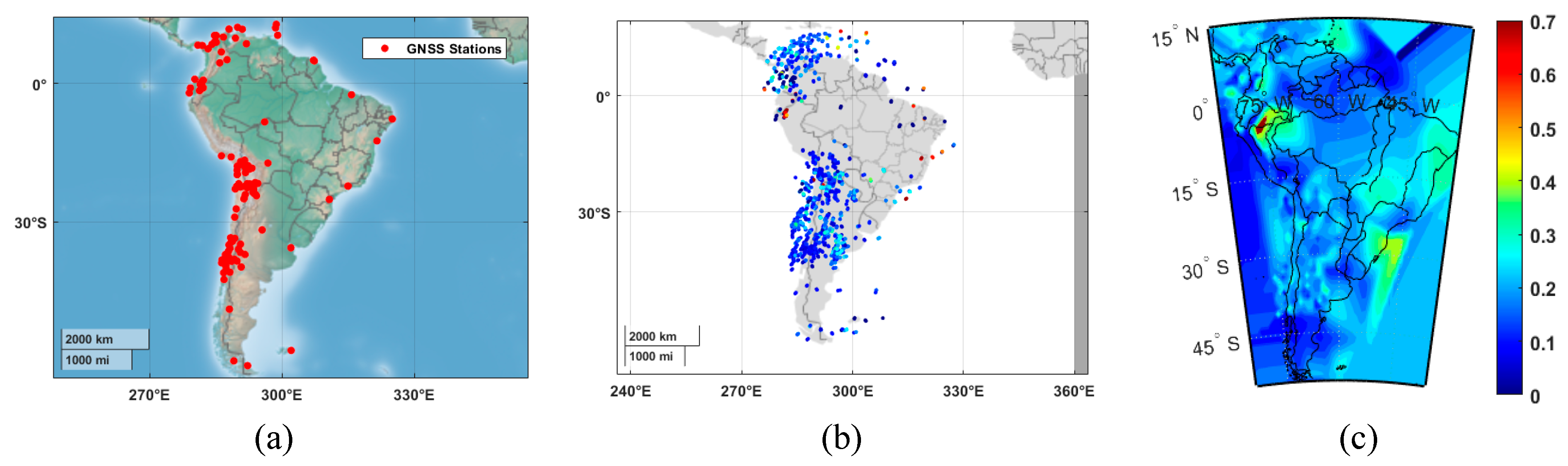
2. Data Collection
3. Methodology
3.1. Gated Recurrent Unit (GRU)
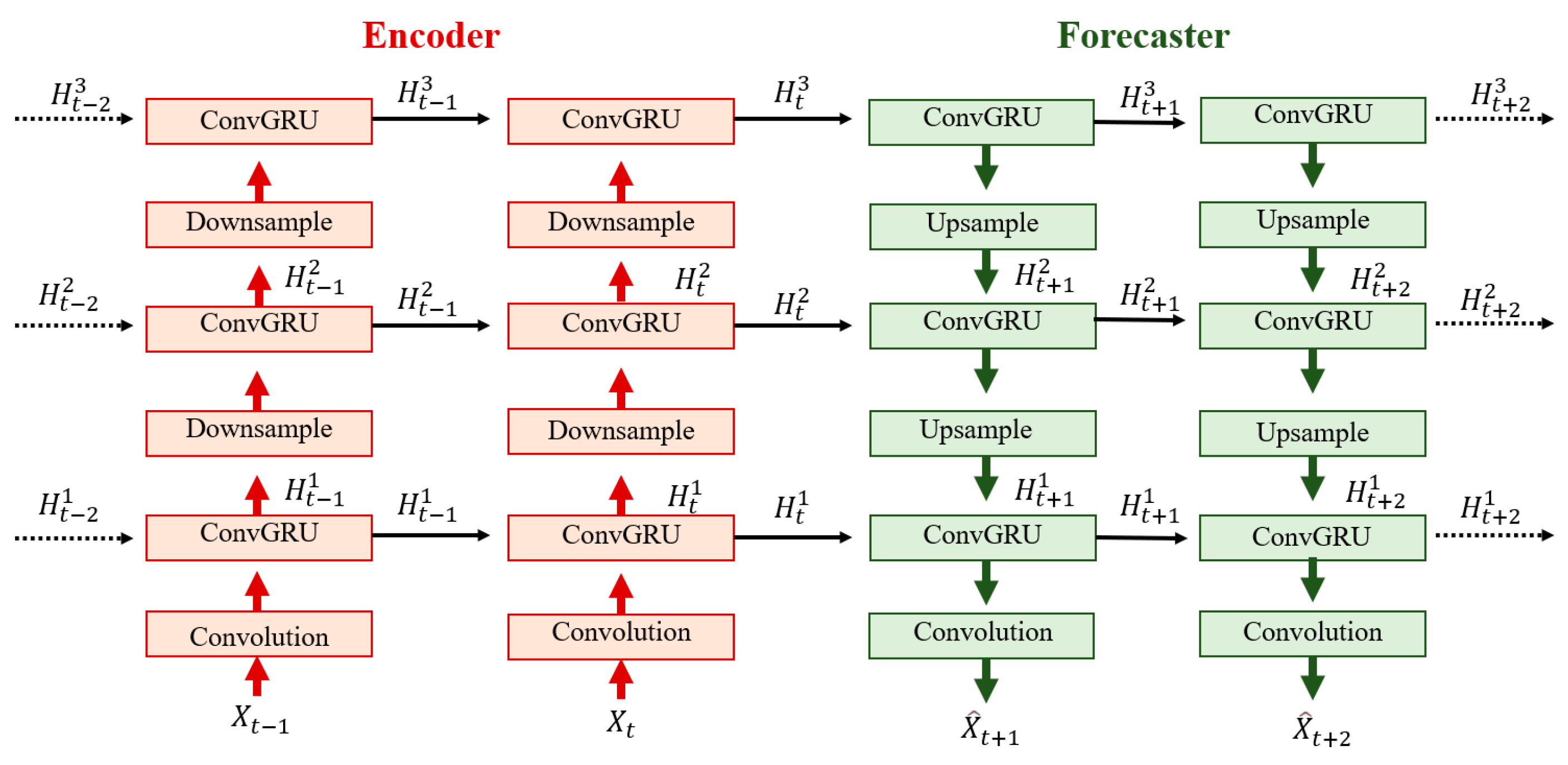
3.2. Convolutional Gated Recurrent Unit (ConvGRU)
3.3. Loss Function
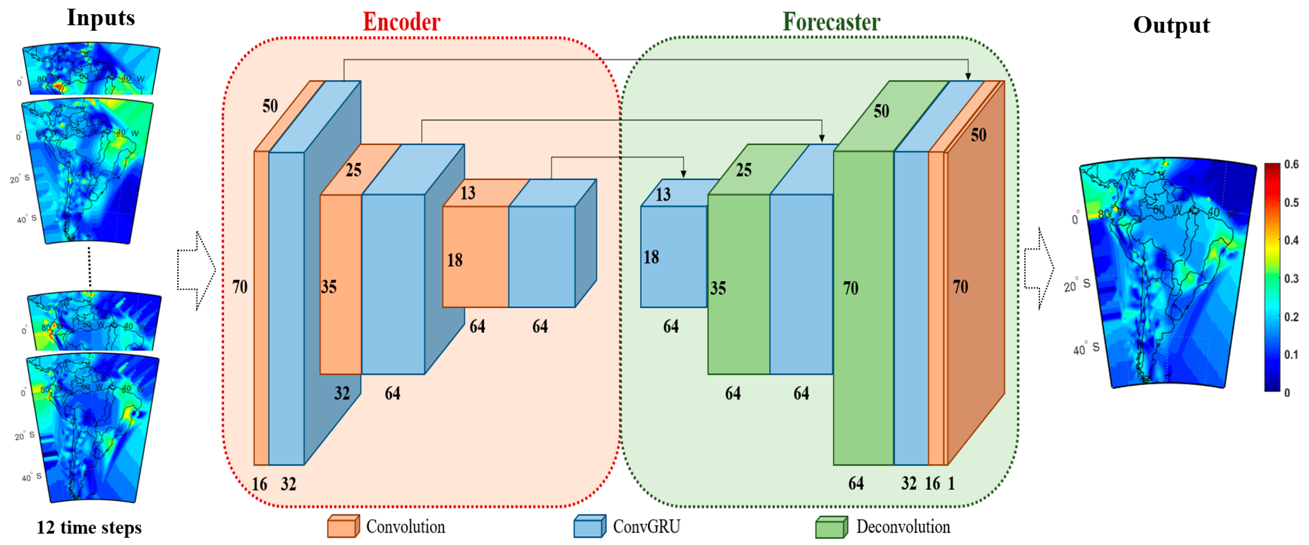
3.4. ConvGRU Algorithm Architecture
4. Geomagnetic Activities Affecting Ionospheric Scintillation
5. Results and Discussion
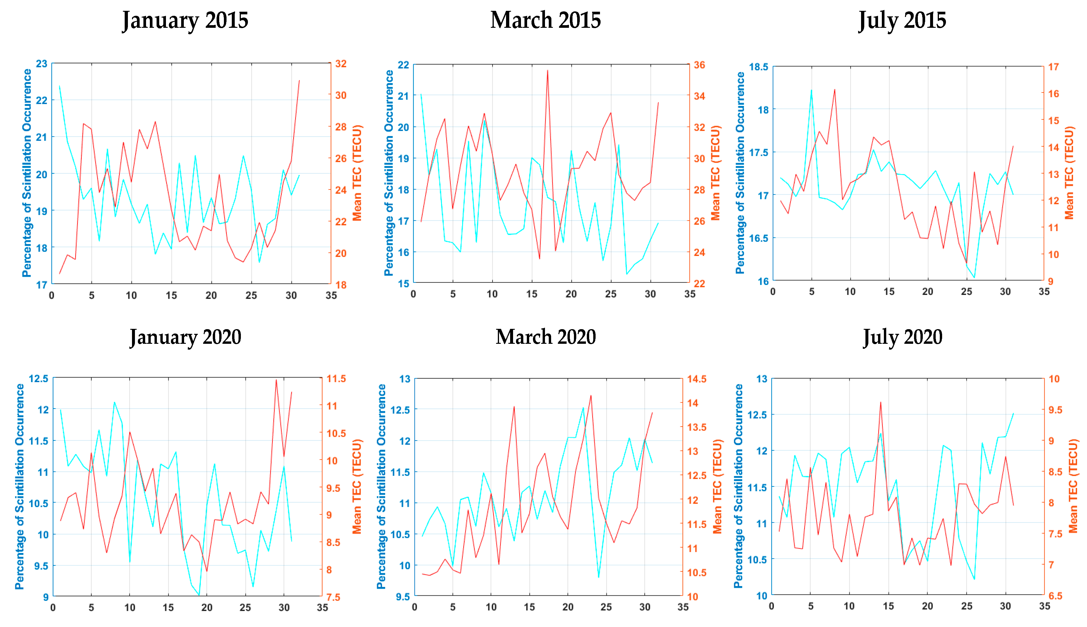
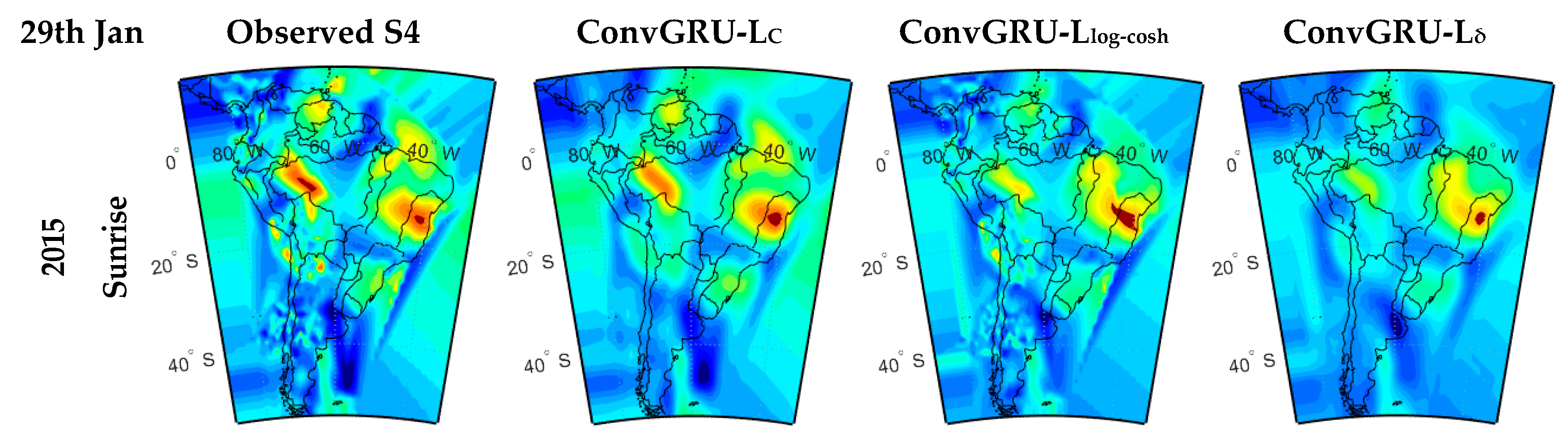
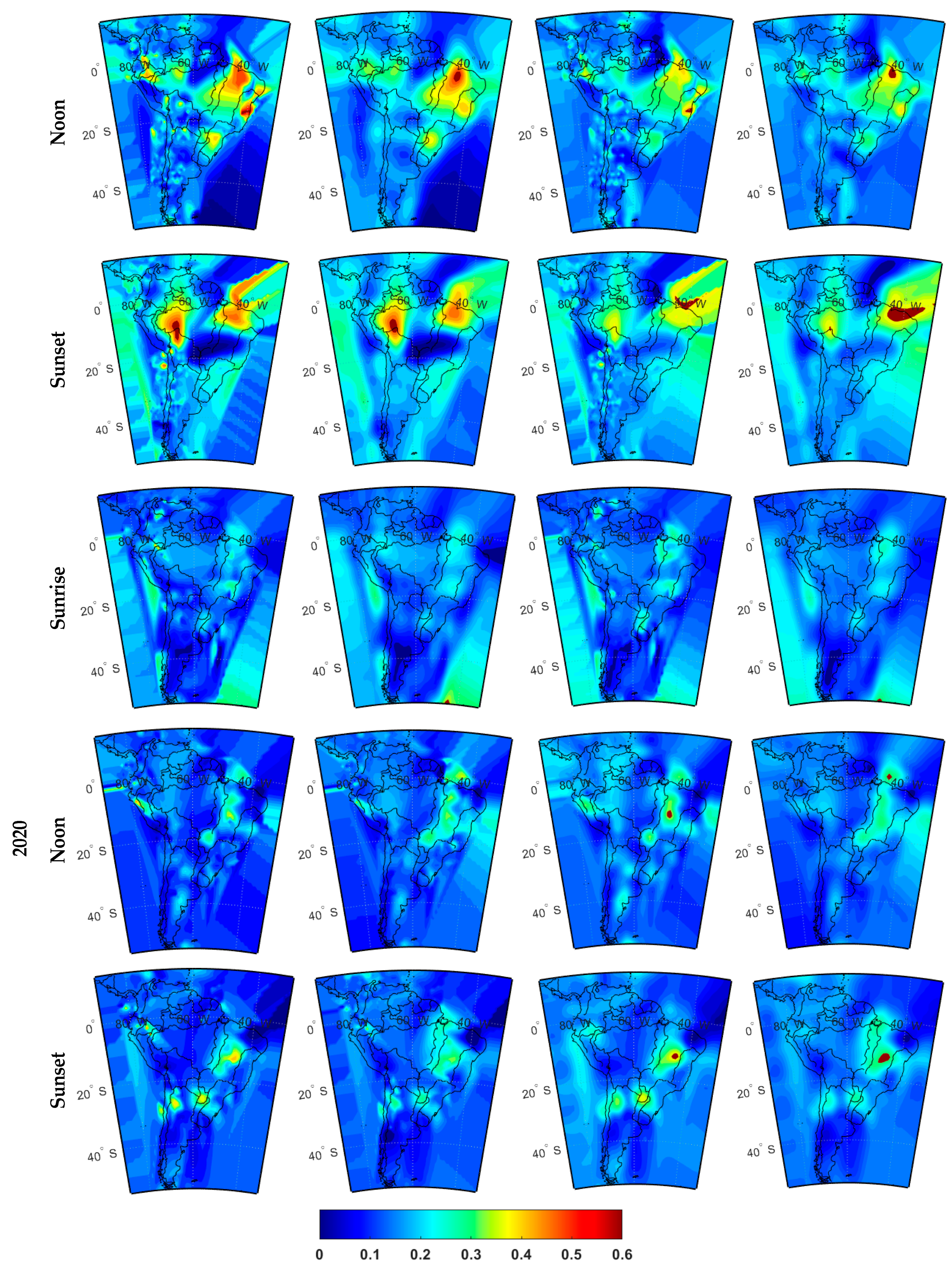
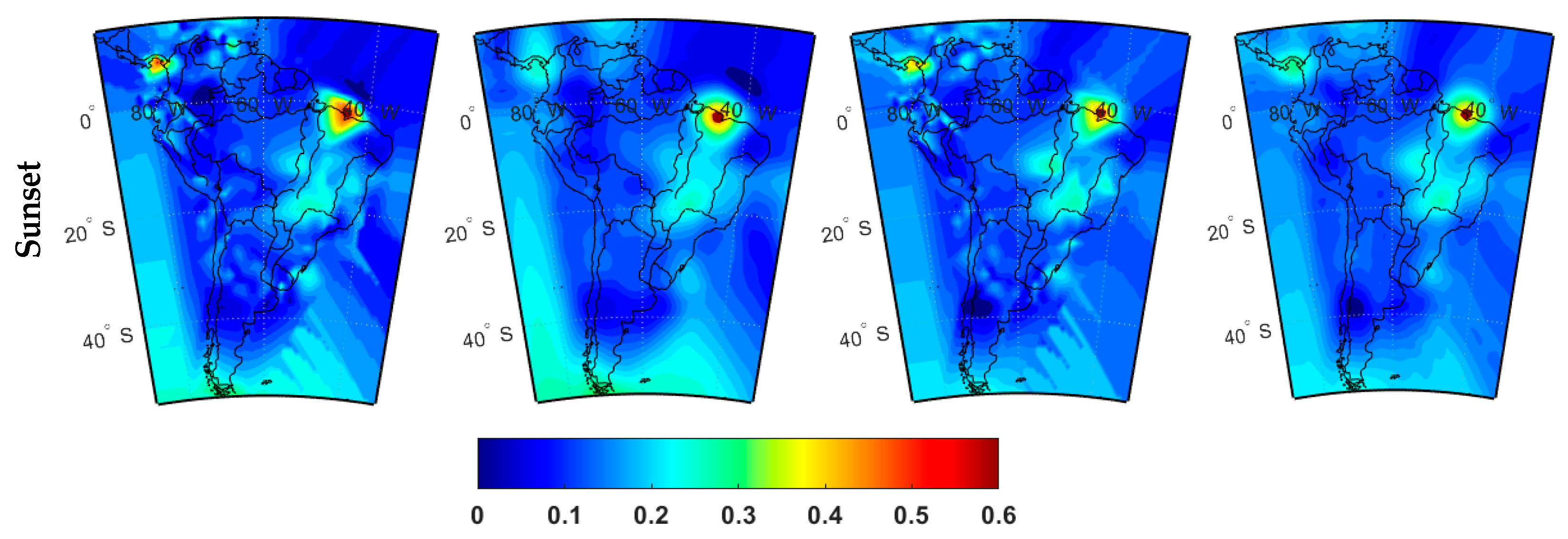
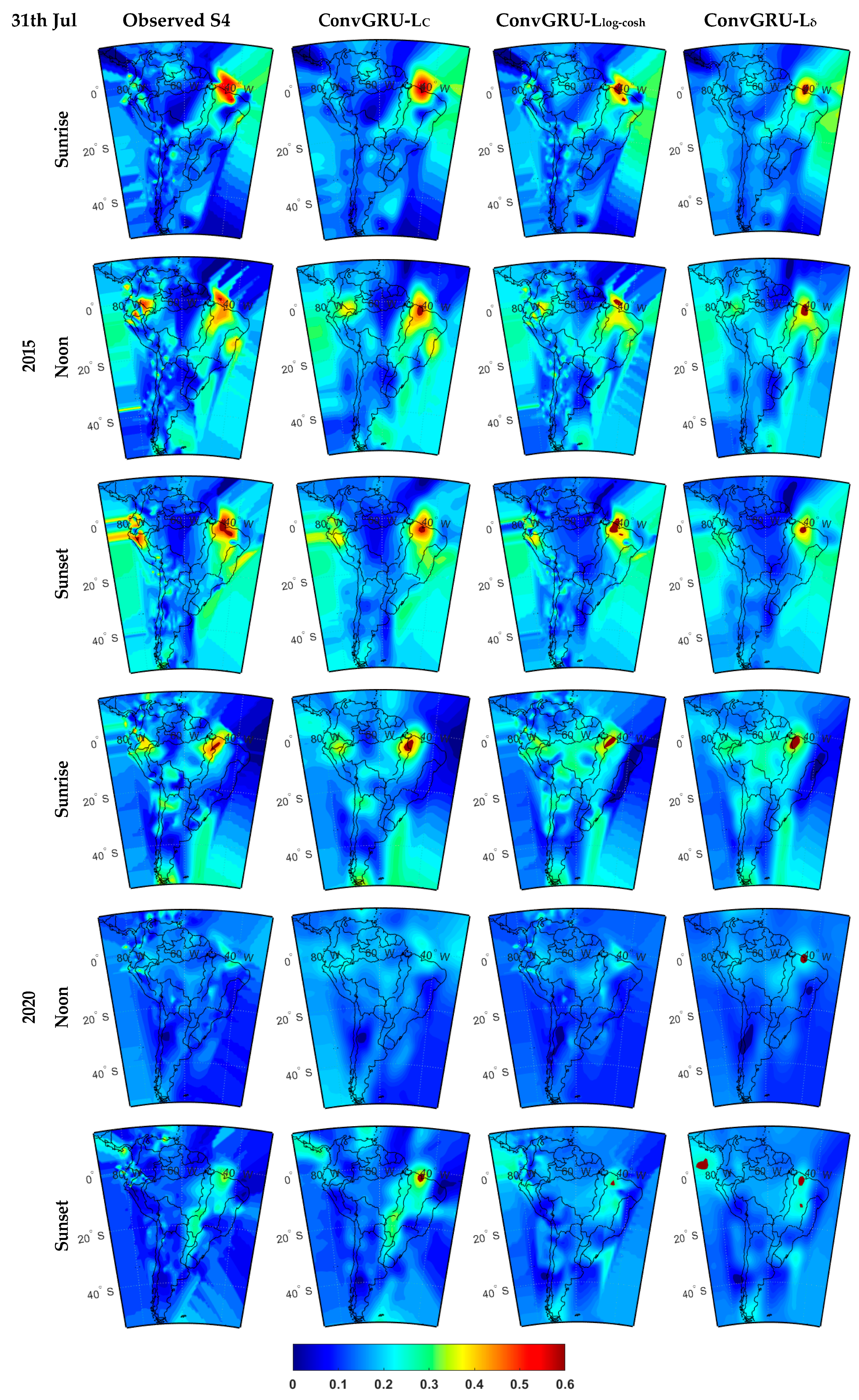
5.1. Comparative Analysis of Ionospheric Scintillations
5.2. Quantitative Analysis of the ConvGRU Models Efficacy
5.3. Comparative and Qualitative Analysis
6. Evaluation of Results
7. Conclusions
Author Contributions
Funding
Data Availability Statement
Conflicts of Interest
References
- Klobuchar, J.A. Ionospheric time-delay algorithm for single-frequency GPS users. IEEE Trans. Aerosp. Electron. Syst. 1987, 3, 325–331. [Google Scholar] [CrossRef]
- Prieto-Cerdeira, R.; Orús-Pérez, R.; Breeuwer, E.; Lucas-Rodriguez, R.; Falcone, M. Performance of the Galileo single-frequency ionospheric correction during in-orbit validation. GPS World 2014, 25, 53–58. [Google Scholar]
- Yuan, Y.; Wang, N.; Li, Z.; Huo, X. The BeiDou global broadcast ionospheric delay correction model (BDGIM) and its preliminary performance evaluation results. Navigation 2019, 66, 55–69. [Google Scholar] [CrossRef]
- Pi, X.; Mannucci, A.J.; Lindqwister, U.J.; Ho, C.M. Monitoring of global ionospheric irregularities using the worldwide GPS network. Geophys. Res. Lett. 1997, 24, 2283–2286. [Google Scholar] [CrossRef]
- Yang, Z.; Morton, Y.J.; Zakharenkova, I.; Cherniak, I.; Song, S.; Li, W. Global view of ionospheric disturbance impacts on kinematic GPS positioning solutions during the 2015 St. Patrick’s Day storm. J. Geophys. Res. Space Phys. 2020, 125, e2019JA027681. [Google Scholar] [CrossRef]
- Atabati, A.; Jazireeyan, I.; Alizadeh, M.; Pirooznia, M.; Flury, J.; Schuh, H.; Soja, B. Analyzing the Ionospheric Irregularities Caused by the September 2017 Geomagnetic Storm Using Ground-Based GNSS, Swarm, and FORMOSAT-3/COSMIC Data near the Equatorial Ionization Anomaly in East Africa. Remote Sens. 2023, 15, 5762. [Google Scholar] [CrossRef]
- Kelley, M.C. The Earth’s Ionosphere: Plasma Physics and Electrodynamics; Academic Press: Cambridge, MA, USA, 2009. [Google Scholar]
- Appleton, E.V. The anomalous equatorial belt in the F2-layer. J. Atmos. Terr. Phys. 1954, 5, 348–351. [Google Scholar] [CrossRef]
- Sultan, P.J. Linear theory and modeling of the Rayleigh-Taylor instability leading to the occurrence of equatorial spread F. J. Geophys. Res. Space Phys. 1996, 101, 26875–26891. [Google Scholar] [CrossRef]
- Li, G.; Ning, B.; Otsuka, Y.; Abdu, M.A.; Abadi, P.; Liu, Z.; Spogli, L.; Wan, W. Challenges to equatorial plasma bubble and ionospheric scintillation short-term forecasting and future aspects in east and southeast Asia. Surv. Geophys. 2021, 42, 201–238. [Google Scholar] [CrossRef]
- Fejer, B.G.; Scherliess, L.; De Paula, E.R. Effects of the vertical plasma drift velocity on the generation and evolution of equatorial spread F. J. Geophys. Res. Space Phys. 1999, 104, 19859–19869. [Google Scholar] [CrossRef]
- Aveiro, H.C.; Hysell, D.L. Three-dimensional numerical simulation of equatorial F region plasma irregularities with bottomside shear flow. J. Geophys. Res. Space Phys. 2010, 115. [Google Scholar] [CrossRef]
- Abdu, M.A.; Bittencourt, J.A.; Batista, I.S. Magnetic declination control of the equatorial F region dynamo electric field development and spread F. J. Geophys. Res. Space Phys. 1981, 86, 11443–11446. [Google Scholar] [CrossRef]
- Humphreys, T.E.; Psiaki, M.L.; Kintner, P.M. Modeling the effects of ionospheric scintillation on GPS carrier phase tracking. IEEE Trans. Aerosp. Electron. Syst. 2010, 46, 1624–1637. [Google Scholar] [CrossRef]
- Skone, S.; Lachapelle, G.; Yao, D.; Yu, W.; Watson, R. Investigating the impact of ionospheric scintillation using a GPS software receiver. In Proceedings of the 18th International Technical Meeting of the Satellite Division of The Institute of Navigation (ION GNSS 2005), Long Beach, CA, USA, 13–16 September 2005; pp. 1126–1137. [Google Scholar]
- Tiwari, R.; Strangeways, H.J.; Skone, S. Modeling the effects of ionospheric scintillation on GPS carrier phase tracking using high-rate TEC data. In Proceedings of the 26th International Technical Meeting of the Satellite Division of The Institute of Navigation (ION GNSS+ 2013), Nashville, TN, USA, 16–20 September 2013; pp. 2480–2488. [Google Scholar]
- Doherty, P.H.; Delay, S.H.; Valladares, C.E.; Klobuchar, J.A. Ionospheric scintillation effects on GPS in the equatorial and auroral regions. Navigation 2003, 50, 235–245. [Google Scholar] [CrossRef]
- Won, J.H.; Eissfeller, B.; Pany, T.; Winkel, J. Advanced signal processing scheme for GNSS receivers under ionospheric scintillation. In Proceedings of the 2012 IEEE/ION Position, Location and Navigation Symposium, Myrtle Beach, SC, USA, 23–26 April 2012; pp. 44–49. [Google Scholar]
- Sun, Y.; Zhang, H.; Hu, S.; Shi, J.; Geng, J.; Su, Y. ConvGRU-RMWP: A Regional Multi-Step Model for Wave Height Prediction. Mathematics 2023, 11, 2013. [Google Scholar] [CrossRef]
- Gu, C.; Li, H. Review on deep learning research and applications in wind and wave energy. Energies 2022, 15, 1510. [Google Scholar] [CrossRef]
- Simonyan, K.; Zisserman, A. Very deep convolutional networks for large-scale image recognition. arXiv 2014, arXiv:1409.1556. [Google Scholar]
- Pouyanfar, S.; Sadiq, S.; Yan, Y.; Tian, H.; Tao, Y.; Reyes, M.P.; Shyu, M.L.; Chen, S.C.; Iyengar, S.S. A survey on deep learning: Algorithms, techniques, and applications. ACM Comput. Surv. (CSUR) 2018, 51, 1–36. [Google Scholar] [CrossRef]
- Kalchbrenner, N.; Grefenstette, E.; Blunsom, P. A convolutional neural network for modelling sentences. arXiv 2014, arXiv:1404.2188. [Google Scholar]
- Mandic, D.P.; Chambers, J. Recurrent Neural Networks for Prediction: Learning Algorithms, Architectures and Stability; John Wiley & Sons, Inc.: Hoboken, NJ, USA, 2001. [Google Scholar]
- Hochreiter, S.; Schmidhuber, J. Long short-term memory. Neural Comput. 1997, 9, 1735–1780. [Google Scholar] [CrossRef]
- Dey, R.; Salem, F.M. Gate-variants of gated recurrent unit (GRU) neural networks. In Proceedings of the 2017 IEEE 60th International Midwest Symposium on Circuits and Systems (MWSCAS), Boston, MA, USA, 6–9 August 2017; pp. 1597–1600. [Google Scholar]
- Das, A.; Gupta, A.D.; Ray, S. Characteristics of L-band (1.5 GHz) and VHF (244 MHz) amplitude scintillations recorded at Kolkata during 1996–2006 and development of models for the occurrence probability of scintillations using neural network. J. Atmos. Sol. Terr. Phys. 2010, 72, 685–704. [Google Scholar] [CrossRef]
- Rezende, L.F.C.D.; De Paula, E.R.; Stephany, S.; Kantor, I.J.; Muella, M.T.A.H.; De Siqueira, P.M.; Correa, K.S. Survey and prediction of the ionospheric scintillation using data mining techniques. Space Weather 2010, 8. [Google Scholar] [CrossRef]
- Prikryl, P.; Jayachandran, P.T.; Mushini, S.C.; Richardson, I.G. Toward the probabilistic forecasting of high-latitude GPS phase scintillation. Space Weather 2012, 10. [Google Scholar] [CrossRef]
- De Lima, G.R.T.; Stephany, S.; De Paula, E.R.; Batista, I.S.; Abdu, M.A. Prediction of the level of ionospheric scintillation at equatorial latitudes in Brazil using a neural network. Space Weather 2015, 13, 446–457. [Google Scholar] [CrossRef]
- Atabati, A.; Alizadeh, M.; Schuh, H.; Tsai, L.C. Ionospheric scintillation prediction on s4 and roti parameters using artificial neural network and genetic algorithm. Remote Sens. 2021, 13, 2092. [Google Scholar] [CrossRef]
- McGranaghan, R.M.; Mannucci, A.J.; Wilson, B.; Mattmann, C.A.; Chadwick, R. New capabilities for prediction of high-latitude ionospheric scintillation: A novel approach with machine learning. Space Weather 2018, 16, 1817–1846. [Google Scholar] [CrossRef]
- Ruwali, A.; Kumar, A.S.; Prakash, K.B.; Sivavaraprasad, G.; Ratnam, D.V. Implementation of hybrid deep learning model (LSTM-CNN) for ionospheric TEC forecasting using GPS data. IEEE Geosci. Remote Sens. Lett. 2020, 18, 1004–1008. [Google Scholar] [CrossRef]
- Sun, W.; Xu, L.; Huang, X.; Zhang, W.; Yuan, T.; Chen, Z.; Yan, Y. Forecasting of ionospheric vertical total electron content (TEC) using LSTM networks. In Proceedings of the 2017 International Conference on Machine Learning and Cybernetics (ICMLC), Ningbo, China, 9–12 July 2017; Volume 2, pp. 340–344. [Google Scholar]
- Liu, L.; Morton, Y.J.; Liu, Y. Machine Learning Prediction of Storm-Time High-Latitude Ionospheric Irregularities from GNSS-Derived ROTI Maps. Geophys. Res. Lett. 2021, 48, e2021GL095561. [Google Scholar] [CrossRef]
- Shi, X.; Chen, Z.; Wang, H.; Yeung, D.Y.; Wong, W.K.; Woo, W.C. Convolutional LSTM network: A machine learning approach for precipitation nowcasting. Adv. Neural Inf. Process. Syst. 2015, 28, 802–810. [Google Scholar]
- Shi, X.; Gao, Z.; Lausen, L.; Wang, H.; Yeung, D.Y.; Wong, W.K.; Woo, W.C. Deep learning for precipitation nowcasting: A benchmark and a new model. Adv. Neural Inf. Process. Syst. 2017, 30, 5622–5632. [Google Scholar]
- Liu, L.; Yao, Y.; Aa, E. Multi-instrumental observations of early morning equatorial plasma depletions during the 2017 memorial weekend storm. IEEE J. Sel. Top. Appl. Earth Obs. Remote Sens. 2020, 13, 5351–5357. [Google Scholar] [CrossRef]
- Hong, C.K.; Grejner-Brzezinska, D.A.; Kwon, J.H. Efficient GPS receiver DCB estimation for ionosphere modeling using satellite-receiver geometry changes. Earth Planets Space 2008, 60, e25–e28. [Google Scholar] [CrossRef]
- Arikan, F.E.Z.A.; Erol, C.B.; Arikan, O. Regularized estimation of vertical total electron content from GPS data for a desired time period. Radio Sci. 2004, 39, 1–10. [Google Scholar] [CrossRef]
- Van Dierendonck, A.J.; Klobuchar, J.; Hua, Q. Ionospheric scintillation monitoring using commercial single frequency C/A code receivers. In Proceedings of the ION GPS, Salt Lake City, UT, USA, 22–24 September 1993; Volume 93, pp. 1333–1342. [Google Scholar]
- Juan, J.M.; Aragon-Angel, A.; Sanz, J.; González-Casado, G.; Rovira-Garcia, A. A method for scintillation characterization using geodetic receivers operating at 1 Hz. J. Geod. 2017, 91, 1383–1397. [Google Scholar] [CrossRef]
- Tiwari, R.; Strangeways, H.J. Regionally based alarm index to mitigate ionospheric scintillation effects for GNSS receivers. Space Weather 2015, 13, 72–85. [Google Scholar] [CrossRef]
- Van Dierendonck, A.J.; Arbesser-Rastburg, B. Measuring ionospheric scintillation in the equatorial region over Africa, including measurements from SBAS geostationary satellite signals. In Proceedings of the 17th International Technical Meeting of the Satellite Division of The Institute of Navigation (ION GNSS 2004), Long Beach, CA, USA, 21–24 September 2004; pp. 316–324. [Google Scholar]
- Alfonsi, L.; Spogli, L.; Tong, J.R.; De Franceschi, G.; Romano, V.; Bourdillon, A.; Le Huy, M.; Mitchell, C.N. GPS scintillation and TEC gradients at equatorial latitudes in April 2006. Adv. Space Res. 2011, 47, 1750–1757. [Google Scholar] [CrossRef]
- Xiong, B.; Wan, W.X.; Ning, B.Q.; Yuan, H.; Li, G.Z. A comparison and analysis of the S4 index, C/N and Roti over Sanya. Chin. J. Geophys. 2007, 50, 1414–1424. [Google Scholar]
- Carbonell, J.G.; Michalski, R.S.; Mitchell, T.M. An overview of machine learning. Mach. Learn. 1983, 3–23. [Google Scholar] [CrossRef]
- Haykin, S. Neural Networks and Learning Machines, 3/E; Pearson Education: Karnataka, India, 2009. [Google Scholar]
- Norgaard, M. Neural Network-Based System Identification Toolbox; Department of Automation, Technical University of Denmark: Kongens Lyngby, Denmark, 2000. [Google Scholar]
- Zhang, D.; Kabuka, M.R. Combining weather condition data to predict traffic flow: A GRU-based deep learning approach. IET Intell. Transp. Syst. 2018, 12, 578–585. [Google Scholar] [CrossRef]
- Dai, G.; Ma, C.; Xu, X. Short-term traffic flow prediction method for urban road sections based on space–time analysis and GRU. IEEE Access 2019, 7, 143025–143035. [Google Scholar] [CrossRef]
- Maas, A.L.; Hannun, A.Y.; Ng, A.Y. Rectifier nonlinearities improve neural network acoustic models. In Proceedings of the ICML, Atlanta, GA, USA, 16–21 June 2013; Volume 30, No. 1. p. 3. [Google Scholar]
- Liu, X.; Lin, Z.; Feng, Z. Short-term offshore wind speed forecast by seasonal ARIMA-A comparison against GRU and LSTM. Energy 2021, 227, 120492. [Google Scholar] [CrossRef]
- Martin-Donas, J.M.; Gomez, A.M.; Gonzalez, J.A.; Peinado, A.M. A deep learning loss function based on the perceptual evaluation of the speech quality. IEEE Signal Process. Lett. 2018, 25, 1680–1684. [Google Scholar] [CrossRef]
- Qi, J.; Du, J.; Siniscalchi, S.M.; Ma, X.; Lee, C.H. On mean absolute error for deep neural network-based vector-to-vector regression. IEEE Signal Process. Lett. 2020, 27, 1485–1489. [Google Scholar] [CrossRef]
- Barron, J.T. A general and adaptive robust loss function. In Proceedings of the IEEE/CVF Conference on Computer Vision and Pattern Recognition, Long Beach, CA, USA, 15–20 June 2019; pp. 4331–4339. [Google Scholar]
- Wang, Q.; Ma, Y.; Zhao, K.; Tian, Y. A comprehensive survey of loss functions in machine learning. Ann. Data Sci. 2020, 9, 187–212. [Google Scholar] [CrossRef]
- Li, G.; Ning, B.; Zhao, B.; Liu, L.; Liu, J.Y.; Yumoto, K. Effects of geomagnetic storm on GPS ionospheric scintillations at Sanya. J. Atmos. Sol.-Terr. Phys. 2008, 70, 1034–1045. [Google Scholar] [CrossRef]
- Li, G.; Ning, B.; Wang, C.; Abdu, M.A.; Otsuka, Y.; Yamamoto, M.; Wu, J.; Chen, J. Storm-enhanced development of postsunset equatorial plasma bubbles around the meridian 120°E/60°W on 7–8 September 2017. J. Geophys. Res. Space Phys. 2018, 123, 7985–7998. [Google Scholar] [CrossRef]
- Zolesi, B.; Cander, L.R. Ionospheric Prediction and Forecasting; Springer: Berlin/Heidelberg, Germany, 2014. [Google Scholar]
- De Lima, G.R.T.; Stephany, S.; De Paula, E.R.; Batista, I.S.; Abdu, M.A.; Rezende, L.F.C.D.; Aquino, M.G.D.S.; Dutra, A.P.S. Correlation analysis between the occurrence of ionospheric scintillation at the magnetic equator and at the southern peak of the Equatorial Ionization Anomaly. Space Weather 2014, 12, 406–416. [Google Scholar] [CrossRef]
- de Paula, E.R.; de Oliveira, C.B.; Caton, R.G.; Negreti, P.M.; Batista, I.S.; Martinon, A.R.; Neto, A.C.; Abdu, M.A.; Monico, J.F.; Sousasantos, J.; et al. Ionospheric irregularity behavior during the September 6–10, 2017 magnetic storm over Brazilian equatorial–low latitudes. Earth Planets Space 2019, 71, 42. [Google Scholar] [CrossRef]
- Kaselimi, M.; Voulodimos, A.; Doulamis, N.; Doulamis, A.; Delikaraoglou, D. Deep recurrent neural networks for ionospheric variations estimation using GNSS measurements. IEEE Trans. Geosci. Remote Sens. 2021, 60, 5800715. [Google Scholar] [CrossRef]
- Kingma, D.P.; Ba, J. Adam: A method for stochastic optimization. arXiv 2014, arXiv:1412.6980. [Google Scholar]
- Xu, B.; Wang, N.; Chen, T.; Li, M. Empirical evaluation of rectified activations in convolutional network. arXiv 2015, arXiv:1505.00853. [Google Scholar]
- Goodfellow, I.; Bengio, Y.; Courville, A. Deep Learning; MIT Press: Cambridge, MA, USA, 2016. [Google Scholar]
- Allouche, O.; Tsoar, A.; Kadmon, R. Assessing the accuracy of species distribution models: Prevalence, kappa and the true skill statistic (TSS). J. Appl. Ecol. 2006, 43, 1223–1232. [Google Scholar] [CrossRef]
- Fowle, M.A.; Roebber, P.J. Short-range (0–48 h) numerical prediction of convective occurrence, mode, and location. Weather Forecast. 2003, 18, 782–794. [Google Scholar] [CrossRef]
- Schaefer, J.T. The critical success index as an indicator of warning skill. Weather Forecast. 1990, 5, 570–575. [Google Scholar] [CrossRef]
- Wehling, P.; LaBudde, R.A.; Brunelle, S.L.; Nelson, M.T. Probability of detection (POD) as a statistical model for the validation of qualitative methods. J. AOAC Int. 2011, 94, 335–347. [Google Scholar] [CrossRef]


| Period of Time | Dst (nT) | Kp | Sunspot Number (SSN) | Solar Flux F10.7 | |||||
|---|---|---|---|---|---|---|---|---|---|
| Mean | Max | Mean | Max | Mean | Max | Mean | Max | ||
| 2015 | January | −20.56 | 36 | 1.96 | 6.33 | 93.65 | 153 | 137.32 | 171.80 |
| March | −27.75 | 45 | 2.46 | 7.66 | 54.18 | 108 | 126.29 | 145.60 | |
| July | −19.43 | 28 | 1.71 | 5.66 | 65.78 | 123 | 106.91 | 133.40 | |
| 2020 | January | −3.63 | 21 | 1.02 | 3.66 | 6.18 | 19 | 72.23 | 74.70 |
| March | −5.76 | 12 | 1.34 | 4.33 | 1.84 | 16 | 70.12 | 72.10 | |
| July | −4.73 | 22 | 0.96 | 4 | 6.68 | 26 | 69.57 | 73.30 | |
| Period of Time | 2015 | 2020 | ||||||
|---|---|---|---|---|---|---|---|---|
| January | March | July | January | March | July | |||
| Ionospheric conditions | Mean VTEC (TECU) | 23.31 | 29.26 | 12.36 | 9.26 | 11.81 | 7.77 | |
| Mean S4 | 0.152 | 0.148 | 0.147 | 0.130 | 0.128 | 0.130 | ||
| Scintillation Occurrence (S4 > 0.2) | 19.32% | 17.46% | 17.09% | 10.55% | 11.14% | 11.50% | ||
| ConvGRU-LC | Modeling | CC | 0.91 | 0.91 | 0.92 | 0.94 | 0.92 | 0.92 |
| RMSE | 0.008 | 0.009 | 0.009 | 0.006 | 0.007 | 0.007 | ||
| Mean Error (ME) | 0.019 | 0.017 | 0.016 | 0.011 | 0.013 | 0.014 | ||
| Prediction | CC | 0.80 | 0.80 | 0.81 | 0.83 | 0.82 | 0.85 | |
| RMSE | 0.024 | 0.024 | 0.022 | 0.013 | 0.016 | 0.016 | ||
| Mean Error (ME) | 0.04 | 0.04 | 0.03 | 0.02 | 0.02 | 0.02 | ||
| ConvGRU-Llog-cosh | Modeling | CC | 0.88 | 0.89 | 0.89 | 0.91 | 0.90 | 0.90 |
| RMSE | 0.013 | 0.013 | 0.012 | 0.010 | 0.010 | 0.011 | ||
| Mean Error (ME) | 0.025 | 0.023 | 0.022 | 0.019 | 0.020 | 0.021 | ||
| Prediction | CC | 0.77 | 0.78 | 0.78 | 0.81 | 0.80 | 0.83 | |
| RMSE | 0.039 | 0.035 | 0.030 | 0.022 | 0.023 | 0.025 | ||
| Mean Error (ME) | 0.06 | 0.05 | 0.04 | 0.03 | 0.03 | 0.03 | ||
| ConvGRU-Lδ | Modeling | CC | 0.86 | 0.86 | 0.87 | 0.92 | 0.91 | 0.90 |
| RMSE | 0.014 | 0.014 | 0.013 | 0.009 | 0.010 | 0.010 | ||
| Mean Error (ME) | 0.026 | 0.025 | 0.024 | 0.018 | 0.019 | 0.021 | ||
| Prediction | CC | 0.75 | 0.75 | 0.76 | 0.80 | 0.79 | 0.81 | |
| RMSE | 0.042 | 0.038 | 0.032 | 0.020 | 0.019 | 0.023 | ||
| Mean Error (ME) | 0.07 | 0.06 | 0.05 | 0.04 | 0.04 | 004 | ||
| Period of Time | 2015 | 2020 | |||||
|---|---|---|---|---|---|---|---|
| January | March | July | January | March | July | ||
| ConvGRU-LC | FAR | 0.34 | 0.32 | 0.28 | 0.19 | 0.21 | 0.16 |
| CSI | 0.43 | 0.45 | 0.52 | 0.64 | 0.66 | 0.70 | |
| POD | 0.59 | 0.61 | 0.65 | 0.80 | 0.81 | 0.83 | |
| TSS | 0.53 | 0.55 | 0.58 | 0.72 | 0.73 | 0.76 | |
| ConvGRU-Llog-cosh | FAR | 0.36 | 0.34 | 0.30 | 0.20 | 0.22 | 0.17 |
| CSI | 0.41 | 0.44 | 0.50 | 0.62 | 0.64 | 0.68 | |
| POD | 0.56 | 0.59 | 0.62 | 0.78 | 0.79 | 0.81 | |
| TSS | 0.51 | 0.53 | 0.55 | 0.70 | 0.71 | 0.74 | |
| ConvGRU-Lδ | FAR | 0.37 | 0.35 | 0.32 | 0.21 | 0.23 | 0.18 |
| CSI | 0.40 | 0.42 | 0.47 | 0.61 | 0.63 | 0.66 | |
| POD | 0.55 | 0.57 | 0.58 | 0.76 | 0.77 | 0.79 | |
| TSS | 0.49 | 0.51 | 0.54 | 0.69 | 0.70 | 0.72 | |
Disclaimer/Publisher’s Note: The statements, opinions and data contained in all publications are solely those of the individual author(s) and contributor(s) and not of MDPI and/or the editor(s). MDPI and/or the editor(s) disclaim responsibility for any injury to people or property resulting from any ideas, methods, instructions or products referred to in the content. |
© 2024 by the authors. Licensee MDPI, Basel, Switzerland. This article is an open access article distributed under the terms and conditions of the Creative Commons Attribution (CC BY) license (https://creativecommons.org/licenses/by/4.0/).
Share and Cite
Atabati, A.; Jazireeyan, I.; Alizadeh, M.; Langley, R.B. Prediction of Ionospheric Scintillation with ConvGRU Networks Using GNSS Ground-Based Data across South America. Remote Sens. 2024, 16, 2757. https://doi.org/10.3390/rs16152757
Atabati A, Jazireeyan I, Alizadeh M, Langley RB. Prediction of Ionospheric Scintillation with ConvGRU Networks Using GNSS Ground-Based Data across South America. Remote Sensing. 2024; 16(15):2757. https://doi.org/10.3390/rs16152757
Chicago/Turabian StyleAtabati, Alireza, Iraj Jazireeyan, Mahdi Alizadeh, and Richard B. Langley. 2024. "Prediction of Ionospheric Scintillation with ConvGRU Networks Using GNSS Ground-Based Data across South America" Remote Sensing 16, no. 15: 2757. https://doi.org/10.3390/rs16152757