Abstract
Synthetic aperture radar (SAR) technology has become an important means of flood monitoring because of its large coverage, repeated observation, and all-weather and all-time working capabilities. The commonly used thresholding and change detection methods in emergency monitoring can quickly and simply detect floods. However, these methods still have some problems: (1) thresholding methods are easily affected by low backscattering regions and speckle noise; (2) changes from multi-temporal information include urban renewal and seasonal variation, reducing the precision of flood monitoring. To solve these problems, this paper presents a new flood mapping framework that combines semi-automatic thresholding and change detection. First, multiple lines across land and water are drawn manually, and their local optimal thresholds are calculated automatically along these lines from two ends towards the middle. Using the average of these thresholds, the low backscattering regions are extracted to generate a preliminary inundation map. Then, the neighborhood-based change detection method combined with entropy thresholding is adopted to detect the changed areas. Finally, pixels in both the low backscattering regions and the changed regions are marked as inundated terrain. Two flood datasets, one from Sentinel-1 in the Wharfe and Ouse River basin and another from GF-3 in Chaohu are chosen to verify the effectiveness and practicality of the proposed method.
1. Introduction
Flood disasters have the characteristics of wide coverage and strong suddenness, especially during wet seasons or rainy weather [1]. Affected by natural and human factors, floods have been one of the most frequent natural disasters in the past two decades [2]. Although the average number of deaths per flood disaster has decreased with the development of technology, the number of floods is increasing every year, which poses a great threat to human safety and property. How to accurately monitor the flood lifecycle has become an important part of emergency disaster management and rescue guidance [2,3].
As core tasks in flood mapping, the accurate extraction of water body data and the detection of water changes have been long-standing research hotspots [4,5]. The traditional methods obtain the water body information using manual field investigation or hydrological monitoring stations. Although these methods can achieve high accuracy, they can only perform point measurements with small coverage and require a significant amount of manpower and resources. In flood emergency monitoring, the on-site investigation method is usually difficult to rapidly apply in the affected area, while the monitoring stations method has difficulty reflecting the overall situation, making traditional methods inadequate in flood monitoring.
Thanks to the continuous development of satellite sensors, Earth observations from multi-source satellites provide the possibility of near real-time flood monitoring and more effectively support emergency management than gauged data [6]. As advanced earth observation means, both active and passive satellite remote sensing data can be widely used for inundation mapping at different stages of flood occurrence [7,8,9]. Due to the advantages of visualization and the interpretability of images, optical sensors can be used to obtain water surface data straightforwardly and reliably. With the accumulation of long-term and high-resolution satellite data, many optical remote sensing approaches contribute significantly to the delineation of global and regional water surfaces [10,11]. As flooding is often accompanied by extreme weather, passive optical sensors are frequently affected by clouds and unclear weather conditions, resulting in reduced effectiveness during flood events. Alternatively, active microwave sensors, especially the synthetic aperture radar (SAR), provide their own illumination of the Earth’s surface and thus can observe day and night, as well as through cloud cover [12], which is very suitable for monitoring during and after flood events [13,14,15]. SAR remote sensing technology is suitable for information extraction of the flood lifecycle because of its advantages in large-scale, all-weather, and all-day and -night monitoring.
Considering the characteristics of water bodies in SAR imagery, the radar backscatter of open calm water bodies is usually lower than the surrounding terrain, which makes it possible to detect floodwater in SAR imagery [6,16]. In general, the interaction between electromagnetic waves and calm water surfaces is mainly manifested as odd scattering, which makes the region of water dark in radar imagery. Moreover, the physical scattering of water bodies in SAR imagery is significantly different from land areas, which can be distinguished by several different kinds of approaches [17,18]. Among these methods, the thresholding method [19,20] is the most commonly used approach. Its application for water extraction is rather straightforward: a global threshold is applied to the whole scene, allowing the water to be separated from other land covers. The threshold can be selected by visual inspection of the backscatter histogram or by using automatic approaches [21]. Accurately selecting thresholds is vital to improve the accuracy of the flood mapping. Numerous automatic threshold selection methods have been developed [22,23,24], among which the Kittler and Illingworth’s minimum error thresholding (K&I) [25] method and Otsu’s maximum between-class variance [26] method are widely employed because of their simplicity and generalization. The K&I algorithm is based on Bayesian theory, and it determines the optimal threshold by minimizing the classification error. The Otsu algorithm calculates the between-class variance of the grayscale values for every possible threshold and determines the optimal threshold by maximizing the between-class variance.
Thresholding-based methods have the advantages of simple calculation and less time consumption while yielding competitive accuracy [27,28]. However, some other objects with low backscattering, such as farmlands, roads, and airstrips, are prone to interfere with the water extraction results, leading to over-detection in flood mapping. This phenomenon is caused by the same backscattering characteristics of different objects, which is difficult to overcome by a single temporal SAR image. By utilizing temporal information and comparing images from different periods, stable targets such as roads and shadows can be effectively removed [29]. Furthermore, floodwater can be distinguished from permanent water bodies by analyzing the decrease of backscattering caused by flooding-related compared to non-flood reference images [13,30]. Therefore, the change detection technique using multi-temporal information can map the flood by detecting the changes in floods.
Based on whether using a priori knowledge or sample information, the change detection approaches involve supervised and unsupervised approaches [31,32,33]. With the development of artificial intelligence technology, supervised change detection methods based on machine learning and deep learning technologies [32,33,34,35] are widely used. However, these methods need massive and high-quality samples, which are not suitable for rapid flood mapping of emergency responses. On the other hand, the unsupervised change detection methods are simple and efficient and can detect the flood regions without a priori knowledge or samples [34,35,36]. Considering the emergency needs of flood mapping, the unsupervised change detection methods are chosen in the proposed framework.
In general, unsupervised change detection involves several steps, including data preprocessing, the generation of difference images, and the extraction of changed regions. In the step of data preprocessing, multi-temporal SAR data are processed by radiometric calibration, co-registration, and speckle filtering. After obtaining accurate preprocessing results, many methods for difference image generation were designed for different polarizations, such as log-ratio [37,38], neighborhood-based ratio [39], and feature fusion [8,9] for single/dual polarization SAR data, as well as test statistic [23] and Hotelling–Lawley trace statistic [40] for fully polarized SAR data. Despite preprocessing, such as filtering, some noise may still exist in the difference image. In this situation, image segmentation methods [41,42,43] can be used to further suppress the impact of speckle noise. This type of method divides the image into multiple homogeneous regions, thereby reducing the false alarm rate of detection and improving the processing speed. In the step of changed region extraction, a number of methods have been developed for accurate and efficient automatic threshold selection, such as the K&I algorithm [25], Otsu [26], entropy thresholding [44], et al.
In order to overcome the limitations of using a single image and a single algorithm, more complex frameworks that integrate multi-image and multi-algorithm methods have been proposed [45] to achieve higher accuracy in flood mapping. Although these algorithms work well, few of them have been widely used in practice. On the one hand, some algorithms are relatively complex and rely on ground auxiliary data, making them difficult to understand and implement. On the other hand, some algorithms have low execution efficiency and can only obtain the ideal result by adjusting the parameters multiple times through the trial-and-error method. In this paper, we focus on the design of the flood mapping algorithm with the following characteristics: (1) accurate—both the false alarm rate and missing alarm rate are low, and the boundary between water and land is as accurate as possible; (2) efficient—the final result can be achieved as quickly as possible without the need for multiple trials and errors; (3) simple—both the principle and workflow are as simple as possible in order to facilitate implementation and operation by users.
Based on the above principles, we propose a rapid flood mapping framework to deal with sudden flood disasters in a short time. The main innovation is reflected in three aspects: First, a semi-automatic thresholding algorithm for preliminary flood extraction is proposed, which does not require parameter setting and multiple iterations. Second, a change detection algorithm considering neighborhood information is proposed to extract inundation areas while excluding permanent water bodies, which can effectively suppress the speckle noise. Third, the final flood map is extracted by combining the preliminary inundation map and the change map through a simple intersection strategy, which not only improves the accuracy of flood extraction but also ensures the efficiency of the algorithm.
This paper is organized as follows: Section 2 introduces the proposed method and evaluation criteria. The study areas and datasets, experimental results, analyses, and discussions are presented in Section 3. The factors affecting the effectiveness of change detection were discussed in Section 4. Finally, conclusions are drawn in Section 5.
2. Methods
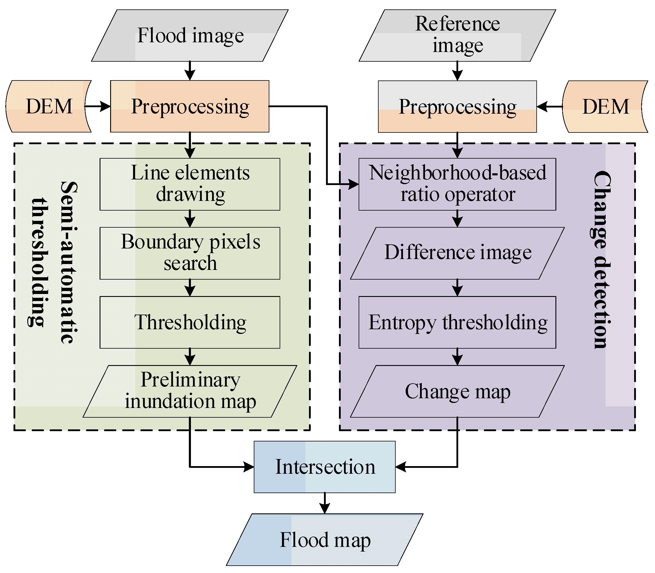
As shown in Figure 1, the proposed flood mapping framework can be divided into four main parts: (1) Pre-processing: Before further processing, geometric correction, radiometric correction, filtering, and other pre-processing steps are needed to eliminate geometric distortion, radiometric distortion, and the influence of noise as much as possible. (2) Semi-automatic thresholding: To resolve the problem of determining the optimal threshold, we propose a semi-automatic threshold extraction strategy. The method can calculate a locally optimal threshold for separating land and water with a small amount of simple manual participation. Then, the threshold is used to obtain the preliminary inundation map. (3) Change detection: In order to exclude low backscattering non-water objects, the neighborhood-based change detection method combined with the entropy thresholding is adopted to detect the changed areas. (4) Flood map generation: Considering the “low backscattering” and “high variability” characteristics of floods, the intersection of the preliminary inundation map and change map is obtained as the final flood map.
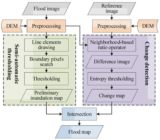
Figure 1.
Workflow of the proposed flood mapping framework.
2.1. Semi-Automatic Thresholding
Traditional image threshold segmentation algorithms [25,26] typically select the optimal threshold based on the bimodal structure of the histogram. However, the intensity histogram of a SAR image often shows a single-peak structure, so the thresholding methods that perform well in optical images are often unsatisfactory when applied directly to SAR images. In a SAR intensity image, the water bodies have obvious characteristics of low backscattering, so the section of a boundary area between land and water will show an obvious upward or downward trend. Ideally, the gradient at the boundary should be the largest. Therefore, we can use a greedy algorithm to find the pixels with the largest gradient as the boundary of land and water. The values of these pixels can be used to calculate the threshold of water and land segmentation. Based on this idea, we propose a semi-automatic thresholding algorithm with a small amount of human participation.
2.1.1. Line Element Drawing
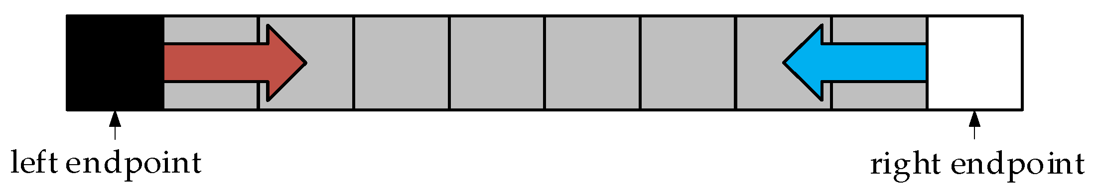
Select a typical area and draw a short line perpendicular to the boundary between land and water manually. Suppose X = (x1, x2, x3, …, xn) is the set of pixels on the line, and the number of pixels is n. Define the starting point of the line x1 as the left endpoint and the ending point xn as the right endpoint.
2.1.2. Boundary Pixel Search and Threshold Calculation
Through constructing a stepwise optimized approximation process, a greedy algorithm is used to search boundary pixels. First, the two ends of the line elements must belong to land and water because they are far from the boundary. Take them as the seed points of these two classes. Using the gradient as the comparison standard, the side with the smaller gradient is merged one pixel forward. The left and right sides meet after some pixel merging, and the pixels where they meet are identified as the boundary between land and water. Figure 2 shows an example of a boundary line pixel search. The two endpoints of the line are seen as seed points, and pixels are merged from both ends towards the middle. During the merging process, the gradient of adjacent pixels at each end is calculated. The gradients obtained are compared, and one pixel is merged forward from the end with the smaller gradient. After multiple merging iterations, the two ends eventually meet, and the average value of the two points at the meeting location is considered as the final threshold for distinguishing between land and water.

Figure 2.
Boundary line pixel search.
Suppose the gradient function of adjacent pixels from the left to the right is GL and the one from the right to the left is GR. Although the principle of the two gradient functions is the same, the definition of the function is slightly different because of the opposite direction of pixel merging. We define the gradient function GL as follows:
where ML,k−1 denotes the weighted mean from the first pixel to the k − 1st pixel, k ∈ [2, n − 1], ML,1 = x1, and
As can be seen from Equation (2), in the weighted mean of the first k pixels, the kth pixel takes up half of the weight, while the weighted mean of the first k − 1 pixels takes up another half of the weight. By expanding Equation (2), it is easy to see the weight of each pixel:
Affected by speckle noise, if the difference between adjacent pixels |xk+1 − xk| is taken as the gradient, outliers may appear, which will interfere with the search of boundary pixels. Therefore, a weighted gradient calculation method is adopted here. When a pixel is a noise point, the influence of noise on the gradient is weakened by the weighted mean. The pixels closer to xk will contribute more to the gradient, while pixels farther away from xk contribute less, reducing the calculation bias as much as possible.
The gradient function GR can be defined by
where MR,k+1 denotes the weighted mean from the last pixel to the k + 1st pixel in reverse order, k ∈ [n − 1, 1], Mn = xn, and
By expanding Equation (2), we can obtain
When the left and right sides meet, the mean value of (xi, xi+1) at the boundary is taken as the final threshold T. The preliminary inundation map FP is obtained by using the final threshold T.
This method can find a threshold that is close to the local optimal solution but not necessarily a global optimal solution. In order to approximate the global optimal solution, several typical regions can be selected for drawing lines, and then the mean value of multiple thresholds can be used as the global segmentation threshold.
In fact, due to slight variations in water bodies under different circumstances, the segmentation results are often not ideal, even if the global threshold is used. In this case, multi-threshold segmentation is a better choice. For this purpose, the image can be divided into several regions of interest (ROIs), and then each region can be segmented by the above single thresholding method. Finally, multiple segmented ROIs are combined to obtain the final result, realizing multi-threshold segmentation.
2.2. Change Detection
In general, change detection can be divided into two steps: (1) generation of difference image using images from different periods; (2) extraction of changed regions through binary segmentation of the difference image, separating the changed and unchanged regions.
2.2.1. Generation of Difference Image
The traditional methods of generating the difference image usually use difference, ratio, or logarithmic ratio, and they are mostly pixel-based. Although the SAR image has been filtered, speckle noise can hardly be eliminated completely. In order to reduce the influence of noise as much as possible, the neighborhood-based ratio (NR) operator [37], which considers spatial information, is used to obtain the difference image. The NR operator is defined as follows:
where D(x) is the value of pixel x in difference image, I1 and I2 are the flood and reference images, respectively, is the neighborhood of pixel x, ∂ is the measure of heterogeneity between I1 and I2, is the variance of pixels in the neighborhood, and μ(x) is the mean in the neighborhood.
The higher the value of ∂, the greater the heterogeneity of the neighborhood. When the heterogeneity in the neighborhood is large, the central pixel x plays a dominant role in the estimation of D(x). When the heterogeneity is small, it indicates that there is little difference between the center pixel and the adjacent pixel, and the neighborhood pixel plays a dominant role.
2.2.2. Extraction of Changed Regions
When the difference image is obtained, the changed regions can be clearly distinguished visually. However, due to the influence of speckle noise, directly using the thresholding method does not yield ideal segmentation results. Through experiments, it was found that conventional SAR filtering methods did not perform well in dealing with noise on difference images. For this situation, we propose using superpixel segmentation to improve image quality. Through merging adjacent homogeneous pixels into the same region and dividing heterogeneous pixels into different regions, and replacing the values of all pixels in the region with the mean, the noise is suppressed while the detailed information is maintained. Then, inspired by [46], the entropy thresholding method [44] is used to extract the change areas, and the change map FC is obtained.
The generalized statistical region merging (GSRM) segmentation algorithm [41] does not rely on the probability distribution assumption of the data and has good segmentation effect and high execution efficiency. Since this algorithm is a conventional segmentation algorithm, we have improved it for superpixel segmentation. The process of the modified GSRM superpixel segmentation algorithm is as follows:
- (1)
- For any input image I, assume the number of input channels is k (in this paper, the input image is the difference image, and k = 1). Using the 8-neighborhood estimation template shown in Figure 3, calculate the gradient between adjacent pixel pairs p and p’ based on Equation (9), and sort the gradient values in ascending order.where ||·|| denotes the 1-norm. Since the number of channels is k, p is a vector. The calculation rule for vector division is as follows:
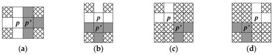 Figure 3. Eight-neighborhood gradient estimation templates with p as the central pixel and p’ as the adjacent pixel. The pixel estimation of p and p’ is computed in the Manhattan distance d = 1. (a) left-right template; (b) up-down template; (c) top-left and bottom-right template; (d) top-right and bottom-left template.
 - (2)
- Determine whether the pixel pairs p and p’ belong to the same region in sequence based on the sorted gradient order. If they belong to different regions, i.e., R(p) ≠ R(p’), the merging predicate P(R(p), R’(p’)) is calculated using the criteria of Equation (11). If the result is true, and the total pixel number of R and R’ is less than a threshold of the maximum superpixel size Smax, then R(p) and R’(p’) are merged.whereand denotes the average of all pixels in region R, |R| denotes the pixel number in region R, δ is the maximum probability when P(R, R’) = false, which is usually set to δ = 1/(6e4|I|), and Q controls the segmentation scale of the image I, which is usually set to 32. The larger the Q, the finer the segmentation, and vice versa.
- (3)
- Postprocessing [42]: Set a gradient threshold Gth and two quantity thresholds Nmin and Nmax. For any region R in the segmentation result, if |R| < Nmin, merge R into its most similar adjacent region RAdj(R). If |R|[Nmin, Nmax), the gradient GR between R and RAdj(R) is calculated according to Equation (9). If GR < Gth, region R is merged into RAdj(R).
2.3. Flood Map Generation
Flood will be mixed with non-flood objects in both the preliminary inundation map and the change map. However, there are some differences in their backscattering properties and variation properties. These differences help us to make a fine extraction of floods. The preliminary inundation map contains all the objects with the characteristics of “low backscattering”, such as permanent water, floods, airports, and roads, and the change map contains all the objects with the characteristics of “high variability”, such as vegetation, buildings, and floods. It can be found that floods have both the above characteristics. By using these two kinds of information comprehensively, the flood regions can be extracted accurately. Based on the rules of simple and fast, the intersection of the preliminary inundation map FP and the change map FC is taken as the final flood map F, which can be expressed by
F = FP ∩ FC
2.4. Evaluation Criterion
For the quantitative evaluation, the false alarm rate (FAR), missing alarm rate (MAR), detection rate (DR), overall accuracy (OA), and the Kappa coefficient are used to verify the performance of the proposed method. When the ground truth is available, these indicators can be expressed as follows:
where true positive (TP) denotes the number of changed points that are detected correctly; true negative (TN) denotes the number of unchanged points that are detected correctly; false positive (FP) denotes the number of unchanged points that are detected incorrectly; false negative (FN) denotes the number of changed points that are detected incorrectly; and N is the total number of points.
3. Experiments and Analyses
3.1. Study Area and Data
Our main study area is the Wharfe and Ouse River basin in York, UK. This area has the ground truth map from the EMSR150 case [47], which was published by Copernicus Emergency Management Service (EMS). In order to verify the applicability of the semi-automatic thresholding algorithm, the Chaohu lake of Anhui Province in China was also selected as another study area. Due to a lack of ground truth map, we selected two small regions and drew the ground truth maps according to the original SAR and quasi-synchronous optical images.
Heavy rain and bad weather caused severe flooding in York in December 2015, while Chaohu experienced a catastrophic flood due to a long-term torrential rain in August 2020. In addition to rivers and farmlands, York also contains large urban areas, roads, and airports. The objects in Chaohu are mainly lakes, rivers, and farmlands. These different features of ground objects are beneficial to test the performance of the proposed method.
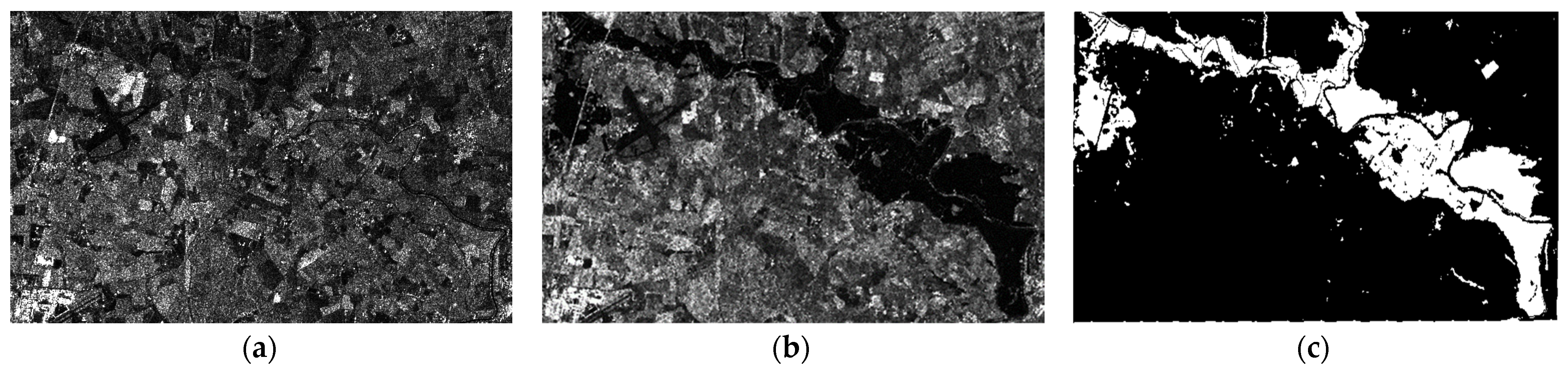
For the York experimental region, we selected Sentinel-1A single-look complex (SLC) SAR imagery, with IW imaging mode and VV polarization. Sentinel-1 has the advantages of a short revisit cycle and wide coverage, coupled with four imaging modes of IW, SM, WV, and EW. In the EMSR150 case, the image used to generate the ground truth map was acquired by Radarsat-2. Details about the York data set are listed in Table 1. The reference SAR image, flood SAR image, and ground truth map are shown in Figure 4. The image size is 550 × 1163 pixels to match the ground truth map and facilitate presentation.

Table 1.
Details about the York data set.
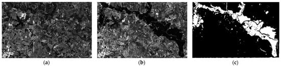
Figure 4.
York data set: (a) reference SAR image; (b) flood SAR image; (c) ground truth map.
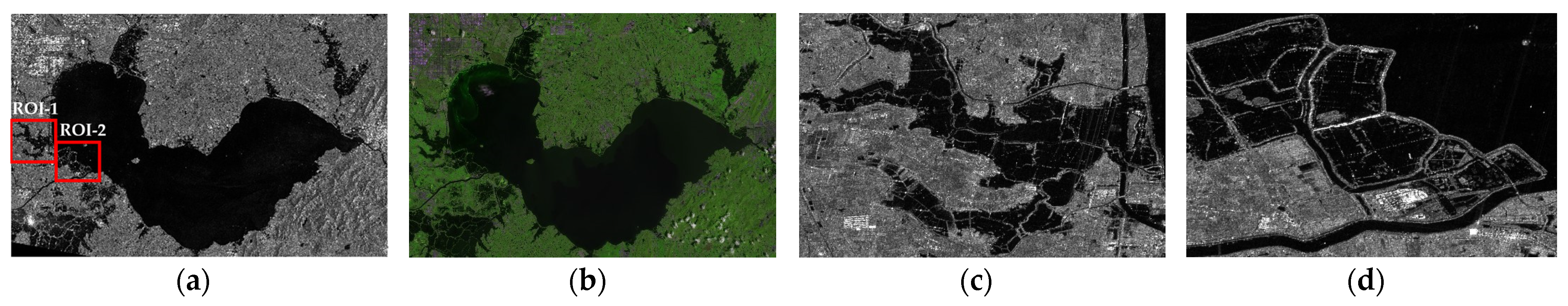
A GF-3 SLC SAR image, acquired in FSII imaging mode with HH polarization, was chosen for the Chaohu experimental area. GF-3 has a revisit period of 26 days, up to 12 imaging modes, and a spatial resolution of up to 1 m. The FSII imaging model has a spatial resolution of 10 m. For the sake of clear presentation and easy analysis, two sub-areas, ROI-1 and ROI-2, with image sizes of 561 × 696 pixels and 507 × 599 pixels, were chosen respectively for the preliminary extraction of flood. Details about the Chaohu data set are listed in Table 2. The flood SAR image, flood optical image, and the two ROI areas are shown in Figure 5. It is important to mention that the GF-3 and Sentinel-1 A data used in the two study areas are both C-band SAR data. Additionally, research has demonstrated that co-polarization (HH, VV) SAR imagery is more suitable for flood mapping compared to cross-polarization (VH, HV) imagery. This is because the differentiation between water and non-water backscattering characteristics is more pronounced in the co-polarization channels. It offers particular advantages in identifying open water bodies and inundated areas [48], as well as distinguishing flooded forests from non-flooded ones [49]. In this paper, we selected the co-polarization data, VV and HH, for the experiment.
Table 2.
Details about the Chaohu data set.
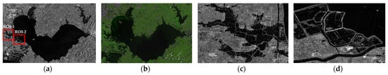
Figure 5.
Chaohu data set: (a) flood SAR image; (b) flood optical image; (c) ROI-1; (d) ROI-2.
The two SAR data sets were both preprocessed by ENVI 5.6 software, including orthographic correction and radiometric correction with global digital elevation model (DEM) data. The selected DEM is the global 30M NASADEM data released by NASA [50]. The refined Lee filter [51] with a 3 × 3 window was selected to suppress speckle noise while preserving details.
3.2. Experimental Results for York
The flood mapping framework was implemented based on PIE-SDK 6.0 and C#. First, four lines were drawn in the flood image, and the final threshold was T = 0.032189. As shown in Figure 6, it can be found that the intensity histogram shows a bimodal structure after truncation (deleting values greater than 0.4) and linear stretching (y = (x − min)/(max − min)). The position of T (its value has changed due to image enhancement) in the histogram is not at the bottom of the valley. In fact, if the threshold is at the bottom of the valley, the segmentation effect is usually not ideal. This is also a challenge encountered when using thresholding methods for flood extraction from SAR images.
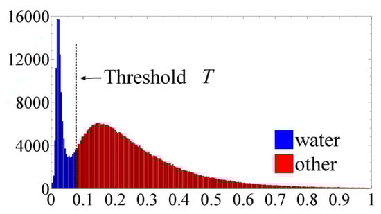
Figure 6.
The position of T in the intensity histogram of flood SAR image in York.
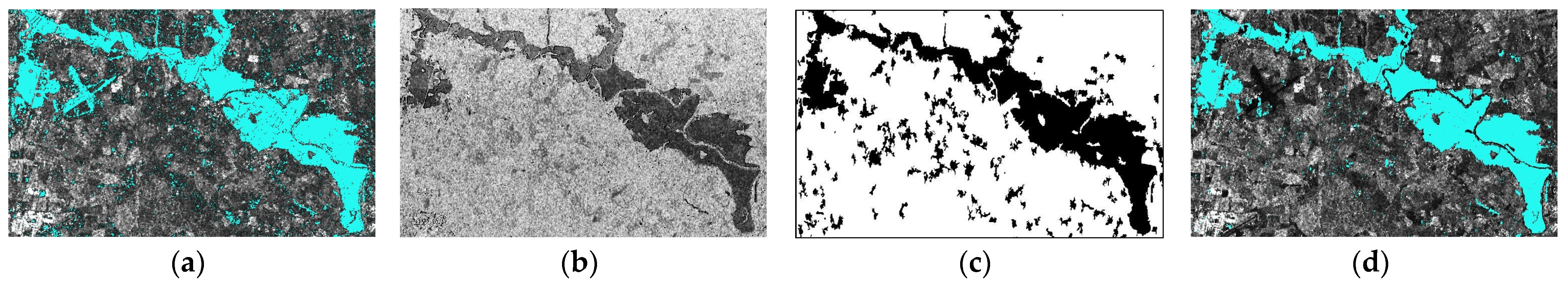
According to the threshold T, the preliminary inundation map was obtained. As shown in Figure 7a, most of the “floods” were extracted. In addition, the airport in the upper left and the permanent water bodies were also detected. Then, The NR operator with a 3 × 3 window was used to generate the difference image. As shown in Figure 7b, the changing areas on the difference image display a dark hue, while the land areas have many gray patches. These patches were caused by a variety of factors, including noise, changes in vegetation, and buildings. Compared with the preliminary inundation map (Figure 7a), the airport is not seen in the difference image (Figure 7b). However, some ground objects with high backscattering in the change map (Figure 7c) are filtered out in the preliminary inundation map. By combining the two, the final flood map is shown in Figure 7d. It can be found from Figure 7d that the large false detection areas in the preliminary inundation map and the misclassification phenomenon in the change map were effectively suppressed.
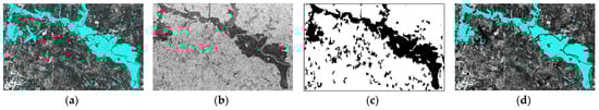
Figure 7.
Experimental results of the proposed framework: (a) preliminary inundation map; (b) difference image; (c) change map; (d) flood map.
3.3. Experimental Results for Chaohu
In addition to the proposed method, two classical thresholding segmentation methods, Otsu and K&I, were also chosen for the two study areas of Chaohu. Since the SAR intensity image follows a negative exponential distribution, there is no obvious trough in the histogram. Consequently, image enhancement needs to be applied for better effect before using Otsu and K&I [52]. When performing histogram statistics, considering the characteristics of traditional thresholding approaches, the gray scales of ROI-1 and ROI-2 were divided into 255 levels. Although the semi-automatic thresholding method does not require image enhancement, all methods are processed on the image after truncation and linear stretching in order to facilitate comparison.
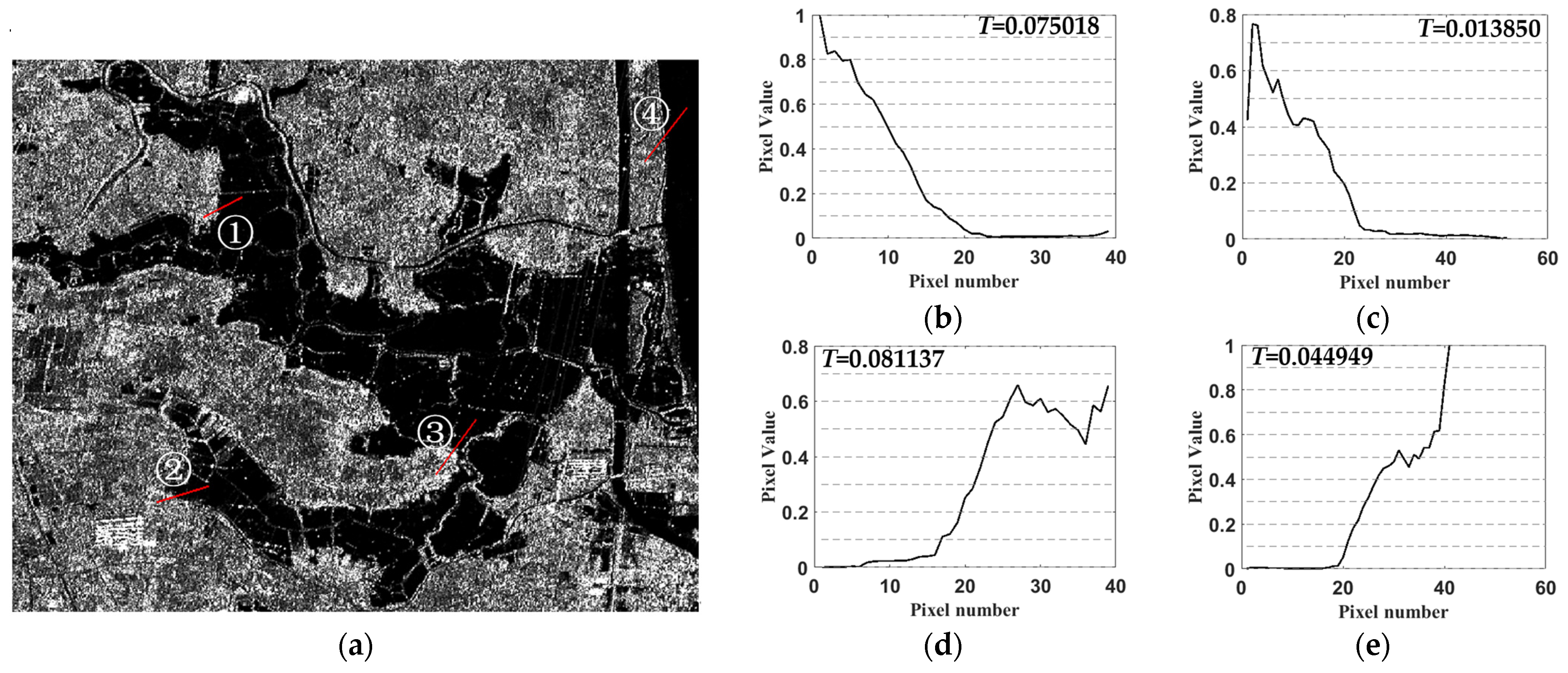
In theory, when the semi-automatic thresholding method is used for water extraction, the more lines that are drawn, the closer the threshold is to the global optimal value. However, in practical application, when the number of lines is 4–6, good segmentation results can be obtained. In this paper, four lines were drawn for both ROI-1 and ROI-2. The positions of the four lines drawn in ROI-1 are shown in Figure 8a. The profiles of these lines are shown in Figure 8b–e, from which we can see that there are great differences between water and land, but the boundary is not obvious. This is because the transition between land and water is not a step of sudden change but a slope of gradual change. In addition, the difference of thresholds between land and water boundaries in different regions is also significant.
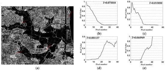
Figure 8.
Positions and profiles of the four manually drawn lines in ROI-1. (a) Positions and numbers of the manually drawn lines. (b) Profile of ①; (c) profile of ②; (d) profile of ③; (e) profile of ④.
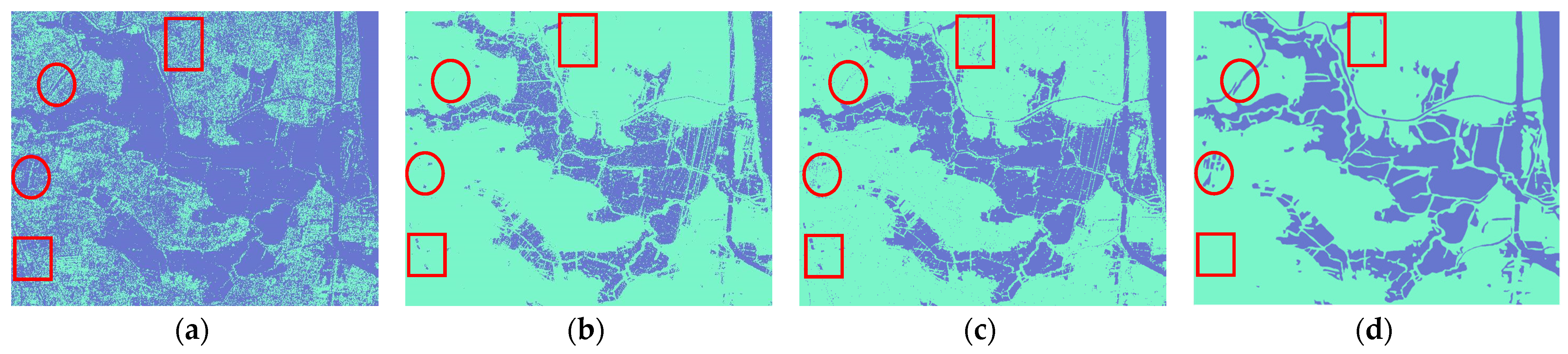
Eventually, the segmentation thresholds and extraction results of water bodies were obtained successively by different methods, as shown in Table 3 and Figure 9 and Figure 10. The ground truth maps were delineated based on the original SAR and Landsat-8 OLI optical image from adjacent periods. The water detection accuracies are listed in Table 4 and Table 5.
Table 3.
The segmentation thresholds for Chaohu.
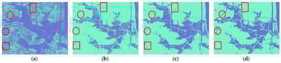
Figure 9.
Experimental results of ROI-1. (a) Otsu; (b) K&I; (c) semi-automatic thresholding; (d) ground truth map.
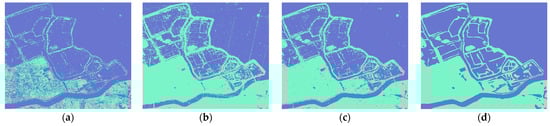
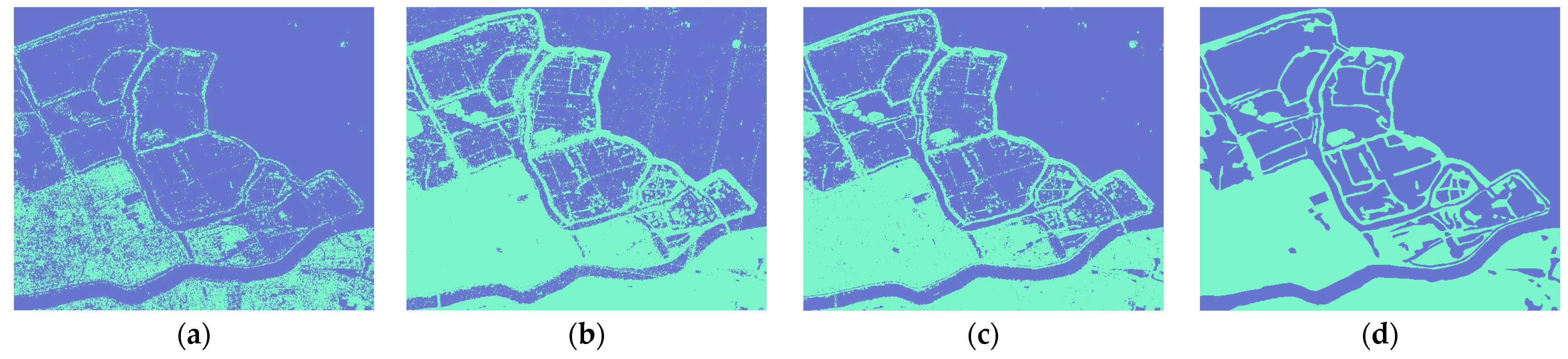
Figure 10.
Experimental results of ROI-2. (a) Otsu; (b) K&I; (c) semi-automatic thresholding; (d) ground truth map.
Table 4.
Water detection accuracies of different methods (ROI-1).
Table 5.
Water detection accuracies of different methods (ROI-2).
From the results of ROI-1 shown in Figure 9, there is a significant difference between the Otsu threshold and others, and the performance of Otsu segmentation results is the worst. Although its DR is as high as 98.47% and its MAR is very low, its FAR is much higher than other methods, resulting in low OA and Kappa. Combining with Figure 9a, we can know that the threshold of Otsu is too large, leading to serious false detection phenomena. On the contrary, the K&I method has the lowest DR and FAR and the highest MAR, which is up to 30.62%. This indicates that the threshold of the method is too small, resulting in an ordinary accuracy of the method. This is consistent with the results shown in Figure 9b. Compared with Figure 9d, obvious omissions can be seen in Figure 9b, such as the elliptical regions. In Figure 9c, although there are some false alarms (the rectangular regions) and missed detection (the elliptical regions) phenomena at the same time, the result is the closest to Figure 9d. In Table 4, all the indexes of the proposed semi-automatic thresholding method are balanced and close to the best values, so the final OA and Kappa are the highest.
The results of ROI-2 shown in Figure 10 are similar to ROI-1. Table 5 shows that the Otsu method still obtains the highest DR and FAR and the lowest MAR, OA, and Kappa, indicating that its threshold is still too high. Large areas of land are identified as water bodies in Figure 10a. The K&I method resulted in the lowest DR and FAR and the highest MAR, indicating the threshold is too low. It can be seen from Figure 10b that some water bodies are mistakenly detected as land. Consequently, its accuracy is still at the medium level. The performance of the proposed semi-automatic thresholding method is still balanced in all indicators. It can also be seen from Figure 10c that the water extraction effect of this method is the best.
3.4. Comparison with Other Methods
To further verify the effectiveness of the proposed framework, it was compared with five other methods: K-means, decision tree (DT), rule-based object-oriented classification (RBOO), support vector machine (SVM), and neural net (NN). These methods are selectable flood extraction schemes in ENVI 5.6 software. K-means belongs to unsupervised classification and does not need other manual operation except parameter setting. The DT method is based on the a priori knowledge of experts. It has a simple principle and fast calculation speed. Based on the rules of simplicity and efficiency, K-means and DT were considered. In order to prove the accuracy of the proposed method, some popular image processing algorithms including RBOO, SVM, and NN were used as comparative algorithms. The classification principle of RBOO is similar to DT, but it adds an image segmentation step, which not only suppresses noise but also adds the object size information, so its classification effect is usually better. SVM and NN both have good adaptability in image classification and can often obtain good classification results under various circumstances.
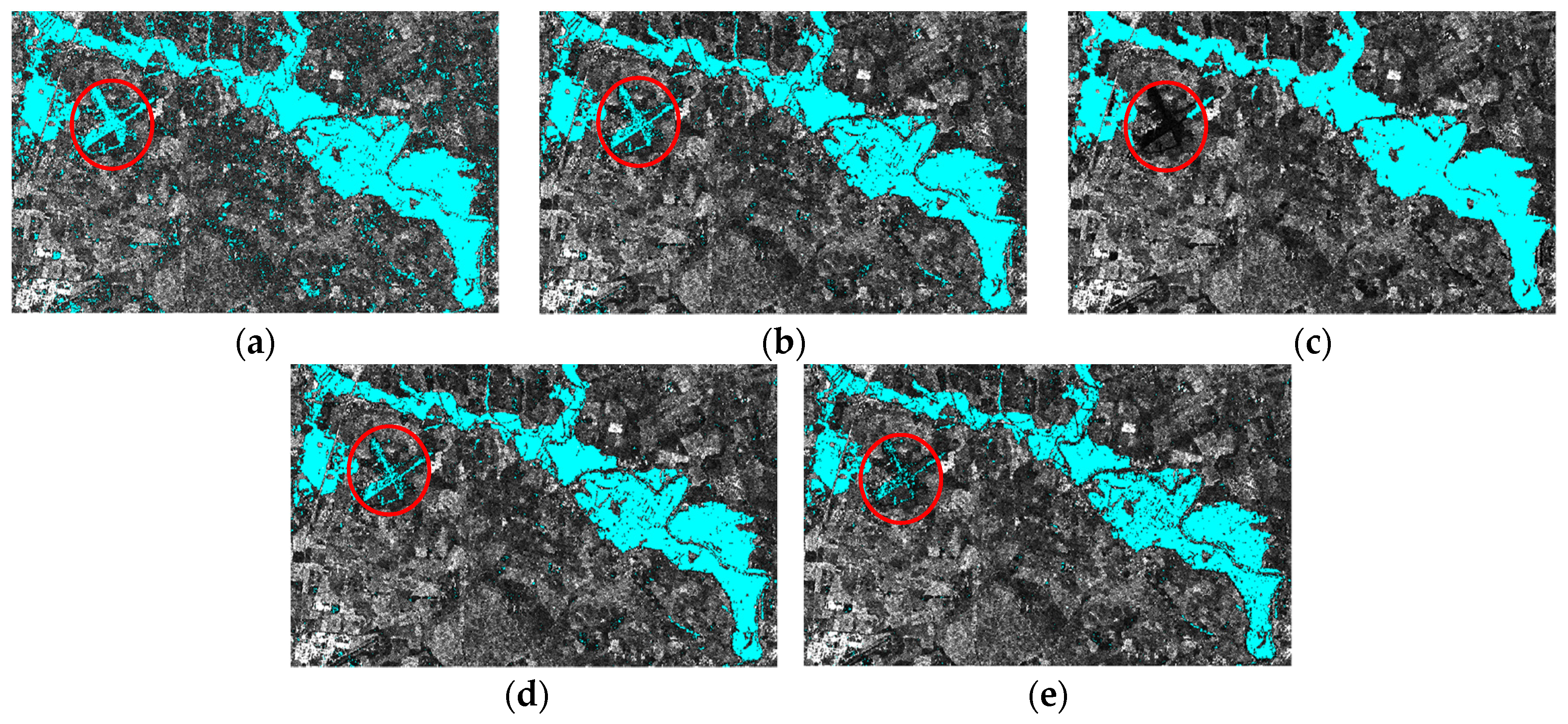
By trying different parameters, the best results obtained by each method are taken as the final results, which are shown in Figure 11. The K parameter in K-means was 6, and the maximum iterations were 7. SDWI (Sentinel-1 Dual-Polarized Water Index, SDWI = ln(10 × VV × VH) − 8) [53] was chosen in the DT method. In the RBOO method, the segments with average gray values less than 0.033 were defined as water, and the texture kernel size was 3. In the NN and SVM methods, four land cover types with different gray levels (very bright land such as buildings and tall vegetation, bright land such as low vegetation, dark land such as bare soil and road, and water) are classified. By comparing Figure 11, Figure 7d and Figure 4c, it can be found that the result obtained by the proposed framework is the closest to the ground truth map. Except for the proposed algorithm and RBOO, the rest of the algorithms misclassify the airport (the elliptical region) as inundated terrain.
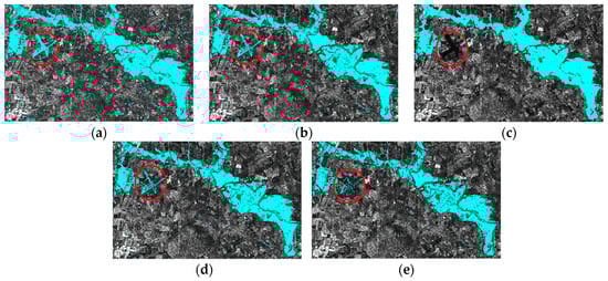
Figure 11.
Flood maps obtained by different methods: (a) K-means; (b) decision tree (DT); (c) rule-based object-oriented classification (RBOO); (d) neural network (NN); (e) support vector machine (SVM).
In order to quantitatively evaluate the accuracy of flood extraction, the evaluation indicators of different methods are calculated and shown in Table 6.
Table 6.
Flood detection accuracies of different methods.
Table 6 shows that the OAs of all algorithms exceed 90%. K-means has the third best DR and MAR, but its FAR is the worst, resulting in the worst OA and the worst Kappa. DT has worse DR and MAR than K-means, but its FAR is lower, and therefore its OA is the second worst and its Kappa is the third worst. Compared with DT, RBOO further suppresses noise through segmentation and can rule out the airport by its features, so its indicators are better than DT, and OA reaches 94.82%, second only to the proposed algorithm. NN and SVM have higher or lower indicators, but their OA and Kappa are inferior to RBOO and the proposed algorithm. All the indicators of the proposed algorithm are the best.
If parameter setting is considered, all algorithms, including K-means, require human intervention. Therefore, it is unrealistic to calculate the running time of each algorithm. However, based on the same data and software and hardware environment, the time consumed by the same operator (familiar with algorithms and processes but not data) using different methods for flood extraction is comparable. We conducted several experiments on the six comparison algorithms, and the time consumed by each algorithm is shown in Table 7. Because all algorithms need pre-processing, the time consumed by this step is not counted. In the case of not being familiar with the data, operators often achieve unsatisfactory results after the first parameter setting and manual operation. It often takes a lot of trial and error to obtain the desired result. Therefore, trial and error times are also taken as statistical indicators in this paper. As can be seen from Table 7, K-means has the fastest speed. DT and RBOO take the longest time because a large number of rule thresholds need to be manually determined, with repeated trial and error. NN and SVM have the least number of trials and errors, and the total spent time is moderate. Because the proposed method does not need parameter setting and has simple manual operation and few trial and error times, the time consumption is second only to K-means.
Table 7.
Flood detection time of different methods.
4. Discussion
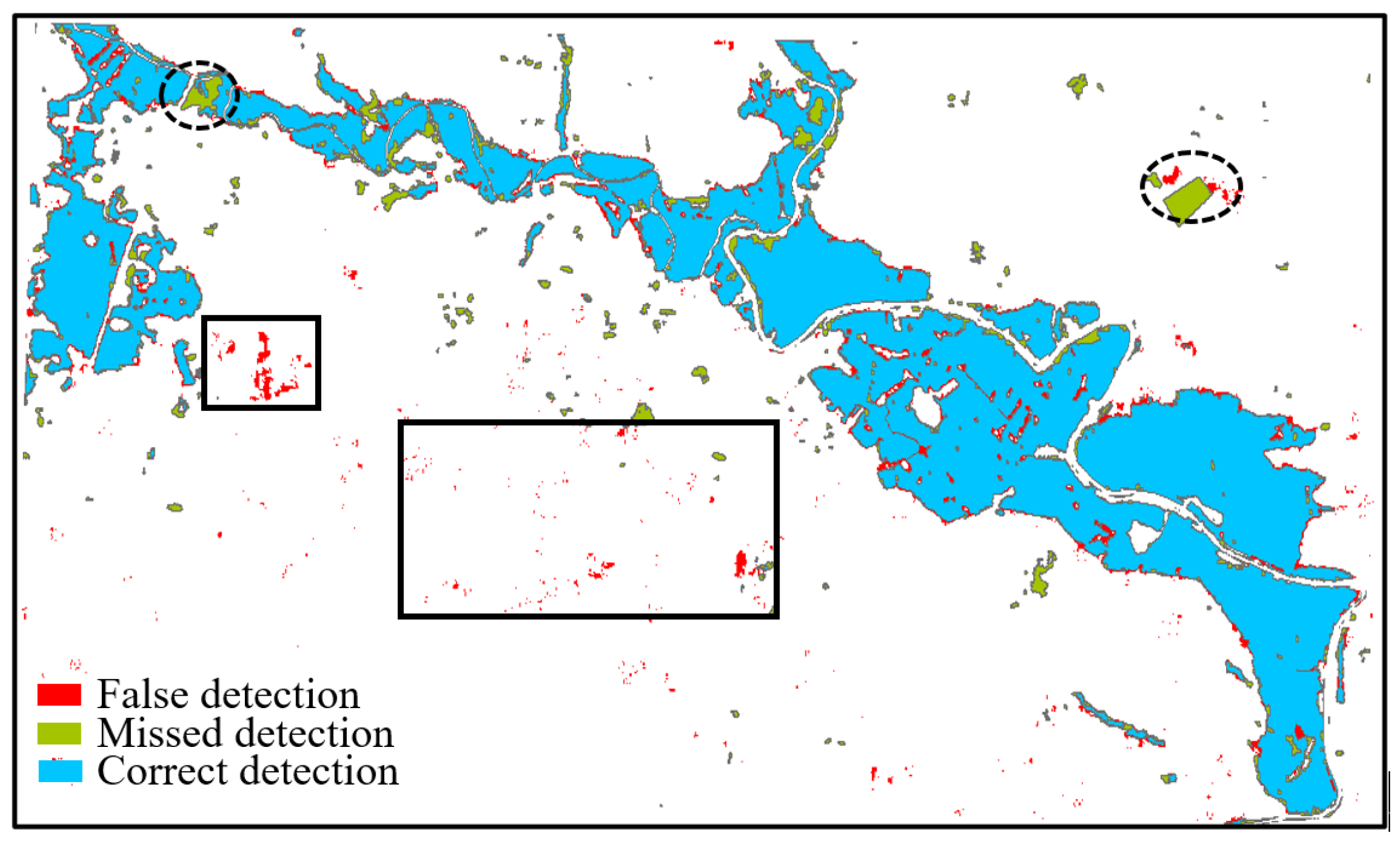
In order to display and analyze the result obtained by our method more clearly, the comparison map between the flood map and the ground truth map is shown in Figure 12. From the map we find that the missed detection area in the black dotted ellipse on the upper left is caused by change detection. The quality of change detection is not only affected by the principle of the algorithm but also largely depends on the selected reference image. The selection of the reference image in this paper adheres to the following criteria: (1) the same or similar imaging parameters, such as band, polarization mode, incident angle, etc.; (2) close imaging time to ensure similar vegetation growth and climate conditions.

Figure 12.
Comparison of flood map and ground truth map in York area.
The missed detection area in the dotted ellipse on the upper right shows a regular polygonal outline in Figure 12. This patch was marked as inundated terrain in the ground truth map. However, no ground objects with the water characteristics were found in the same position of the flood image (Figure 4b). This may be due to the ground truth map coming from different sensors and being obtained by the semi-automatic method [4]. This area is also included in the calculation of MAR. If this block of water is removed, the MAR will decrease.
In addition to the missed detection, there are some false alarms in Figure 12, as shown in the rectangular boxes. Among them, the false alarm regions in the small rectangle are larger than those in the big rectangle. By comparing the three images in Figure 4, it can be seen that these regions are low backscattering regions of change, whose characteristics are consistent with floods, so they are recognized as floods. The false alarm regions in the big rectangle are smaller and broken and also are low backscattering regions of change. However, due to their small areas, it is difficult to determine whether the changes are caused by rain puddles or by noise. Although these false alarms can be filtered out by segmenting the flood image and setting a minimum segmentation size threshold, we choose to retain this information in the case of uncertainty. On the one hand, the emergency managers generally pay more attention to the large flood areas than the small broken areas. Therefore, these small areas have little impact on flood mapping applications. On the other hand, these small areas may be puddles caused by rainfall, and their quantity and distribution may also help managers make decisions.
5. Conclusions
In order to quickly extract water from SAR images acquired during flood and exclude permanent water, we propose a flood mapping framework that combines semi-automatic thresholding and automatic change detection. The framework takes full advantage of the low backscattering and high dynamic variation of floods and only requires pre-prepared DEM and reference images, without the need for ground auxiliary data. Experiments of two real SAR data sets in the flood area demonstrate that the proposed framework has the following advantages: (a) The semi-automatic thresholding algorithm can extract the water accurately and quickly without parameter setting and multiple iterations. Because the threshold calculation process is not related to the image size, but only to the length and number of lines drawn, the larger the image that is processed, the more obvious its efficiency advantage. (b) The object-based change detection algorithm can extract inundation areas while excluding permanent water bodies and speckle noise. (c) By intersecting the preliminary inundation map with the change map, invariable ground objects with low backscattering and variable ground objects with high backscattering can be excluded, and a high-accuracy flood map can be obtained efficiently. Although the experiments show that the proposed framework has better comprehensive performance than other comparison methods in terms of accuracy and efficiency, the automation of the threshold calculation process is still worthy of further study, since human intervention can reduce the efficiency and objectivity of processing.
Author Contributions
Conceptualization and methodology, F.L.; experimentation and validation, Y.Z., J.Z. (Jinqi Zhao) and X.H.; writing—original draft preparation, X.H. and Y.Z.; writing—review and editing, F.L., Y.Z., J.Z. (Jinqi Zhao) and H.S.; project administration, F.L.; funding acquisition, F.L., H.S., N.Z. and J.Z (Jianfeng Zha). All authors have read and agreed to the published version of the manuscript.
Funding
This research was funded by the National Natural Science Foundation of China, grant numbers 42301412, 41977220, and U22A20569; the Xinjiang Key Research and Development Special Task, grant number 2022B03003-4; the open fund of Laboratory of Target Microwave Properties grant number 2022-KFJJ-003.
Data Availability Statement
The datasets presented in this paper can be obtained through http://data.cresda.cn/#/home (accessed on 10 June 2024) and http://emergency.copernicus.eu/ (accessed on 10 June 2024).
Acknowledgments
The authors would like to thank the anonymous reviewers and the editors for their insightful comments and helpful suggestions for improving the quality of our manuscript.
Conflicts of Interest
The authors declare no conflicts of interest.
References
- He, X.; Zhang, S.; Xue, B.; Zhao, T.; Wu, T. Cross-Modal Change Detection Flood Extraction Based on Convolutional Neural Network. Int. J. Appl. Earth Obs. Geoinf. 2023, 117, 103197. [Google Scholar] [CrossRef]
- Shen, X.; Wang, D.; Mao, K.; Anagnostou, E.; Hong, Y. Inundation Extent Mapping by Synthetic Aperture Radar: A Review. Remote Sens. 2019, 11, 879. [Google Scholar] [CrossRef]
- Ajmar, A.; Boccardo, P.; Broglia, M.; Kucera, J.; Giulio-Tonolo, F.; Wania, A. Response to Flood Events. In Flood Damage Survey and Assessment; American Geophysical Union (AGU): Washington, DC, USA, 2017; pp. 211–228. ISBN 978-1-119-21793-0. [Google Scholar]
- Amitrano, D.; Di Martino, G.; Iodice, A.; Riccio, D.; Ruello, G. Unsupervised Rapid Flood Mapping Using Sentinel-1 GRD SAR Images. IEEE Trans. Geosci. Remote Sens. 2018, 56, 3290–3299. [Google Scholar] [CrossRef]
- Sui, H.; An, K.; Xu, C.; Liu, J.; Feng, W. Flood Detection in PolSAR Images Based on Level Set Method Considering Prior Geoinformation. IEEE Geosci. Remote Sens. Lett. 2018, 15, 699–703. [Google Scholar] [CrossRef]
- Lu, J.; Giustarini, L.; Xiong, B.; Zhao, L.; Jiang, Y.; Kuang, G. Automated Flood Detection with Improved Robustness and Efficiency Using Multi-Temporal SAR Data. Remote Sens. Lett. 2014, 5, 240–248. [Google Scholar] [CrossRef]
- Anusha, N.; Bharathi, B. Flood Detection and Flood Mapping Using Multi-Temporal Synthetic Aperture Radar and Optical Data. Egypt. J. Remote Sens. Space Sci. 2020, 23, 207–219. [Google Scholar] [CrossRef]
- Bioresita, F.; Puissant, A.; Stumpf, A.; Malet, J.-P. Fusion of Sentinel-1 and Sentinel-2 Image Time Series for Permanent and Temporary Surface Water Mapping. Int. J. Remote Sens. 2019, 40, 9026–9049. [Google Scholar] [CrossRef]
- DeVries, B.; Huang, C.; Armston, J.; Huang, W.; Jones, J.W.; Lang, M.W. Rapid and Robust Monitoring of Flood Events Using Sentinel-1 and Landsat Data on the Google Earth Engine. Remote Sens. Environ. 2020, 240, 111664. [Google Scholar] [CrossRef]
- Heimhuber, V.; Tulbure, M.G.; Broich, M. Modeling Multidecadal Surface Water Inundation Dynamics and Key Drivers on Large River Basin Scale Using Multiple Time Series of Earth-Observation and River Flow Data. Water Resour. Res. 2017, 53, 1251–1269. [Google Scholar] [CrossRef]
- Jones, J.W. Improved Automated Detection of Subpixel-Scale Inundation—Revised Dynamic Surface Water Extent (DSWE) Partial Surface Water Tests. Remote Sens. 2019, 11, 374. [Google Scholar] [CrossRef]
- Lee, J.S.; Pottier, E. Overview of Polarimetric Radar Imaging. In Polarimetric Radar Imaging: From Basics to Applications; CRC Press: Boca Raton, FL, USA, 2009; pp. 1–30. ISBN 978-1-4200-5497-2. [Google Scholar]
- Voormansik, K.; Praks, J.; Antropov, O.; Jagomägi, J.; Zalite, K. Flood Mapping with TerraSAR-X in Forested Regions in Estonia. IEEE J. Sel. Top. Appl. Earth Obs. Remote Sens. 2014, 7, 562–577. [Google Scholar] [CrossRef]
- Uddin, K.; Matin, M.A.; Meyer, F.J. Operational Flood Mapping Using Multi-Temporal Sentinel-1 SAR Images: A Case Study from Bangladesh. Remote Sens. 2019, 11, 1581. [Google Scholar] [CrossRef]
- Giustarini, L.; Hostache, R.; Matgen, P.; Schumann, G.J.-P.; Bates, P.D.; Mason, D.C. A Change Detection Approach to Flood Mapping in Urban Areas Using TerraSAR-X. IEEE Trans. Geosci. Remote Sens. 2013, 51, 2417–2430. [Google Scholar] [CrossRef]
- Landuyt, L.; Van Wesemael, A.; Schumann, G.J.-P.; Hostache, R.; Verhoest, N.E.C.; Van Coillie, F.M.B. Flood Mapping Based on Synthetic Aperture Radar: An Assessment of Established Approaches. IEEE Trans. Geosci. Remote Sens. 2019, 57, 722–739. [Google Scholar] [CrossRef]
- Shen, X.; Anagnostou, E.N.; Allen, G.H.; Robert Brakenridge, G.; Kettner, A.J. Near-Real-Time Non-Obstructed Flood Inundation Mapping Using Synthetic Aperture Radar. Remote Sens. Environ. 2019, 221, 302–315. [Google Scholar] [CrossRef]
- Manavalan, R. SAR Image Analysis Techniques for Flood Area Mapping—Literature Survey. Earth Sci. Inform. 2017, 10, 1–14. [Google Scholar] [CrossRef]
- Martinis, S.; Kersten, J.; Twele, A. A Fully Automated TerraSAR-X Based Flood Service. ISPRS J. Photogramm. Remote Sens. 2015, 104, 203–212. [Google Scholar] [CrossRef]
- Huang, M.; Jin, S. Backscatter Characteristics Analysis for Flood Mapping Using Multi-Temporal Sentinel-1 Images. Remote Sens. 2022, 14, 3838. [Google Scholar] [CrossRef]
- Martinis, S.; Rieke, C. Backscatter Analysis Using Multi-Temporal and Multi-Frequency SAR Data in the Context of Flood Mapping at River Saale, Germany. Remote Sens. 2015, 7, 7732–7752. [Google Scholar] [CrossRef]
- Liang, J.; Liu, D. A Local Thresholding Approach to Flood Water Delineation Using Sentinel-1 SAR Imagery. ISPRS J. Photogramm. Remote Sens. 2020, 159, 53–62. [Google Scholar] [CrossRef]
- Bazi, Y.; Bruzzone, L.; Melgani, F. An Unsupervised Approach Based on the Generalized Gaussian Model to Automatic Change Detection in Multitemporal SAR Images. IEEE Trans. Geosci. Remote Sens. 2005, 43, 874–887. [Google Scholar] [CrossRef]
- Zhao, J.; Yang, J.; Lu, Z.; Li, P.; Liu, W.; Yang, L. An Unsupervised Method of Change Detection in Multi-Temporal PolSAR Data Using a Test Statistic and an Improved K&I Algorithm. Appl. Sci. 2017, 7, 1297. [Google Scholar] [CrossRef]
- Kittler, J.; Illingworth, J. Minimum Error Thresholding. Pattern Recognit. 1986, 19, 41–47. [Google Scholar] [CrossRef]
- Otsu, N. A Threshold Selection Method from Gray-Level Histograms. IEEE Trans. Syst. Man Cybern. 1979, 9, 62. [Google Scholar] [CrossRef]
- Gstaiger, V.; Huth, J.; Gebhardt, S.; Wehrmann, T.; Kuenzer, C. Multi-Sensoral and Automated Derivation of Inundated Areas Using TerraSAR-X and ENVISAT ASAR Data. Int. J. Remote Sens. 2012, 33, 7291–7304. [Google Scholar] [CrossRef]
- Kuenzer, C.; Guo, H.; Schlegel, I.; Tuan, V.Q.; Li, X.; Dech, S. Varying Scale and Capability of Envisat ASAR-WSM, TerraSAR-X Scansar and TerraSAR-X Stripmap Data to Assess Urban Flood Situations: A Case Study of the Mekong Delta in Can Tho Province. Remote Sens. 2013, 5, 5122–5142. [Google Scholar] [CrossRef]
- Greifeneder, F.; Wagner, W.; Sabel, D.; Naeimi, V. Suitability of SAR Imagery for Automatic Flood Mapping in the Lower Mekong Basin. Int. J. Remote Sens. 2014, 35, 2857–2874. [Google Scholar] [CrossRef]
- Bai, Y.; Wu, W.; Yang, Z.; Yu, J.; Zhao, B.; Liu, X.; Yang, H.; Mas, E.; Koshimura, S. Enhancement of Detecting Permanent Water and Temporary Water in Flood Disasters by Fusing Sentinel-1 and Sentinel-2 Imagery Using Deep Learning Algorithms: Demonstration of Sen1Floods11 Benchmark Datasets. Remote Sens. 2021, 13, 2220. [Google Scholar] [CrossRef]
- Zhao, J.; Yang, J.; Lu, Z.; Li, P.; Liu, W.; Yang, L. A Novel Method of Change Detection in Bi-Temporal PolSAR Data Using a Joint-Classification Classifier Based on a Similarity Measure. Remote Sens. 2017, 9, 846. [Google Scholar] [CrossRef]
- Wu, C.; Du, B.; Zhang, L. Fully Convolutional Change Detection Framework with Generative Adversarial Network for Unsupervised, Weakly Supervised and Regional Supervised Change Detection. IEEE Trans. Pattern Anal. Mach. Intell. 2023, 45, 9774–9788. [Google Scholar] [CrossRef]
- Zhao, B.; Sui, H.; Liu, J. Siam-DWENet: Flood Inundation Detection for SAR Imagery Using a Cross-Task Transfer Siamese Network. Int. J. Appl. Earth Obs. Geoinf. 2023, 116, 103132. [Google Scholar] [CrossRef]
- Ji, L.; Zhao, J.; Zhao, Z. A Novel End-to-End Unsupervised Change Detection Method with Self-Adaptive Superpixel Segmentation for SAR Images. Remote Sens. 2023, 15, 1724. [Google Scholar] [CrossRef]
- Paul, S.; Ganju, S. Flood Segmentation on Sentinel-1 SAR Imagery with Semi-Supervised Learning. 2021. Available online: http://arxiv.org/abs/2107.08369 (accessed on 10 June 2024).
- Ma, F.; Xiang, D.; Yang, K.; Yin, Q.; Zhang, F. Weakly Supervised Deep Soft Clustering for Flood Identification in SAR Images. IEEE Geosci. Remote Sens. Lett. 2022, 19, 4505005. [Google Scholar] [CrossRef]
- Gong, M.; Cao, Y.; Wu, Q. A Neighborhood-Based Ratio Approach for Change Detection in SAR Images. IEEE Geosci. Remote Sens. Lett. 2012, 9, 307–311. [Google Scholar] [CrossRef]
- Sumaiya, M.N.; Shantha Selva Kumari, R. Logarithmic Mean-Based Thresholding for SAR Image Change Detection. IEEE Geosci. Remote Sens. Lett. 2016, 13, 1726–1728. [Google Scholar] [CrossRef]
- Cui, B.; Zhang, Y.; Yan, L.; Wei, J.; Huang, Q. A SAR Change Detection Method Based on the Consistency of Single-Pixel Difference and Neighbourhood Difference. Remote Sens. Lett. 2019, 10, 488–495. [Google Scholar] [CrossRef]
- Akbari, V.; Anfinsen, S.N.; Doulgeris, A.P.; Eltoft, T.; Moser, G.; Serpico, S.B. Polarimetric SAR Change Detection with the Complex Hotelling–Lawley Trace Statistic. IEEE Trans. Geosci. Remote Sens. 2016, 54, 3953–3966. [Google Scholar] [CrossRef]
- Lang, F.; Yang, J.; Yan, S.; Qin, F. Superpixel Segmentation of Polarimetric Synthetic Aperture Radar (SAR) Images Based on Generalized Mean Shift. Remote Sens. 2018, 10, 1592. [Google Scholar] [CrossRef]
- Qin, F.; Guo, J.; Lang, F. Superpixel Segmentation for Polarimetric SAR Imagery Using Local Iterative Clustering. IEEE Geosci. Remote Sens. Lett. 2015, 12, 13–17. [Google Scholar]
- Lang, F.; Yang, J.; Li, D.; Zhao, L.; Shi, L. Polarimetric SAR Image Segmentation Using Statistical Region Merging. IEEE Geosci. Remote Sens. Lett. 2014, 11, 509–513. [Google Scholar] [CrossRef]
- Kapur, J.N.; Sahoo, P.K.; Wong, A.K.C. A New Method for Gray-Level Picture Thresholding Using the Entropy of the Histogram. Comput. Vis. Graph. Image Process. 1985, 29, 273–285. [Google Scholar] [CrossRef]
- Li, Y.; Martinis, S.; Plank, S.; Ludwig, R. An Automatic Change Detection Approach for Rapid Flood Mapping in Sentinel-1 SAR Data. Int. J. Appl. Earth Obs. Geoinf. 2018, 73, 123–135. [Google Scholar] [CrossRef]
- Lang, F.; Yang, J.; Li, D. Adaptive-Window Polarimetric SAR Image Speckle Filtering Based on a Homogeneity Measurement. IEEE Trans. Geosci. Remote Sens. 2015, 53, 5435–5446. [Google Scholar] [CrossRef]
- Copernicus Emergency Management Service. Directorate Space, Security and Migration, European Commission Joint Research Centre (EC JRC). Available online: http://Emergency.Copernicus.Eu/ (accessed on 10 June 2024).
- Gao, H.X.; Chen, B.; Sun, H.Q. Research Progress and Prospect of Flood Detection Based on SAR Satellite Images. J. Geo-Inf. Sci. 2023, 25, 1933–1953. [Google Scholar]
- Hess, L.L.; Melack, J.M.; Simonett, D.S. Radar Detection of Flooding Beneath the Forest Canopy: A Review. Int. J. Remote Sens. 1990, 11, 1313–1325. [Google Scholar] [CrossRef]
- NASA JPL (2020). NASADEM Merged DEM Global 1 arc Second V001 [Data Set]. NASA EOSDIS Land Processes Distributed Active Archive Center. Available online: http://doi.org/10.5067/MEaSUREs/NASADEM/NASADEM_HGT.001 (accessed on 10 June 2024).
- Lee, J.S.; Grunes, M.R.; De Grandi, G. Polarimetric SAR Speckle Filtering and Its Implication for Classification. IEEE Trans. Geosci. Remote Sens. 1999, 37, 2363–2373. [Google Scholar]
- Schmidtab, M.; Escha, T.; Kleinb, D.; Thielb, M.; Dechab, S. Estimation of Building Density Using Terrasar-X-Data. In Proceedings of the 2010 IEEE International Geoscience and Remote Sensing Symposium, Honolulu, HI, USA, 25–30 July 2010; pp. 1936–1939. [Google Scholar]
- Jia, S.; Xue, D.; Li, C.; Zheng, J.; Li, W. Study on New Method for Water Area Information Extraction Based on Sentinel-1 Data. Yangtze River 2019, 50, 213–217. [Google Scholar]


Disclaimer/Publisher’s Note: The statements, opinions and data contained in all publications are solely those of the individual author(s) and contributor(s) and not of MDPI and/or the editor(s). MDPI and/or the editor(s) disclaim responsibility for any injury to people or property resulting from any ideas, methods, instructions or products referred to in the content. |
© 2024 by the authors. Licensee MDPI, Basel, Switzerland. This article is an open access article distributed under the terms and conditions of the Creative Commons Attribution (CC BY) license (https://creativecommons.org/licenses/by/4.0/).