Article

Research on Jianghan Plain Water System Dynamics and Influences with Multiple Landsat Satellites

1
School of Remote Sensing Information Engineering, Wuhan University, Wuhan 430072, China
2
School of Cyber Science and Engineering, Wuhan University, Wuhan 430072, China
*
Author to whom correspondence should be addressed.
Remote Sens. 2024, 16(15), 2770; https://doi.org/10.3390/rs16152770 (registering DOI)
Submission received: 23 June 2024 / Revised: 25 July 2024 / Accepted: 26 July 2024 / Published: 29 July 2024
(This article belongs to the Section Remote Sensing and Geo-Spatial Science)

Abstract

:
The study of the spatio-temporal distribution and evolution trends of water resources in large regions plays an important role in the study of regional water resource planning, regional economic and social development, and water disasters. In this study, a Landsat multi-index relationship and water probability thresholding method is developed based on the Google Earth Engine (GEE) platform, which can support the integration of multiple Landsat satellites. The algorithm jointly combines multiple remote sensing metrics along with the calculation of water probability to produce an interannual water body product for the Jianghan Plain on a 20-year time series. The results indicate that the Landsat multi-index relationship algorithm used in this study has high accuracy in extracting long-term water bodies in extensive, flat terrain areas such as the Jianghan Plain, with an overall accuracy (OA) of 97.23%. By analyzing the water body products and landscape patterns, we have identified the following features: (1) From 2002 to 2021, the changes in river water bodies in the Jianghan Plain were relatively small, and some lakes experienced a shrinkage in area. Overall, there is a strong correlation between water distribution and precipitation. (2) The complexity index of water bodies shows a strong negative correlation with effective irrigation area and population, indicating a strong mutual influence between water bodies and socio-economic activities. (3) Through the study of the distribution characteristics of built-up areas and the water system, it was found that for large rivers, the larger the size of the river, the more built-up areas are nearby. Most extensive built-up areas are located near large rivers. This study contributes to providing methods and data support for urban planning, water resource management, and disaster research in the Jianghan Plain.

1. Introduction

The Jianghan Plain is surrounded by the Yangtze River and the Han River, with a flat terrain, numerous lakes, and dense river networks. The abundant water resources are an important feature of the region and have a crucial impact on its economic and social development [1,2]. The water system is not only one of the key ecological elements, but also directly affects the development of agriculture, industry, and cities in the Jianghan Plain. Clarifying the evolution law of the Jianghan Plain water system in urban development and balancing water system protection and sustainable socio-economic development can help clarify the relationship between water system evolution and urbanization, promote socio-economic development, and protect the ecological environment.
Clarifying the evolutionary pattern of the water system needs to be supported by dynamic and continuous water body monitoring data. Remote sensing has the capability of large-size continuous monitoring in both temporal and spatial dimensions, making it an important technique for water body monitoring. Water body remote sensing identification methods have evolved from manual, visual identification to semi-automatic extraction based on spectral, texture, and spatial information, and now to the popular research of high-precision extraction of water bodies based on deep learning. The overall goal is to achieve high-precision, automatic extraction of water bodies [3]. Before 2010, due to the slow development of remote sensing technology, water body extraction could only be performed through simple pixel band calculations. Zhou et al. [4] discovered the spectral feature that water bodies have a grayscale value of (TM 2+ TM 3) > (TM 4+ TM 5) in TM images. With the emergence of high-resolution remote sensing data, object-oriented water body extraction algorithms have rapidly developed since 2010. Cui et al. [5] proposed a method based on object-oriented vector constraints for high spatial resolution remote sensing image water body extraction, which can accurately extract small water body information. After 2015, active radar image-based water body extraction [6] and machine learning-based deep learning [7] methods have gradually been applied in water body extraction, and semi-automatic technologies have also matured. However, due to various factors such as cloud cover, complex terrain, shadows, and human interference, water body extraction algorithms still have certain limitations, and suitable algorithms need to be selected based on the geographic environment. Although there are water data products available both domestically and internationally, such as Joint Research Centre (JRC) Global Water Data [8] and various resolutions of land use data, deficiencies in terms of resolution and dynamic distribution of water bodies still exist.
In the study of spatio-temporal evolution of water systems, landscape indices can reflect the spatial characteristics of water system evolution from different perspectives, supporting quantitative exploration of the relationship between water system evolution and urban development. Legleiter et al. [9] and Nguyen et al. [10] emphasize the importance of comprehensively assessing the spatio-temporal changes in water systems. This involves evaluating quantitative attributes, morphological structure, spatial distribution, and connectivity. The quantitative evaluation of water system changes gained attention in the early to mid-20th century, with Horton et al. [11] proposing the law of stream quantity and length. In the 1980s, the rapid development of remote sensing and geographic information systems led to advancements in studying water systems, integrating landscape ecology, river geomorphology, and geological hydrology. Currently, researchers like Vassoney et al. [12] and Fang et al. [13] have constructed indicator systems for studying water system evolution, considering parameters such as water volume, river network density, complexity, and box dimension. Bosch et al. [14] analyzed urban land using fractal analysis and divided each agglomeration into inner and outer zones based on distance from the city center. Landscape metrics and growth modes were computed for these zones. Zhu et al. [15] explored land use and landscape pattern changes in the Liuxihe River basin from 1980 to 2015 using satellite data and land-use transition matrices. Zhai et al. [16] studied land use changes in Wuhan from 2000 to 2019 using continuous time series mapping. Fu et al. [17] analyzed the spatio-temporal evolution of urbanization in Guangxi using nighttime light data and statistical analysis. Chen et al. [18] characterized the spatio-temporal evolution of landscape patterns over the past 20 years using remote sensing and spatial analysis techniques. In recent years, the evaluation of water systems through certain indicators has also become increasingly popular. The water ecological footprint indicator was proposed by Huang et al. [19] to assess the water resource carrying capacity by measuring water resource consumption. Ecological resilience (ER) elucidates the threat of regional ecological security to ensure sustainable development [20]. Meanwhile, other water landscape indices have gradually developed.
In order to obtain reliable data on the Jianghan Plain water system over the past 20 years to support spatio-temporal evolution analysis, we chose Landsat series remote sensing images as the monitoring data source. A water extraction method was proposed based on the accurate acquisition of information about water bodies and the comprehensive utilization of Landsat 5/7/8 images. This method combines multiple remote sensing indices and water probability calculation methods to accurately extract interannual water bodies within the region. Based on this, we calculated multiple types of water landscape indices and analyzed the spatio-temporal changes and landscape pattern characteristics of the Jianghan Plain water system. In addition, we explored the relationship between water systems, socio-economic indicators, and urban built-up areas through correlation analysis, aiming to understand the evolution patterns of water systems under the background of urbanization. The research results can provide reliable data support and a methodological basis for water resource protection, land allocation planning, spatial structure adjustment, and urbanization construction.

2. Study Area and Data Sources

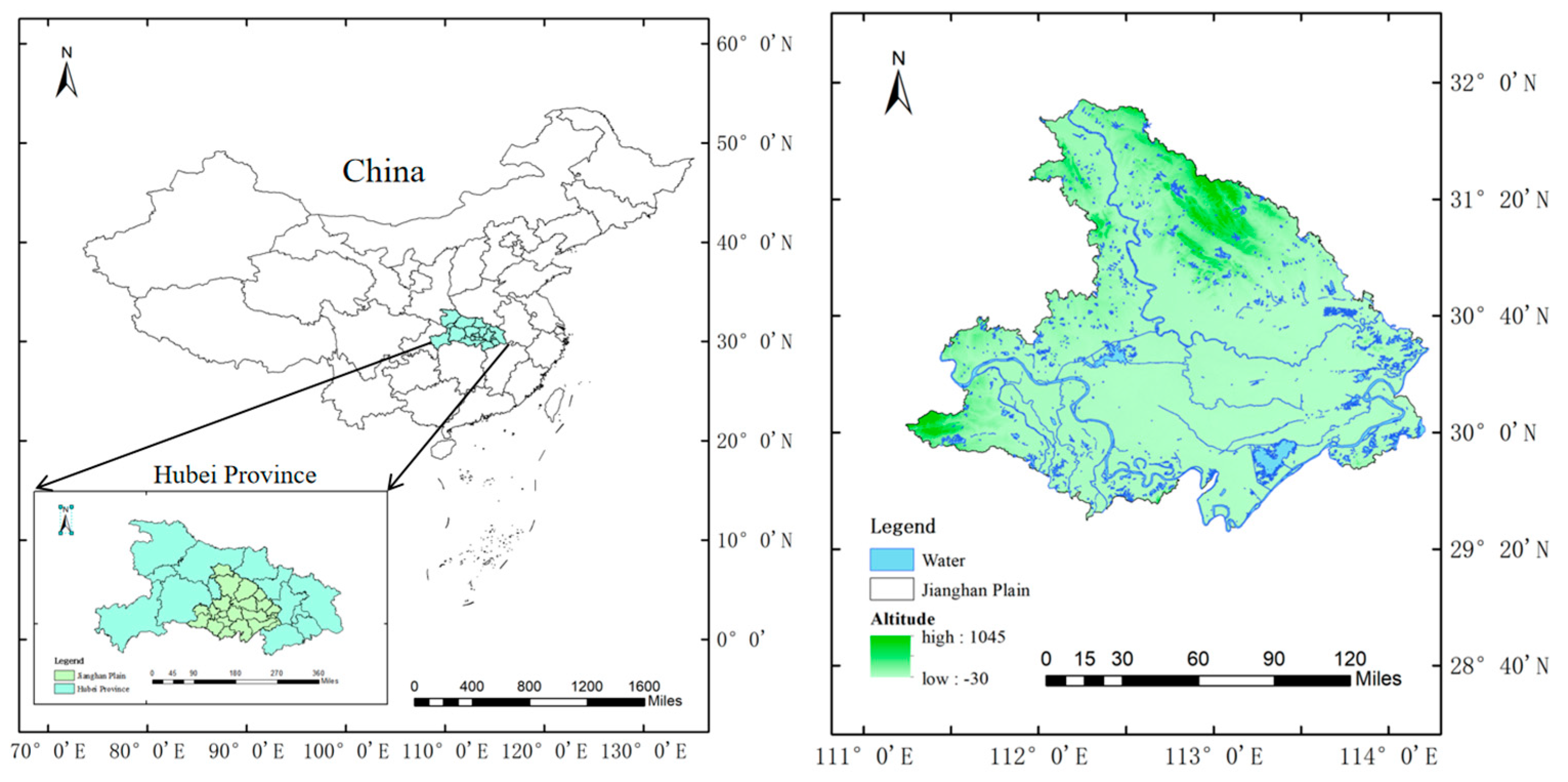
2.1. Overview of the Study Area

The Jianghan Plain is located between 29°26′N~31°37′N and 111°14′E~114°36′E, with an area of over 46,000 square kilometers. It has a subtropical monsoon climate, with distinct dry and wet seasons. The average annual temperature is about 20 °C, and the average annual precipitation is 1100–1300 mm [21]. The Jianghan Plain has a flat terrain, a dense river network, numerous lakes, and a vast water area. Originally, there were four major lakes in the Jianghan Plain: Honghu, Changhu, Sanhu, and Bailu Lake. Due to changes in the time and human activities, the water system in the basin has changed. Currently, Sanhu and Bailu Lake have disappeared, leaving Honghu, the seventh largest lake in China, and Changhu, the third largest lake in Hubei [22]. This article mainly studies the spatio-temporal distribution and the correlation analysis of all water systems in various cities within the Jianghan Plain. According to statistics, the water area of the Jianghan Plain accounts for 18% of its total area, with a lake area of 1605.4 square kilometers. The average annual runoff depth of the entire Jianghan Plain is 320–750 mm, and water resources are extremely abundant [23]. The schematic map of Jianghan Plain is shown in Figure 1.

2.2. Data Sources and Preprocessing

2.2.1. Data Sources

The boundary of this study area is the vector data of administrative divisions in the Jianghan Plain. The urban economic attribute data of the Jianghan Plain are composed of the cultivated land area, effective irrigation area, highway mileage, land area, registered residence population, permanent population, gross national product, gross domestic product of the primary industry, gross domestic product of the secondary industry, gross domestic product of the tertiary industry, and other data of 21 counties and districts in the Jianghan Plain from 2012 to 2021. The subsequent correlation analysis is conducted with the water landscape index. The Landsat series of surface reflectance (SR) datasets are generated based on the Landsat Ecosystem Disturbance Adaptive Processing System for water extraction and sampling of base maps [24]. The Sentinel series satellite imagery is an Earth observation satellite in the Copernicus program of the European Space Agency [25], used for water extraction and sampling of base maps. The Dynamic World (DW) land classification dataset was created by Google using Google Earth Engine (GEE) and AI Platform [26], mainly used for farmland screening and built-up area extraction. The JRC Monthly Water History product is a set of 30 m resolution monthly surface water monitoring maps of global surface water coverage, generated using satellite images of Landsat 5, Landsat 7, and Landsat 8 obtained from 1984 to 2020 [27]. Table 1 shows the sources and types of the above data.

2.2.2. Data Preprocessing

The economic attribute data of the Jianghan Plain used in this article mainly comes from the Hubei Provincial Bureau of Statistics. Some attribute data show annual regular changes, but there are some missing data. Therefore, spline interpolation is used to estimate the missing data value based on the trend of existing data points, ensuring the integrity and consistency of the data.
This research used the GEE platform to obtain and process images, and the implementation of the algorithm is mainly called the GEE interface implementation. Among them, the GEE image data were preprocessed, including radiometric, atmospheric, and geometric corrections [28]. To further improve data quality, it was necessary to perform cloud removal processing on the Landsat and Sentinel satellite image data. Researchers have conducted extensive work on cloud detection and removal, proposing various efficient cloud removal methods, such as multispectral synthesis [29], the optical temperature difference method, and the exponential method [30]. At present, the Landsat satellite image cloud removal method provided by the GEE platform mainly focuses on SR data cloud removal. We used pixel-quality information from Landsat 5/7/8 to detect clouds and shadows. By extracting specific pixels from remote sensing images, bit operations and conditional filtering are used to detect clouds, shadows, and cloud projection pixels, and corresponding masks are generated. Based on the mask and additional pixel value conditions, these influencing factors are excluded, and the image with the cloud, shadow, and specific pixel values removed is ultimately obtained.

3. Methods

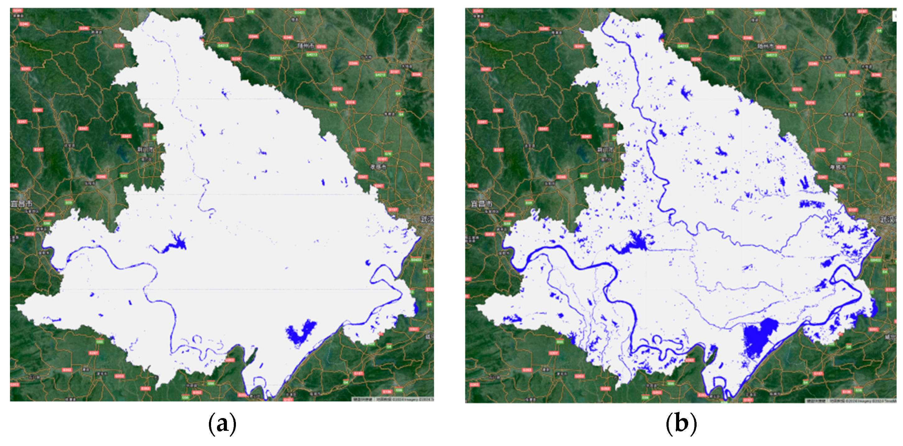
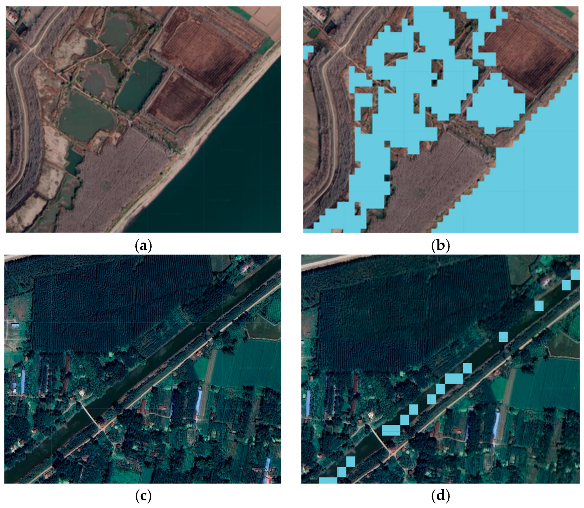
3.1. Water Body Extraction Based on Landsat 5/7/8 Multi-Index Fusion

This article aims to examine the interannual spatio-temporal evolution characteristics of the water system in the Jianghan Plain over the past 20 years. Obtaining a reliable water body range is an important basis for this research. The Jianghan Plain, characterized by its flat terrain and numerous rivers and lakes, experiences a typical subtropical monsoon climate with significant seasonal variations in water body extent. Determining the interannual average water body range to accurately represent the spatial distribution characteristics of water systems is a crucial aspect of water body extraction. Meanwhile, due to abundant water resources and a suitable climate, the distribution of paddy fields and ponds is relatively dense. Distinguishing ponds, paddy fields, and water bodies has become another challenge for water extraction. To address these issues, this article combines Landsat 5, 7, and 8 satellite sources and proposes a water body recognition method that combines multi-exponential relationships and a water body probability threshold method. The specifics of the algorithm are shown in Figure 2.
Currently, JRC Monthly Water History products [31] and DW near real-time land type water probability datasets [32] are widely recognized and well-regarded water products. However, due to the use of multi-month water body data and the extraction of interannual water body products, the JRC dataset tends to have a larger water body range and cannot accurately reflect the mean range of interannual water bodies. Although the DW dataset has a high resolution, its time series is short, which does not meet the research requirements for long time series in this article.
Considering that the time span of this study is 20 years, along with the geographical scope, topography, and climate characteristics of the Jianghan Plain, a single satellite source would be inadequate for continuous monitoring. Therefore, we selected the Landsat series satellites (Landsat 5, 7, and 8) with long-term and continuous monitoring capabilities as the data source. This choice ensures the continuity of monitoring time, and on the other hand, the differences between sensors are relatively small, making data consistency less difficult and highly reliable.
The TM and ETM+ sensors on Landsat 5 and 7, respectively, had seven multi-spectral bands, while the OLI sensor on Landsat 8 has eight 30 m bands [33], enabling accurate extraction of ground targets such as water bodies, vegetation, and buildings through the calculation of various remote sensing indices. At present, the commonly used water body indices include the Normalized Difference Water Index (NDWI), Modified Normalized Difference Water Index (MNDWI), Multi-Band Water Index (MBWI), and Automatic Water Extraction Index (AWEI), each with distinct advantages. The Jianghan Plain, characterized by flat terrain, dense vegetation, and a very developed water system and lake group, has a minimal influence of mountainous shadows but contains numerous buildings. Therefore, MNDWI was selected for water extraction, which can effectively remove the influence of residential areas, soil, etc., highlight water bodies, and distinguish between water bodies and shadows [34]. Additionally, in order to eliminate the impact of vegetation and farmland, the Normalized Difference Vegetation Index (NDVI) and Enhanced Vegetation Index (EVI) are also calculated. NDVI is primarily used to evaluate vegetation coverage and extract vegetation within the study area [35]; EVI combines vegetation and soil information by adding aerosol impedance coefficients during processing to correct atmospheric aerosol scattering and soil background effects and stably reflect the vegetation situation in the measured area [36].
Reasonable threshold segmentation based on index calculation results is essential for accurately extracting the range of water bodies. The commonly used threshold segmentation methods include Otsu, Kapur’s, and wave-by-wave threshold methods. In this paper, the Otsu method was selected for automated threshold segmentation. Automated threshold segmentation is simple, fast, accurate, and widely applicable with good practicality and adjustability. The overall algorithmic process for water extraction is shown in Figure 2.
The water body index method selects bands closely related to water body recognition by analyzing the spectral characteristics of water bodies. It constructs different water body index models and assigns corresponding thresholds to extract water body information accurately. This research combines multiple remote sensing indices to extract water information from the Landsat series SR dataset. The remote sensing indices used include NDVI, MNDWI, and EVI. These indices are calculated based on the differences in reflectance between different bands in multi-band image data. The specific calculation formulas are shown in Formula (1).
      NDVI = B N I R B R E D B N I R + B R E D       M N D W I = B G R E E N B M I R B G R E E N + B M I R E V I = 2.5 B N I R B R E D B N I R + 6 B R E D 7 B B L U E + 1
B M I R , B N I R , B R E D , B G R E E N , B B L U E represent the pixel values of the mid-infrared, near-infrared, red, green, and blue bands, respectively. Among them, Landsat 5 and Landsat 7 represent the B5, B4, B3, B2, and B1 bands, respectively; in Landsat 8, they are represented by bands B6, B5, B4, B3, and B2.
In order to eliminate the influence of vegetation and soil in the water extracted by the MNDWI, we used logical operation rules to identify water bodies. By analyzing the different combination relationships of EVI, MNDWI, and NDVI, we can determine whether the location is a water body. The calculation formula for determining conditions is shown in Formula (2).
w a t e r = 1 ,   i f ( E V I < 0.1 ) ( ( M N D W I > N D V I ) ( M N D W I > E V I ) ) 0 , Other
EVI can stably reflect the vegetation situation in the measured area. As there is almost no vegetation in water-covered areas, an EVI less than 0.1 is taken to extract areas with minimal vegetation. MNDWI reduces the impact of soil and buildings, while NDVI is primarily used to extract vegetation within the study area. When MNDWI is greater than EVI and NDVI, factors such as soil, buildings, and vegetation are effectively excluded, enhancing the accuracy of detecting surface water. However, the algorithm actually does not exclude the influence of mountain shadows, so Formula (2) is temporarily only applicable to plain areas or areas with relatively flat terrain.
In Formula (2), the range of water values is [0,1]. When water is 1, the feature can be definitively identified as a surface water body, and when water is 0, it can be definitively identified as non-water. When the value of water is between 0 and 1, it indicates that there is a certain probability that the object is a water body, making the setting of the water body threshold crucial.
In order to obtain long-term results, the binary images obtained from Landsat 5, Landsat 7, and Landsat 8 were merged and averaged to derive the water extraction results for the past 20 years, from 2002 to 2021.
Calculating the water probability value for each water pixel based on the water body results is shown in Formula (3).
P w a t e r = i = 0 n w a t e r i n
Among them, n is the number of times water bodies are extracted from images within a year, and w a t e r i is the single water body recognition value (0 or 1). This article chooses the Otsu automatic threshold method to calculate the probability threshold of water bodies. This method adopts the principle of “maximizing interclass variance and minimizing intraclass variance” to achieve the adaptive threshold calculation. The optimal water body probability segmentation threshold of 0.4 is obtained, allowing for the determination of the interannual results of the water body range.
However, there are still cases of misclassifying farmland and paddy fields as water bodies. To reduce these errors, the DW land classification products are introduced to extract land classification for crops, combined with some manual post-processing to obtain farmland areas near large water bodies. Misidentified farmland in water body images was removed to achieve more accurate water body features. After completing the above steps, the raster image of the water body is exported, converted to vector data in ArcGIS, and reprojected to calculate the surface water body area. The vector parts with an area less than 0.1 km2 are removed, resulting in the water body products of the Jianghan Plain from 2002 to 2021. A comparison of the effects is shown in Figure 3.

3.2. The Calculation of Water Body Landscape Indices

In order to fully explore the spatio-temporal evolution characteristics of the water system in the Jianghan Plain, we selected three types of landscape indices that can reflect the spatial distribution, ecological service capacity, and complexity of the water system. Using these indices, we analyzed the spatio-temporal evolution characteristics and landscape pattern of the water system. The selected water landscape indices for this study are shown in Table 2.

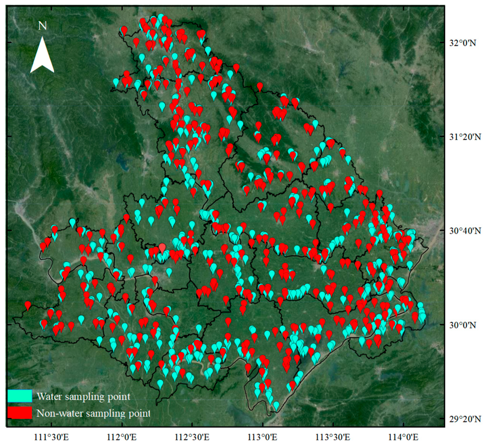
3.3. Validation of Water Body Extraction Data

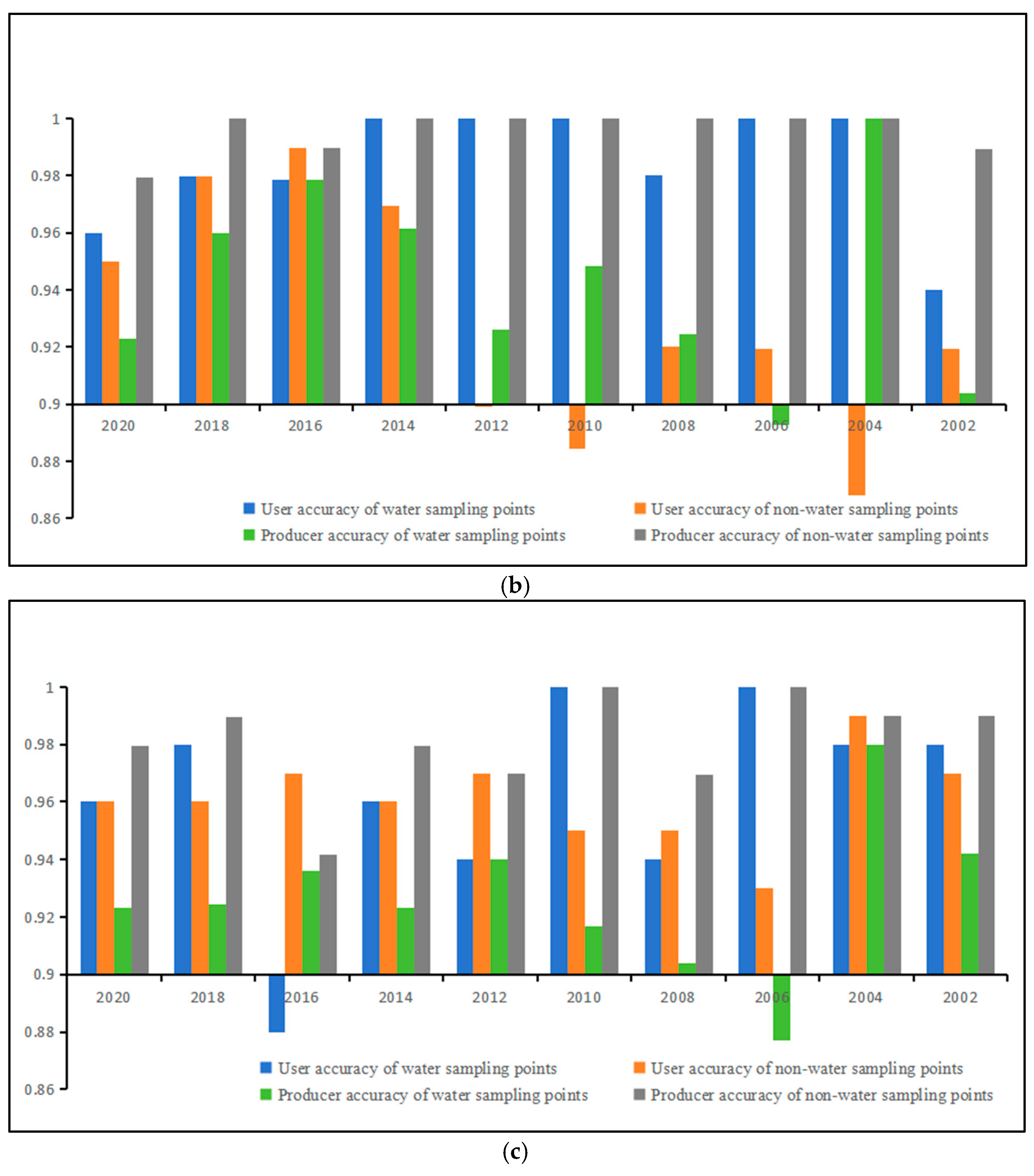
3.3.1. Accuracy Evaluation Metrics

The algorithm accuracy verification adopts the confusion matrix verification method, which lists the correspondence between the algorithm classification results and the reference data, including the number of correctly classified and misclassified pixels. Accuracy, recall, F1 score, and other indicators can be calculated to evaluate the accuracy of the algorithm [37]. We used overall accuracy (OA), Kappa coefficient, producer accuracy, and user accuracy evaluation algorithms to characterize the accuracy of the extracted water bodies. As shown in Formula (4), OA refers to the ratio of the number of correctly classified class samples to the total number of class samples. As shown in Formula (5), the Kappa coefficient represents the proportion of error reduction between correct classification and completely random classification. Producer accuracy represents the probability that the ground truth reference data of this category will be correctly classified In this classification. The user accuracy represents the ratio of correctly classified checkpoints on the classification map that fall into that category in this classification [38].
O A = i = 1 2 X i i X i + + X + i
K a p p a = O v e r a l l   a c c u r a c y E x p e c t e d   a c c u r a c y 1 E x p e c t e d   a c c u r a c y = N i = 1 n X i i i = 1 n ( X i + × X + i ) N 2 i = 1 n ( X i + × X + i )
In the formula, n represents the category, N represents the total number of categories (this refers to the number of test points), X i i represents the diagonal elements of the error matrix, X i + represents the total number of columns for the category, and X + i represents the total number of rows for the category.

3.3.2. Accuracy Evaluation

To verify the accuracy of the algorithm, water bodies extracted using methods such as the JRC dataset, the Synthetic Aperture Radar (SAR) Wetland Detection Index (SDWI) index, and Landsat 8 permanent water bodies were compared with those extracted using the Landsat 5, 7, and 8 multi-source fusion threshold method.
The JRC dataset was generated using 4,716,475 scenes collected from the Landsat 5, 7, and 8 satellites between 1984 and 2021. An expert system is used to separately classify each pixel as a water body or not. The results are organized as monthly historical dataset for the entire time period and change detection dataset for two time periods (1984–1999, 2000–2021).
SDWI is a remote sensing index used to extract water bodies. It is calculated from Sentinel-1 SAR data, which uses Vertical–Horizontal (VH) and Vertical–Vertical (VV) band data in the image to calculate SDWI values. The SDWI value represents the reflection and scattering characteristics of a water body. As Sentinel-1 was launched in 2014, data covering the whole year are only available from 2015 onwards. Application of the method to long time series of water extractions is not appropriate.
Landsat 8 permanent water bodies use Landsat 8 satellite imagery data for cloud removal, scaling, and adding different vegetation indices (NDVI, EVI, MNDWI, and Land Surface Water Index (LSWI)). Then, water bodies are extracted by calculating different water frequency formulas. Landsat 8 only used one satellite source to extract permanent water bodies, non-water bodies, and seasonal water bodies, and classified them into three categories.
Starting from 2002, 100 water points and 50 non-water points were selected every two years by corresponding year background images, which contains both Landsat 5/7/8 images and Sentinel-1/2 images. Totally, 1000 water samples and 500 non-water samples were used to evaluate the accuracy of water extraction methods. The distribution of sampling points is shown in Figure 4. The accuracy of the four methods is shown in Table 3.
The Landsat Multi-Index Relationship and Water Probability Thresholding Method has the highest OA, followed by SDWI. As the SDWI algorithm is calculated using Sentinel-1 image data, and Sentinel-1 was only launched on April 3, 2014, it can only calculate its water body from 2015 to 2021, resulting in higher average accuracy [39]. The JRC dataset and Landsat 8 permanent water bodies methods have been validated with user accuracy and production accuracy below 0.9 over one or several years, indicating time instability, as shown in Figure 5. On the other hand, the Landsat multi-satellite fusion threshold method has a minimum value of about 0.907 in user accuracy and producer accuracy, both exceeding 90% accuracy, showing high temporal accuracy in water extraction over a long time series.
Based on the accuracy obtained by the four sampling methods in Table 3, it was ultimately determined that the Landsat multi-exponential relationship and water probability threshold method exhibit high spatio-temporal stability accuracy in extracting water bodies from the Jianghan Plain. This method proves to have advantages in extracting water bodies from areas such as the Jianghan Plain.
The Landsat multi-index method can not only perform long-term spatio-temporal analysis, but also reduce the extraction error of the water index method. For land categories such as paddy fields with similar reflectance to water, this algorithm can distinguish them effectively, as shown in Figure 6a,b. However, for small linear rivers, such as artificially constructed narrow water bodies like ditches, a spatial resolution of 30 m can lead to an inability to distinguish water bodies when the river is extremely narrow, resulting in river disconnection, as shown in Figure 6c,d. This issue may lead to a deviation in the number of water bodies in the calculation area, and ArcGIS will be used for manual fusion in the future.

4. Results and Analysis

4.1. Long-Term Water Landscape Indices in Jianghan Plain

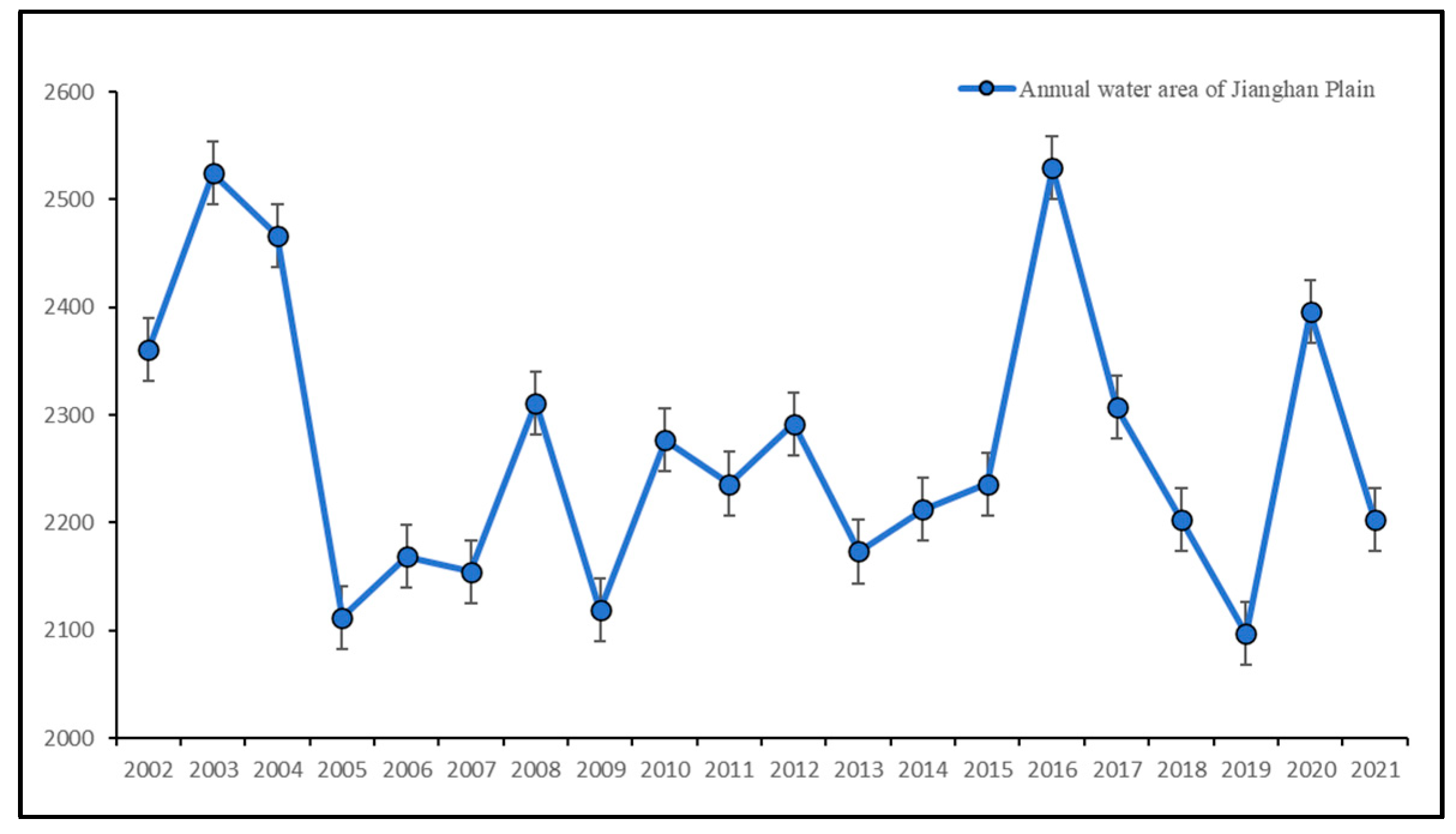
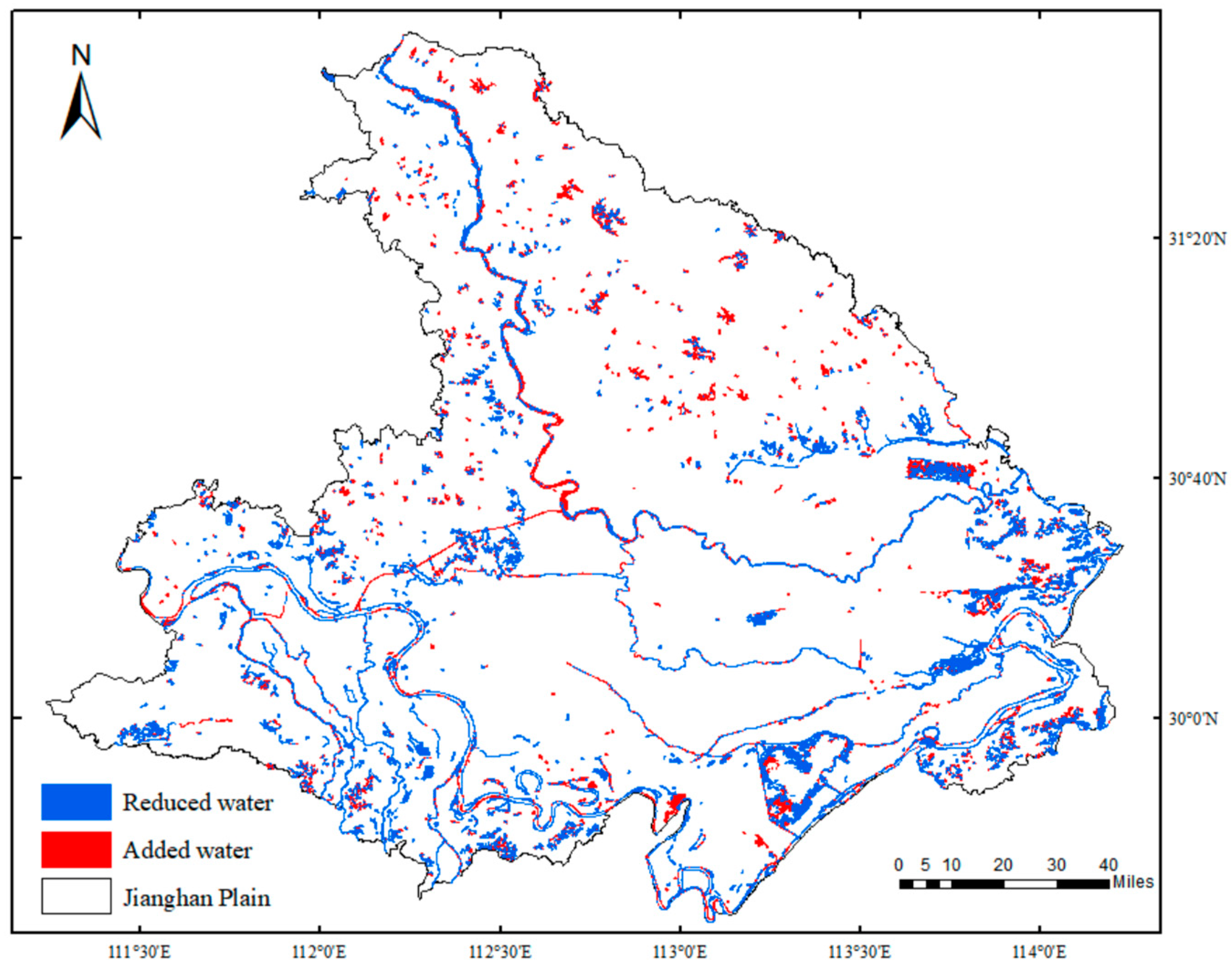
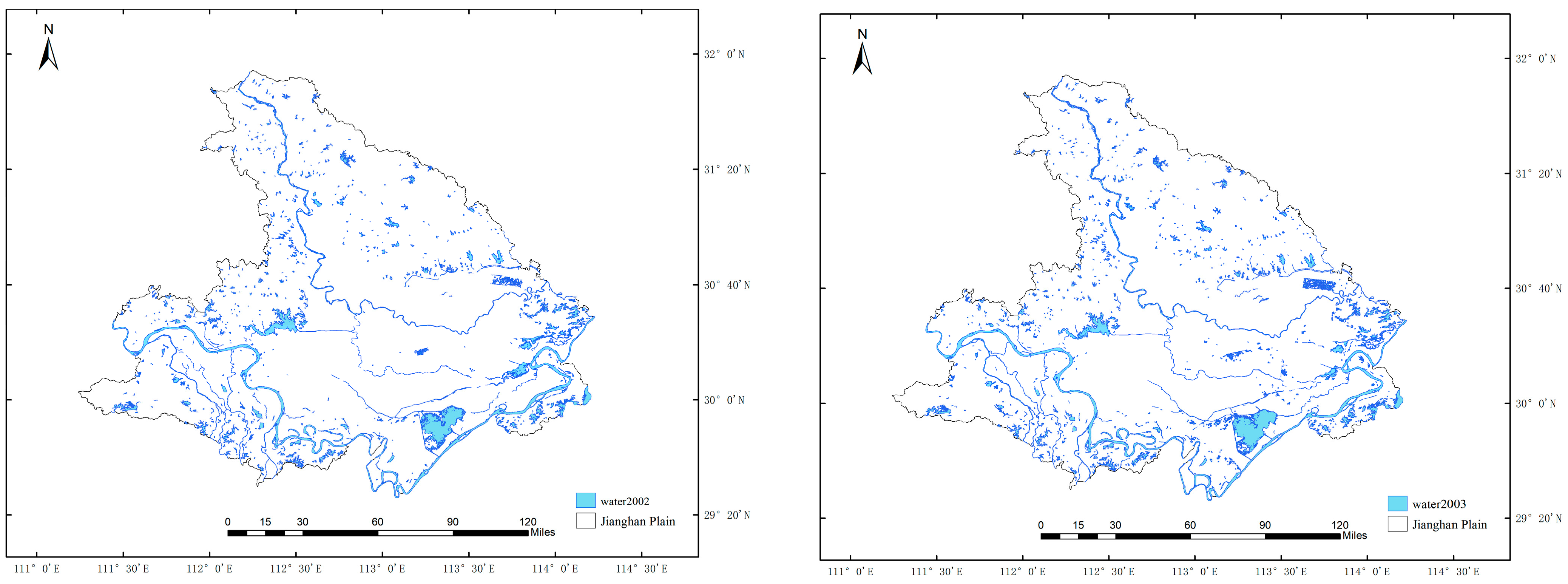
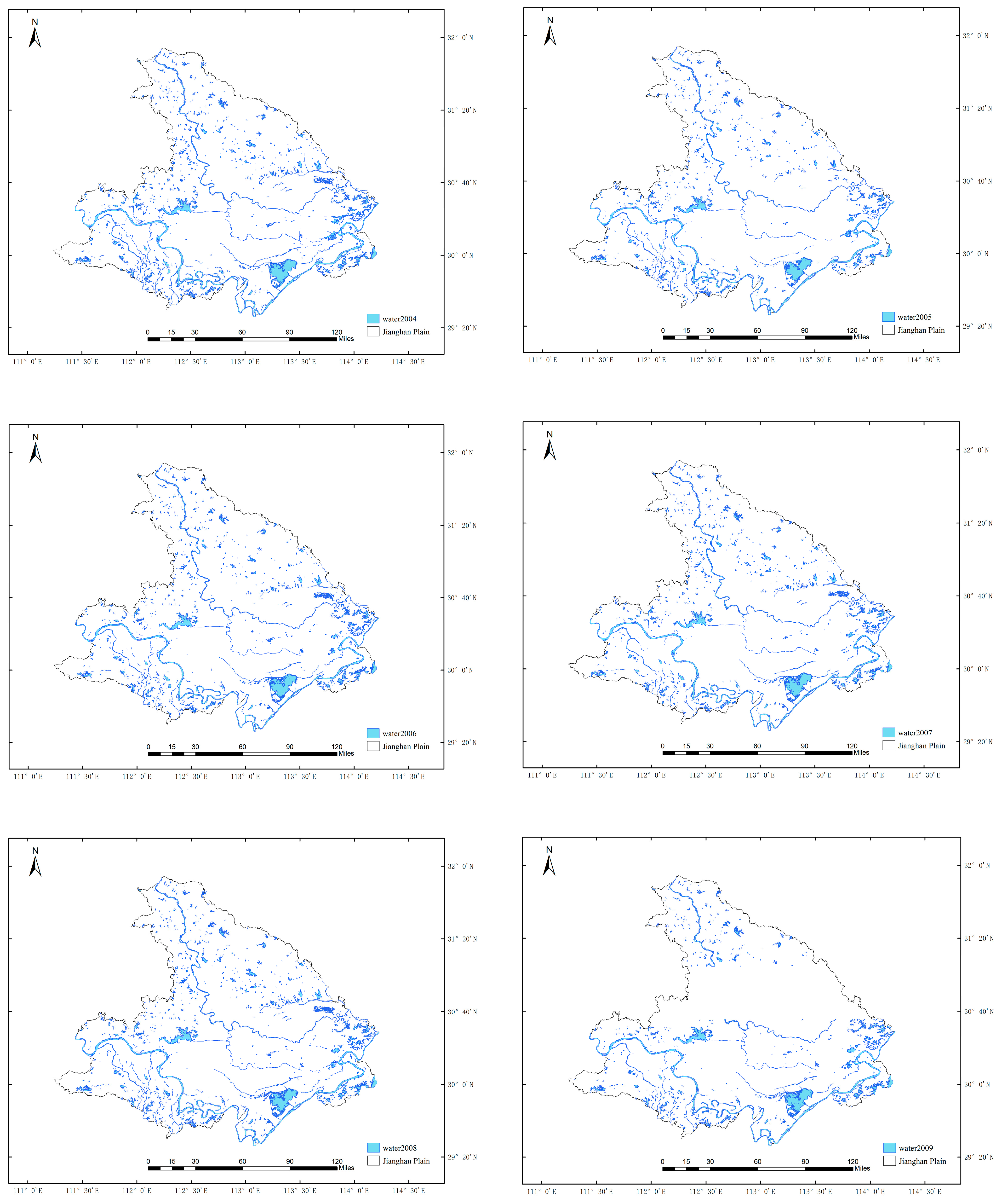
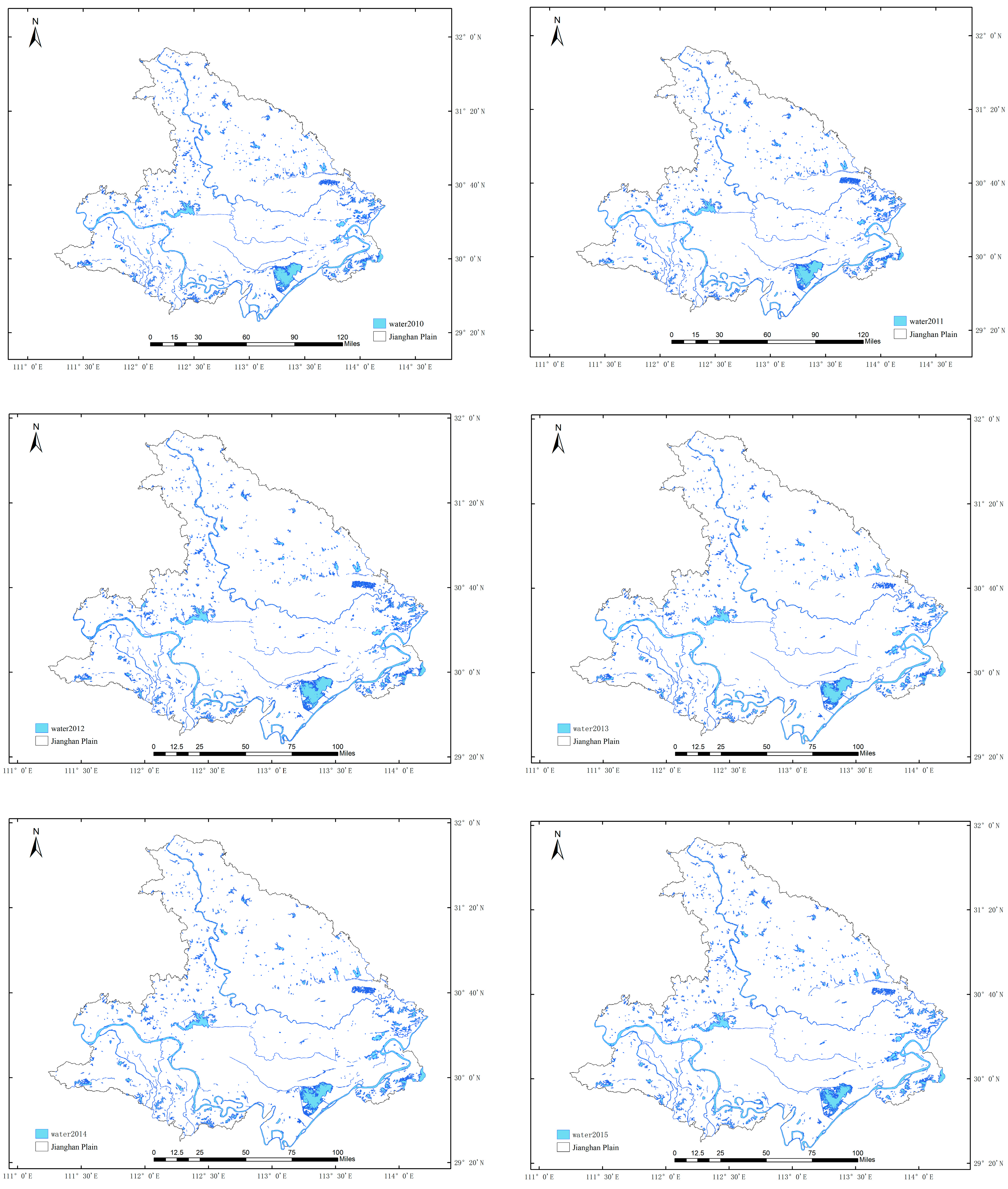
4.1.1. Spatio-Temporal Evolution Characteristics of the Water System

Figure 7 shows the water area of the Jianghan Plain from 2002 to 2021. Figure 8 shows the increase and decrease in water bodies over the 20-year period from 2002 to 2021. Figure 9 shows the distribution of water systems in the Jianghan Plain over the past 20 years. It can be seen that the overall water volume of the Jianghan Plain is abundant, with a wide range and high distribution density of water bodies. In the past 20 years, the distribution of linear water bodies has been relatively stable, while some surface water bodies (represented by lakes and reservoirs) have shown a significant trend of reduction, such as lake discharge, with an area reduction of more than half and a significant decrease in the number of surface water bodies. Liu et al. [40] also pointed out that in the past 20 years, the total amount of water resources in China has shown a decreasing trend. This may be related to social and economic activities, such as lake reclamation. However, the relative areas of Changhu and Honghu are relatively stable, making them the two largest lakes in the plain, indicating that their ecological conditions are relatively stable. The overall water area has a significantly larger range in 2016 and 2020, which is correlated with a significant increase in precipitation in these two years.

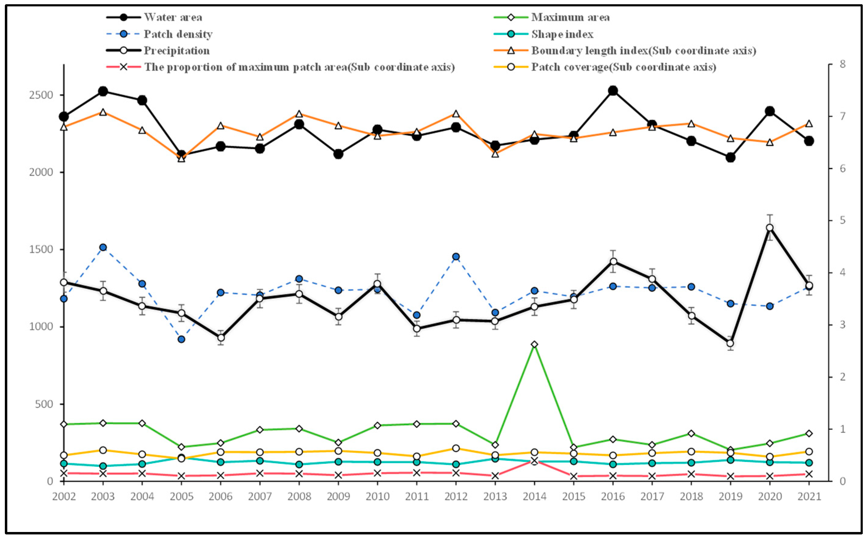
4.1.2. Temporal Characteristics of Water Landscape Indices

Figure 10 shows the temporal changes of eight landscape indices for the entire Jianghan Plain from 2002 to 2021, with the average annual precipitation depth in Hubei Province. The average precipitation depth in Hubei Province shows a fluctuating trend overall, with an average annual precipitation of about 1170.25 mm. The highest precipitation was recorded in 2020, at 1642.6 mm, followed by 2016. In contrast, 2006, 2009, 2011, and 2019 experienced relatively low precipitation, with decreases of 21.2%, 9.6%, 16.2%, and 24.3% compared to normal years, respectively. The trend of changes in water area and precipitation is relatively consistent.
According to Figure 10, it is found that the water landscape index shows fluctuating changes. In 2003, the patch coverage was significantly higher than in other years. During this time, the water area was larger, and the proportion of the largest patch was relatively small, indicating that the distribution of the water system was relatively fragmented in that year. This fragmentation could have been caused by human activities, such as filling, widening, and cofferdam, which increased the water area but also divided the water into smaller patches.
In 2009, a dry year, the water area in each region decreased while the patch coverage increased. Besides lower precipitation, it is speculated that a large amount of land was developed for agriculture or urban construction, resulting in water bodies being buried or converted for other purposes, thereby reducing the water area and causing water bodies to become fragmented. The year 2005 was also a drought year, and the analysis is similar to 2009.
In years with high precipitation, such as 2016 and 2020, the patch coverage and shape index were low, and the proportion of the largest patches and water area were high. This indicates that small and medium-sized water bodies connected together in these two years, forming regular shapes and abundant water resources. Historically, Hubei Province experienced major floods during this time. By analyzing the water landscape index, it is possible to identify flood years and drought years. However, various abnormal water landscape index situations can be attributed to human activities.
Research on the Changhu area in the Jianghan Plain. Comparing the water system differences between the drought year of 2005 and the flood year of 2016, as shown in Figure 11, it can be seen that in flood years, the Changhu area in the Jianghan Plain expands outward, and the Yangtze River central island in the lower left corner is also basically submerged.

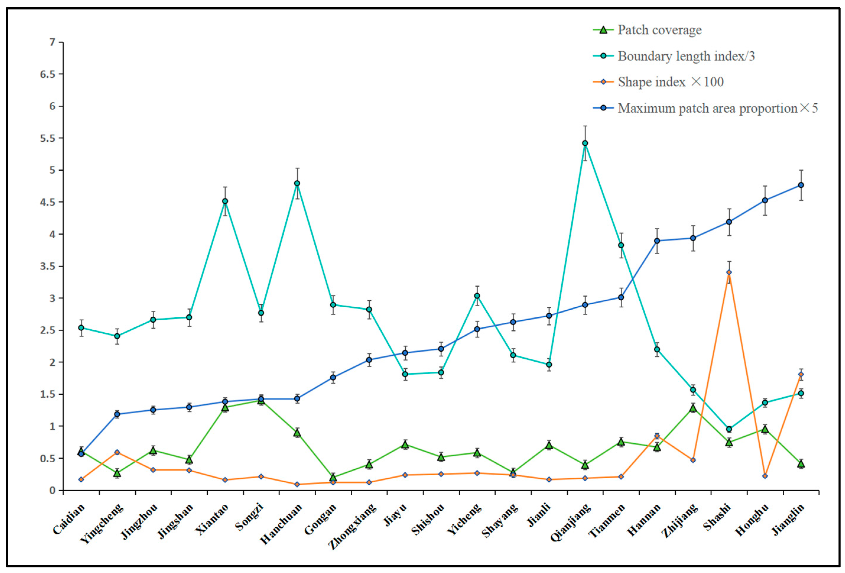
4.1.3. Spatial Distribution Characteristics of Water Landscape Index

According to Table 2, it can be seen that regions with higher shape indices have more regular and compact water bodies. The higher the boundary length index, the more complex the terrain, numerous the lakes and rivers, and fragmented the area. High patch density reflects the richness and complexity of the landscape in a geographical region and displays a more complex and fragmented spatial pattern. The proportion of maximum area reflects the importance of the largest water body in a geographical area to the entire region. Figure 12 shows the water landscape indices of various districts and counties in the Jianghan Plain in 2021, including patch coverage, boundary length index, shape index, and maximum patch area proportion. According to Figure 12, the shape index of Shashi District and Jiangling County is relatively large, while the boundary length index is relatively small; the boundary length index of Hanchuan City, Qianjiang City, and Tianmen City is relatively large, while the shape index is relatively small; the largest patch area accounts for a relatively large proportion in Hannan District, Zhijiang City, Shashi District, Jiangling County, and Honghu City; and Hanchuan City, Qianjiang City, and Tianmen City have a high density of patches. It can be concluded that regions with higher patch density and boundary length index have smaller proportions of shape index and maximum patch area.
Therefore, the water landscape index can provide rough inferences about the complexity, dispersion, and importance of patches in geographic spatial regions, which has important reference value for environmental protection, land planning, and resource management.

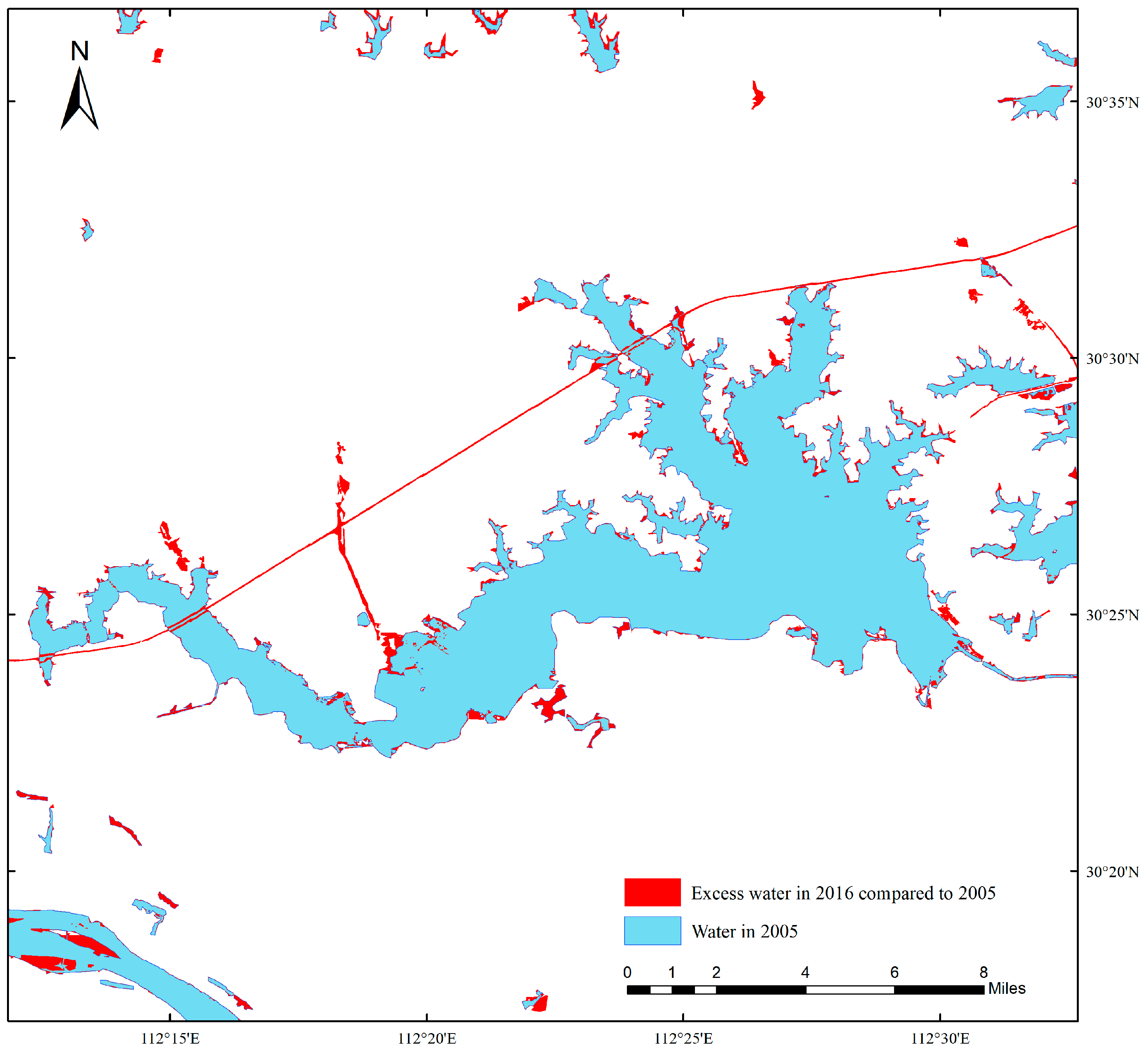
4.1.4. Analysis of Typical Area

Figure 13 shows the precipitation in Hannan District and Honghu City for the year 2015, 2016, and the multi-year average. Figure 14a,b display the distribution of water bodies and the water landscape index over a period of 20 years in Caidian District. Take Caidian District as an example: In 2016, the water area, maximum area of county water body, and maximum circumference were significantly higher than other years. According to the 2016 Wuhan Water Resources Bulletin, the precipitation in various districts of Wuhan in 2016 was generally higher than in previous years. Compared with the annual average, Huangpi District had an increase of about 40%, while the central urban area, Jiangxia District, and Xinzhou District had an increase of 50–60%. Hannan District and Dongxihu District had an increase of 60–70%, and Caidian District had an increase of about 75%. Based on the water conditions of that year, Wuhan City was affected by a super strong El Niño in 2016 and suffered from the most severe flood disaster since 1998 [41]. Wuhan City took various measures to prevent and reduce floods, such as strengthening flood embankments and dredging the main waterways of rivers. In 2016, Wuhan City achieved a decisive victory in flood prevention and control. In 2017, the water landscape index returned to normal, indicating that the measures taken have played a positive role in the restoration and protection of the water landscape. In addition, the boundary length index and patch density in Caidian District are relatively high, while the shape index and maximum patch area are relatively small, indicating that the boundaries of rivers and lakes in this area are complex and scattered, presenting fragmentation and not affecting the overall water body of the region.
Figure 14c,d show the distribution of water bodies and the water landscape index over a period of 20 years in Honghu City. Taking Honghu City as an example: like Caidian District, according to the 2016 Water Resources Bulletin of Jingzhou City, the precipitation in Honghu City increased by 35.5% compared to previous years. Honghu City has a relatively high proportion of maximum patch area, while the other three indices are relatively low. The reason is that Honghu Lake is located in this area, and it plays an extremely important role in the water system of Honghu City. The boundary of Honghu Lake is uneven, resulting in a relatively low shape index of Honghu City. In fact, the water system of Honghu City mainly comes from Honghu Lake, with its simple terrain and fewer rivers and lakes.

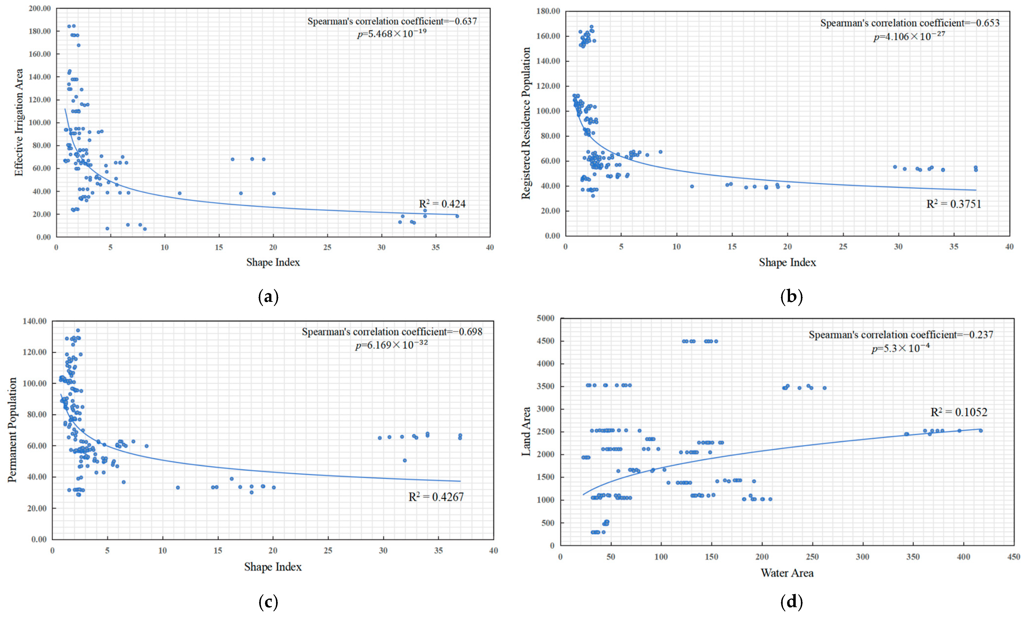
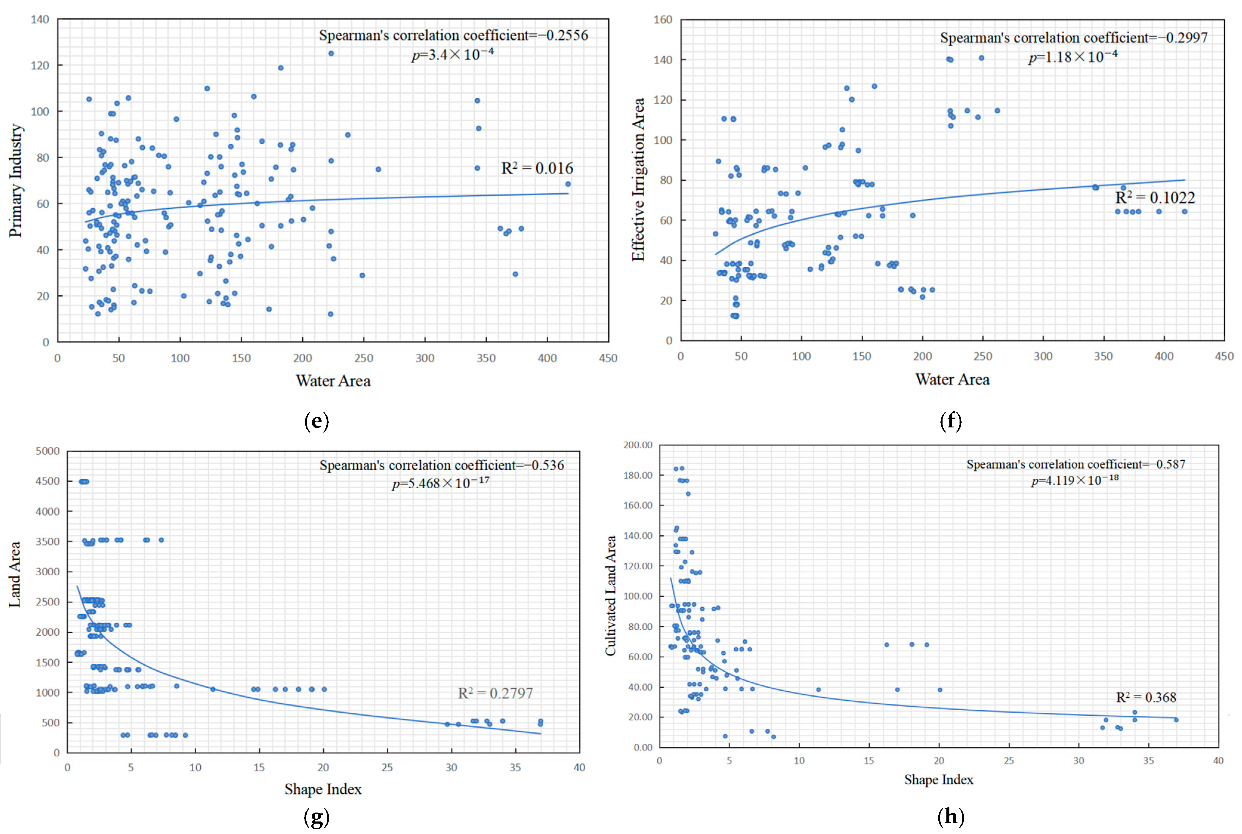
4.2. Correlation Relationships between the Water Landscape Indices and Economic Attributes

In order to understand the relationship between water systems and urban economic attributes, the Spearman correlation coefficient was selected to analyze the relationship between the various water landscape indices and urban economic attributes. The Spearman correlation coefficient measures the monotonic relationship between two sets of data, not limited to linear relationships. The Spearman correlation coefficient has good robustness to outliers and nonlinear relationships. Figure 15 shows the correlation analysis between the water body landscape index and urban economic attributes. The urban economic attribute data of Jianghan Plain in this paper is composed of cultivated land area, effective irrigation area, highway mileage, land area, registered residence population, permanent population, gross national product, gross national product of the primary industry, gross national product of the secondary industry, gross national product of the tertiary industry, and other data of 21 counties and districts in Jianghan Plain from 2012 to 2021. The water landscape index consists of total water area, total water length, number of patches, maximum water area, proportion of maximum patch area, patch coverage, boundary length index, and shape index. As shown in Figure 15, the high correlation between water landscape index and economic attributes includes shape index and effective irrigation area, shape index and permanent population, shape index, and registered residence population.
Judging the correlation between data, taking the shape index and effective irrigation area as an example, as shown in Figure 15a, assuming that the shape index is not correlated with effective irrigation area, the calculated probability value p-value is 5.468 × 10⁻¹⁹, which is far less than 0.01, indicating that the correlation coefficient is significant. Refusing the null hypothesis, that is, there is a statistically significant correlation between the shape index and effective irrigation area. At the same time, the Spearman correlation coefficient is −0.637, greater than −0.6, indicating a strong negative correlation between the two sets of data. By comparing their goodness of fit, it can be seen that the power model has a higher fitness in the relationship between shape index and effective irrigation area. Therefore, it is believed that the shape index is strongly negatively correlated with effective irrigation area. The correlation of other data is the same.
The smaller the shape landscape index, the more complex the water boundary in the area, with more branches and curves. The shape landscape index shows a strong negative power correlation with the effective irrigation area. The more complex the water body boundary, the larger the buffer zone range around it, and the larger the land area that can be irrigated. In addition, there is a strong negative power correlation between the shape landscape index and population, indicating that the smaller the shape landscape index, the higher the water fragmentation and irregularity, and the more population there is in the region. The reasons for this phenomenon can be divided into two categories: first, human activities and urbanization development have led to changes in water bodies. The cultivation of arable land, the planting of flood prevention forests, urbanization construction, and mineral development all have an impact on water bodies, resulting in lower shape indices. The second reason is that most of people’s cultivated land irrigation, domestic water, and industrial water come from the water system within their region. The dispersed layout and highly complex water bodies provide more water resources to attract population migration.
Subjectively, it is believed that the larger the land area occupied by a county, the larger the water body area it usually contains. However, in reality, the correlation between the water area and land area of each county in the Jianghan Plain is weak, as shown in Figure 15d. The reason for this is related to many factors, such as terrain, human activities and development, regional precipitation, etc. Analysis has found that there is not a strong correlation between water area, primary industry, and effective irrigation area. Under the promotion of comprehensive water environment management policies, efforts are being made to ensure the basic ecological water use of rivers and lakes and to coordinate the development of regional water systems and economy. Therefore, areas with more water systems and dispersed distribution have higher efficiency in utilizing water bodies than cities with fewer water systems and concentrated distribution.

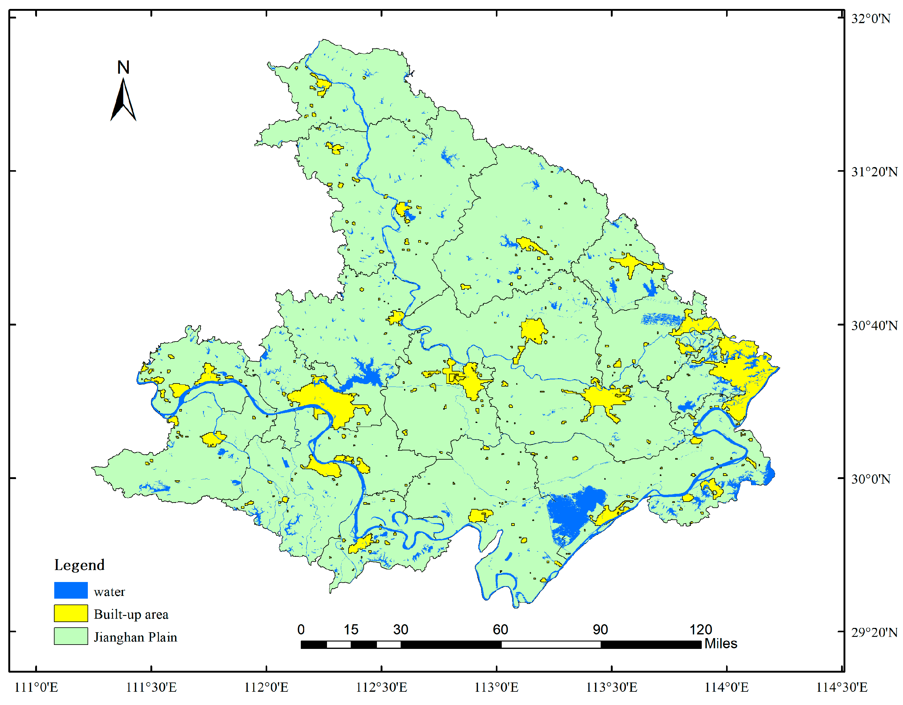
4.3. The Associative Characteristics between Water Bodies and Built-Up Areas

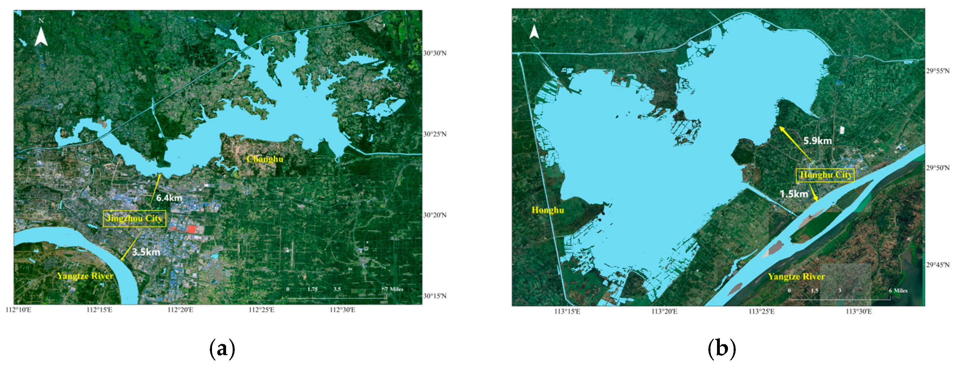
4.3.1. Analysis of Distance between Centers of Built-Up Areas and Water Bodies

Figure 16 shows the distances between the built-up areas closest to the five major water bodies, as well as the built-up area. Table 4 analyzes Figure 16 and obtains the distance from the built-up area with the highest peak area to the nearest water body. Using GEE to obtain the “build” type from DW land classification images, the data were exported to ArcGIS to calculate the closest distance between the center of the built-up area and five large rivers in the Jianghan Plain. These rivers include the Yangtze River, Han River, Dongjing River, Neijing River, and Hanbei River.
According to Table 4, the higher the scale of the river, the closer the distance between large built-up areas, and the more prosperous the city. The distribution of rivers and built-up areas are shown in Figure 17. In fact, some scholars have found a similar phenomenon in their research. Li et al. [42] found that the formation of the canal ring in the Amsterdam area played a dominant role in the establishment of urban spatial form. The Qiantang River, West Lake, and the Beijing Hangzhou Canal also played different dominant roles in the urban form of Hangzhou at different times.
Most of the built-up areas are distributed along the river and on the concave banks of the river. Rivers experience concave bank erosion and convex bank accumulation at their bends. Convex banks are sedimentary banks that are conducive to sediment accumulation and can form deep and fertile soil, facilitating the development of agriculture [43]. Concave shores can establish ports for transportation. With the development of the economy since modern times, the development of the shipping logistics industry has attracted a large number of people and logistics to gather and transfer here, making it an ideal environment for urban logistics transfer.

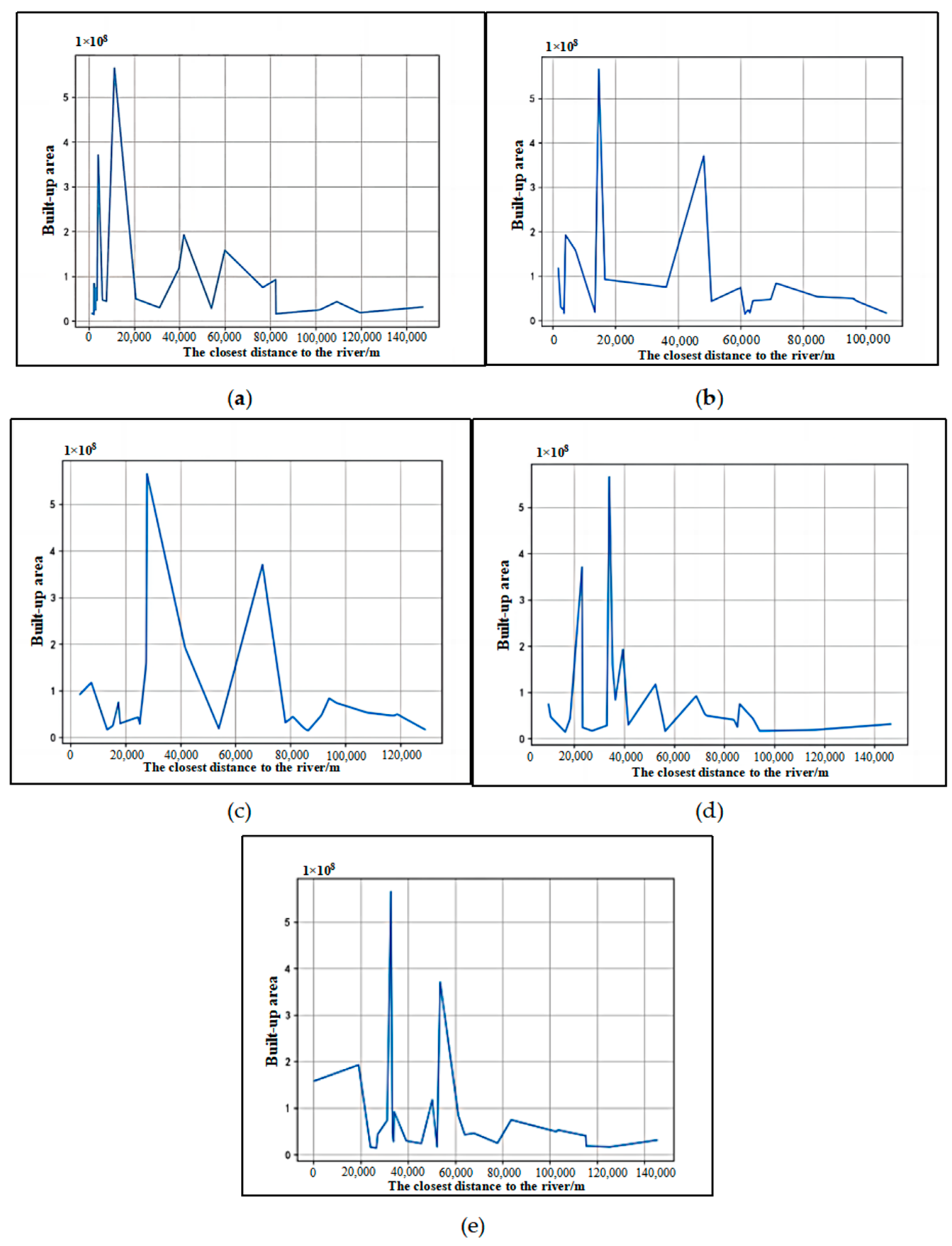
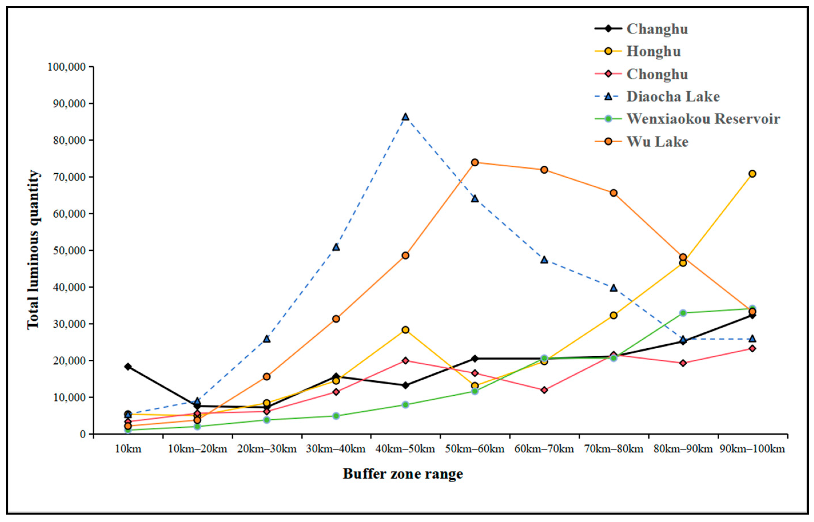
4.3.2. Analysis of Built-Up Areas within the Buffer Zone of Water Bodies

Figure 18 shows the total luminous quantity in different buffer zones of large lakes in the Jianghan Plain. As shown in Figure 18, the small peaks in the built-up areas of lakes are mostly distributed within a range of 30–60 km. In recent years, people have gradually realized the importance of an ecological environment, and static lakes are more susceptible to pollution than dynamic rivers. Once affected by pollution, the difficulty of restoration may be greater. Therefore, most urban centers are not very close to lakes. Honghu and Changhu are the two largest lakes in the Jianghan Plain. Figure 19a shows the distances from Jingzhou City to the Yangtze River and Changhu. Figure 19b displays the distances from Honghu City to the Yangtze River and Honghu. Taking Honghu as an example, Honghu is located to the west of the central urban area of Honghu. Its small peaks are mostly contributed by the central urban area of Honghu, and most of the surrounding areas are cultivated land. The central urban area of Honghu is located along the Yangtze River, far from the lake, and most cities are built along the river (see Figure 19).

5. Conclusions

This article is based on the JavaScript interactive operating environment on the GEE platform. The Landsat 5, 7, and 8 SR datasets were selected, and the low cloud cover images from 2002 to 2021 were used for processing, analysis, and calculation. The accuracy was verified by collecting sample points. The output results were studied and plotted on the ArcGIS platform, and various water landscape indices were calculated to reveal the relationship between water space and urban economic attributes in the Jianghan Plain. Combined with DW built-up area data, the connection between water systems and urban planning is judged. The following conclusions are drawn:
(1)
The complexity of water bodies is strongly negatively correlated with population and effective irrigation area, indicating that changes in water systems will significantly affect socio-economic activities.
(2)
The higher the level and scale of the river, the closer the built-up area is to the river and the larger the area, indicating that the water system affects the planning and construction of the city.
(3)
Cities in Jianghan Plain are mostly built along rivers and are mostly distributed on concave banks.
The algorithm in this article provides important arithmetic support for water extraction in the Jianghan Plain, but there are still some limitations. Our research results are only applicable to plain areas with relatively flat and open terrain and humid climate, and further research and verification are needed for their applicability to other regions. In addition, after visual inspection, some rivers are extremely small and cannot be extracted due to insufficient spatial resolution. Meanwhile, due to the use of long-term annual Landsat images, the extraction and accuracy verification of water bodies take a relatively long time, and there is still room for improvement in both automated and semi-automated water body extraction algorithm schemes. To obtain more accurate results and analyze the relationship between water and economy, it is possible to further combine information from hydrological observation stations to study the extraction of narrow rivers and the estimation of water levels, providing a foundation for future research.
The research results of this article emphasize the importance of water bodies in urban planning, providing new insights into the relationship between water body area and urban economic attributes. It has important reference value for urban planners and decision-makers in protecting water resources, rational planning of land use, and promoting sustainable urban development. By utilizing the obtained water landscape index, future water change trends such as water quality changes and water level fluctuations, correlation analysis between water systems and other newly added urban economic attributes, water resource supply and demand analysis, and land classification analysis at large water turning points can be analyzed, providing support for the sustainable development of cities and the protection and management of water resources.

Author Contributions

Conceptualization, W.Z.; methodology, F.D. and J.H.; software, F.D.; validation, L.M.; formal analysis, L.L.; investigation, F.D. and J.H.; resources, F.D. and W.Z.; data curation, F.D., J.H., L.M., L.L. and W.Z.; writing—original draft preparation, F.D. and W.Z.; writing—review and editing, F.D., J.H., L.M., L.L. and W.Z.; visualization, F.D.; supervision, W.Z.; funding acquisition, W.Z. All authors have read and agreed to the published version of the manuscript.

Funding

This work was supported by the National Key R&D Program of China under Grant No.2021YFB3900603.

Data Availability Statement

Restrictions apply to the datasets. The data partially belong to a private entity.

Acknowledgments

We appreciate the data provider for the above data. We would also like to thank the Wuhan University for managing the campaign.

Conflicts of Interest

The authors declare no conflicts of interest.

Abbreviations

GEEGoogle Earth Engine
OAoverall accuracy
JRCJoint Research Centre
EREcological resilience
SRsurface reflectance
DWDynamic World
NDWINormalized Difference Water Index
MNDWIModified Normalized Difference Water Index
MBWIMulti-Band Water Index
AWEIAutomatic Water Extraction Index
NDVINormalized Difference Vegetation Index
EVIEnhanced Vegetation Index
SARSynthetic Aperture Radar
SDWISAR Wetland Detection Index
VHVertical–Horizontal
VV Vertical–Vertical
LSWILand Surface Water Index

References

  1. He, F.; Lu, P.Y.; Yin, J. Spatial Equilibrium Evaluation and Spatial Correlation Analysis of Water Resources in China. Water Resour. Prot. 2023, 39, 148–155. [Google Scholar]
  2. Chang, T.; Li, J.; Guo, X. The spatial temporal characteristics and driving force analysis of water area landscape pattern changes on the Jianghan Plain. Adv. Water Sci. 2023, 34, 21–32. [Google Scholar]
  3. Su, L.F.; Li, Z.X.; Gao, F. A review of research on remote sensing image water extraction. Land Resour. Remote Sens. 2021, 33, 9–19. [Google Scholar]
  4. Yang, C.J.; Zhou, C.H. Extracting Residential Areas on the TM Imagery. J. Remote Sens. 2000. [Google Scholar] [CrossRef]
  5. Cui, Q.; Wang, J.; Wang, M. Vector constrained object-oriented high-resolution remote sensing image water extraction. Remote Sens. Inf. 2018, 33, 115–121. [Google Scholar]
  6. Tang, D.K.; Wang, F.; Wang, H.Q. A single polarization SAR data flood water detection method based on Markov segmentation. J. Electron. Inf. Technol. 2019, 41, 619–625. [Google Scholar]
  7. Li, X.G. Research on Water Body Recognition Based on Deep Learning; Harbin Normal University: Harbin, China, 2020. [Google Scholar]
  8. Franke, C.; Schweikart, J. Mental representation of landmarks on maps: Investigating cartographic visualization methods with eye tracking technology. Spat. Cogn. Comput. 2017, 17, 20–38. [Google Scholar] [CrossRef]
  9. Legleiter, C.J. A geostatistical framework for quantifying the reach-scale spatial structure of river morphology: 1. Variogram models, related metrics, and relation to channel form. Geomorphology 2014, 205, 65–84. [Google Scholar] [CrossRef]
  10. Nguyen, C.; Daly, E.; Pauwels, V.R.N. A dynamic connectivity metric for complex river wetlands. J. Hydrol. 2021, 603, 127163. [Google Scholar] [CrossRef]
  11. Horton, R.E. Erosional development of streams and their drainage basins; hydrophysical approach to quantitative morphology. Geol. Soc. Am. Bull. 1945, 56, 275–370. [Google Scholar] [CrossRef]
  12. Vassoney, E.; Mochet, A.M.; Bozzo, M. Definition of an indicator assessing the impact of a dam on the downstream river landscape. Ecol. Indic. 2021, 129, 107941. [Google Scholar] [CrossRef]
  13. Fang, G.; Yan, M.; Dai, L. Improved indicators of hydrological alteration for quantifying the dam-induced impacts on flow regimes in small and medium-sized rivers. Sci. Total Environ. 2023, 867, 161499. [Google Scholar] [CrossRef]
  14. Bosch, M.; Jaligot, R.; Chenal, J. Spatiotemporal patterns of urbanization in three Swiss urban agglomerations: Insights from landscape metrics, growth modes and fractal analysis. Landsc. Ecol. 2020, 35, 879–891. [Google Scholar] [CrossRef]
  15. Zhu, Z.; Liu, B.; Wang, H. Analysis of the spatiotemporal changes in watershed landscape pattern and its influencing factors in rapidly urbanizing areas using satellite data. Remote Sens. 2021, 13, 1168. [Google Scholar] [CrossRef]
  16. Zhai, H.; Lv, C.; Liu, W. Understanding spatio-temporal patterns of land use/land cover change under urbanization in Wuhan, China, 2000–2019. Remote Sens. 2021, 13, 3331. [Google Scholar] [CrossRef]
  17. Fu, F.; Deng, S.; Wu, D. Research on the spatiotemporal evolution of land use landscape pattern in a county area based on CA-Markov model. Sustain. Cities Soc. 2022, 80, 103760. [Google Scholar] [CrossRef]
  18. Chen, D.; Zhang, F.; Jim, C.Y. Spatio-temporal evolution of landscape patterns in an oasis city. Environ. Sci. Pollut. Res. 2023, 30, 3872–3886. [Google Scholar] [CrossRef]
  19. Huang, L.; Zhang, W.; Jiang, C.; Fan, X. Ecological footprint method in water resources assessment. Acta Ecol. Sin. 2008, 28, 1279–1286. Available online: http://www.ecologica.cn/stxb/ch/reader/create_pdf.aspx?file_no=1000-0933200803-1279-08&flag=1&journal_id=stxb&year_id=2008 (accessed on 6 May 2024).
  20. Wang, S.; Li, Z.; Long, Y. Impacts of urbanization on the spatiotemporal evolution of ecological resilience in the Plateau Lake Area in Central Yunnan, China. Ecol. Indic. 2024, 160, 111836. [Google Scholar] [CrossRef]
  21. Ren, W.; Zhang, X.; Peng, H. Evaluation of temporal and spatial changes in ecological environmental quality on Jianghan Plain from 1990 to 2021. Front. Environ. Sci. 2022, 10, 884440. [Google Scholar] [CrossRef]
  22. Chen, P.; Chen, X.F.; Li, S.L. Analysis of spatiotemporal variation of water quality in the Jianghan Plain from 2016 to 2021[J/OL]. J. Guangxi Norm. Univ. 2024, 1–8. [Google Scholar] [CrossRef]
  23. Sing, T.; Li, J.Q.; Guo, X.N. Analysis of spatiotemporal evolution characteristics and driving factors of water spatial pattern in the Jianghan Plain. Prog. Water Sci. 2023, 34, 21–32. [Google Scholar]
  24. Hou, X.J. Research on the Spatiotemporal Dynamics of Suspended Sediment Concentration in Large Lakes and Reservoirs in the Middle and Lower Reaches of the Yangtze River Based on Remote Sensing and Its Relationship with Wetland Vegetation Cover; Wuhan University: Wuhan, China, 2020. [Google Scholar]
  25. Gong, R. The first satellite of the Copernicus program in Europe, Sentinel-1A, has been put into orbit. Int. Space 2014, 5, 41–44. [Google Scholar]
  26. Yin, X.G.; Jiang, W.G.; Ling, Z.Y.; Wang, X.Y.; Deng, Y.W. Evaluation and fusion of global 10 m land cover data in first batch of Chinese wetland cities. J. Remote Sens. 2023, 27, 1334–1347. [Google Scholar]
  27. Pekel, J.F.; Cottam, A.; Gorelick, N. High-resolution mapping of global surface water and its long-term changes. Nature 2016, 540, 418–422. [Google Scholar] [CrossRef]
  28. Zhu, M.S. Research on Land Use Change and Ecological Effects in the Lower Yellow River Region Based on GEE; Shandong Jianzhu University: Jinan, China, 2022. [Google Scholar]
  29. Guo, T.W.; Huang, H.L.; Sun, X.B. Thin cloud detection and removal in multispectral images of Environment 2 satellite. J. Atmos. Environ. Opt. 2023, 18, 383. [Google Scholar]
  30. Mo, J.Q.; Tang, X.M.; Li, G.Y. Research on Cloud Detection and Related Algorithms of Laser Altimeter Satellite ICESat-2. Prog. Laser Optoelectron. 2020, 57, 240–248. [Google Scholar]
  31. Wu, L.; Chen, Y.; Zhang, G. Integrating the JRC monthly water history dataset and geostatistical analysis approach to quantify surface hydrological connectivity dynamics in an Ungauged multi-lake system. Water 2021, 13, 497. [Google Scholar] [CrossRef]
  32. Brown, C.F.; Brumby, S.P.; Guzder-Williams, B. Dynamic World, Near real-time global 10 m land use land cover mapping. Sci. Data 2022, 9, 251. [Google Scholar]
  33. Claverie, M.; Vermote, E.F.; Franch, B. Evaluation of the Landsat-5 TM and Landsat-7 ETM+ surface reflectance products. Remote Sens. Environ. 2015, 169, 390–403. [Google Scholar] [CrossRef]
  34. Li, L.; Su, H.; Du, Q. A novel surface water index using local background information for long term and large-scale Landsat images. ISPRS J. Photogramm. Remote Sens. 2021, 172, 59–78. [Google Scholar] [CrossRef]
  35. Huang, S.; Tang, L.; Hupy, J.P. A commentary review on the use of normalized difference vegetation index (NDVI) in the era of popular remote sensing. J. For. Res. 2021, 32, 1–6. [Google Scholar] [CrossRef]
  36. Son, N.T.; Chen, C.F.; Chen, C.R. A comparative analysis of multitemporal MODIS EVI and NDVI data for large-scale rice yield estimation. Agric. For. Meteorol. 2014, 197, 52–64. [Google Scholar] [CrossRef]
  37. Peng, Z.H.; Tan, X. The Application of Parallel Improved Naive Bayesian Algorithm in Chinese Text Classification. Sci. Technol. Innov. 2020, 26, 176–178. [Google Scholar]
  38. Ning, X.G.; Chang, W.T.; Wang, H. Extraction of information on marshes and wetlands in the Heilongjiang River Basin using a combination of GEE and multi-source remote sensing data. J. Remote Sens. 2022, 26, 386–396. [Google Scholar]
  39. Liu, Y.; Li, L.H.; Yang, J.M.; Chen, X.; Zhang, R. Snow depth inversion based on D-InSAR method. Remote Sens. 2018, 22, 802–809. [Google Scholar] [CrossRef]
  40. Zhang, L.P.; Xia, J.; Hu, Z.F. Analysis of China’s Water Resources Status and Water Resources Security Issues. Resour. Environ. Yangtze River Basin 2009, 18, 116–120. [Google Scholar]
  41. Zhang, J.Y.; Wang, Y.T.; Liu, C.S. Special Article: Discussion on Urban Floods and Prevention Standards in China. J. Hydroelectr. Power 2017, 36, 1–6. [Google Scholar]
  42. Li, J. Comparative Analysis of the Impact of Water Systems on Urban Spatial Form: A Case Study of Amsterdam and Hangzhou. Green Technol. 2018, 7, 40–43. [Google Scholar]
  43. Wang, Z.Z.; Jia, W.Y.; Feng, W.Y. Investigation on the Relationship between County level Administrative Center Urban Areas and Rivers in Anhui Province. J. Taiyuan Norm. Univ. Nat. Sci. Ed. 2016, 15, 72–75. [Google Scholar]
Figure 1. Schematic map of Jianghan Plain.
Remotesensing 16 02770 g001
Figure 2. Algorithm flow chart.
Remotesensing 16 02770 g002
Figure 3. Water images obtained with different thresholds. (a) The water system range of Jianghan Plain when the threshold is 1. (b) The water system range of Jianghan Plain when the threshold is 0.4.
Remotesensing 16 02770 g003
Figure 4. Sample point display.
Remotesensing 16 02770 g004
Figure 5. Comparison of 10-year water extraction accuracy among three methods (excluding SDWI Index). (a) Landsat Multi-Index Relationship and Water Probability Thresholding Method. (b) JRC Dataset. (c) Landsat 8 Forever.
Remotesensing 16 02770 g005aRemotesensing 16 02770 g005b
Figure 6. Sources of error in water body extraction results. (a) Original image. (b) Range of incorrect extraction of water bodies in 2021. (c) Original image. (d) Scope of narrow water extraction in 2021.
Remotesensing 16 02770 g006
Figure 7. Water area of the Jianghan Plain from 2002 to 2021.
Remotesensing 16 02770 g007
Figure 8. Comparison of water system changes in Jianghan Plain between 2002 and 2021.
Remotesensing 16 02770 g008
Figure 9. Water system of the Jianghan Plain from 2002 to 2021.
Remotesensing 16 02770 g009aRemotesensing 16 02770 g009bRemotesensing 16 02770 g009cRemotesensing 16 02770 g009d
Figure 10. Overall water body landscape index of the Jianghan Plain region from 2002 to 2021.
Remotesensing 16 02770 g010
Figure 11. Excess water bodies in 2016 compared to 2005.
Remotesensing 16 02770 g011
Figure 12. Water landscape index in the Jianghan Plain region in 2021.
Remotesensing 16 02770 g012
Figure 13. The precipitation in Hannan District and Honghu City.
Remotesensing 16 02770 g013
Figure 14. Water system of Caidian District and Honghu City. (a) Distribution of water systems in Caidian District. (b) Caidian District Water Landscape Index. (c) Distribution of water systems in Honghu City. (d) Honghu City Water Landscape Index.
Remotesensing 16 02770 g014
Figure 15. Scatter plot of urban economic attributes and water body landscape index. (a) Correlation Analysis between Shape Index and Effective Irrigation Area. (b) Correlation Analysis between Shape Indes and Registered Residence Population. (c) Correlation Analysis between Shape Index and Permanent Population. (d) Correlation Analysis between Water Area and Land Area. (e) Correlation Analysis between Water Area and Primary Industry. (f) Correlation Analysis between Water Area andEffective lrrigation Area. (g) Correlation Analysis between Shape Index and Land Area. (h) Correlation Analysis between Shape Index and Cultivated Land Area.
Remotesensing 16 02770 g015aRemotesensing 16 02770 g015b
Figure 16. Relationship between distance to major rivers and area of built-up areas. (a) the closest distance to the Yangtze River. (b)the nearest distance to the Han River. (c) the closest distance to the Hanbei River. (d) the closest distance to the Nejing River. (e) the closest distance to the Dongjing Rivel.
Remotesensing 16 02770 g016
Figure 17. The spatial distribution of water system and built-up areas in Jianghan Plain.
Remotesensing 16 02770 g017
Figure 18. The area of urban development near large lakes.
Remotesensing 16 02770 g018
Figure 19. The distribution of the distance between Changhu and Honghu and the city center: (a) the distance between Jingzhou City and the Yangtze River and Changhu; (b) the distance between Honghu City and the Yangtze River and Honghu.
Remotesensing 16 02770 g019
Table 1. Explanation of data sources.
DataSourceData TypeSpatial ResolutionSource Link
Administrative Divisions in the Jianghan PlainOpenStreetMapVector data-hubei|OpenStreetMap (accessed on 1 December 2023)
City Economic Attributes Data of Jianghan PlainHubei Provincial Bureau of StatisticsTabular data-http://tjj.hubei.gov.cn/tjsj/sjkscx/tjnj/gsztj/whs/ (accessed on 15 December 2023)
Landsat series Surface Reflectance Data SetUnited States Geological SurveyRaster data30 mEarth Engine Data Catalog|Google for Developers (accessed on 7 January 2024)
Sentinel Satellite Image Data SetEuropean Space AgencyRaster data30 mEarth Engine Data Catalog|Google for Developers (accessed on 6 March 2024)
Dynamic World (DW) Near Real-Time Land Use and Land Cover Data SetGoogleRaster data10 mhttps://developers.google.com/earth-engine/datasets/catalog/GOOGLE_DYNAMICWORLD_V1 (accessed on 1 April 2024)
Joint Research Centre (JRC) Monthly Water History Data SetJRC of the European UnionRaster data30 mhttps://developers.google.com/earth-engine/datasets/catalog/JRC_GSW1_4_MonthlyHistory (accessed on 14 March 2024)
Table 2. Calculation formulas for water landscape indices.
Water Landscape IndicesEnglish AbbreviationFormulaTypeSelection Criteria
Water areaArea-(1) Spatial distribution of water systemsUsed to evaluate the water resource status within the watershed, which is beneficial for flood risk assessment and flood simulation model construction
Water LengthTE-Reflect the distribution and connectivity of water bodies in geographical space, as well as the distribution of different types and forms of water bodies
QuantityNP-Reflecting the distribution and spatial pattern of water bodies, measuring the degree of fragmentation of water bodies
Maximum areaLP-(2) Ecological service capacity of water systemsMeasuring the ecological function of water bodies, larger water areas provide more habitats and ecological services
The proportion of maximum patch areaLPILP/AreaEvaluate the relative importance of the largest patch in the entire landscape
Patch coveragePDNP/Area(3) Landscape complexity of water systemsAlso known as landscape fragmentation, high patch density reflects the richness and complexity of the geographical region’s landscape, and displays a more complex and fragmented spatial pattern
Boundary length indexBLITE/AreaThe high boundary length index reflects the presence of numerous isolated or dispersed patches in a geographic region
Shape indexLSI(4π × Area)/(TE2)The high shape index reflects the regular shape of geographical patches, without obvious bumps or branches
Table 3. Mean accuracy comparison of four methods from 2002–2021.
AlgorithmOAKappaClassUser AccuracyProducer’s Accuracy
Landsat Multi-Index Relationship and Water Probability Thresholding Method-Mean0.9723 0.938 Non-Water0.988 0.935
Water0.964 0.994
JRC Dataset-Mean0.9536 0.902 Non-Water0.985 0.942
Water0.937 0.996
SDWI Index-Mean0.9722 0.937 Non-Water0.957 0.960
Water0.980 0.969
Landsat 8 Forever-Mean0.9614 0.914 Non-Water0.962 0.927
Water0.961 0.981
Table 4. The nearest distance to major rivers from the center of built-up areas.
RiverDistance from the Center of Major Built-Up Areas to the Nearest River in KilometersNote
Yangtze River4 km, 10 km, 41 kmMain stream
Dongjing River30 km, 50–60 kmHan River tributary
Neijing River22 km, 34 kmYangtze River tributary
Hanbei River30 km, 70 kmHan River tributary
Han River10–20 km, 40–50 kmYangtze River tributary
Disclaimer/Publisher’s Note: The statements, opinions and data contained in all publications are solely those of the individual author(s) and contributor(s) and not of MDPI and/or the editor(s). MDPI and/or the editor(s) disclaim responsibility for any injury to people or property resulting from any ideas, methods, instructions or products referred to in the content.

