MBT-UNet: Multi-Branch Transform Combined with UNet for Semantic Segmentation of Remote Sensing Images

Abstract

Remote sensing (RS) images play an indispensable role in many key fields such as environmental monitoring, precision agriculture, and urban resource management. Traditional deep convolutional neural networks have the problem of limited receptive fields. To address this problem, this paper introduces a hybrid network model that combines the advantages of CNN and Transformer, called MBT-UNet. First, a multi-branch encoder design based on the pyramid vision transformer (PVT) is proposed to effectively capture multi-scale feature information; second, an efficient feature fusion module (FFM) is proposed to optimize the collaboration and integration of features at different scales; finally, in the decoder stage, a multi-scale upsampling module (MSUM) is proposed to further refine the segmentation results and enhance segmentation accuracy. We conduct experiments on the ISPRS Vaihingen dataset, the Potsdam dataset, the LoveDA dataset, and the UAVid dataset. Experimental results show that MBT-UNet surpasses state-of-the-art algorithms in key performance indicators, confirming its superior performance in high-precision remote sensing image segmentation tasks.

1. Introduction

Remote sensing images are images of the earth’s surface obtained from long distances, and are used for environmental monitoring [1,2], urban planning [3,4], agriculture [5,6], forestry [7,8], geological exploration [9,10], oceanography [11,12] and disaster management [13,14] and many other fields are crucial. Semantic segmentation technology plays a very key role in this process. By accurately classifying each pixel in an RS image, it is segmented into regions with specific meaning. Semantic segmentation not only greatly improves the automation and accuracy of data processing, but also makes multi-scale analysis from macro to micro possible. The research on semantic segmentation of RS images begins with simple image processing technology. Early methods, such as threshold segmentation [15], region growing [16] and edge detection [17], etc., relied on the basic characteristics of images to identify and classify ground objects. These methods are relatively effective when processing low-complexity RS images, but their performance is often limited when facing high-resolution and high-complexity modern RS images. With the advancement of machine learning methods, especially the introduction of algorithms like support vector machine (SVM) [18], conditional random field [19,20,21] and random forest [22], the performance of RS image segmentation has been improved. These methods improve the accuracy of segmentation by learning the mapping relationship between image features and feature categories. However, these approaches still depend on manually extracted features, and their performance is constrained by the effectiveness of feature extraction.

The emergence of deep learning technology has brought revolutionary changes to the semantic segmentation of RS images. The introduction of CNN, such as VGG [23], GoogleNet [24,25,26,27] and ResNet [28] networks, enables the networks to learn more complex image features through deeper architectures, significantly influencing the evolution of RS image segmentation models. The proposal of the fully convolutional network (FCN) [29] marks that RS image segmentation has entered a new era. FCN realizes end-to-end RS image segmentation for the first time, and can directly map from original images to pixel-level classification results, greatly improving the accuracy and efficiency of segmentation. Since then, various improved models based on FCN have been proposed, further promoting the development of RS image segmentation technology. The proposal of U-Net [30], especially its unique symmetric structure and skip connection strategy, effectively solves the problem of information loss during segmentation, allowing the model to better restore the detailed features of the image. PSPNet [31] introduces a pyramid pooling module to effectively capture context information across various scales and improve the model’s segmentation performance of large-scale objects. On this basis, UperNet [32] further integrates multi-scale features and pyramid pooling strategies to increase the network’s adaptability to complex scenes. Although CNN-based models have achieved great success in the field of RS image segmentation, how to effectively capture the global context information of the image and how to process detailed features and small-scale objects in the image are still the main challenges faced by RS image segmentation.

The introduction of the attention mechanism and Transformer model has brought breakthroughs to RS image segmentation. DANet [33] is a typical example of applying an attention mechanism to RS image segmentation. It significantly enhances the model’s proficiency in capturing important features in images through parallel spatial attention and channel attention modules. When processing complex backgrounds and small targets in RS images, it shows excellent performance. Initially crafted for natural language processing (NLP) tasks, the Transformer model [34], with its self-attention mechanism, excels in recognizing long-range dependencies. This feature has been successfully transferred to the field of image processing, especially in RS image segmentation tasks. The Transformer model provides a powerful tool for processing large-scale changes and complex scenes by effectively capturing global context information. DETR [35] adopts the encoder-decoder structure of Transformer and effectively improves the performance of RS image segmentation by directly modelling the global dependencies in the image. Especially in the segmentation of large-sized objects and complex scenes, it shows significant advantages. Swin Transformer [36] reduces computational complexity through the hierarchical Transformer structure and local window self-attention mechanism. At the same time, it retains the ability of global context modelling, bringing breakthroughs to RS image segmentation. ResT [37] further optimizes the Transformer’s ability to process image detail features. It is suitable for processing complex features and small-sized targets in RS images, showing better performance. SegFormer [38] combines a lightweight Transformer encoder with an efficient multi-scale feature fusion strategy. It not only improves the accuracy of segmentation tasks but also maintains low computational complexity. Demonstrates its powerful performance in RS image segmentation tasks.

Faced with the inherent complexity of RS images, such as large-scale changes, high scene complexity, and subtle differences between different features, there are still many challenges. This research introduces a novel framework, MBT-UNet, merging Transformer and CNN benefits to enhance RS image segmentation, particularly in complex scenarios and with objects of varying scales. The paper’s primary contributions are outlined as follows.

• MBT-UNet builds a multi-branch encoder based on a Pyramid Vision Transformer (PVT). Using Transformer’s self-attention mechanism, the dependence between pixels can be modelled globally. By applying PVT to multiple branches, feature information at different scales is fully extracted.
• A feature fusion module (FFM) is proposed, specifically used to achieve effective integration of feature information at different scales. This module includes pooling, attention mechanism and other parts to ensure that features from multiple branches can effectively integrate complementary feature information while retaining the original information. This feature fusion mechanism can effectively improve the ability to capture image details and edges.
• A multi-scale upsampling module (MSUM) is proposed in the decoder stage. Different from single-path upsampling, the MSUM uses convolution kernels of different sizes in parallel, allowing the model to restore the image more precisely during the upsampling process, thereby improving the accuracy and robustness of segmentation.
• Experiments are carried out on the ISPRS Vaihingen dataset, Potsdam dataset, LoveDA dataset and UAVid dataset. The results show that the proposed method achieves excellent performance.

2. Related Works

2.1. Semantic Segmentation of RS Images Based on CNN

Fully Convolutional Network (FCN) [29], a groundbreaking deep learning model for image segmentation, provides a strong foundation for RS image segmentation. By converting the fully connected layers in traditional convolutional networks into convolutional layers, FCN achieves end-to-end learning and pixel-level prediction for images of any size. Initially introduced for medical imaging, the U-Net [30] has since become pivotal in this field. Through its unique symmetrical expansion path and jump connection, the accuracy of RS image segmentation is significantly improved. High-resolution network (HRNet) [39] uses a strategy of multi-scale feature fusion while preserving high-resolution features, achieving simultaneous capture of details and semantic information. Numerous researchers have also further promoted the development of RS image segmentation technology by introducing attention mechanisms and contextual information based on the above-mentioned networks. Yi et al. [40] introduced DeepResUnet, designed for precise urban building segmentation. The network extracts feature maps through cascaded downsampling subnetworks and reconstructs segmentation results through upsampling subnetworks. Ding et al. [41] proposed LANet, which enhances the feature representation and spatial positioning accuracy of RS images by introducing the attention embedding module (AEM). Xu et al. [42] proposed HRCNet, which preserves spatial information based on the HRNet structure. A dual-channel attention module is introduced to obtain global information, and context information at different scales is integrated through the Feature Enhanced Feature Pyramid (FEFP) structure. Yang et al. [43] proposed AFNet, which utilizes a multi-path encoder for feature extraction, a multi-path attention fusion for merging diverse data features, and a refined attention block for combining high-level and low-level features, thus boosting classification and edge detection. Li et al. [44] proposed ABCNet, a streamlined CNN architecture that merges spatial paths and contextual paths. Sun et al. [45] proposed SPANet, which extracts high-level and low-level features from ResNet50 through parallel branches and uses SPAM to deeply mine multi-scale salient features. Effective fusion of features is achieved through FFM and the segmentation accuracy of object edges is optimized. Li et al. [46] proposed MAResU-Net. Through the linear attention mechanism (LAM), its computational efficiency is equivalent to that of dot product attention, which greatly improves the application flexibility and versatility of the attention mechanism in deep networks. Li et al. [47] also proposed MANet, which aims to effectively extract context dependencies and reduce computational burden by introducing a kernel attention mechanism.

Chen et al. [48] introduced MCSNet, which improves segmentation of ultra-high-resolution images by integrating global context with local detail features. Hu et al. [49] developed ASPP+-LANet, enhancing segmentation through a multi-scale context extraction network. Wang et al. [50] proposed MultiSenseSeg, which demonstrated how to effectively process multiple sensor data through an innovative multimodal fusion strategy to enhance the versatility and accuracy of the model. Xie et al. [51] proposed MiSSNet for category incremental learning, using memory-inspired methods to mitigate semantic drift during learning. Li et al. [52] proposed FDEG-Net, which strengthens the semantic segmentation of edges and complex structures through a frequency-driven edge-guided network. Liu et al. [53] designed SFCRNet, addressing the complexity of remote sensing images with refined contextual attention and a tiered fusion structure, focusing on large shadow areas and feature discrepancies between categories. Bai et al. [54] proposed DHRNet, which uses a dual-branch hybrid reinforcement network to improve the semantic segmentation accuracy of remote sensing images. Ni et al. [55] developed CGGLNet, which uses category information to guide the modeling of global contextual information, further enhancing segmentation results.

2.2. Semantic Segmentation of RS Images Based on Transformer

Vaswani et al. [34] proposed Transformer, which achieved excellent performance when it was first applied in NLP. The proposal of Vision Transformer (ViT) [56] successfully migrated the Transformer module to image recognition, bringing new ideas to RS image analysis. ViT processes images by dividing them into a series of small blocks and treating these blocks as sequence data. This fully utilizes the Transformer’s capability to understand global relationships. This method is particularly effective when processing RS images because it can capture the interrelationships between widely distributed features in RS images. As an important variant of ViT, Swin Transformer [36] effectively reduces the computational complexity and enhances the model’s ability to capture local features by introducing a hierarchical and windowed self-attention mechanism. This design allows Swin Transformer to not only maintain the advantages of Transformer in processing global information but also show excellent performance when processing small targets and complex textures in RS images. Subsequently, researchers made many improvements to Transformer and applied them to semantic segmentation of RS images, achieving good results. Xu et al. [57] introduced a new transformer model based on the Swin transformer architecture. It combines a pure Efficient transformer and MLP to boost inference speed. They utilized both direct and indirect methods for enhancing edge detection. Xie et al. [38] proposed SegFormer, a semantic segmentation model that combines Transformer and lightweight MLP decoder, which is characterized by its simplicity, high efficiency and powerful functions. Hao et al. [58] introduced a two-stream swin transformer network (TSTNet), which contains original flows and edge flows. The latter adaptively learns edge parameters by integrating the differentiable edge sobel operator module (DESOM) to enhance edge recognition capabilities and effectively suppress background interference. Zhou et al. [59] proposed CLT-Det, which enhances the model representation ability of densely populated objects through the Transformer Attention Module (TAM). The feature refinement module is used to alleviate the semantic differences caused by scale changes, and the correlation transformer module is used to accurately capture relevant data and encode the location information of dense object features. Xu et al. [60] proposed a new hybrid mask transformer (MMT), which effectively captures long-range dependencies and enhances intra- and intra-class correlation learning through a hybrid mask attention mechanism. At the same time, for large-scale changing targets, MMT uses the progressive multi-scale learning strategy to optimize the Transformer’s integration of semantic and visual representations of targets of various scales. Zheng et al. [61] proposed SSDT, which improved the effect of feature extraction through scale separation blocks and semantic decoupling Transformer. It effectively dealt with the problems of scale change and semantic confusion.

2.3. Semantic Segmentation of RS Images Based on the Combination of CNN and Transformer

As the respective advantages of CNN and Transformer emerge, research on integrating these two architectures has gradually increased. Wang et al. [62] developed a bilateral perceptron network (BANet), which consists of a dependency path based on ResT [37] and a texture path based on stacked convolution operations. The former utilizes a resource-saving multi-head self-attention mechanism, and the latter enhances the capture of texture details. In addition, the feature aggregation module that introduces a linear attention mechanism effectively fuses dependency and texture features. Gao et al. [63] proposed the STransFuse model to finely extract multi-scale semantic features through a staged model. The adaptive fusion module employs the self-attention mechanism to effectively merge semantic information from multi-scale features. Zhang et al. [64] introduced a hybrid deep neural network combining CNN and transformer. The network adopts an encoder-decoder structure. The encoder part extracts features with long-range spatial dependence based on the Swin transformer backbone, while the decoder part captures the effective modules and strategies based on the CNN model. He et al. [65] introduced ST-UNet, a framework that utilizes Swin Transformer and CNN in parallel through a novel dual-encoder structure. The Spatial Interaction Module is introduced to enhance spatial information encoding, the Feature Compression Module (FCM) to preserve small-scale features, and the Relation Aggregation Module (RAM) to achieve the fusion of Swin Transformer global dependencies and CNN features. Zhou et al. [66] proposed STDSNet. STDSNet includes global flow (GS) and shape flow (SS). Among them, GS solves the problem of global information loss through the global context fusion module (GCFM) and combines skip connections and multi-scale strategies to reduce classification errors. SS uses a gated convolution module (GCM) to enhance boundary information processing and improve small target segmentation accuracy. Ren et al. [67] proposed LMA-Swin, fusing Swin Transformer’s worldwide analysis strengths with CNN’s local insight abilities. The advantages of the two are combined through the feature modulation module (FMM), and a cross-aggregation decoder is designed to effectively integrate surface edge and in-depth semantic data to improve the segmentation accuracy of multi-scale objects. Dimitrovski et al. [68] proposed a U-Net model ensemble based on three different backbone networks and fused them through the geometric mean ensemble method to improve segmentation performance. Yao et al. [69] introduced SSNet, which optimizes global and local feature extraction and achieves large-scale feature integration through fusion and injection modules. Wang et al. [70] developed RingMo-Lite for multi-task interpretation of remote sensing images, significantly reducing model parameters while maintaining performance through frequency domain feature extraction. Zhang et al. [71] proposed LSRFormer, which is integrated into the CNN network through the long-short range transformer module, enabling the model to obtain richer semantic information at global and local scales. Yu et al. [72] proposed ICTANet, capturing global and local information through a dual-encoder structure and enhancing the model’s segmentation performance through a feature fusion module. Chen et al. [73] embedded a hybrid attention mechanism in Transformers, integrating local feature maps and global dependencies. Fu et al. [74] proposed DSHNet, which simultaneously processes semantic and boundary features in remote sensing images and improves semantic segmentation performance through the fusion of dual-stream information. Wu et al. [75] introduced CMLFormer, which combines CNN and multi-scale local-context Transformer networks, effectively capturing local and global features through self-attention mechanisms and multi-scale stripe convolutions. Lu et al. [76] developed a lightweight network that optimizes the semantic segmentation of low-altitude UAV imagery by combining a Laplacian loss with a CNN-Transformer structure. Wang et al. [77] utilized biologically inspired visual perception mechanisms to capture key semantic information through simulated eye movements and gaze mechanisms. The existing methods combining CNN and Transformer mainly focus on integrating the advantages of both to improve the semantic segmentation performance of remote sensing images. For example, CNN is widely used to process detailed information in images due to its excellent local feature extraction ability, while Transformer is valued for its advantages in modeling long-distance dependencies. These innovative structural designs effectively integrate local texture features and global semantic information, significantly improving the model’s ability to understand complex scenes. However, although these methods have made progress in improving segmentation accuracy, they still need to be optimized in specific applications such as small object recognition or edge detail processing. This paper conducts further research based on the above excellent works. Our proposed MBT-UNet model aims to overcome these challenges by introducing a multi-branch Transformer encoder, a feature fusion module and a multi-scale upsampling module. The model’s ability to recognize complex shapes and textures in remote sensing images is further optimized. Through specific experimental verification, the effectiveness of our method is demonstrated.

3. Method

In this section, we will provide a comprehensive overview of MBT-UNet’s structural design and perform an extensive evaluation of its key components, including the FFM and the MSUM.

3.1. Overall Architecture of MBT-UNet

The comprehensive architecture of MBT-UNet is depicted in Figure 1. In the encoder part, a multi-branch PVT structure [78] is used, which can effectively capture feature information of different scales in the image. The encoder uses a pyramid structure to gradually increase the receptive field through multi-stage feature extraction. As the network goes deeper, there’s a gradual reduction in the feature map’s resolution, paralleled by an increase in channel count, facilitating the capture of more intricate features. Following each phase, the innovative FFM integrates features across various layers to enhance feature depiction. This architecture allows the model to incorporate both the minute specifics and the overarching contextual data of the image, improving the ability to identify RS image features.

In the decoder part, the MSUM is designed, can effectively fuse the multi-level and multi-scale feature maps extracted from the encoder. This not only retains high-level semantic data but also refines important details such as edges and textures. It is extremely beneficial for improving segmentation accuracy and edge clarity. In addition, the skip connections introduced in the network can provide the decoder with richer detailed information. The MSUM further optimizes the geographical clarity of the feature map, so that the final output semantic segmentation map can show good consistency and accuracy at different scales.

Each branch of PVT contains four stages, and each stage contains two modules, namely Mix-Transformer and Overlap Patch Merging. The number of times the Mix-Transformer module is executed in each stage is $(3,4,6,3)$ respectively. Considering the input image dimension as $X\in {\mathbb{R}}^{3\times H\times W}$. After the i-th stage of the first, second, and third branches, the feature map sizes become $64\times 2^{i-1}\times {\displaystyle \frac{H}{2^i}}\times {\displaystyle \frac{W}{2^i}}$, $64\times 2^{i-1}\times {\displaystyle \frac{H}{2^{i+1}}}\times {\displaystyle \frac{W}{2^{i+1}}}$, and $64\times 2^{i-1}\times {\displaystyle \frac{H}{2^{i+2}}}\times {\displaystyle \frac{W}{2^{i+2}}}$ respectively, where $i=1,2,3,4$. After fusing the feature maps of different branches at each stage, the output feature map size is $64\times 2^{i-1}\times {\displaystyle \frac{H}{2^{i+1}}}\times {\displaystyle \frac{W}{2^{i+1}}}$, where $i=1,2,3,4$. Subsequently, the fused feature map in each stage is skip-connected to the upsampled feature map in the next stage. The final output feature map size is $64\times {\displaystyle \frac{H}{4}}\times {\displaystyle \frac{W}{4}}$, and the final output result is produced after upsampling, convolution and other operations.

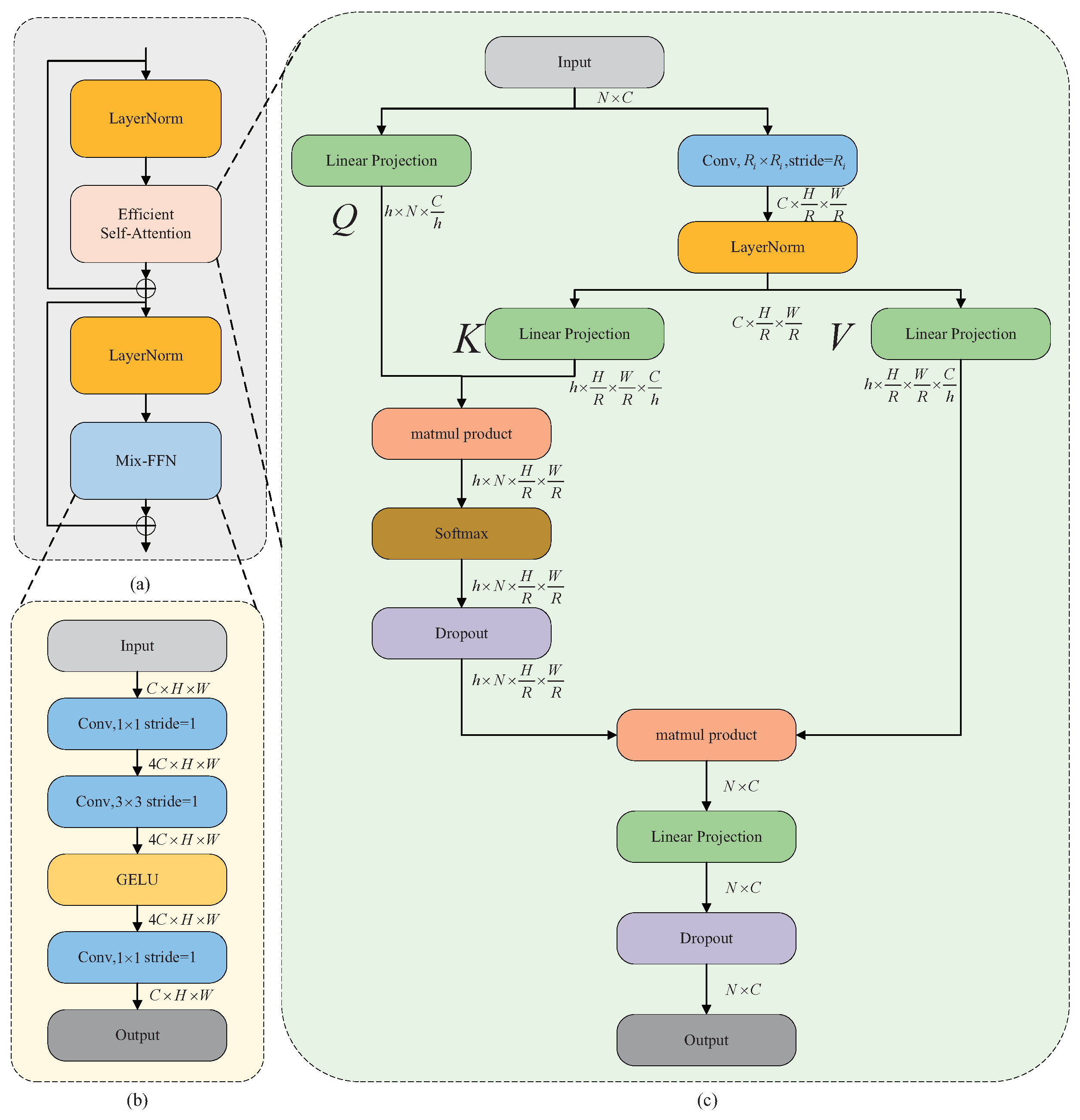
3.2. PVT-Based Encoder

Each stage of PVT contains two modules, namely Mix-Transformer and Overlap Patch Merging. Among them, the Overlap Patch Merging module is different from the traditional patch merging method and retains a certain spatial overlap area. With this setup, each newly generated feature block contains information from multiple adjacent original feature blocks around it. Therefore, this can better maintain the continuity and contextual information of local features. The size of the overlapping area can be modulated by adjusting the size and stride of the convolution kernel. In this paper, the dimension of the first branch convolution kernel is set to $(8,2,2,2)$. The dimension of the second branch convolution kernel is set to $(7,3,3,3)$. The dimension of the third branch convolution kernel is set to $(15,3,3,3)$. Stride is uniformly set to $(4,2,2,2)$. The structure of the Mix-Transformer is shown in Figure 2. Figure 2a shows the overall architecture. Assuming that the input feature map of layer l is $Z^{l-1}$, it first passes through the LayerNorm (LN) layer [79]. After the LN layer, the feature map undergoes processing by the Efficient Self-Attention (ESA) layer and is residually connected with $Z^{l-1}$ to obtain ${\widehat{Z}}^l$. After passing through the LN layer, the output feature map enters the Mixed Feed-Forward Network (Mix-FFN) layer. A residual connection with ${\widehat{Z}}^l$ then produces the ultimate feature map $Z^l$. The procedural formula is delineated as follows:

$$\begin{array}{c}{\widehat{Z}}^l=ESA\left(LN\left(Z^{l-1}\right)\right)+Z^{l-1}\hfill \\ Z^l=MixFFN\left(LN\left({\widehat{Z}}^l\right)\right)+{\widehat{Z}}^l\hfill \end{array}$$

(1)

The configuration of the ESA layer is shown in Figure 2c. The size of the input feature map is $N\times C$, with N denoting the total pixel count, calculated as $N=H\times W$ (where H and W are the feature map’s height and width, respectively), and C is the channel count. The input feature map goes through two branches. In one branch, the feature map is transformed into the query (Q) through linear projection with size $h\times N\times {\displaystyle \frac{C}{h}}$. In another branch, the feature map is passed through a convolution operation, usually using a larger kernel to diminish the resolution of the feature map. After downsampling, keys (K) and values (V) are generated through linear projection, and the size is reduced to $h\times {\displaystyle \frac{H}{R}}\times {\displaystyle \frac{W}{R}}\times {\displaystyle \frac{C}{h}}$. Reduce the computational complexity by adjusting R. In this paper, R is set to $(8,4,2,1)$ at different stages. The attention weights are then determined via matrix multiplication followed by a softmax operation, as detailed below.

$$Attention(Q,K,V)=Softmax\left({\displaystyle \frac{Q{K}^T}{\sqrt{d_k}}}\right)V$$

(2)

where $d_k$ signifies the key vector’s dimension. The attention mechanism’s output is subsequently transformed to the feature’s initial dimension via a linear projection layer. The ESA reduces computational demands while retaining the advantages of the self-attention mechanism in handling global dependencies.

The structure diagram of Mix-FFN is shown in Figure 2b. The input image size is $C\times H\times W$, which first passes through a $1\times 1$ convolution layer with a stride size of 1. This operation is mainly used to modify the number of channels of the feature map, from C channels to $4C$ channels, to add more feature information to subsequent layers. Following this, the feature map is processed by a $3\times 3$ convolutional layer with the same stride of 1. While this convolutional step preserves the spatial size of the feature map, it further delineates spatial characteristics. Subsequently, Gaussian Error Linear Unit (GELU) [80] is used as the activation function to introduce nonlinearity into the network and enhance the learning capabilities of the model. Finally, a $1\times 1$ convolution layer is passed with a stride of 1 to adjust the number of feature channels from $4C$ back to C, keeping the overall size of the feature map unchanged. Mix-FFN not only increases the nonlinear expression ability of features but also maintains sensitivity to spatial structure. The calculation formula is as follows:

$$\begin{array}{c}{F}^{\prime }=Con{v}_{1\times 1}\left(F\right)\hfill \\ F^{\prime \prime }=GELU\left(Con{v}_{3\times 3}\left(F^{\prime }\right)\right)\hfill \\ Output=Con{v}_{1\times 1}\left(F^{\prime \prime }\right)\hfill \end{array}$$

(3)

where $Con{v}_{1\times 1}$ and $Con{v}_{3\times 3}$ denote $1\times 1$ and $3\times 3$ convolution operations respectively. F represents the input feature map. $F^{\prime }$ and $F^{\prime \prime }$ represent the intermediate feature map.

3.3. Feature Fusion Module

The configuration of FFM is shown in Figure 3. The module first receives multi-scale input feature maps, with sizes $64\times 2^{i-1}\times {\displaystyle \frac{H}{2^i}}\times {\displaystyle \frac{W}{2^i}}$, $64\times 2^{i-1}\times {\displaystyle \frac{H}{2^{i+1}}}\times {\displaystyle \frac{W}{2^{i+1}}}$, and $64\times 2^{i-1}\times {\displaystyle \frac{H}{2^{i+2}}}\times {\displaystyle \frac{W}{2^{i+2}}}$ respectively, where i denotes the stage count, with $i=1,2,3,4$. Assume $F_s$, $F_m$ and $F_l$ represent small, medium and large size input feature maps respectively. $F_l$ first goes through one of the branches, including average pooling with stride 2 and $1\times 1$ convolution operation to downsample. Then pass another branch, including $1\times 1$ convolution to adjust the number of channels, and then further extract features through $3\times 3$ convolution with a stride of 2, and finally pass $1\times 1$ convolution. Concatenate the features of the two branches, followed by a channel count adjustment of the feature map to match $F_m$ using $1\times 1$ convolution, preparing it for further integration.

$F_m$ also passes through two branches. In the first branch, the channel is compressed through $1\times 1$ convolution, and then the spatial attention map is generated through Sigmoid and multiplied with $F_m$ to obtain the first branch output. In the second branch, the channel attention map is generated through the fully connected layer, ReLU, fully connected and Sigmoid, and multiplied with $F_m$ to get the output of the second branch. Finally, the outputs of the two branches are concatenated, followed by a channel adjustment using $1\times 1$ convolution, culminating in the feature map $F_m^{\prime }$.

The feature map $F_l$ first undergoes three pooling operations: average pooling, soft pooling [81] and max pooling to capture different types of spatial information. The results of these three pooling operations are fused and then processed through ReLU and Sigmoid activation functions to generate a set of attention weights. This set of attention weights is element-wise multiplied with $F_m^{\prime }$ and $F_l$ respectively. Once processed, the feature maps across three scales are combined, and a $1\times 1$ convolution adjusts the channel count to yield the final output, sized $64\times 2^{i-1}\times {\displaystyle \frac{H}{2^{i+1}}}\times {\displaystyle \frac{W}{2^{i+1}}}$, with i indicating the stage number, $i=1,2,3,4$. Multi-scale feature maps capture a spectrum of information, from intricate details to overarching global characteristics. The fusion operation makes this information complementary and enhances the expressive power of features.

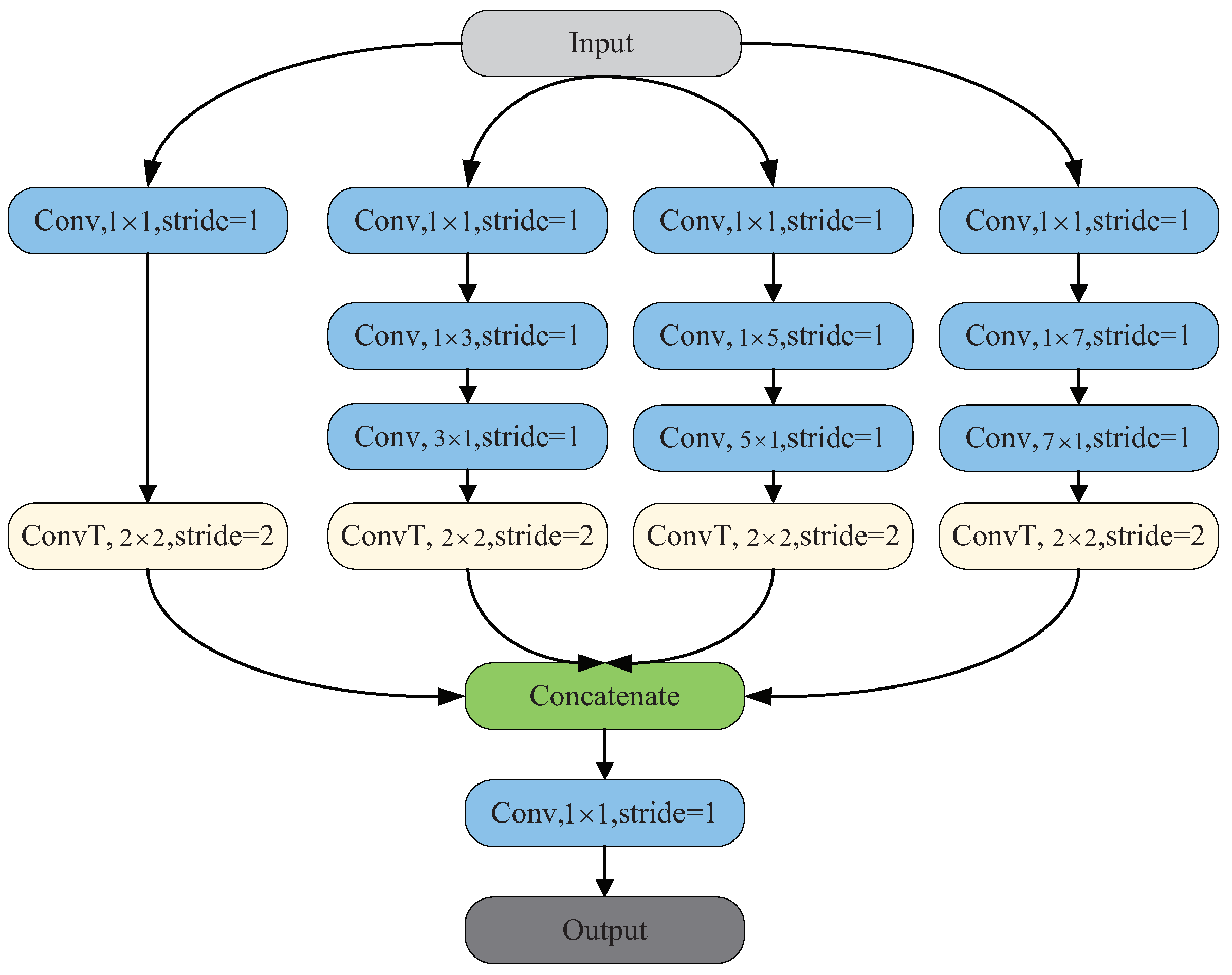
3.4. Multi-Scale Upsampling Module

Influenced by Inception v4 [27], the MSUM adopts a similar idea to process the input feature maps by parallelizing convolution and upsampling operations at different scales, and finally fuse them. This approach is utilized for capturing multi-scale spatial features. The network structure diagram is illustrated in Figure 4. Initially, the input feature map is processed through several $1\times 1$ convolutional layers in parallel, each with a stride of 1. These convolution operations do not modify the spatial dimensions of the feature map but can adjust the number of channels to prepare for subsequent multi-scale convolution. Then after convolution of $1\times n$ and $n\times 1$, $n=3,5,7$. Its receptive field is equivalent to a $3\times 3$, $5\times 5$, $7\times 7$ convolution kernel. However, this strategy of decomposing convolutions allows the module to achieve the same receptive field with less computational cost and capture finer-grained features in both vertical and horizontal directions. These feature maps are then upsampled via a $2\times 2$ deconvolution with a stride of 2, effectively enlarging both their width and height. Finally, the outputs of all branches are combined through a concatenation operation, followed by a passed through a $1\times 1$ convolutional layer to adjust the number of channels. Through such a process, the captured information at different scales can be integrated to obtain a richer feature representation. This improves the model’s capacity to capture details of RS images, thereby helping to improve the effect of semantic segmentation of RS images.

4. Experiment

4.1. Datasets

4.1.1. Potsdam Dataset

The Potsdam Dataset [82] encompasses 38 uniformly sized blocks, each block consists of a real image. The images of each block are of very high resolution, providing detailed urban surface information. The size of each image is $6000\times 6000$ pixels and the sampling distance is 5 cm. The image contains six categories, namely: buildings, cars, impervious surfaces, low vegetation, trees and clutter/background. For our study, 24 blocks are designated for the training set, while the remaining 14 serve as the test set. To facilitate training, all images are resized to dimensions of $512\times 512$ pixels.

4.1.2. Vaihingen Dataset

The Vaihingen Dataset [82] is provided by ISPRS and includes 33 blocks of different sizes, each block contains a true radiographic image (TOP) and a digital surface model (DSM). TOP contains three bands, corresponding to the near-infrared, red and green bands captured by the camera. The ground sampling distance of the dataset is 9 cm. The dataset categorizes the imagery into six classes: buildings, cars, impervious surfaces, low vegetation, trees, and clutter/background. The average dimension of the image is $2494\times 2064$ pixels. For our analysis, 16 images are allocated to the training set, and 17 are designated for the test set. To accommodate training processes, all images are resized to $512\times 512$ pixels.

4.1.3. LoveDA Dataset

The dataset contains a total of 5987 images, each with a resolution of $1024\times 1024$ pixels and a ground sampling distance of 0.3 m. It covers seven types of objects: buildings, agricultural, forest, background, roads, water, and barren. The dataset is divided into two parts: urban and rural. Among them, 2522 images are used as training sets, 1669 images are used as validation sets and 1796 images are used as test sets. Since the labeled data of the test set is not public, we choose to use the validation set for testing. The image size used for training and testing is $1024\times 1024$ pixels.

4.1.4. UAVid Dataset

The UAVid dataset is a collection specifically designed for urban scene semantic segmentation from UAV perspectives. It contains 420 high-resolution images, with two resolutions: $4096\times 2160$ and $3840\times 2160$ pixels. In this dataset, 200 images are used for training, 70 for validation, and 150 for testing. For ease of training, the images are cropped into small patches of $512\times 512$ pixels, which helps to process and train detailed urban landscapes more efficiently.

4.2. Evaluation Metrics

In the assessment of semantic segmentation models for RS images, frequently applied metrics are the F1 Score and the Mean Intersection over Union (MIoU). Their expressions are as follows:

$$\begin{array}{c}{F}_1=2\times {\displaystyle \frac{\mathrm{precision}\times \mathrm{recall}}{\mathrm{precision}+\mathrm{recall}}}\hfill \\ \\ \mathrm{IoU}={\displaystyle \frac{\mathrm{TP}}{\mathrm{TP}+\mathrm{FP}+\mathrm{FN}}}\hfill \end{array}$$

(4)

where TP denotes the positive class that is correctly predicted, FP denotes the negative class that is incorrectly predicted to be the positive class, FN denotes the positive class that is incorrectly predicted to be the negative class, and FN denotes the positive class that is incorrectly predicted to be the negative class. Precision represents the ratio of the predicted positive class that is the positive class, and Recall represents the ratio of the actual positive class that is correctly predicted to be the positive class. Their expressions are as follows:

$$\begin{array}{c}\mathrm{precision}={\displaystyle \frac{\mathrm{TP}}{\mathrm{TP}+\mathrm{FP}}}\hfill \\ \\ \mathrm{recall}={\displaystyle \frac{\mathrm{TP}}{\mathrm{TP}+\mathrm{FN}}}\hfill \end{array}$$

(5)

4.3. Implementation Details

Our experiments were completed in the environment of a single NVIDIA RTX 4080 graphics card, using PyTorch [83] as the primary framework for deep learning. For network parameter optimization, the Stochastic Gradient Descent (SGD) optimizer was selected, undertaking 40,000 iterations. We initialized the learning rate at 0.01, set the momentum to 0.9, and applied a weight decay of 0.0005 to foster optimal training outcomes. Furthermore, we also apply a polynomial decay learning rate scheduling strategy (PolyLR), reducing the learning rate progressively from its initial setting to 1 × 10⁻⁴. To maintain uniformity in input data, all images were resized to $512\times 512$ pixels, and the batch size was established at 4, striking a balance between training efficiency and memory consumption.

4.4. Ablation Study

To assess the effectiveness of the proposed encoder and its two key components, ablation studies were carried out on the Vaihingen dataset and the LoveDA dataset. Taking the network of single-branch PVT as the encoder combined with UNet as the benchmark, it is referred to as P_UNet for short. The multi-branch PVT encoder module is referred to as MBT. Among them, the number of execution times of Mix-Transformer in each branch of the encoder part is $(3,4,6,3)$.

4.4.1. Effect of Multi-Branch PVT

As shown in

Table 1. Ablation Experiments of the Proposed Modules on the Vaihingen Dataset.

Model Name	Modules			IoU (%)					Evaluation Index
	MBT	FFM	MSUM	Impervious Surface	Building	Low Vegetation	Tree	Car	MIoU (%)	mF1 (%)
P_UNet				80.9	84.98	69.28	78.29	55.02	73.69	84.56
	✓			81.75	85.6	69.32	78.44	61.17	75.26	85.58
	✓	✓		82.69	87.42	69.38	78.76	63.75	76.4	86.23
	✓	✓	✓	84.25	88.14	69.62	79	64.34	77.07	86.76

. After the introduction of MBT, the segmentation result improved from 73.69% to 75.26% in the MIoU index, an increase of 1.57%. The mF1 indicator increased from 84.56% to 85.58%, an increase of 1.02%. Among them, the IoU of “Car” increased significantly from 55.02% before the module was introduced to 61.17% after the module was introduced, an increase of 6.15%. Followed by “Impervious Surface”, the IoU increased by 0.85%. The visualized segmentation results are shown in Figure 5. In the first row, when cars are relatively dense, each “Car” can still be segmented accurately. In the second row, “Car” can also be segmented when there is shadow occlusion by “Tree”. In the third row, when the “Car” is dense and there are shadows, good segmentation results can also be achieved. Experiments show that the introduction of MBT enhances the precision of segmenting variously scaled targets, especially targets with smaller sizes.

As shown in

Table 2. Ablation Experiments of the Proposed Modules on the LoveDA Dataset.

Method Name	Modules			Evaluation Index
	MBT	FFM	MSUM	MIoU (%)	mF1 (%)
P_UNet				43.47	59.7
	✓			44.32	60.78
	✓	✓		45.12	61.5
	✓	✓	✓	45.97	62.33

. After introducing MBT on the LoveDA dataset, the segmentation results increased from 43.47% to 44.32% on MIoU, an increase of 0.85%. The mF1 index increased from 59.7% to 60.78%, an increase of 1.08%. The segmentation results are shown in Figure 6 In the first row, the building outline is accurately segmented. In the second row, objects of different categories are accurately segmented. In the third row, objects of different scales are accurately segmented. This also proves the effectiveness of MBT.

4.4.2. Effect of FFM

The experimental results are shown in Table 1. By introducing FFM based on MBT, the segmentation result increased from 75.26% to 76.4% in the MIoU index, an increase of 1.14%. The mF1 indicator increased from 85.58% to 86.23%, an increase of 0.65%. Among them, the IoU value of “Car” increased the most, increasing by 2.58%. Followed by “Building”, an increase of 1.82%. The experimental results are illustrated in Figure 5. In the first row, the model effectively distinguishes between “Building” and “Low Vegetation” categories and accurately segments them. In the second row, the model similarly differentiates between “Tree” and “Impervious Surface” without any false detections. In the third row, the model accurately segments “Tree” and “Low Vegetation” even in the presence of shadows. The outcomes illustrate that the FFM adeptly merges features across various strata, augmenting the model’s proficiency in identifying nuances and edges.

As shown in Table 2, after introducing FFM on the LoveDA dataset, the segmentation results increased from 44.32% to 45.12% on MIoU, an increase of 0.8%. The mF1 index increased from 60.78% to 61.5%, an increase of 0.72%. The visualization results are shown in Figure 6. In the first row, the segmentation is completed when “Building” and “Background” are very close. In the second row, the boundary between “Forest” and “Agricultural” is also accurately segmented. In the third row, a better segmentation effect is achieved for the complex situation of different objects. Similarly, the effectiveness of the FFM module is proved.

4.4.3. Effect of MSUM

As shown in Table 1. Finally, the MSUM module was introduced, and the segmentation result increased from 76.4% to 77.07% in the MIoU index, an increase of 0.67%. The mF1 indicator increased from 86.23% to 86.76%, an increase of 0.53%. The IoU value of each category has improved. Among them, the “Impervious Surface” category has the most obvious increase, increasing by 1.56%, followed by the “Building” category, increasing by 0.72%. The visualization results are shown in Figure 5. In the first row, the model accurately segments the boundaries between “Building” and “Low Vegetation” even in ambiguous regions. In the second row, it precisely detects the fine details of the “Forest”. In the third row, the model successfully avoids false detections in the case of highly similar appearances between “Clutter” and “Building”. The results show that by combining upsampling features at different scales, the model’s ability to capture targets of different sizes is improved, and the overall segmentation accuracy is improved.

As shown in Table 2, after introducing MSUM on the LoveDA dataset, the segmentation results increased from 45.12% to 45.97% in MIoU, an increase of 0.85%. The mF1 index increased from 61.5% to 62.33%, an increase of 0.83%. The visualization results are shown in Figure 6. In the first row, the model accurately extracts “Agricultural” and “Background” regions even when their boundaries are ambiguous. In the second and third rows, it precisely extracts the detailed features of “Building” contours. Similarly, the effectiveness of the MSUM module is proved.

4.5. Comparison with State-of-the-Art Methods

In this section, we compare our network with state-of-the-art methods, including: UNet [30], FCN [29], DANet [33], DeepLabv3+ [84], PSPNet [31], SegFormer [38], BiSeNet V2 [85], ST-UNet [65], SSNet [69], STDSNet [66], and DSHNet [74]. Among them, UNet, FCN, DANet, DeepLabv3+, PSPNet, and BiSeNet V2 are CNN-based models, Segformer is a Transformer-based model, and ST-UNet, SSNet, STDSNet, and DSHNet are hybrid models based on CNN and Transformer. To ensure the validity of the experiment, the backbone based on the CNN model uniformly uses ResNet-50. SegFormer uses MIT-B5 as its backbone. ST-UNet uses ResNet-50 and Swin-B as the backbone. SSNet employs MIT-B5 and SegNext as its backbones, while STDSNet utilizes Swin-B and DSHNet adopts ViT-Base. All models are not pre-trained.

4.5.1. Results on the Vaihingen Dataset

The numerical comparison results between our model and other methods on the Vaihingen dataset are shown in

Table 3. Comparison of Seg mentation Results on the Vaihingen Dataset.

Method	Backbone	IoU (%)					Evaluation Index
		Impervious Surface	Building	Low Vegetation	Tree	Car	MIoU (%)	mF1 (%)
UNet	-	79.58	84.54	66.68	77.91	49.92	71.73	82.89
FCN	ResNet-50	78.71	81.75	65.98	77.41	54.05	71.58	83
DANet	ResNet-50	81.31	85.36	68.2	78.5	53.06	73.29	84.03
DeepLabv3+	ResNet-50	82.09	86.88	65.69	75.83	55.82	73.26	84.07
PSPNet	ResNet-50	81.55	83.92	66.3	74.83	54.4	72.2	83.38
SegFormer	MIT-B5	83.09	88.01	69.45	78.49	53.4	74.49	85.04
BiSeNet V2	-	81.68	86.81	69.5	78.04	56.55	74.52	84.95
ST-UNet	ResNet-50+Swin-B	83.38	88.12	67.69	78.08	57.81	75.02	85.26
SSNet	MIT-B5+SegNext	84.19	87.18	70.17	78.94	58.72	75.84	85.76
STDSNet	Swin-B	84.19	87.3	70.4	78.16	60.39	76.09	85.94
DSHNet	ViT-Base	82.48	87.64	69.33	78.94	57.8	75.24	85.44
MBT-UNet	MBT	84.25	88.14	69.62	79	64.34	77.07	86.76

. The results show that our method achieves the best performance in both MIoU and mF1 metrics. Except for the “Low Vegetation” category, our method outperforms others in IoU metrics for all other categories. It is evident from Table 3 that the detection effects of UNet and FCN models based on traditional convolution are poor. DANet and DeepLabv3+ models have improved some detection effects by introducing attention mechanisms or feature pyramid modules. The performance of the Transformer-based SegFormer model surpasses that of conventional convolution-based models. ST-UNet, SSNet, STDSNet, and DSHNet combine Transformer and CNN, generally outperforming single-model methods. Compared to the next best method, STDSNet, our method improved the MIoU metric from 76.09% to 77.07%, an increase of 0.98%. The mF1 metric improved from 85.94% to 86.76%, an increase of 0.82%. The “Car” category saw the most significant improvement, with an increase of 3.95%. Comparative experimental outcomes are depicted in Figure 7. In the first, second, and fourth columns, the model can accurately segment dense cars. In the third and sixth columns, even when “Low Vegetation” and “Tree” interfere with each other, they can still be segmented well. In the fifth column, “Car” is accurately segmented under the interference of “Low Vegetation”. The experimental findings indicate that our approach enhances the precision of identifying targets across multiple scales, with a notable improvement in detecting smaller objects. At the same time, the detection ability of details and boundaries is improved.

4.5.2. Results on the Potsdam Dataset

The numerical comparison results between our model and other methods on the Potsdam dataset are shown in

Table 4. Comparison of Segmentation Re sults on the Potsdam Dataset.

Method	Backbone	IoU (%)					Evaluation Index
		Impervious Surface	Building	Low Vegetation	Tree	Car	MIoU (%)	mF1 (%)
UNet	-	79.61	82.85	69.66	69.86	84.06	77.21	87.23
FCN	ResNet-50	79.73	84.94	69.44	67.5	83.14	76.95	86.79
DANet	ResNet-50	81.4	87.4	70.84	68.99	83.14	78.35	87.8
DeepLabv3+	ResNet-50	79.63	87.02	69.98	69.96	85.07	78.33	88.06
PSPNet	ResNet-50	80.6	84.39	68.87	69.28	84.06	77.44	87.11
SegFormer	MIT-B5	80.07	84.64	71.03	68.24	83.74	77.54	87.18
BiSeNet V2	-	79.35	84.47	67.03	65.84	82.68	75.87	86.04
ST-UNet	ResNet-50+Swin-B	81.47	86.82	70.12	69.78	84.9	78.62	87.84
SSNet	MIT-B5+SegNext	81.32	85.26	71.94	70.07	84.18	78.55	87.88
STDSNet	Swin-B	81.25	87.84	71.99	70.06	82.84	78.80	87.97
DSHNet	ViT-Base	81.31	86.56	70.15	71.46	84.94	78.88	88.05
MBT-UNet	MBT	81.88	88.24	72.19	70.38	85.14	79.57	88.44

. It further demonstrates the effectiveness of our approach. The results show that our method achieves the best performance in both the MIoU and mF1 metrics. Except for the “Tree” category, our method outperforms others in IoU metrics for all other categories. Compared to the next best method, DSHNet, our method improved the MIoU metric from 78.88% to 79.57%, an increase of 0.68%. The mF1 metric improved from 88.05% to 88.44%, an increase of 0.39%. The “Low Vegetation” category saw the most significant improvement, with an increase of 2.04%. The comparison of visualization results is shown in Figure 8. In the first and second columns, “Car” is interfered with by “Tree” or “Low Vegetation”, and the model can detect and segment it well. In the third and fourth columns, despite “Low Vegetation” having indistinct edges with the background and “Tree”, it is still segmented precisely. In the sixth column, our method can extract the details of “Low Vegetation” and “Tree” to improve segmentation accuracy. The experiment also proved the effectiveness of MBT-UNet.

4.5.3. Results on the LoveDA Dataset

Table 5. Comparison of Segmentation Results on the LoveDA Dataset.

Method	Backbone	IoU (%)							Evaluation Index
		Background	Building	Road	Water	Barren	Forest	Agricultural	MIoU (%)	mF1 (%)
UNet	-	48.45	48.72	43.07	42.65	21.77	37.85	42.84	40.76	57.35
FCN	ResNet-50	46.74	46.25	45.45	40.05	24.98	40.44	39.12	40.43	57.2
DaNet	ResNet-50	48.97	53.36	48.66	45.43	16.04	38.67	40.57	41.67	57.7
Deeplabv3+	ResNet-50	50.34	47.29	49.07	52.06	22.67	37.14	47.47	43.72	60.14
PSPNet	ResNet-50	45.53	42.04	52.82	56.08	12.36	37.94	43.53	41.47	57.2
Segformer	MIT-B5	51.02	53.74	53.78	46.82	17.53	37.75	47.37	44.00	60.02
BiseNetv2	-	46.31	50.18	37.14	53.06	21.14	35.10	44.89	41.12	57.49
ST-UNet	ResNet50+Swin-B	51.20	53.50	48.24	57.09	23.61	39.13	41.09	44.84	61.06
SSNet	MIT-B5+SegNext	50.08	54.22	49.37	56.88	25.18	33.22	45.34	44.90	61.17
STDSNet	Swin-B	51.86	54.12	46.01	55.03	24.8	40.58	43.06	45.07	61.35
DSHNet	ViT-Base	48.25	47.43	53.95	56.76	25.4	40.7	44.45	45.28	61.69
MBT-UNet	MBT	51.92	54.33	47.15	57.68	26.16	41.06	43.50	45.97	62.33

gives the numerical comparison of our method with other state-of-the-art methods on the LoveDA Dataset. Our method achieves the best performance in both MIoU and mF1 indicators. In terms of individual categories, it achieves the best performance in all categories except “Road” and “Agricultural”. Compared to the next best method, DSHNet, our method improved the MIoU metric from 45.28% to 45.97%, an increase of 0.69%. The mF1 metric improved from 61.69% to 62.33%, an increase of 0.64%. The visualization results are shown in Figure 9. In the first, fourth and sixth columns, other methods have missed detection when segmenting complex objects, while our method can accurately segment them. In the second, third and fifth columns, when faced with similar situations of “Barren” and “Agricultural”, other methods have different degrees of misdetection, but our method can accurately segment the corresponding boundaries. The experiment also proves the effectiveness of the proposed method.

4.5.4. Results on the UAVid Dataset

Table 6. Comparison of Segmentation Results on the UAVid Dataset.

Method	Backbone	IoU (%)								Evaluation Index
		Clutter	Building	Road	Tree	Low Vegetation	Moving Car	Static Car	Human	MIoU (%)	mF1 (%)
UNet	-	92.28	82.92	76.17	65.8	59.66	54.16	39.04	13.45	60.44	79.09
FCN	ResNet-50	90.93	82.58	72.08	61.99	58.26	49.34	37.7	14.48	58.42	74.67
DaNet	ResNet-50	91.88	82.41	75.64	65.74	61.77	52.08	40.96	12.87	60.42	77.66
Deeplabv3+	ResNet-50	92.78	85.28	76.98	68.33	58.99	56.52	36.69	15.89	61.43	79.58
PSPNet	ResNet-50	91.78	81.91	75.97	65.26	64.12	50.81	31.61	10.12	58.95	76.22
Segformer	MIT-B5	92.2	83.67	76.79	69.36	62.03	58.44	42.77	18.76	63.00	80.87
BiseNetv2	-	93.15	85.07	77.34	69.36	60.99	56.01	38.19	16.63	62.09	79.59
ST-UNet	ResNet50+Swin-B	93.23	85.02	77.61	69.76	62.86	57.04	37.79	19.61	62.87	80.18
SSNet	MIT-B5+SegNext	91.93	85.19	77.67	69.61	63.11	58.26	40.96	20.87	63.45	81.08
STDSNet	Swin-B	92.54	84.75	76.13	70.12	63.5	59.1	43.15	19.87	63.65	81.26
DSHNet	ViT-Base	91.29	84.22	76.6	69.42	63.68	59.25	41.17	18.84	63.06	80.96
MBT-UNet	MBT	93.46	85.71	77.28	70.47	63.07	60.82	43.35	21.43	64.45	81.79

shows the numerical comparison of our method with other state-of-the-art methods on the UAVid Dataset. Our method achieves the best performance in both MIoU and mF1. In terms of individual categories, except for the “Road” and “Low Vegetation” categories, it achieves the best performance in other categories. Compared to the next best method, STDSNet, our method improved the MIoU metric from 63.65% to 64.45%, an increase of 0.8%. The mF1 metric improved from 81.26% to 81.79%, an increase of 0.53%. The visualization results are shown in Figure 10. In the first, third, and fourth columns, there is mutual occlusion between the “Tree” and “Vegetation” categories. Compared with other methods, our method can accurately segment the two. In the second column, the “Moving Car” and “Static Car” look very similar. Other methods have different degrees of false detection. Our method accurately segments the two based on context information. The above four sets of experiments fully demonstrate the effectiveness of MBT-UNet.

4.5.5. Efficiency Analysis

To comprehensively evaluate the performance of the proposed method.

Table 7. Comparison of Model Parameters, FLOPs and FPS.

Method	Parameters (M)	FLOPs (G)	FPS
UNet	28.99	203	72
FCN	47.13	198	75
DANet	47.46	211	69
DeepLabv3+	41.22	177	70
PSPNet	46.6	179	73
SegFormer	81.98	75	98
BiSeNet V2	3.35	12	232
ST-UNet	183.27	236	48
SSNet	61.47	184	64
STDSNet	138.69	331	36
DSHNet	129.34	287	42
MBT-UNet	108.22	187	66

shows the performance indicators of the method under the same hardware conditions. Assessment is conducted via model parameters, frame per second(FPS) and floating point operations (FLOPs). Table 7 reveals that Transformer-based models possess a greater number of parameters compared to those based on CNN. BiSeNet V2 has the lowest model parameters and FLOPs indicators. The number of model parameters and FLOPs of STDSNet are relatively high. Our model has 21.95% fewer parameters and 43.47% fewer FLOPs than STDSNet. At the same time, our model’s inference speed reaches 66 FPS, which can basically meet the requirements of real-time inference. While the substantial parameter count could restrict our model’s deployment on embedded and mobile platforms, its significant contribution to the domain of RS image semantic segmentation remains undiminished.

5. Conclusions

In this article, we propose a novel deep learning model that combines a multi-branch PVT encoder and UNet, designed to enhance the accuracy of semantic segmentation in RS imagery. The introduction of a multi-branch PVT encoder strengthens the capture of multi-scale features, especially for small-scale targets. Through the design of the FFM, multi-scale features are guided and fused, so that the model can show higher segmentation accuracy in processing details and edges. At the same time, the introduced MSUM further bolsters the model’s capability to identify features of different sizes. Experiments on the ISPRS Vaihingen dataset, Potsdam dataset, LoveDA dataset and UAVid dataset show that our model exhibits excellent performance in all indicators compared with other methods. However, our model still has problems such as a large number of parameters. In future work, we will continue to streamline the network structure to achieve a higher balance of efficiency and accuracy to adapt to larger and more RS image processing scenarios.

References

1. Amani, M.; Mahdavi, S.; Kakooei, M.; Ghorbanian, A.; Brisco, B.; DeLancey, E.R.; Toure, S.; Reyes, E.L. Wetland Change Analysis in Alberta, Canada Using Four Decades of Landsat Imagery. IEEE J. Sel. Top. Appl. Earth Obs. Remote Sens. 2021, 14, 10314–10335. [Google Scholar] [CrossRef]
2. Xu, C.; Wang, J.; Sang, Y.; Li, K.; Liu, J.; Yang, G. An Effective Deep Learning Model for Monitoring Mangroves: A Case Study of the Indus Delta. Remote Sens. 2023, 15, 2220. [Google Scholar] [CrossRef]
3. Jung, H.; Choi, H.S.; Kang, M. Boundary Enhancement Semantic Segmentation for Building Extraction From Remote Sensed Image. IEEE Trans. Geosci. Remote Sens. 2022, 60, 1–12. [Google Scholar] [CrossRef]
4. Wang, L.; Fang, S.; Meng, X.; Li, R. Building Extraction With Vision Transformer. IEEE Trans. Geosci. Remote Sens. 2022, 60, 1–11. [Google Scholar] [CrossRef]
5. Huan, H.; Liu, Y.; Xie, Y.; Wang, C.; Xu, D.; Zhang, Y. MAENet: Multiple Attention Encoder–Decoder Network for Farmland Segmentation of Remote Sensing Images. IEEE Geosci. Remote Sens. Lett. 2022, 19, 1–5. [Google Scholar] [CrossRef]
6. Zhang, R.; Chen, J.; Feng, L.; Li, S.; Yang, W.; Guo, D. A Refined Pyramid Scene Parsing Network for Polarimetric SAR Image Semantic Segmentation in Agricultural Areas. IEEE Geosci. Remote Sens. Lett. 2022, 19, 1–5. [Google Scholar] [CrossRef]
7. Yu, Z.; Wang, J.; Yang, X.; Ma, J. Superpixel-Based Style Transfer Method for Single-Temporal Remote Sensing Image Identification in Forest Type Groups. Remote Sens. 2023, 15, 3875. [Google Scholar] [CrossRef]
8. Liu, T.; Yao, L.; Qin, J.; Lu, J.; Lu, N.; Zhou, C. A Deep Neural Network for the Estimation of Tree Density Based on High-Spatial Resolution Image. IEEE Trans. Geosci. Remote Sens. 2022, 60, 1–11. [Google Scholar] [CrossRef]
9. Han, W.; Li, J.; Wang, S.; Zhang, X.; Dong, Y.; Fan, R.; Zhang, X.; Wang, L. Geological Remote Sensing Interpretation Using Deep Learning Feature and an Adaptive Multisource Data Fusion Network. IEEE Trans. Geosci. Remote Sens. 2022, 60, 1–14. [Google Scholar] [CrossRef]
10. Chen, X.; Yao, X.; Zhou, Z.; Liu, Y.; Yao, C.; Ren, K. DRs-UNet: A Deep Semantic Segmentation Network for the Recognition of Active Landslides from InSAR Imagery in the Three Rivers Region of the Qinghai–Tibet Plateau. Remote Sens. 2022, 14, 1848. [Google Scholar] [CrossRef]
11. Zhong, H.F.; Sun, Q.; Sun, H.M.; Jia, R.S. NT-Net: A Semantic Segmentation Network for Extracting Lake Water Bodies From Optical Remote Sensing Images Based on Transformer. IEEE Trans. Geosci. Remote Sens. 2022, 60, 1–13. [Google Scholar] [CrossRef]
12. Liu, S.; Li, M.; Xu, M.; Zeng, Z. An Improved Lightweight U-Net for Sea Ice Lead Extraction From Multipolarization SAR Images. IEEE Geosci. Remote Sens. Lett. 2023, 20, 1–5. [Google Scholar] [CrossRef]
13. Cui, L.; Jing, X.; Wang, Y.; Huan, Y.; Xu, Y.; Zhang, Q. Improved Swin Transformer-Based Semantic Segmentation of Postearthquake Dense Buildings in Urban Areas Using Remote Sensing Images. IEEE J. Sel. Top. Appl. Earth Obs. Remote Sens. 2023, 16, 369–385. [Google Scholar] [CrossRef]
14. Liu, X.; Peng, Y.; Lu, Z.; Li, W.; Yu, J.; Ge, D.; Xiang, W. Feature-Fusion Segmentation Network for Landslide Detection Using High-Resolution Remote Sensing Images and Digital Elevation Model Data. IEEE Trans. Geosci. Remote Sens. 2023, 61, 1–14. [Google Scholar] [CrossRef]
15. Pal, S.K.; Ghosh, A.; Shankar, B.U. Segmentation of Remotely Sensed Images with Fuzzy Thresholding, and Quantitative Evaluation. Int. J. Remote Sens. 2000, 21, 2269–2300. [Google Scholar] [CrossRef]
16. Yu, Q.; Clausi, D.A. SAR Sea-Ice Image Analysis Based on Iterative Region Growing Using Semantics. IEEE Trans. Geosci. Remote Sens. 2007, 45, 3919–3931. [Google Scholar] [CrossRef]
17. Ferraioli, G. Multichannel InSAR Building Edge Detection. IEEE Trans. Geosci. Remote Sens. 2010, 48, 1224–1231. [Google Scholar] [CrossRef]
18. Wang, Y.; Yu, W.; Fang, Z. Multiple Kernel-Based SVM Classification of Hyperspectral Images by Combining Spectral, Spatial, and Semantic Information. Remote Sens. 2020, 12, 120. [Google Scholar] [CrossRef]
19. Zheng, C.; Wang, L. Semantic Segmentation of Remote Sensing Imagery Using Object-Based Markov Random Field Model With Regional Penalties. IEEE J. Sel. Top. Appl. Earth Obs. Remote Sens. 2015, 8, 1924–1935. [Google Scholar] [CrossRef]
20. Zheng, C.; Zhang, Y.; Wang, L. Semantic Segmentation of Remote Sensing Imagery Using an Object-Based Markov Random Field Model With Auxiliary Label Fields. IEEE Trans. Geosci. Remote Sens. 2017, 55, 3015–3028. [Google Scholar] [CrossRef]
21. Zhang, P.; Li, M.; Wu, Y.; Li, H. Hierarchical Conditional Random Fields Model for Semisupervised SAR Image Segmentation. IEEE Trans. Geosci. Remote Sens. 2015, 53, 4933–4951. [Google Scholar] [CrossRef]
22. Du, S.; Zhang, F.; Zhang, X. Semantic Classification of Urban Buildings Combining VHR Image and GIS Data: An Improved Random Forest Approach. ISPRS J. Photogramm. Remote Sens. 2015, 105, 107–119. [Google Scholar] [CrossRef]
23. Simonyan, K.; Zisserman, A. Very Deep Convolutional Networks for Large-Scale Image Recognition. arXiv 2014, arXiv:1409.1556. [Google Scholar]
24. Szegedy, C.; Liu, W.; Jia, Y.; Sermanet, P.; Reed, S.; Anguelov, D.; Erhan, D.; Vanhoucke, V.; Rabinovich, A. Going Deeper with Convolutions. arXiv 2014, arXiv:1409.4842. [Google Scholar]
25. Ioffe, S.; Szegedy, C. Batch Normalization: Accelerating Deep Network Training by Reducing Internal Covariate Shift. arXiv 2015, arXiv:1502.03167. [Google Scholar]
26. Szegedy, C.; Vanhoucke, V.; Ioffe, S.; Shlens, J.; Wojna, Z. Rethinking the Inception Architecture for Computer Vision. In Proceedings of the 2016 IEEE Conference on Computer Vision and Pattern Recognition (CVPR), Las Vegas, NV, USA, 27–30 June 2016; pp. 2818–2826. [Google Scholar] [CrossRef]
27. Szegedy, C.; Ioffe, S.; Vanhoucke, V.; Alemi, A. Inception-v4, Inception-ResNet and the Impact of Residual Connections on Learning. Proc. AAAI Conf. Artif. Intell. 2017, 31. [Google Scholar] [CrossRef]
28. He, K.; Zhang, X.; Ren, S.; Sun, J. Deep Residual Learning for Image Recognition. In Proceedings of the 2016 IEEE Conference on Computer Vision and Pattern Recognition (CVPR), Las Vegas, NV, USA, 27–30 June 2016; pp. 770–778. [Google Scholar] [CrossRef]
29. Long, J.; Shelhamer, E.; Darrell, T. Fully Convolutional Networks for Semantic Segmentation. In Proceedings of the 2015 IEEE Conference on Computer Vision and Pattern Recognition (CVPR), Boston, MA, USA, 7–12 June 2015; pp. 3431–3440. [Google Scholar] [CrossRef]
30. Ronneberger, O.; Fischer, P.; Brox, T. U-Net: Convolutional Networks for Biomedical Image Segmentation. In Proceedings of the Medical Image Computing and Computer-Assisted Intervention–MICCAI 2015, Munich, Germany, 5–9 October 2015; pp. 234–241. [Google Scholar] [CrossRef]
31. Zhao, H.; Shi, J.; Qi, X.; Wang, X.; Jia, J. Pyramid Scene Parsing Network. In Proceedings of the 2017 IEEE Conference on Computer Vision and Pattern Recognition (CVPR), Honolulu, HI, USA, 21–26 July 2017; pp. 6230–6239. [Google Scholar] [CrossRef]
32. Xiao, T.; Liu, Y.; Zhou, B.; Jiang, Y.; Sun, J. Unified Perceptual Parsing for Scene Understanding. In Proceedings of the European Conference on Computer Vision (ECCV), Munich, Germany, 8–14 September 2018; pp. 418–434. [Google Scholar]
33. Fu, J.; Liu, J.; Tian, H.; Li, Y.; Bao, Y.; Fang, Z.; Lu, H. Dual Attention Network for Scene Segmentation. In Proceedings of the 2019 IEEE/CVF Conference on Computer Vision and Pattern Recognition (CVPR), Long Beach, CA, USA, 15–20 June 2019; pp. 3141–3149. [Google Scholar] [CrossRef]
34. Vaswani, A.; Shazeer, N.; Parmar, N.; Uszkoreit, J.; Jones, L.; Gomez, A.N.; Kaiser, Ł.; Polosukhin, I. Attention Is All You Need. In Proceedings of the 31st International Conference on Neural Information Processing Systems, Long Beach, CA, USA, 4–9 December 2017; pp. 6000–6010. [Google Scholar]
35. Carion, N.; Massa, F.; Synnaeve, G.; Usunier, N.; Kirillov, A.; Zagoruyko, S. End-to-End Object Detection with Transformers. In Proceedings of the Computer Vision–ECCV 2020, Glasgow, UK, 23–28 August 2020; pp. 213–229. [Google Scholar] [CrossRef]
36. Liu, Z.; Lin, Y.; Cao, Y.; Hu, H.; Wei, Y.; Zhang, Z.; Lin, S.; Guo, B. Swin Transformer: Hierarchical Vision Transformer Using Shifted Windows. In Proceedings of the 2021 IEEE/CVF International Conference on Computer Vision (ICCV), Montreal, BC, Canada, 11–17 October 2021; pp. 9992–10002. [Google Scholar] [CrossRef]
37. Zhang, Q.; Yang, Y.B. ResT: An Efficient Transformer for Visual Recognition. Proc. Adv. Neural Inf. Process. Syst. 2021, 34, 15475–15485. [Google Scholar]
38. Xie, E.; Wang, W.; Yu, Z.; Anandkumar, A.; Alvarez, J.M.; Luo, P. SegFormer: Simple and Efficient Design for Semantic Segmentation with Transformers. Proc. Adv. Neural Inf. Process. Syst. 2021, 34, 12077–12090. [Google Scholar]
39. Wang, J.; Sun, K.; Cheng, T.; Jiang, B.; Deng, C.; Zhao, Y.; Liu, D.; Mu, Y.; Tan, M.; Wang, X.; et al. Deep High-Resolution Representation Learning for Visual Recognition. IEEE Trans. Pattern Anal. Mach. Intell. 2021, 43, 3349–3364. [Google Scholar] [CrossRef]
40. Yi, Y.; Zhang, Z.; Zhang, W.; Zhang, C.; Li, W.; Zhao, T. Semantic Segmentation of Urban Buildings from VHR Remote Sensing Imagery Using a Deep Convolutional Neural Network. Remote Sens. 2019, 11, 1774. [Google Scholar] [CrossRef]
41. Ding, L.; Tang, H.; Bruzzone, L. LANet: Local Attention Embedding to Improve the Semantic Segmentation of Remote Sensing Images. IEEE Trans. Geosci. Remote Sens. 2021, 59, 426–435. [Google Scholar] [CrossRef]
42. Xu, Z.; Zhang, W.; Zhang, T.; Li, J. HRCNet: High-Resolution Context Extraction Network for Semantic Segmentation of Remote Sensing Images. Remote Sens. 2021, 13, 71. [Google Scholar] [CrossRef]
43. Yang, X.; Li, S.; Chen, Z.; Chanussot, J.; Jia, X.; Zhang, B.; Li, B.; Chen, P. An Attention-Fused Network for Semantic Segmentation of Very-High-Resolution Remote Sensing Imagery. ISPRS J. Photogramm. Remote Sens. 2021, 177, 238–262. [Google Scholar] [CrossRef]
44. Li, R.; Zheng, S.; Zhang, C.; Duan, C.; Wang, L.; Atkinson, P.M. ABCNet: Attentive Bilateral Contextual Network for Efficient Semantic Segmentation of Fine-Resolution Remotely Sensed Imagery. ISPRS J. Photogramm. Remote Sens. 2021, 181, 84–98. [Google Scholar] [CrossRef]
45. Sun, L.; Cheng, S.; Zheng, Y.; Wu, Z.; Zhang, J. SPANet: Successive Pooling Attention Network for Semantic Segmentation of Remote Sensing Images. IEEE J. Sel. Top. Appl. Earth Obs. Remote Sens. 2022, 15, 4045–4057. [Google Scholar] [CrossRef]
46. Li, R.; Zheng, S.; Duan, C.; Su, J.; Zhang, C. Multistage Attention ResU-Net for Semantic Segmentation of Fine-Resolution Remote Sensing Images. IEEE Geosci. Remote Sens. Lett. 2022, 19, 1–5. [Google Scholar] [CrossRef]
47. Li, R.; Zheng, S.; Zhang, C.; Duan, C.; Su, J.; Wang, L.; Atkinson, P.M. Multiattention Network for Semantic Segmentation of Fine-Resolution Remote Sensing Images. IEEE Trans. Geosci. Remote Sens. 2022, 60, 1–13. [Google Scholar] [CrossRef]
48. Chen, Y.; Wang, Y.; Xiong, S.; Lu, X.; Zhu, X.X.; Mou, L. Integrating Detailed Features and Global Contexts for Semantic Segmentation in Ultrahigh-Resolution Remote Sensing Images. IEEE Trans. Geosci. Remote Sens. 2024, 62, 1–14. [Google Scholar] [CrossRef]
49. Hu, L.; Zhou, X.; Ruan, J.; Li, S. ASPP+-LANet: A Multi-Scale Context Extraction Network for Semantic Segmentation of High-Resolution Remote Sensing Images. Remote Sens. 2024, 16, 1036. [Google Scholar] [CrossRef]
50. Wang, Q.; Chen, W.; Huang, Z.; Tang, H.; Yang, L. MultiSenseSeg: A Cost-Effective Unified Multimodal Semantic Segmentation Model for Remote Sensing. IEEE Trans. Geosci. Remote Sens. 2024, 62, 1–24. [Google Scholar] [CrossRef]
51. Xie, J.; Pan, B.; Xu, X.; Shi, Z. MiSSNet: Memory-Inspired Semantic Segmentation Augmentation Network for Class-Incremental Learning in Remote Sensing Images. IEEE Trans. Geosci. Remote Sens. 2024, 62, 1–13. [Google Scholar] [CrossRef]
52. Li, J.; Zhang, S.; Sun, Y.; Han, Q.; Sun, Y.; Wang, Y. Frequency-Driven Edge Guidance Network for Semantic Segmentation of Remote Sensing Images. IEEE J. Sel. Top. Appl. Earth Obs. Remote Sens. 2024, 17, 9677–9693. [Google Scholar] [CrossRef]
53. Liu, J.; Hua, W.; Zhang, W.; Liu, F.; Xiao, L. Stair Fusion Network With Context-Refined Attention for Remote Sensing Image Semantic Segmentation. IEEE Trans. Geosci. Remote Sens. 2024, 62, 1–17. [Google Scholar] [CrossRef]
54. Bai, Q.; Luo, X.; Wang, Y.; Wei, T. DHRNet: A Dual-Branch Hybrid Reinforcement Network for Semantic Segmentation of Remote Sensing Images. IEEE J. Sel. Top. Appl. Earth Obs. Remote Sens. 2024, 17, 4176–4193. [Google Scholar] [CrossRef]
55. Ni, Y.; Liu, J.; Chi, W.; Wang, X.; Li, D. CGGLNet: Semantic Segmentation Network for Remote Sensing Images Based on Category-Guided Global–Local Feature Interaction. IEEE Trans. Geosci. Remote Sens. 2024, 62, 1–17. [Google Scholar] [CrossRef]
56. Dosovitskiy, A.; Beyer, L.; Kolesnikov, A.; Weissenborn, D.; Zhai, X.; Unterthiner, T.; Dehghani, M.; Minderer, M.; Heigold, G.; Gelly, S.; et al. An Image Is Worth 16x16 Words: Transformers for Image Recognition at Scale. arXiv 2021, arXiv:2010.11929. [Google Scholar]
57. Xu, Z.; Zhang, W.; Zhang, T.; Yang, Z.; Li, J. Efficient Transformer for Remote Sensing Image Segmentation. Remote Sens. 2021, 13, 3585. [Google Scholar] [CrossRef]
58. Hao, S.; Wu, B.; Zhao, K.; Ye, Y.; Wang, W. Two-Stream Swin Transformer with Differentiable Sobel Operator for Remote Sensing Image Classification. Remote Sens. 2022, 14, 1507. [Google Scholar] [CrossRef]
59. Zhou, Y.; Chen, S.; Zhao, J.; Yao, R.; Xue, Y.; Saddik, A.E. CLT-Det: Correlation Learning Based on Transformer for Detecting Dense Objects in Remote Sensing Images. IEEE Trans. Geosci. Remote Sens. 2022, 60, 1–15. [Google Scholar] [CrossRef]
60. Xu, Z.; Geng, J.; Jiang, W. MMT: Mixed-Mask Transformer for Remote Sensing Image Semantic Segmentation. IEEE Trans. Geosci. Remote Sens. 2023, 61, 1–15. [Google Scholar] [CrossRef]
61. Zheng, C.; Jiang, Y.; Lv, X.; Nie, J.; Liang, X.; Wei, Z. SSDT: Scale-Separation Semantic Decoupled Transformer for Semantic Segmentation of Remote Sensing Images. IEEE J. Sel. Top. Appl. Earth Obs. Remote Sens. 2024, 17, 9037–9052. [Google Scholar] [CrossRef]
62. Wang, L.; Li, R.; Wang, D.; Duan, C.; Wang, T.; Meng, X. Transformer Meets Convolution: A Bilateral Awareness Network for Semantic Segmentation of Very Fine Resolution Urban Scene Images. Remote Sens. 2021, 13, 3065. [Google Scholar] [CrossRef]
63. Gao, L.; Liu, H.; Yang, M.; Chen, L.; Wan, Y.; Xiao, Z.; Qian, Y. STransFuse: Fusing Swin Transformer and Convolutional Neural Network for Remote Sensing Image Semantic Segmentation. IEEE J. Sel. Top. Appl. Earth Obs. Remote Sens. 2021, 14, 10990–11003. [Google Scholar] [CrossRef]
64. Zhang, C.; Jiang, W.; Zhang, Y.; Wang, W.; Zhao, Q.; Wang, C. Transformer and CNN Hybrid Deep Neural Network for Semantic Segmentation of Very-High-Resolution Remote Sensing Imagery. IEEE Trans. Geosci. Remote Sens. 2022, 60, 1–20. [Google Scholar] [CrossRef]
65. He, X.; Zhou, Y.; Zhao, J.; Zhang, D.; Yao, R.; Xue, Y. Swin Transformer Embedding UNet for Remote Sensing Image Semantic Segmentation. IEEE Trans. Geosci. Remote Sens. 2022, 60, 1–15. [Google Scholar] [CrossRef]
66. Zhou, X.; Zhou, L.; Gong, S.; Zhong, S.; Yan, W.; Huang, Y. Swin Transformer Embedding Dual-Stream for Semantic Segmentation of Remote Sensing Imagery. IEEE J. Sel. Top. Appl. Earth Obs. Remote Sens. 2024, 17, 175–189. [Google Scholar] [CrossRef]
67. Ren, D.; Li, F.; Sun, H.; Liu, L.; Ren, S.; Yu, M. Local-Enhanced Multi-Scale Aggregation Swin Transformer for Semantic Segmentation of High-Resolution Remote Sensing Images. Int. J. Remote Sens. 2024, 45, 101–120. [Google Scholar] [CrossRef]
68. Dimitrovski, I.; Spasev, V.; Loshkovska, S.; Kitanovski, I. U-Net Ensemble for Enhanced Semantic Segmentation in Remote Sensing Imagery. Remote Sens. 2024, 16, 2077. [Google Scholar] [CrossRef]
69. Yao, M.; Zhang, Y.; Liu, G.; Pang, D. SSNet: A Novel Transformer and CNN Hybrid Network for Remote Sensing Semantic Segmentation. IEEE J. Sel. Top. Appl. Earth Obs. Remote Sens. 2024, 17, 3023–3037. [Google Scholar] [CrossRef]
70. Wang, Y.; Zhang, T.; Zhao, L.; Hu, L.; Wang, Z.; Niu, Z.; Cheng, P.; Chen, K.; Zeng, X.; Wang, Z.; et al. RingMo-Lite: A Remote Sensing Lightweight Network With CNN-Transformer Hybrid Framework. IEEE Trans. Geosci. Remote Sens. 2024, 62, 1–20. [Google Scholar] [CrossRef]
71. Zhang, R.; Zhang, Q.; Zhang, G. LSRFormer: Efficient Transformer Supply Convolutional Neural Networks With Global Information for Aerial Image Segmentation. IEEE Trans. Geosci. Remote Sens. 2024, 62, 1–13. [Google Scholar] [CrossRef]
72. Yu, X.; Li, S.; Zhang, Y. Incorporating Convolutional and Transformer Architectures to Enhance Semantic Segmentation of Fine-Resolution Urban Images. Eur. J. Remote Sens. 2024, 57, 2361768. [Google Scholar] [CrossRef]
73. Chen, Y.; Dong, Q.; Wang, X.; Zhang, Q.; Kang, M.; Jiang, W.; Wang, M.; Xu, L.; Zhang, C. Hybrid Attention Fusion Embedded in Transformer for Remote Sensing Image Semantic Segmentation. IEEE J. Sel. Top. Appl. Earth Obs. Remote Sens. 2024, 17, 4421–4435. [Google Scholar] [CrossRef]
74. Fu, Y.; Zhang, X.; Wang, M. DSHNet: A Semantic Segmentation Model of Remote Sensing Images Based on Dual Stream Hybrid Network. IEEE J. Sel. Top. Appl. Earth Obs. Remote Sens. 2024, 17, 4164–4175. [Google Scholar] [CrossRef]
75. Wu, H.; Zhang, M.; Huang, P.; Tang, W. CMLFormer: CNN and Multiscale Local-Context Transformer Network for Remote Sensing Images Semantic Segmentation. IEEE J. Sel. Top. Appl. Earth Obs. Remote Sens. 2024, 17, 7233–7241. [Google Scholar] [CrossRef]
76. Lu, W.; Zhang, Z.; Nguyen, M. A Lightweight CNN–Transformer Network With Laplacian Loss for Low-Altitude UAV Imagery Semantic Segmentation. IEEE Trans. Geosci. Remote Sens. 2024, 62, 1–20. [Google Scholar] [CrossRef]
77. Wang, X.; Wang, H.; Jing, Y.; Yang, X.; Chu, J. A Bio-Inspired Visual Perception Transformer for Cross-Domain Semantic Segmentation of High-Resolution Remote Sensing Images. Remote Sens. 2024, 16, 1514. [Google Scholar] [CrossRef]
78. Wang, W.; Xie, E.; Li, X.; Fan, D.P.; Song, K.; Liang, D.; Lu, T.; Luo, P.; Shao, L. Pyramid Vision Transformer: A Versatile Backbone for Dense Prediction Without Convolutions. In Proceedings of the IEEE/CVF International Conference on Computer Vision, Montreal, BC, Canada, 11–17 October 2021; pp. 568–578. [Google Scholar]
79. Ba, J.L.; Kiros, J.R.; Hinton, G.E. Layer Normalization. arXiv 2016, arXiv:1607.06450. [Google Scholar]
80. Hendrycks, D.; Gimpel, K. Gaussian Error Linear Units (GELUs). arXiv 2023, arXiv:1606.08415. [Google Scholar]
81. Stergiou, A.; Poppe, R.; Kalliatakis, G. Refining Activation Downsampling With SoftPool. In Proceedings of the IEEE/CVF International Conference on Computer Vision, Montreal, BC, Canada, 11–17 October 2021; pp. 10357–10366. [Google Scholar]
82. ISPRS. 2D Semantic Labeling Contest. Available online: https://www.isprs.org/education/benchmarks/UrbanSemLab/semantic-labeling.aspx (accessed on 8 February 2023).
83. Paszke, A.; Gross, S.; Massa, F.; Lerer, A.; Bradbury, J.; Chanan, G.; Killeen, T.; Lin, Z.; Gimelshein, N.; Antiga, L.; et al. PyTorch: An Imperative Style, High-Performance Deep Learning Library. Adv. Neural Inf. Process. Syst. 2019, 32. [Google Scholar]
84. Chen, L.C.; Zhu, Y.; Papandreou, G.; Schroff, F.; Adam, H. Encoder-Decoder with Atrous Separable Convolution for Semantic Image Segmentation. In Proceedings of the Computer Vision–ECCV 2018, Munich, Germany, 8–14 September 2018; pp. 833–851. [Google Scholar] [CrossRef]
85. Yu, C.; Gao, C.; Wang, J.; Yu, G.; Shen, C.; Sang, N. BiSeNet V2: Bilateral Network with Guided Aggregation for Real-Time Semantic Segmentation. Int. J. Comput. Vis. 2021, 129, 3051–3068. [Google Scholar] [CrossRef]
Figure 1. Architecture of our proposed MBT-UNet. It includes a multi-branch PVT encoder, FFM and MSUM.
Remotesensing 16 02776 g001
Figure 2. Structure of Mix-Transformer module.
Remotesensing 16 02776 g002
Figure 3. Structure of FFM. It fuses multi-scale features.
Remotesensing 16 02776 g003
Figure 4. Structure of MSUM. It performs multi-scale upsampling of features.
Remotesensing 16 02776 g004
Figure 5. Comparison of segmentation results before and after using MBT on the Vaihingen dataset. (a) Image. (b) Ground truth. (c) P_UNet. (d) P_UNet + MBT. (e) P_UNet + MBT + FFM. (f) P_UNet + MBT + FFM + MSUM. The yellow box indicates the position in the original image, and the red boxes indicate false positives.
Remotesensing 16 02776 g005
Figure 6. Comparison of segmentation results before and after using MBT on the LoveDA dataset. (a) Image. (b) Ground truth. (c) P_UNet. (d) P_UNet + MBT. (e) P_UNet + MBT + FFM. (f) P_UNet + MBT + FFM + MSUM. The yellow box indicates the position in the original image, and the black boxes indicate missed positives.
Remotesensing 16 02776 g006
Figure 7. Comparison of segmentation res ults of different methods on the Vaihingen dataset. (a) Image. (b) Ground truth. (c) DeepLabv3+. (d) SegFormer. (e) ST-UNet. (f) SSNet. (g) STDSNet. (h) DSHNet. (i) MBT-UNet. The yellow box indicates the position in the original image, the red boxes indicate false positives, and the black boxes indicate missed positives.
Remotesensing 16 02776 g007
Figure 8. Comparison of segmentation resul ts of different methods on the Potsdam dataset. (a) Image. (b) Ground truth. (c) DeepLabv3+. (d) SegFormer. (e) ST-UNet. (f) SSNet. (g) STDSNet. (h) DSHNet. (i) MBT-UNet. The yellow box indicates the position in the original image, the red boxes indicate false positives, and the black boxes indicate missed positives.
Remotesensing 16 02776 g008
Figure 9. Comparison of segmentation resu lts of different methods on the LoveDA dataset. (a) Image. (b) Ground truth. (c) DeepLabv3+. (d) SegFormer. (e) ST-UNet. (f) SSNet. (g) STDSNet. (h) DSHNet. (i) MBT-UNet. The yellow box indicates the position in the original image, the red boxes indicate false positives, and the black boxes indicate missed positives.
Remotesensing 16 02776 g009
Figure 10. Comparison of segmentation results of different methods on the UAVid dataset. (a) Image. (b) Ground truth. (c) DeepLabv3+. (d) SegFormer. (e) ST-UNet. (f) SSNet. (g) STDSNet. (h) DSHNet. (i) MBT-UNet. The yellow box indicates the position in the original image, and the red boxes indicate false positives.
Remotesensing 16 02776 g010