Abstract
This article addresses the important problem of tilt measurement and stabilization. This is particularly important in the case of drone stabilization and navigation in underwater environments, multibeam sonar mapping, aerial photogrammetry in densely urbanized areas, etc. The tilt measurement process involves the fusion of information from at least two different sensors. Inertial sensors (IMUs) are unique in this context because they are both autonomous and passive at the same time and are therefore very attractive. Their calibration and systematic errors or bias are known problems, briefly discussed in the article due to their importance, and are relatively simple to solve. However, problems related to the accumulation of these errors over time and their autonomous and dynamic correction remain. This article proposes a solution to the problem of IMU tilt calibration, i.e., the pitch and roll and the accelerometer bias correction in dynamic conditions, and presents the process of calculating these parameters based on combined accelerometer and gyroscope records using a new approach based on measuring increments or differences in tilt measurement. Verification was performed by simulation under typical conditions and for many different inertial units, i.e., IMU devices, which brings the proposed method closer to the real application context. The article also addresses, to some extent, the issue of navigation, especially in the context of dead reckoning.
Keywords:
drones; tilt; sensor fusion; navigation information integration; IMU; MEMS; underwater navigation 1. Introduction
Precise measurement of tilt is relatively difficult, but it is also a very important research area due to its potential applications. Examples include geodesy, navigation of autonomous vehicles and drones, underwater multibeam sonar mapping, and aerial photography, which requires not only precise positioning using the Global Navigation Satellite System (GNSS), which is a common element of this type of system, but also platform stabilization [1,2,3,4,5,6]. In other words, navigation, and especially drone navigation, cannot be carried out using only one method. Alternative information sources are required. This article focuses on the fusion algorithm inside inertial measurement units (IMUs) based on micro-electro-mechanical system (MEMS) technology, which measures angular velocities and linear (inertial) accelerations in order to accurately determine the tilt in dynamic conditions, i.e., in motion, without the use of additional calibration devices. This is a sine qua non condition for conducting inertial navigation, which is an alternative to dead reckoning navigation, and is most often used to support navigation in difficult conditions, such as, e.g., underwater. The only thing we need to know when conducting this type of navigation is the initial state, i.e., the starting position and the current accelerometer readings [7]. Inertial navigation works based on Newton’s first law, also known as the law of inertia.
The main achievements of the article include the introduction of a new IMU continuous bias correction algorithm. The article is organized as follows: after the introduction, Part 2 discusses MEMS errors, paying attention to random walk as the main one; Part 3 defines the problem against the background of sensor information fusion; and the most important part, Part 4, presents the algorithm, but also the tests and simulations of the proposed algorithm. Conclusions close the paper.
2. Micro-Electro-Mechanical System Errors
MEMS accelerometers and gyros have many advantages and are commonly used in various applications [4,5]. MEMS accelerometers are very small, typically only a few millimeters in size, and are fabricated using semiconductor manufacturing processes. They are also very low-power, which makes them ideal for battery-powered applications.
However, the basic principle of operation of a micro-electro-mechanical system (MEMS) accelerometer is based on the physical phenomenon of capacitance. The sensor consists of a small mass suspended on springs, which moves in response to acceleration forces (see Equation (1)). As the mass moves, the distance between two plates changes, which alters the capacitance [7,8,9]. This change in capacitance is then converted into a voltage signal that can be read by an electronic circuit.
The proof mass motion equation in MEMS is given by Equation (1):
where:
- —proof mass;
- —dumping coefficient;
- k—spring constant;
- —force.
This is a regular differential equation, and its solution is presented in Equation (2):
For the initial conditions , :
Inertial navigation (INS) involves double integration of measurements from acceleration sensors and integration of the direction sensor from the gyroscopic sensor. This simple regular differential equation turns into a difficult nonlinear equation if we assume that each of , , , and is nonlinear and depends on, for example, temperature, pressure and other spatial conditions. Equation (1) then describes the motion of a damped oscillator with more complex harmonic motion, which corresponds to the case where, e.g., a spring stiffness is modeled that does not exactly obey Hooke’s law. The Duffing equation is an example of such a dynamic system that exhibits chaotic behavior. Moreover, the Duffing system is characterized by the phenomenon of resonance in response to step periodic excitation (t). In the bifurcation diagram of a two-well, periodically driven Duffing oscillator, up to four levels of structure as a function of the increasing period of the driving term (t), can be identified [10,11]. Of course, the bifurcation phenomenon must be controlled using filters, etc., but the above considerations lead to the general conclusion that although MEMS accelerometers have many advantages, they also have some disadvantages that must be taken into account. Namely, the scale factor error multiplies the output of the sensor with respect to the true measurement, constituting a multiplicative error. That type of error is responsible for nonlinearity. Further, the noise of MEMS accelerometers can be sensitive to external factors, such as temperature fluctuations, electromagnetic interference, and vibration rectified error (VRE). This can introduce noise and bias into the output signal, which can affect the accuracy of the measurement. Moreover, MEMS accelerometers typically have a limited dynamic range and are only capable of measuring accelerations within a certain range. If the acceleration exceeds this range, the sensor may saturate or become damaged. Finally, MEMS accelerometers can be sensitive to acceleration in directions other than the intended axis of measurement (cross-axis sensitivity). This can cause errors in the output signal, which can affect the accuracy of the measurement [12,13,14].
Generally, inertial sensor errors can be divided into deterministic or systematic errors and random or stochastic errors [14]. The main parameters of the exemplary accelerometer vs. accelerometer array are presented in Table 1 for a typical low-cost accelerometer, the LSM330DLC.

Table 1.
Main parameters of the LSM330DLC accelerometer vs. LSM330DLC accelerometer array.
Deterministic errors are those errors that can be calculated from the system dynamics using a set of calibration tests. Random errors are errors that do not result directly from the dynamics of the system and must be modeled stochastically. Their estimation depends on knowledge of the sensor noise model and parameters that can be fitted to the variance curve [12]. Simple Allan variance provides a means of identifying and quantifying various noise and error terms that exist in the data [13], as presented in Figure 1.
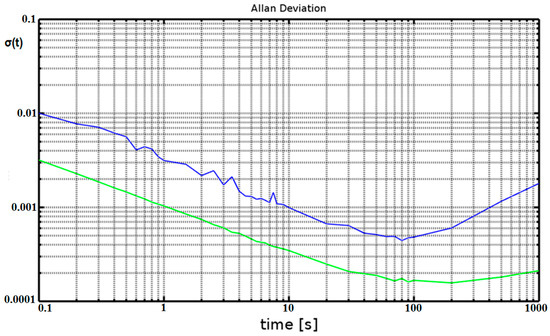
Figure 1.
Accelerometer Allan variance log–log plots of MEMS IMU array (green) vs. single MEMS IMU (blue) [8].
The in-run bias stability standard deviation error references the minima of the Allan deviation curve, as presented in Figure 1 for the data from an IMU array and for a single IMU in static conditions. Using an IMU array is one way to improve accelerometer and gyroscope measurements [6]. The Allan variance is proportional to the total noise power of the sensor output when passed through a bandpass filter. This filter depends on the sampling frequency, and thus, different types of random processes can be examined by adjusting the correlation time. The results for a MEMS gyroscope are similar [12].
The instability of bias drift is the most important measure of the quality of the accelerometer/gyro and is defined as the lowest point on the Allan variance curve, as presented in Figure 1. This is one of the most important parameters for accuracy and overall performance in the context of unassisted inertial navigation [12,14,15].
2.1. Calibration Techniques
The inertial sensor calibration process is a well-defined set of techniques for determining systematic errors [15]. Due to the difference in the set reference value or reference object, it can be divided into two categories—autonomous calibration and non-autonomous calibration [15]. The incremental method proposed in the article can be classified as an autonomous method.
The non-autonomous calibration method is intended for very precise calibration, i.e., the process of comparing the sensor output signal with known reference information and determining coefficients that force the records from the calibrated devices to match the reference records. Usually, this type of calibration is based on large-scale turntables [8]. In this calibration procedure, the bias and scale factor are determined by comparing known parameters to measured output, which is most often implemented in the navigation integration process. This method can be time-consuming and costly, especially if high accuracy is required [16,17].
Autonomous methods, such as equipment-free multi-position-based calibration, are based on the optimization equation that is solved using an iterative weighted least squares correction scheme. However, the autonomous approach requires the computation of the inverse of the matrix. More equations than the number of unknowns should be generated in this case, covering different positions to avoid singularity when computing the inverse of the matrix and obtaining reliable results. Multiple positions means that each wall, side, and corner held vertically up and down is used to provide appropriately different sets of measurements, generated from up to 26 different positions to avoid singularities [14]. Non-autonomous techniques attempt to cover a wide range of inertial calibration schemes but are still not exhaustive of the range of methodologies used. Regarding the standalone calibration method, the use of this method to calibrate a single device has its drawbacks, namely that it requires a specific reference vector, which is difficult to implement in many practical applications. Furthermore, there is no uniform method for detecting multi-sensor calibration errors, especially when it comes to autonomous calibration. The use of different variants of the Kalman filter technique for calibration has not yet been explored well. Additionally, stochastic error models require standardization [18,19]. Nonlinear optimization techniques have evolved into heuristic optimization schemes, which are said to provide a broader search for achieving global optima; however, they have advantages and disadvantages [20,21,22].
To sum up, current calibration techniques do not simultaneously take into account nonlinear scale factors, magnetic disturbances, and g-dependent bias, and no uniform calibration framework is available. MEMS inertial sensors suffer from significant run-to-run biases and thermal drifts, which need to be estimated using infield calibration schemes as these cannot be calibrated in the laboratory setup and are dynamic in nature. Furthermore, the error coefficients also vary with age and environmental conditions, which can be compensated by an infield calibration scheme, and thus, great impetus should be given to improving these techniques. Thus, generally, the scale factor and bias, but not bias drift, can be eliminated by calibration.
The proposed method is an autonomous method but introduces a new incremental approach to determining the bias/errors that accumulate over time.
2.2. Errors Accumulated over Time
There are some types of errors that are still difficult to overcome, i.e., the instability of bias and bias drift [8,12], which refers to the variation in the bias over time caused, for example, by the self-heating of the accelerometer/gyroscope itself and other components of the entire system (both mechanical and electrical). MEMS accelerometers experience drift over time, which affects the accuracy of the measurement (see Figure 2).
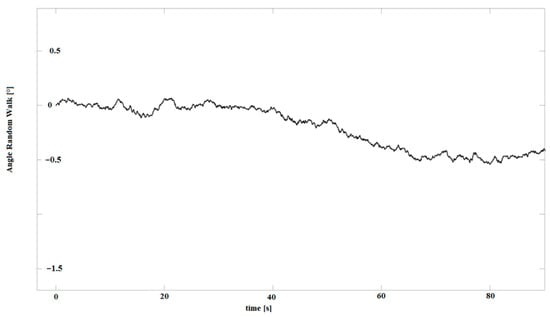
Figure 2.
Angular random walk process records for an Xsens MTi-G-28A53G35 (Xsens, Enschede, The Netherlands) for static measurements.
The velocity, or angular random walk (ARW), is a measure of accelerometer and gyro perturbation by some thermo-mechanical noise, which fluctuates at a rate much greater than the sampling rate of the sensor. This is proportional to the square root of the integration time [5], as presented in Figure 2 for stationary measurements, where the bias error changes with time. The uncertainty of the random walk increases with time, making it a non-stationary process. However, it can be considered stationary within small time intervals [13].
The true vector of a MEMS accelerometer and gyro consists of a vector of accelerometer and a vector of angular rate (AR) :
which, in practice, is:
and relatively:
where:
—acceleration vector.
The variables and represent acceleration and gyro, respectively. The subscripts , , and correspond to the respective axes, while the subscripts , b, and indicate linear, bias error, and noise, respectively.
3. Problem Definition
Due to the problems mentioned above, i.e., ARW and VRW, the process cannot be carried out completely autonomously and passively, and continuous measurement correction is required.
Integrating navigation information involves primarily using Kalman optimal filtering due to the nature of the Kalman filter [23,24,25,26,27,28], as presented in Figure 3. The measurement (innovation) is confronted with the processed measurement from the previous cycle. The cycle or iteration is presented using a feedback loop D (delay); thus, the filtering is essentially the integration of information, as presented in Figure 3 [26].

Figure 3.
Kalman fusion/filtering algorithm.
This approach, shown in Figure 3, is implemented in detail using Algorithm A1 in Appendix A. This algorithm uses the measurement of the acceleration due to gravity to calculate the pitch and roll. The measurement is then corrected with the prediction value using Kalman gain K. This code is the initial step of the proposed algorithm for calculating tilt increments (see Section 4.1. Examples of such systems using the above-mentioned Algorithm A1 or its modifications, e.g., in the form of EKF (extended Kalman filter), is present in IMU sensors as presented Figure 4.

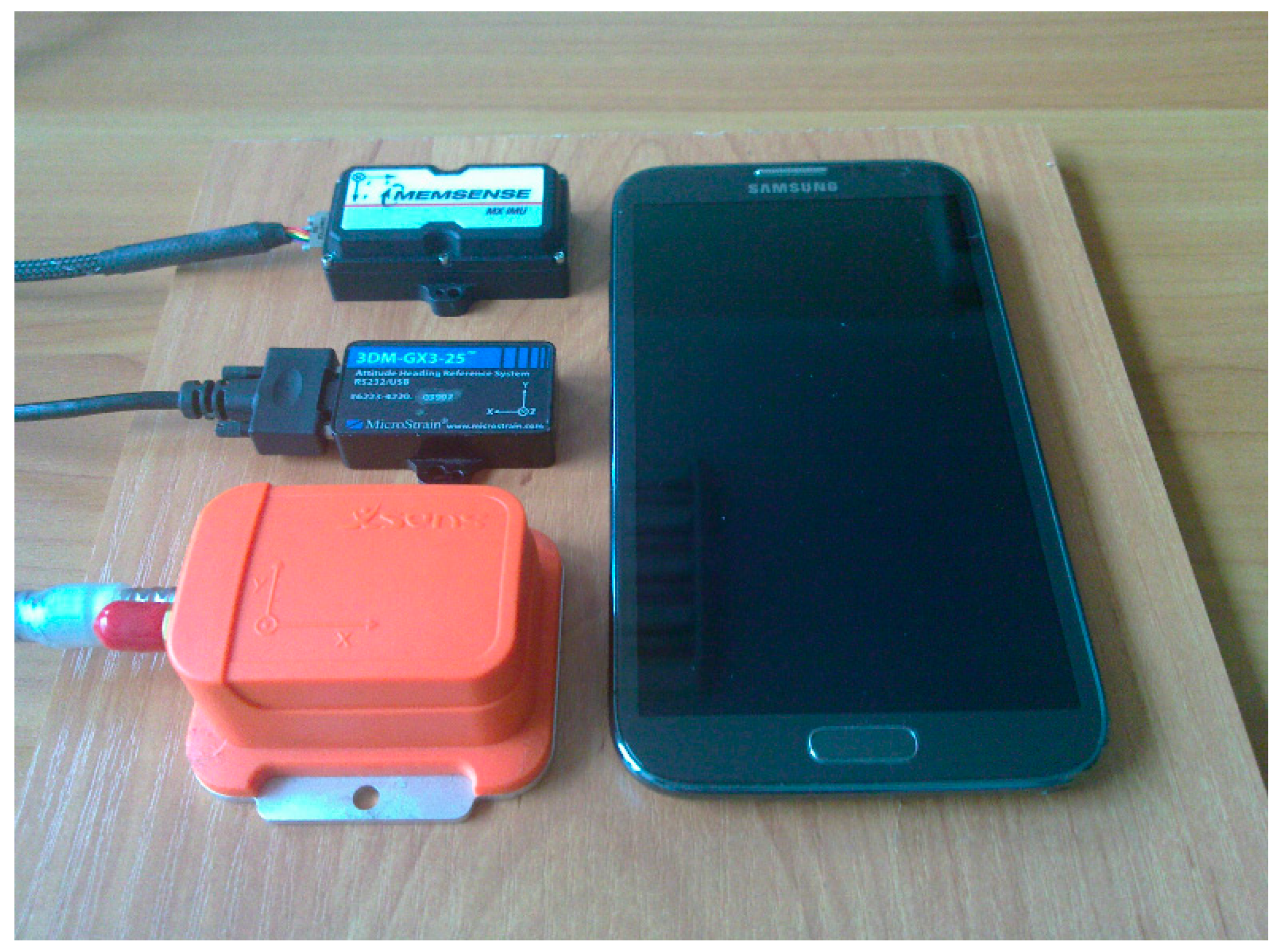
Figure 4.
MEMS Sensors used in the measurement and verification process.
Figure 4 presents MEMS devices from Memsense MX IMU (left top), MicroStrain 3DM-GX3-25 (left middle), Xsens MTi-G-28A53G35 (left bottom), and IMU LSM330 in the form of a Samsung phone (right).
In principle, the error must be removed before taking measurements, but due to its nature and the constantly changing bias error value, calibration must be carried out on an ongoing basis and is most often carried out in the process of fusion or integration of navigation information. Unfortunately, this is difficult due to the principle of equivalence rule.
3.1. Principle of Equivalence as the Main Problem of Inertial Navigation
The principle of equivalence concerns inertial navigation and is a consequence of the principle of relativity resulting from A. Einstein’s general theory of relativity. So far, it has not been possible to demonstrate that the gravitational force due to tilt and the force due to inertia can be distinguished. The equivalence of the force of inertia and the force of gravity shows that the forces of inertia and gravity act on bodies in the same way. This means that if we are under the action of one of these forces, i.e., in the IMU body frame, without an additional source of information, we will not know whether gravity, due to tilt, or inertia is acting on the IMU.
In order to clearly define the problem underlying the operation of inertial sensors, special attention must be paid to the exact distinction between gravitational acceleration due to tilt and linear acceleration. Algorithm A2 in Appendix A illustrates the problem; the algorithm clearly shows that accurate knowledge or measurement of (pitch) and (roll) makes it possible to accurately reconstruct the initial values of linear acceleration , , and . If we had accurate tilt measurements, i.e., pitch and roll, we could eliminate the error in measuring the acceleration of gravity G. Unfortunately, the correction is not easy due to the principle of equivalence because the tilt measurement error and the bias error of the accelerometer readings must be eliminated at the same time.
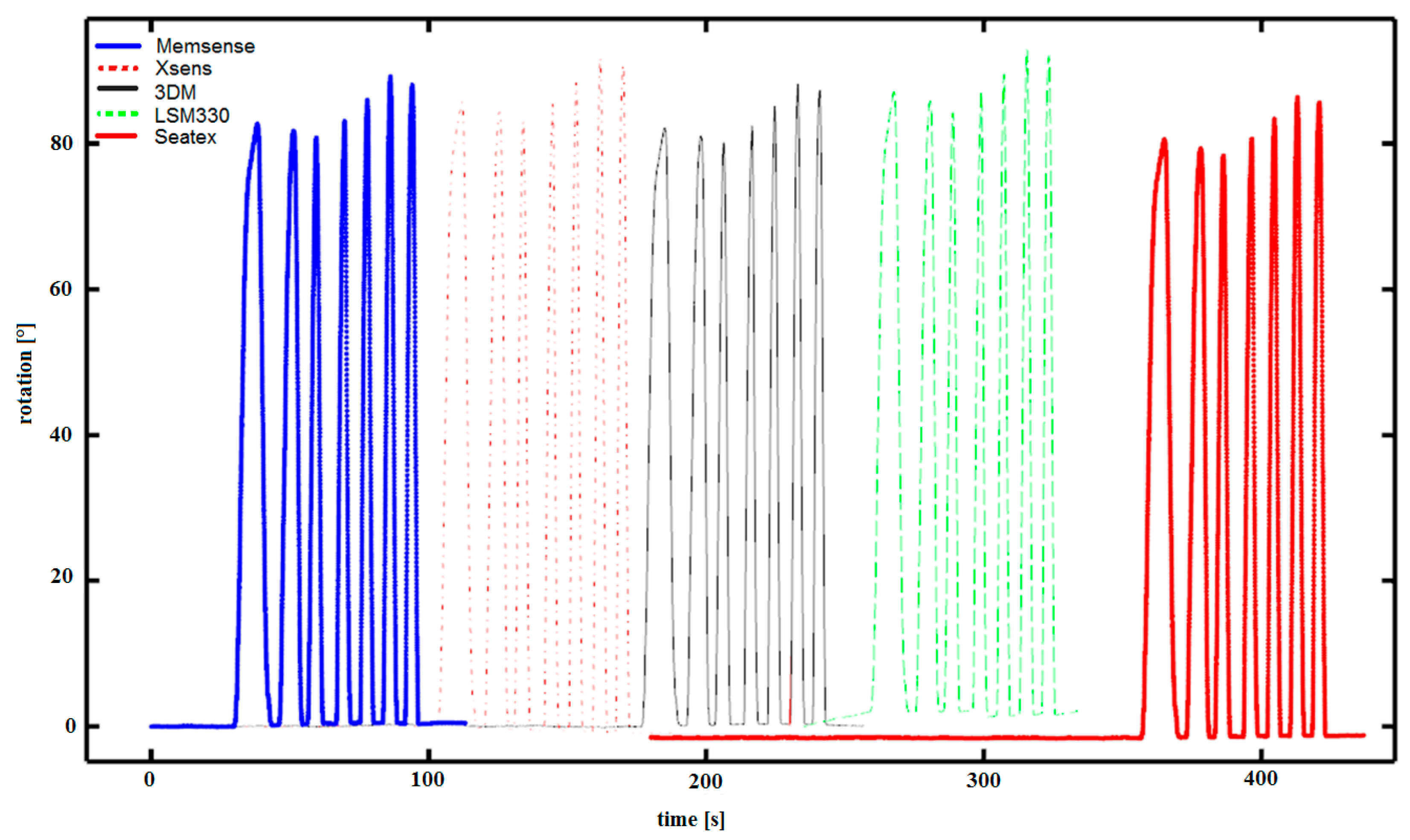
This exact problem affects MEMS chips and IMU devices. As a result, we face a problem that manifests itself in a seemingly minor way, presented in Figure 5: each of the tested IMU devices indicates something different when tilted, which is presented in Figure 6, Figure 7 and Figure 8.
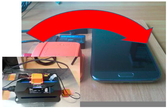
Figure 5.
Set of IMU devices used in measurements.
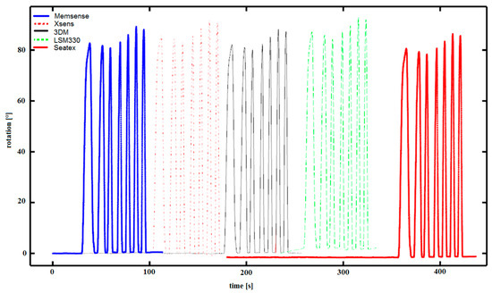
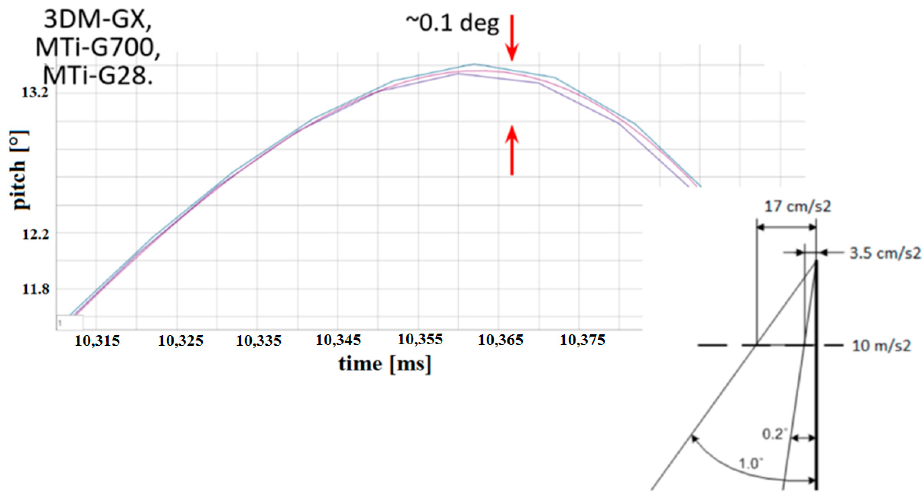
Figure 6.
Records of tilt measurements from Memsense MX IMU, Xsens MTi-G-28A53G35, MicroStrain 3DM-GX3-25, LSM330 IMU, and Seatex MRU IMU-5 Kongsberg.
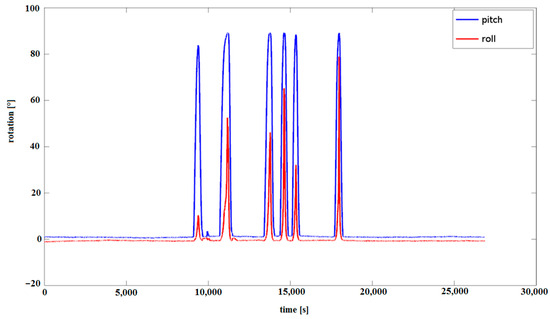
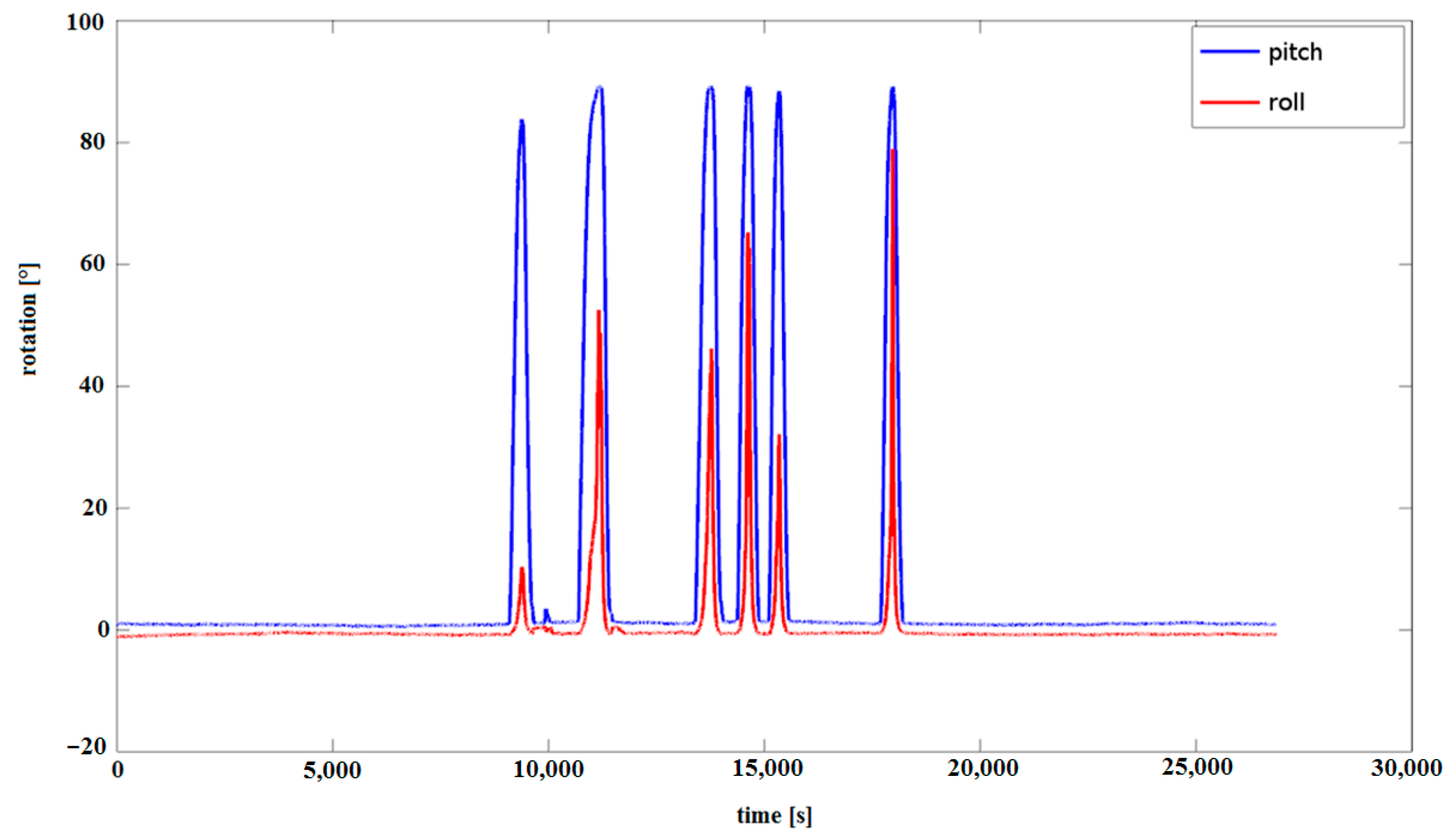
Figure 7.
Tilt measurement of Xsens MTi-G-28A53G35 from Figure 5.
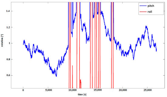
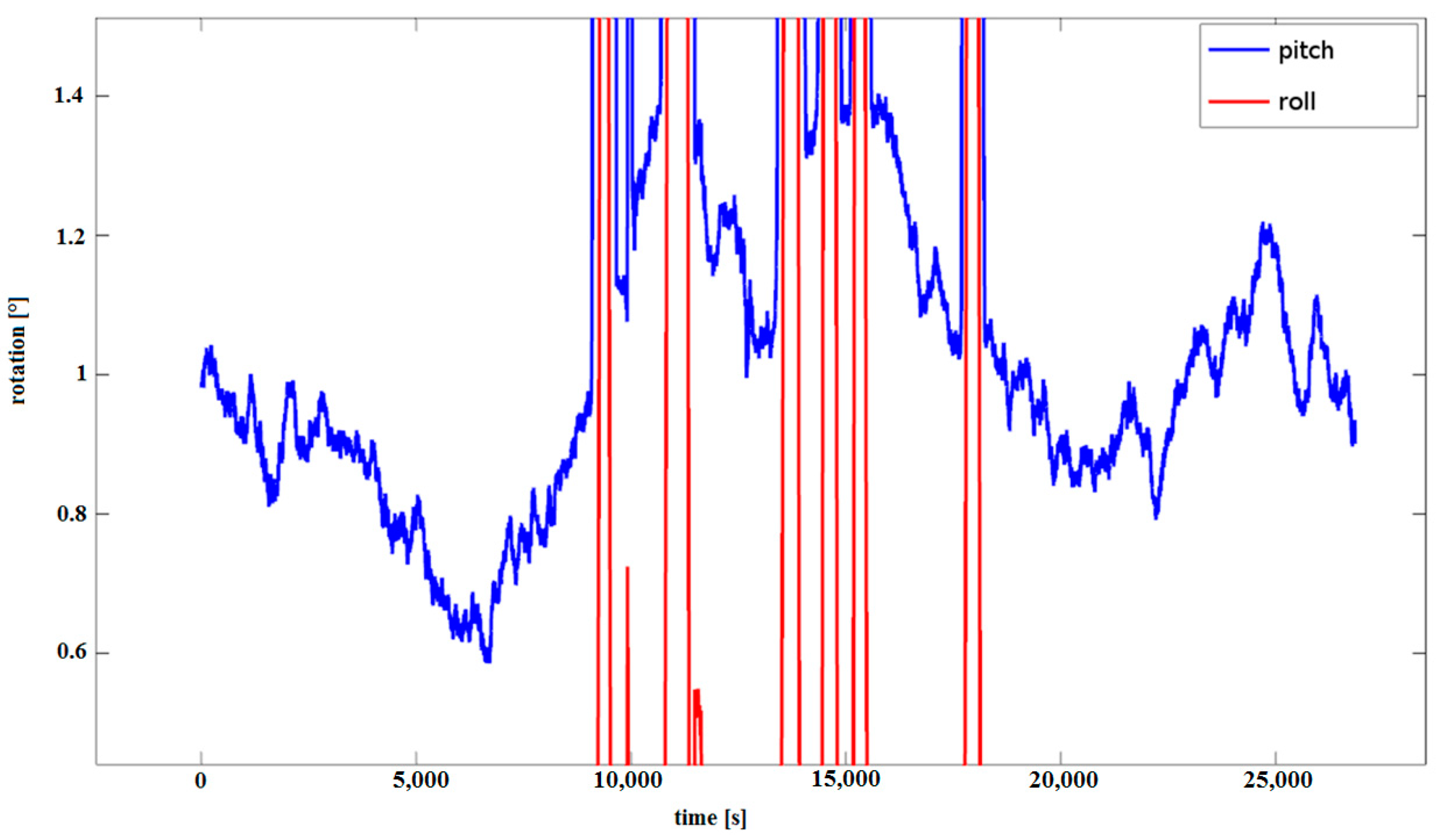
Figure 8.
Tilt measurement of Xsens MTi-G-28A53G35 (pitch enlarged).
This is due to the fact that each device has a different initial error affecting the accelerometer measurements, i.e., when tilted, as in Figure 5, we obtain different initial readings. Figure 5 shows the devices for which simultaneous tilts were performed, i.e., for the Memsense MX IMU (Memsense, Rapid City, SD, USA) [29], Xsens MTi-G-28A53G35 (Xsens, Enschede, The Netherlands) [30] MicroStrain 3DM-GX3-25 (MicroStrain, Williston, ND, USA) [31], and LSM330 IMU (Samsung phone) (STMicroelectronics, Geneva, Switzerland) [32], but also for the high-precision Seatex MRU IMU-5 Kongsberg (Seatex, Rosenberg, TX, USA) [33]; the differences are obvious, as presented in Figure 6.
In Figure 6, differences in measurements can be observed, e.g., for Xsens MTi-G-28A53G35 (red dashed line) and MicroStrain 3DM-GX3-25 (black line). Tilt measurements were performed simultaneously, and the graphs were placed side by side for clarity. Figure 9 shows the same in detail. Similar recorded measurements are presented in Figure 7 for the Xsens MTi-G-28A53G35.
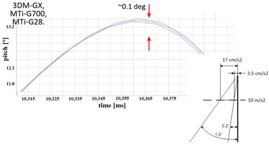
Figure 9.
Differences in roll measurements for the IMUs.
The errors of acceleration may be small, i.e., of the order of 0.001 G; however, they can unfortunately have a significant impact on dead reckoning measurements using the IMU because small differences in tilt measurement result in large errors. Therefore, the tilt measured is similar for all sensors, but there are differences in the shift from the ordinate level to 0, as shown in Figure 6. The actual measurements, as presented in Figure 6, show differences in readings from different IMUs, and even small errors in the tilt IMU measurement have serious consequences in the context of inertial navigation. Figure 7 presents pitch and roll measurements from Xsens MTi-G-28A53G35 using a Kalman filter, and Figure 8 presents the same measurements enlarged for pitch measurements. Despite the use of the Kalman filter, the measurements of pitch are not stable and differ significantly, even in static conditions.
It is enough that the angle measurement system has an error of 0.1 degrees and a linear acceleration error of 0.017 . This is a lot because after 10 s, the error in determining the position will be 1.7 m. This is illustrated in Figure 9. The differences that appear during measurements are presented in detail in Figure 9. Unfortunately, the differences are large. Algorithm 1below shows this using pseudocode.
In dynamic conditions, in the presence of inertial acceleration, readings from the IMU are subject to greater errors.
3.2. Cumulative Error Correction
Algorithm 1 shows that a small change in accelerometer bias error = 0.001 = 0.001 = 0.001 impacts the tilt error measurement = 10.043° and = 30.021°.
Relatively small errors in determining the accelerometer load error = 0.001 = 0.001 = 0.001 causes large errors in tilt calculations. These errors then accumulate in the displacement/navigation calculation process.
| Algorithm 1: Representation of the impact of angle error on overall fusion performance |
| = 10°; = 30°; = 0 ; = 0 ; = 0 ; = 10.000° = 30.000° °; ° = 0.001 G [;=0.001 G ; = 0.001 G []; = 10.043° = 30.021° |
The consequences and results of this simple observation can be presented using well-known calculations resulting from the assumed value of acceleration due to gravity G = 9.81437737 [34]. Even small errors in the tilt measurement have a large impact on the position measurement. Table 2 shows examples of errors in position determination caused only by tilt measurement errors; e.g., for errors of 0.01°, the position error after 10 s is 8.5 cm.
Table 2.
Dead reckoning inertial measurement error due to a lack of tilt compensation.
The point is that the system is not able to give the exact value of tilt and acceleration from gravity without accurate knowledge of pitch and roll, and vice versa; if we knew the exact values of pitch and roll, that is, we knew the exact direct cosine matrix (DCM) values, inertial navigation would become very precise, apart from built-in errors described by the Allan diagram (e.g., angular random walk).
For example, assuming that the bias error for a typical IMU is 0.001 G, then the pitch and roll error will be approximately 0.02–0.04°, which is a lot. For higher-quality accelerometers or, for example, accelerometers that are an order of magnitude better, with a tenfold smaller systematic error or assuming that = 0.001 G = 0.0001 G = 0.0001 G, we observe an improvement of about an order of magnitude = 10.0042827747841°, = 30.0021292279816° (see Algorithm 1). Therefore, taking into account Table 2 above, the error in determining the linear acceleration will be about 0.00034 –0.00068 , respectively. This means that even in the case of such high-class accelerometers, the error is not negligible.
4. Materials and Methods
To partially overcome the problem presented in Section 3.2, a new approach is proposed that exploits the nonlinearity existing between the acceleration value and the sensor tilt , (pitch, roll) and proposes an approach based on the Taylor method, which is presented in Section 4.1 below. This is an incremental method, so the current accelerometer bias error , , and gyroscope deviation error , , , as shown in Equation (5), can be eliminated (by using incremental , measurements).
4.1. New Pitch, Roll, and Accelerometer Bias Estimation Incremental Method
Actual accelerometer measurements also contain bias error, which consists of gravity due to pitch and roll, and random noise, as shown in Equations (4) and (5). Gyroscope errors and accelerometer errors, including random errors, are interdependent and difficult to distinguish.
Assuming linear speed v = 0, , , and , , all equal 0, we can temporarily simplify Equation (4) to
Accelerometer measurement depends on :
where variable represents acceleration of the accelerometer in the accelerometer frame, and represent pitch and roll, respectively, while and are delta pitch and delta roll.
In the above formulas, we use and , which are simply differences (increments) in tilt measurements, i.e., pitch and roll :
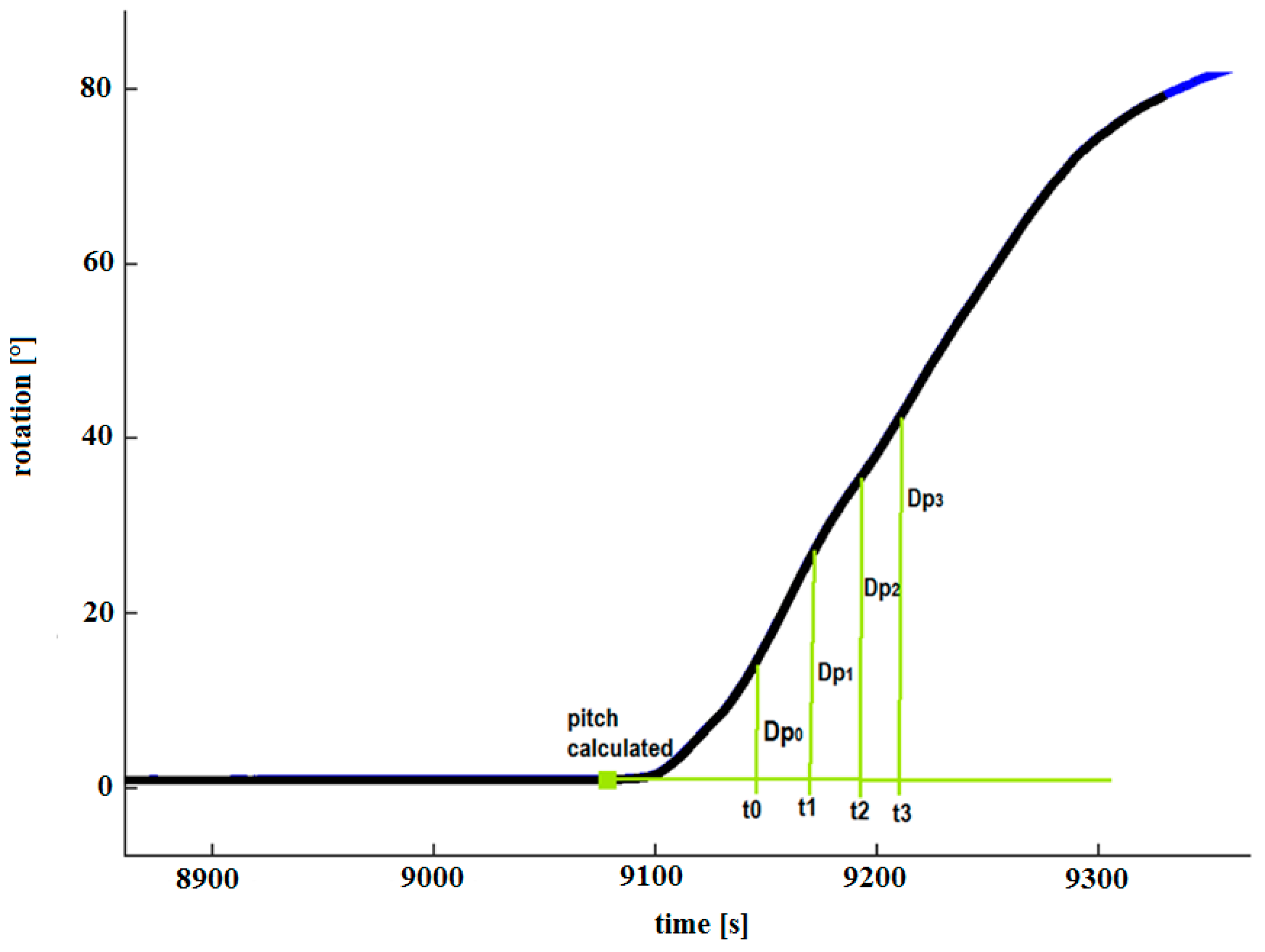
Figure 10 illustrates the idea. Based on , , , , etc. the algorithm calculates .
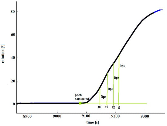
Figure 10.
Differences in roll measurements for the IMUs.
The direct solution to the above equation for ,, ,, is difficult due to the nonlinearity of the above equation (Equation (7)); therefore, Taylor’s differential method was used to solve it, which is briefly presented using the equations below. and can take any values in the range of positive real numbers. In practice, in the range of (0, 90) degrees. We can rewrite Equation (7) in the following form:
where are estimates of real values if . And hence is approximately equal to
Similarly, is approximately equal to
And the same :
Taking into account Equation (8), the derivative of with respect to , is equal to
the derivative of with respect to , equals
Finally, the derivative of with respect to equals
while the derivative of with respect to , equals
the differential
Based on Equation (9), we can write that the estimated and the actual measurement A exist in the following relationship:
where is equal to
while X is equal to
and is a matrix from Equation (22); therefore, we can use the least squares (LSQ) approach to solve the following equation (see Equation (22)):
As a result, , , gives:
and the actual , true equals
4.2. Numerical Example
A working example of the algorithm proposed in Section 4.1 is presented using Algorithm A3 in Appendix A. A demonstration of the proposed algorithm is presented in the form of pseudocode. The state estimator includes the pitch and roll error, and can be initialized using arbitrary scalar values. In subsequent iterations, the actual values are calculated based on measurement (see Equation (9)).
4.3. Algorithm Verification Using Simulation
An important step in creating a new algorithm is its simulation and verification. Algorithms 2 and 3 below make it possible to test Algorithm A3 from Appendix A from different perspectives.
| Algorithm 2: Algorithm test pseudocode representation |
| %initialization = 30; = 10; = 0.005; = 0.002; = 0.003; for i = 1:5 end ; |
As presented in Algorithm 2, above, the only inputs are , i.e., the measurement from the accelerometer, and the difference in the inclination measurement, i.e., and . In response, we obtain the vector :
4.4. Algorithm Verification Using the Side Effect of New Method—Simulation
Due to the nature of the proposed algorithm, an additional property of the proposed algorithm was obtained. The and matrices can be of any size , with . This property gives rise to an interesting but relatively positive property of this algorithm. As is known, typical waveforms for MEMS acceleration sensors may be subject to random errors, as shown in Figure 2, Figure 7, and Figure 8. We know from the theory of measurement systems [8,16] that the sum of parallel measurements is always better than a single measurement.
The procedure detailed below tests the new algorithm in the presence of such random disturbances. Noise was introduced or added to prove this. Matrix A can have any dimension , where . A slight modification to Algorithm 2 confirms that an additional benefit can be achieved by using a larger number of measurements, i.e., from a larger vector of size .
The algorithm modified in this respect is presented as Algorithm 3. In the presented algorithm, represents Gaussian noise.
| Algorithm 3: Proposed algorithm’s side effect test pseudocode representation |
| for j = 1:1000 %add random noise = 30°; = 10°; = = 0.002 + ; = 0.003 + ; for i = 1:5 end end |
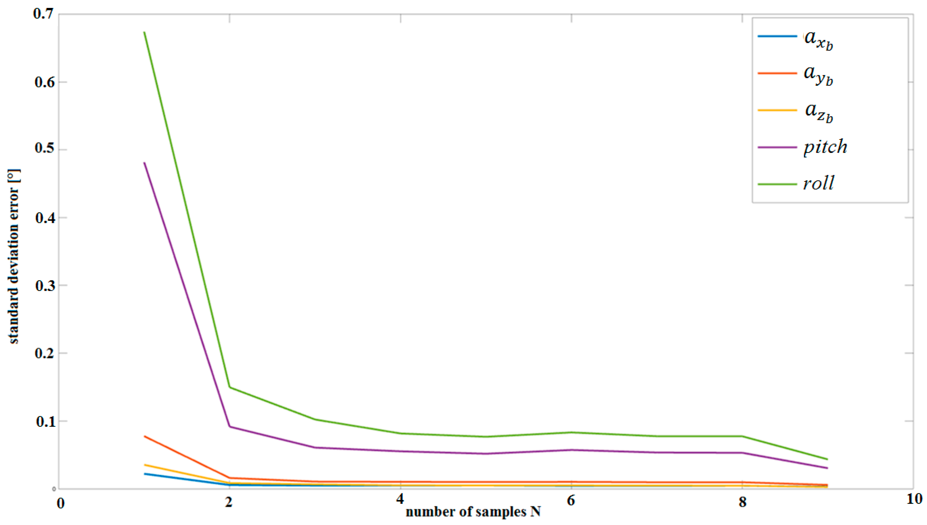
Table 3 presents a summary of the values of the standard deviation, i.e., standard deviations calculated for different values of N.
Table 3.
Standard errors vs. samples N.
Table 3 shows the results of standard deviations for different numbers N of measurements. The results of the calculations were obtained in conditions close to real ones.
As can be easily seen in Figure 11, as the number of measurements N increases, i.e., the number of equations in Equation (22), the accuracy of pitch, roll, and bias error (,, , ) measurements improves. This is a positive effect that characterizes the LSQ approach.
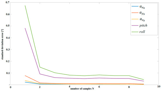
Figure 11.
Standard deviation versus number of measurement samples N for pitch, roll, and bias errors.
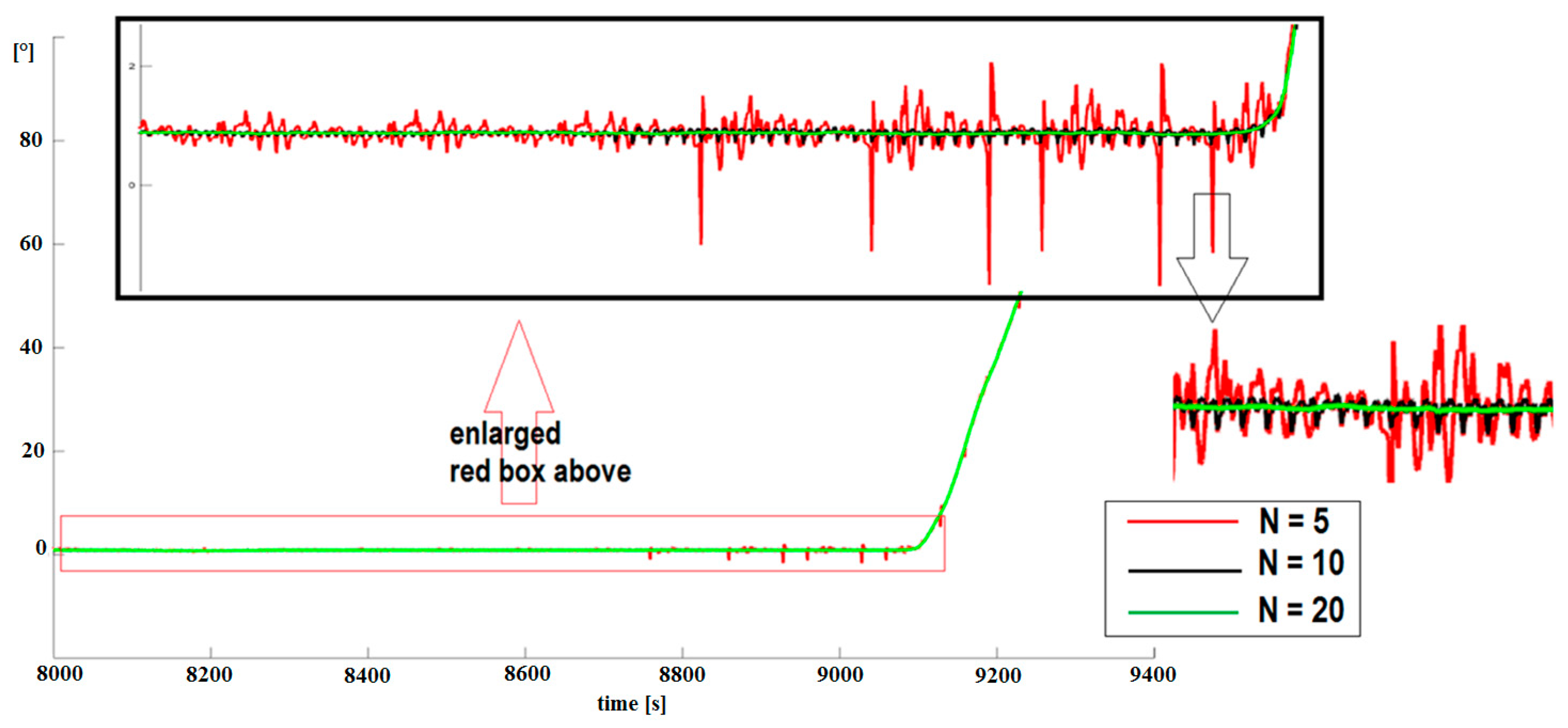
The application of the proposed algorithm to real data from MEMS Xsens MTi-G-28A53G35 confirms the simulations performed. Figure 12 shows the effect of using the algorithm described in Section 4.1 for different N = 2 (green), N = 10 (black), and N = 20 (green). The green figures give the best results and confirm the simulations. Figure 12 presents pitch measurements for different N. Quality improves as N increases (real records).
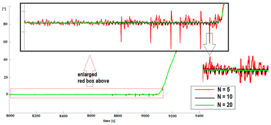
Figure 12.
Pitch measurement for different N. Quality improves as N increases (real records).
5. Results
The algorithm was tested for the Xsens MTi-G-28A53G35 MEMS sensor because this MEMS sensor has good angle ratio (AR) bias performance, as presented in Figure 2. The algorithm was also tested for the Xsens MTi-G-28A53G35 sensor because it has an implemented EKF filter and, in practice, gives better pitch and roll records [16], as shown in Figure 13.
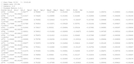
Figure 13.
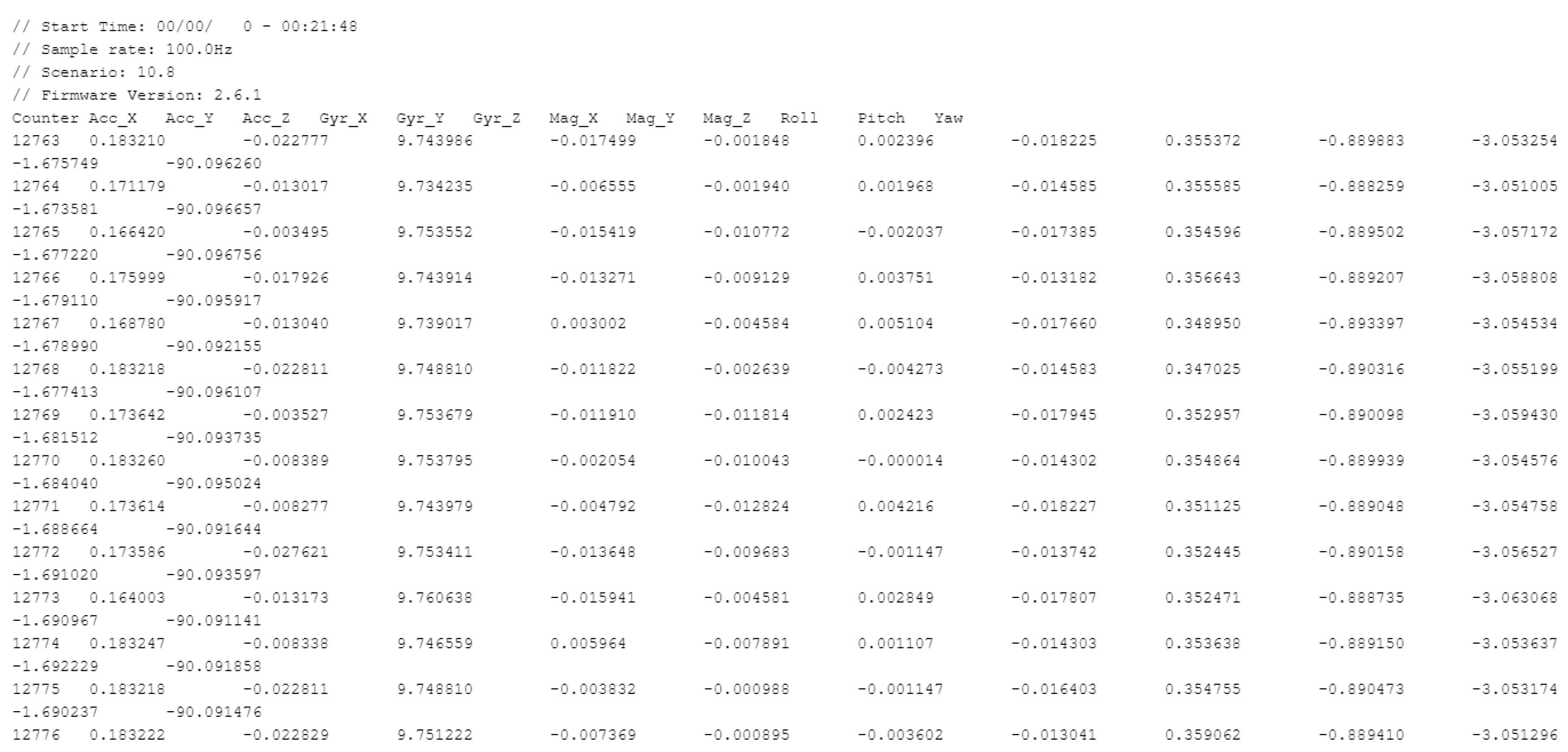
Xsens MTi-G-28A53G35 record samples.
Record samples from the Xsens MEMS MTi-G-28A53G35 are presented in Figure 13. Columns 2–4 are the accelerometer measurements, columns 5–7 are the gyro angular rate (AR), and columns 10–12 are the roll, pitch, and yaw. The last columns are the result or output of the EKF filter implemented in this device [16].
Integration of Proposed Algorithm with Kalman Sensor Fusion Algorithm
Algorithm A4 from Appendix A shows the process of integrating both algorithms into a combined final algorithm that simultaneously combines/integrates measurements from gyroscopic sensors and accelerometers and corrects the initial pitch, roll, and accelerometer bias error values.
The integration of these algorithms is very simple and perhaps requires further research, at least in terms of better integration. The actual pitch and roll values are corrected by correctly calculated bias errors, i.e., , , , after the “read Xsens MEMS sensor , , ” line of the Algorithm A4 from Appendix A.
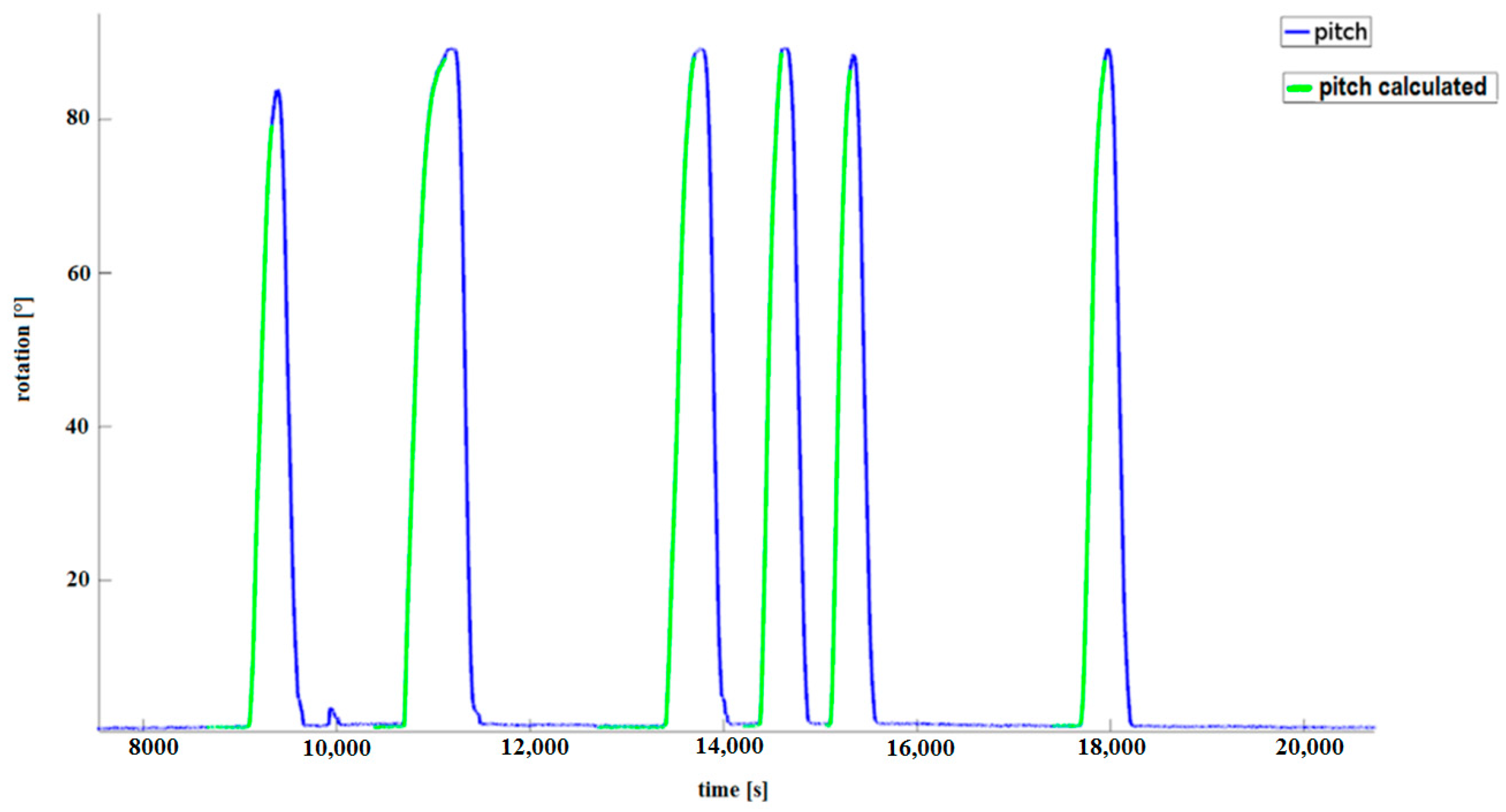
Figure 14 shows the results of applying this algorithm to the raw records. Measurements from the built-in EKF algorithm in the IMU MTi-G-28A53G35 are presented in blue, i.e., column 11 of the recorded data from the IMU MTi-G-28A53G35 (see Figure 13).
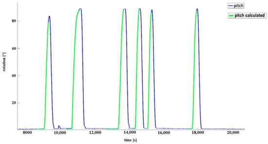
Figure 14.
Result of pitch measurements using IMU MTi-G-28A53G35. The fragment marked with green color represents tilt using the proposed algorithm. The fragment is enlarged in Figure 15.
The green line (pitch) presents the results of pitch measurements using the proposed algorithm (see Figure 14); the figure presents the results of the estimated pitch using Kalman (blue) and pitch calculated using the proposed algorithm (green).
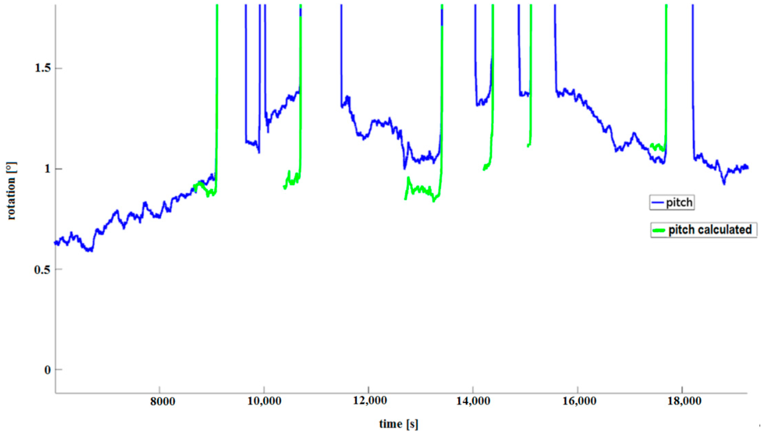
Figure 15 presents some details of Figure 14. If we look closer at the measurement record in Figure 15, it can be seen that there are differences in the pitch measurements both recorded and calculated using Algorithm A4 (pitch in green color), and using the algorithm built into the MTi-G-28A53G35 (pitch Xsens in blue color, evaluated using the Kalman algorithm). The standard errors for these pitch measurements are presented in Table 4. This is not surprising if we recall the visualizations in Figure 2, where the gyro accumulated errors are presented and discussed for measurements carried out. An example of a array looks like this:
i.e., 13 increments of . A high dynamics of increments was assumed, from approx. 0 to 80°. It should be emphasized here that the algorithm is suitable for dynamic conditions. Table 4 presents standard errors of measurements for the proposed algorithm and the Kalman algorithm. The proposed algorithm gives much better results.
Dp = [5.0227;11.1731;17.4920;23.5077;29.4961;35.4627;41.4013;47.3563;53.3220;59.3947;65.4093;71.4177;77.3618]°
Figure 15.
Detailed result of pitch measurements using the IMU MTi-G-28A53G35.
Table 4.
Standard errors of measurements for the proposed algorithm and the Kalman algorithm.
A test similar to the tests carried out in Algorithm 2 was also performed. Therefore, if we introduce an artificial disturbance into the input data, e.g., to the second column of Figure 13 (the acceleration value ), by adding any disturbance in the form of, e.g., = 0.01 , to the value of this bias error, it will be recalculated correctly with an accuracy of 0.0001 . However, this accuracy depends on the value of the bias error introduced and decreases as it increases, i.e., for bias error of = 0.06 , the accuracy of the estimation is about 0.01 . This means that the system can be calibrated quite precisely under dynamic conditions.
6. Discussion and Conclusions
The article presents a modified method for determining the initial values of pitch, roll, and acceleration using incremental (differential) pitch and roll measurements. Therefore, a difference in tilt (not a tilt) measurements is required, which can be considered an innovation. The paper presents a detailed theoretical justification of the proposed method, which is based on the derivatives approach to nonlinear equations. It improves the determination of IMU MTi-G-28A53G35 tilt (i.e., pitch and roll) to 0.001° even under dynamic pitch/roll conditions (autonomous method), which is a significant improvement as it makes it possible to determine the position using the dead reckoning method from the IMU system, with an accuracy of approximately 0.2 cm per 10 s (Table 2). The individual parts of the article present detailed implementations of this method, as well as tests on simulated and real data from various IMUs, especially the MTi-G-28A53G35 sensor.
Gyro measurements (AR) do not depend on linear acceleration and gravity, and the proposed method exploits this feature. The most important part of the article and at the same time the most important part of the proposed method is presented in paragraph 4.1, while verification of this method is presented in Section 4.2, Section 4.3 and Section 4.4. The algorithm has a solid mathematical foundation, as presented in Section 4.1, and has been tested on real, recorded and simulated/synthetic data. The integration of the proposed algorithm with the optimization–integration filter, i.e., the Kalman fusion filter, is presented in the form of Algorithm A4 in Appendix A. Although this is an effective integration, it is not a perfect approach, so the next step will be to look into better Kalman-proposed method integration. Further research for better integration and improved implementation of Algorithm A4 may be necessary due to its superior practical applications. Thus, attempts at integration with EKF filters and further research in this direction will be carried out. It is worth recalling another important problem at this point, which is the stability of pitch and roll measurements due to random walk (ARW), i.e., the calculations of tilt and bias error; thus, , , , , , will only be valid for a certain period of time, because the method uses incremental measurements of tilt. This is natural for ARW processes and justifies the usage of the proposed algorithm.
Finally, it is worth emphasizing that the algorithm uses gravitational acceleration G. In the calculations, gravity is assumed to be G = 9.81437737 . The precision of the results obtained using the proposed algorithm requires an accurate determination of G for a given location on Earth.
Funding
This research received no external funding.
Data Availability Statement
The data presented in this study are available on request from the corresponding author.
Conflicts of Interest
The author declares no conflict of interest.
Appendix A
| Algorithm A1: Pseudocode representation of the Kalman filter fusion process |
| for i = start to end end |
Algorithm A1 uses a well-known version of the notation typically used in the implementation of the Kalman filter, but for completeness, the notation is as follows [15]:
- —estimation vector:
- —covariance of the observation noise (uncertainty of the measurement).
- —covariance of the process noise (uncertainty of the system model).
- —Kalman gain.
- —estimate covariance matrix (uncertainty of the state estimate).
| Algorithm A2: Pseudocode linear acceleration definition |
| //set North–East–Down vector and linear acceleration LinNoG NED = ; LinNoG = //random roll and pitch = randn(1); = randn(1); //direct cosine matrix for roll and pitch DCM = Euler2DCM( × deg2rad, × deg2rad, 0); BiasFromG = DCM × NED; //overall acceleration = BiasFromG + DCM × ; //reverse operation, calculate acceleration in MEMS framework NoG = ( − DCM × NED); //calculate above linear acceleration, inverse operation LinNoG = = inv(DCM) × ( − DCM × NED); |
- NED—North–East–Down framework;
- DCM—direct cosine matrix;
- deg2rad = pi/180;
- rad2deg = 180/pi;
- LinNoG—linear acceleration without gravitational component (may be biased).
| Algorithm A3: Pseudocode representation of the proposed algorithm |
| function = asolve_bias(, ,, ) |
| Algorithm A4: Pseudocode representation of integration of the proposed algorithm and Kalman algorithm |
| Initialize , , and //uncertainty of the state estimate //uncertainty of the system model //uncertainty of the measurement for i = start to :end read Xsens MEMS sensor , , %%%%%%%%%%%%%%%%%%integration with asolve_bias from Algorithm 3 for i = 1:5 end ; End |
References
- Paull, L.; Saeedi, S.; Seto, M.; Li, H. AUV Navigation and Localization: A Review. IEEE J. Ocean. Eng. 2014, 39, 131–149. [Google Scholar] [CrossRef]
- Demkowicz, J. Autonomous Vehicle Navigation in Dense Urban Area in Global Positioning Context. In Proceedings of the 2018 11th International Conference on Human System Interaction (HSI), Gdansk, Poland, 4–6 July 2018. [Google Scholar]
- ASG-EUPOS. EUPOS, System Description. Reference Stations. Available online: http://www.asgeupos.pl/ (accessed on 17 February 2024).
- Yeong, J.; Velasco-Hernandez, G.; Barry, J.; Walsh, J. Sensor and Sensor Fusion Technology in Autonomous Vehicles: A Review. Sensors 2021, 21, 2140. [Google Scholar] [CrossRef]
- Groves, P.D. Principles of GNSS, Inertial, and Multisensor Integrated Navigation Systems; Artech House: London, UK, 2013. [Google Scholar]
- Kaplan, E.D.; Hegarty, C.J. Understanding GPS/GNSS Principles and Applications; Artech House: London, UK, 2017. [Google Scholar]
- Woodman, O.J. An Introduction to Inertial Navigation; University of Cambridge: Cambridge, UK, 2007. [Google Scholar]
- Demkowicz, J.; Bikonis, K. Study of Array of MEMS Inertial Measurements Units Under Quasi-Stationary and Dynamic Conditions. Pol. Marit. Res. 2021, 28, 150–155. [Google Scholar] [CrossRef]
- Demkowicz, J.; Bikonis, K. MEMS Technology Quality Requirements as Applied to Multibeam Echosounder. Pol. Marit. Res. 2018, 25, 59–64. [Google Scholar]
- Kovacic, I.; Brennan, M.J. The Duffing Equation: Nonlinear Oscillators and Their Behaviour; John Wiley & Sons: Hoboken, NJ, USA, 2011. [Google Scholar] [CrossRef]
- Azizi, T.; Kerr, G. Application of Stability Theory in Study of Local Dynamics of Nonlinear Systems. J. Appl. Math. Phys. 2020, 8, 1180–1192. [Google Scholar] [CrossRef]
- Quinchia, A.G.; Falco, G.; Falletti, E.; Dovis, F.; Ferrer, C. A Comparison between Different Error Modeling of MEMS Applied to GPS/INS Integrated Systems. Sensors 2013, 13, 9549–9588. [Google Scholar] [CrossRef] [PubMed]
- Demkowicz, J. MEMS Gyro in the Context of Inertial Positioning. In Proceedings of the 2017 Baltic Geodetic Congress (BGC Geomatics), Gdansk, Poland, 22–25 June 2017; pp. 247–251. [Google Scholar]
- Poddar, S.; Kumar, V.; Kumar, A. A comprehensive overview of inertial sensor calibration techniques. J. Dyn. Syst. Meas. Control 2017, 139, 011006. [Google Scholar] [CrossRef]
- Ru, X.; Gu, N.; Shang, H.; Zhang, H. MEMS Inertial Sensor Calibration Technology: Current Status and Future Trends. Micromachines 2022, 13, 879. [Google Scholar] [CrossRef] [PubMed]
- Aggarwal, P.; Syed, Z.; Niu, X.; El-Sheimy, N. A Standard Testing and Calibration Procedure for Low Cost MEMS Inertial Sensors and Units. J. Navig. 2008, 61, 323–336. [Google Scholar] [CrossRef]
- Syed, Z.; Aggarwal, P.; Goodall, C.; Niu, X.; El-Sheimy, N. A New Multi-Position Calibration Method for MEMS Inertial Navigation Systems. Meas. Sci. Technol. 2007, 18, 1897–1907. [Google Scholar] [CrossRef]
- Bekkeng, J.K. Calibration of a Novel MEMS Inertial Reference Unit. IEEE Trans. Instrum. Meas. 2009, 58, 1967–1974. [Google Scholar] [CrossRef]
- Wang, B.; Ren, Q.; Deng, Z.; Fu, M. A Self-Calibration Method for Nonorthogonal Angles Between Gimbals of Rotational Inertial Navigation System. IEEE Trans. Ind. Electron. 2015, 62, 2353–2362. [Google Scholar] [CrossRef]
- Łuczak, S.; Zams, M.; Dabrowski, B.; Kusznierewicz, Z. Tilt Sensor with Recalibration Feature Based on MEMS Accelerometer. Sensors 2022, 22, 1504. [Google Scholar] [CrossRef] [PubMed]
- IEEE Recommended Practice for Inertial Sensor Test Equipment Instrumentation Data Acquisition and Analysis. Available online: https://ieeexplore.ieee.org/servlet/opac?punumber=10423 (accessed on 31 March 2011).
- Dong, X.; Huang, X.; Du, G.; Huang, Q.; Huang, Y.; Huang, Y.; Lai, P. Calibration Method of Accelerometer Based on Rotation Principle Using Double Turntable Centrifuge. Micromachines 2022, 13, 62. [Google Scholar] [CrossRef] [PubMed]
- Anderson, B.D.O.; Moore, J.B. Optimal Filtering; Dover Books on Electrical Engineering; Courier Corporation: North Chelmsford, MA, USA, 2005. [Google Scholar]
- Brown, R.G.; Hwang, P.Y.C. Introduction to Random Signals and Applied Kalman Filtering with MATLAB Exercises, 3rd ed.; John Wiley & Sons Inc.: New York, NY, USA, 1997. [Google Scholar]
- Abdolkarimi, E.S.; Mosavi, M.R. A low-cost integrated MEMS-based INS/GPS vehicle navigation system with challenging conditions based on an optimized IT2FNN in occluded environments. GPS Solut. 2020, 24, 108. [Google Scholar] [CrossRef]
- Sayed, A.H. Adaptive Filters; John Wiley & Sons, Inc.: Hoboken, NJ, USA, 2008. [Google Scholar]
- IEEE Std 952-1997; IEEE Standard Specification Format Guide and Test Procedure for Single-Axis Interferometric Fiber Optic Gyros. IEEE: New York, NY, USA, 1998.
- Shultz Kenneth, S. Measurement Theory in Action; Taylor & Francis Ltd.: Abingdon, UK, 2020. [Google Scholar]
- MX IMU Product Specification & User Guide Document Number: DOC00295 Document Revision: E MEMSENSE.COM 888.668.8743, USA. Available online: https://www.memsense.com/assets/docs/uploads//mx/DOC00295_Rev-D_MX-IMU_PSUG.pdf (accessed on 29 July 2024).
- MTi-G User Manual and Technical Documentation, Xsens Technologies B.V., France. Available online: https://www.movella.com/products/xsens (accessed on 23 December 2023).
- Quick Start Guide to the 3DMGX3 Soft & Hard Iron Calibration. Available online: https://www.microstrain.com (accessed on 17 February 2024).
- LSM330DLC, iNEMO Inertial Module, 3-axis Accelerometer and 3-axis Gyroscope, Data Sheet, STMicroelectronics. 2016. Available online: https://www.st.com/resource/en/datasheet/dm00037200.pdf (accessed on 29 July 2024).
- Kongsberg Seatex MRU-5 Manual, Copyright© Kongsberg Seatex AS. 2008, Norway. Available online: http://linux.geodatapub.com/shipwebpages/survey%20gear/Multibeam/EM1002%20-%20Powell/manuals/mru%20and%20h%20install%20manual.pdf (accessed on 29 July 2024).
- Sas-Uhrynowski, A. Absolute Gravity Measurements in Poland; Cartography Monographic Series; Institute of Geodesy: Warsaw, Poland, 2002; ISBN 83-916216-2-6. Available online: http://bc.igik.edu.pl/Content/30/PDF/SM_3_15028_8391621626.pdf (accessed on 17 February 2024).

Disclaimer/Publisher’s Note: The statements, opinions and data contained in all publications are solely those of the individual author(s) and contributor(s) and not of MDPI and/or the editor(s). MDPI and/or the editor(s) disclaim responsibility for any injury to people or property resulting from any ideas, methods, instructions or products referred to in the content. |
© 2024 by the author. Licensee MDPI, Basel, Switzerland. This article is an open access article distributed under the terms and conditions of the Creative Commons Attribution (CC BY) license (https://creativecommons.org/licenses/by/4.0/).