Aerial SfM–MVS Visualization of Surface Deformation along Folds during the 2024 Noto Peninsula Earthquake (Mw7.5)

Abstract

This study aimed to map and analyze the spatial pattern of the surface deformation associated with the 2024 Noto Peninsula earthquake (Mw7.5) using structure-from-motion/multi-view-stereo (SfM–MVS), an advanced photogrammetric technique. The analysis was conducted using digital aerial photographs with a ground pixel dimension of 0.2 m (captured the day after the earthquake). Horizontal locations of GCPs were determined using pre-earthquake data to remove the wide-area horizontal crustal deformation component. The elevations of the GCPs were corrected by incorporating quasi-vertical values derived from a 2.5-dimensional analysis of synthetic aperture radar (SAR) results. In the synclinorium structure area, where no active fault had previously been identified, we observed a 5 km long uplift zone (0.1 to 0.2 km in width), along with multiple scarps that reached a maximum height of 2.2 m. The area and shape of the surface deformation suggested that the induced uplift and surrounding landslides were related to fold structures and their growth. Thus, our study shows the efficacy of SfM–MVS with respect to accurately mapping earthquake-induced deformations, providing crucial data for understanding seismic activity and informing disaster-response strategies.

1. Introduction

On 1 January 2024, a moment magnitude 7.5 earthquake, known as the 2024 Noto Peninsula earthquake, occurred in the Noto Peninsula (Ishikawa Prefecture) at a depth of 16 km (Figure 1b) along the Sea of Japan coast of Honshu, Japan. With respect to- the seismogenic mechanism, the earthquake was a reverse fault type with a northwest–southeast compressive axis [1], with the source fault estimated to be mainly southeast-trending and extending northeast–southwest for approximately 150 km [2]. Analysis of synthetic aperture radar (SAR) images from the Advanced Land Observing Satellite-2 (ALOS) “Daichi-2” revealed maximum uplift and westward variation of approximately 4 and 2 m, respectively, in the western part of Wajima City. In comparison, the corresponding values in the northern part of Suzu City were approximately 2 and 3 m, respectively (Figure 1a) [3]. On the seafloor off the Noto Peninsula, several southeast-trending reverse faults have been identified as active, and these extend mainly northeast–southwest from the offshore west of the Noto Peninsula to areas north and northeast [4,5]. This active fault was estimated to be most likely associated with the earthquake [2], resulting in the observed uplift of the seafloor topography at multiple locations [6,7].

Terrestrial surface deformation was investigated using structure-from-motion/multi-view-stereo (SfM–MVS). Previous studies on surface deformation analysis using SfM–MVS have focused on detailed fault topography analysis using an Unmanned Aerial Vehicle (UAV) [10,11] and detection of displacement caused by past earthquakes [12,13]. The SfM–MVS of the Noto Peninsula earthquake used aerial photography by a manned aircraft as an emergency response. This SfM–MVS study focuses on easily and rapidly identifying surface deformation in the event of a widespread disaster. Aerial photographs captured by the Geospatial Information Authority of Japan (GSI) on January 2, 2024 were utilized to generate post-earthquake digital surface models (DSMs). Additionally, DSMs were generated from light detection and ranging (LiDAR) 3D point clouds obtained before the earthquake and analyzed using the digital elevation model (DEM) of difference (DoD) before and after the earthquake. Consequently, a 4 km-long strip of surface deformation with a maximum vertical displacement of approximately 2 m was observed along the Wakayama River in Suzu City, Ishikawa Prefecture, northeast of the Noto Peninsula [14]. Topographic measurements were further supplemented by field surveys [15,16]. Previous pre-earthquake geological and variable geomorphological studies [9,17,18] did not identify any active faults along the Wakayama River, with synclines and anticlines constituting the synclinorium structure known to be distributed parallel to the Wakayama River [9,17]. A prompt understanding of the location and magnitude of permanent topographic deformation during earthquakes is crucial for rapidly responding to infrastructure damage, predicting the locations of zones susceptible to surface deformation, and conducting effective hazard analysis during seismic events. This study builds on the methodology proposed by Yoshida [14], which was initially presented in a preliminary report. It provides a detailed account of the survey methodology and presents the analysis results of surface deformation along the Wakayama River, observed using SfM–MVS immediately following the earthquake.

2. Survey

Interpretation of aerial photographs taken by the GSI on 2 January 2024 revealed linear surface deformation in the Naka area, Wakayama Town, Suzu City, Ishikawa Prefecture, Japan. In this study, the study area was set to cover an area larger than the initial surface-deformation area, and the SfM–MVS analysis was conducted using aerial photographs. The analysis area extended approximately 11 km from east to west and 8 km from north to south (Figure 2).

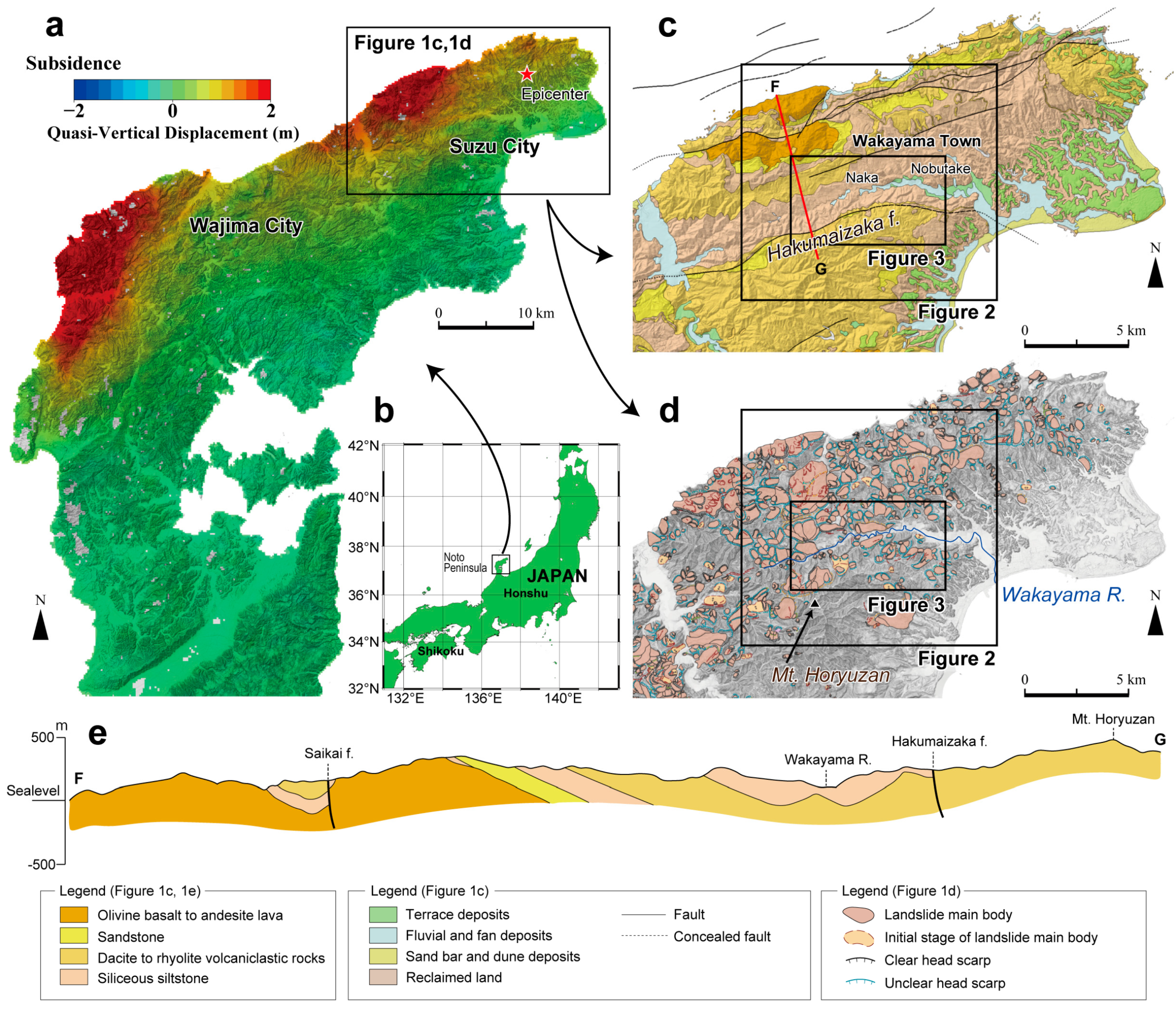
2.1. Geology

An overview of the geology of the area, based on a study by Yoshikawa et al. [9], is provided below. In the northeastern part of the Noto Peninsula, geological strata formed approximately 30 million years ago are distributed (Figure 1c). These geological formations fold in a northeast–southwest to east–west direction and are cut by faults in the same direction. Notably, the Hakumaizaka Fault [17], located south of the Wakayama River area, is a reverse fault with significant displacement. The geological structure, distribution, and thickness of these formations differ greatly between their southern and northern sides. The surface deformation observed in this study is located north of the Hakumaizaka Fault, where numerous folds and reverse faults cut through the northern wing of the anticline, with a synclinorium structure evident around the Wakayama River.

2.2. Geomorphology

The region’s highest peak, Mt. Horyuzan (468.5 m above sea level), is located in the southwest. Numerous old landslide landforms exist on the slopes of these hills (Figure 1d). Geological structures and rock formations influence the course of many river channels in the upper reaches of the Wakayama River, which flow along synclinorium structures. The Wakayama River shows incised meanders with significant sinuosity and various river-capture landforms distributed along its course.

3. Materials and Methods

The linear surface deformation was identified through naked-eye stereoscopic visual inspection using aerial photographs captured by the GSI on 2 January 2024. DEMs of difference (DoDs) diagrams were created from pre- and post-earthquake numerical elevation models to illustrate the spatial distribution of vertical displacement, thereby enhancing the identification and correction of locations exhibiting linear surface deformation. In addition, feature points were extracted from pre- and post-earthquake orthoimages to determine horizontal displacement. Notably, the paddy-field plots in this area have been artificially modified through land-improvement projects since the 1970s. Therefore, digital surface models (DSMs) were generated from aerial photographs taken in the 1960s, before human alteration, to explore potential correlations between surface deformation and DSMs.

3.1. Pre-Earthquake DTM (2022DTM)

A digital terrain model (DTM) with a resolution of 0.5 m (Japan Plane Rectangular Coordinate System 7; EPSG: 6675), derived from the 2024 Noto Peninsula Earthquake (DEM before the Noto East Earthquake), was used. This DTM was created and published by Asahi Koyo Corporation and was based on 3D point cloud data (LAS format) from the 2022 Forest Information Maintenance Work conducted by Ishikawa Prefecture between August and October 2022. The absolute accuracy (RMSE) of the height is within 0.3 m.

3.2. Post-Earthquake DSM (2024DSM)

The DSM was produced by SfM–MVS analysis using 24 aerial photographs (ground pixel dimension of approximately 0.2 m; JPEG format) of the study area in the Suzu region, taken by the GSI on 2 January 2024. The aerial photographs were taken at 4650 m above ground level with a resolution of 14,592 × 25,728 pixels. The overlap and side-lap ratios of the images were approximately 65% and 35%, respectively, with a base:height ratio of approximately 0.24. No internal camera-targeting parameters were used in the SfM–MVS analysis.

3.2.1. SfM Point Cloud and DSM Generation

A 0.5 m grid DSM was generated using the SfM–MVS analysis software Agisoft Metashape Professional v2.0.2. Tie points, depth maps, and high-density clouds were generated using the settings specified in

Table 1. Parameter values for SfM–MVS alignment and depth-map generation.

Alignment/Reconstruction	Parameter	Setting
Point-cloud-alignment parameters	Accuracy	High
	Generic preselection	No
	Reference preselection	Estimated
	Key point limit	200,000
	Tie point limit	4000
	Adaptive camera model fitting	Yes
Depth-map-generation parameters	Quality	High
	Filtering mode	Aggressive

.

A key-point limit of 200,000 was selected to balance processing time and accuracy based on preliminary tests. The tie-point limit was set to the default value of 4000 based on preliminary testing. Upon recalculation of the camera parameters after the GCPs had been assigned, approximately 10% of the tie points were selected and deleted using gradual selection based on (i) reprojection error, and this step was followed by recalculation of the camera parameters. This process was repeated for (ii) reconstruction uncertainty and (iii) projection accuracy. The above steps (i)–(iii) were repeated once. The numerical value of the Gradual Selection was selected based on the balance between securing the required number of points and processing time while referring to the findings of previous studies [19]. To reduce noise in the DSM, points with a confidence level of 1 were removed from the point cloud. These values were selected based on preliminary tests, balancing detailed resolution, data loss rate, and noise rejection. From the point cloud, a DSM (38.5 cm/pix) was generated with interpolation set to ‘Disabled’ and was subsequently transformed by reprojection in QGIS into a DSM with a resolution of 0.5 m (Japan Plane Rectangular Coordinate System 7; EPSG: 6675) through mean-value resampling using ‘gdalwarp’.

The DSM indicates surface height, including snow cover and vegetation height. Snow cover was higher in the western part of the study area. The observed variations in the DSM between snow-covered and snow-free conditions at nearly identical surface elevations ranged from approximately 0.05 to 0.3 m in snow depth.

3.2.2. Ground Control Point (GCP) Assignment

Eight GCPs were obtained, four located in the northern part and four in the southern part of the study area (Figure 2a). The latitude and longitude coordinates of these GCPs were obtained from a photographic map (2022PM) created during the survey of 2022DTM. The absolute horizontal accuracy (standard deviation) of 2022PM is approximately 0.4 m. The GCPs were selected using road intersections and agricultural-parcel boundary points. The GCP heights at the southwestern end were determined using a photogrammetric numerical terrain model (DEM5C); DEM5C is created from aerial photographs with a ground pixel dimension of 0.4 m and is published as open data by GSI. The absolute accuracy (standard deviation) of DEM5C is approximately 1.4 m.

When creating a post-earthquake DSM, the GCP values should reflect the information for the location after the crustal deformation caused by the earthquake. However, obtaining accurate values immediately after an earthquake is difficult. Therefore, the correction for the GCP height was made by considering the extent of variation in the quasi-vertical direction as the extent of variation in the vertical direction. This was done by referring to the results of the 2.5-dimensional analysis (92° in the quasi-vertical direction and 12° in the quasi-eastern direction) from the SAR analysis results published by the GSI [3] and adding them as correction values. However, the latitude and longitude of the GCPs were not corrected because of the difficulty in extracting local horizontal displacements related to surface deformation amid wide-area crustal deformation in the study area. Hence, the horizontal position of the GCP was adjusted to the pre-earthquake position. Assuming an accuracy of 1.0 m for the GCPs, the RMSE values for their geographical coordinates were 0.33 m for X, 0.25 m for Y, 0.18 m for Z, and 0.42 m for the XY plane, with a total RMSE of 0.45 m (equivalent to 0.175 pix).

3.2.3. Orthomosaic Generation

A DSM was generated from the point cloud generated previously, as described in Section 3.2.1, with interpolation set to “Enabled (default)”. Subsequently, an orthomosaic (19.2 cm/pix) was generated using the DSM as the source.

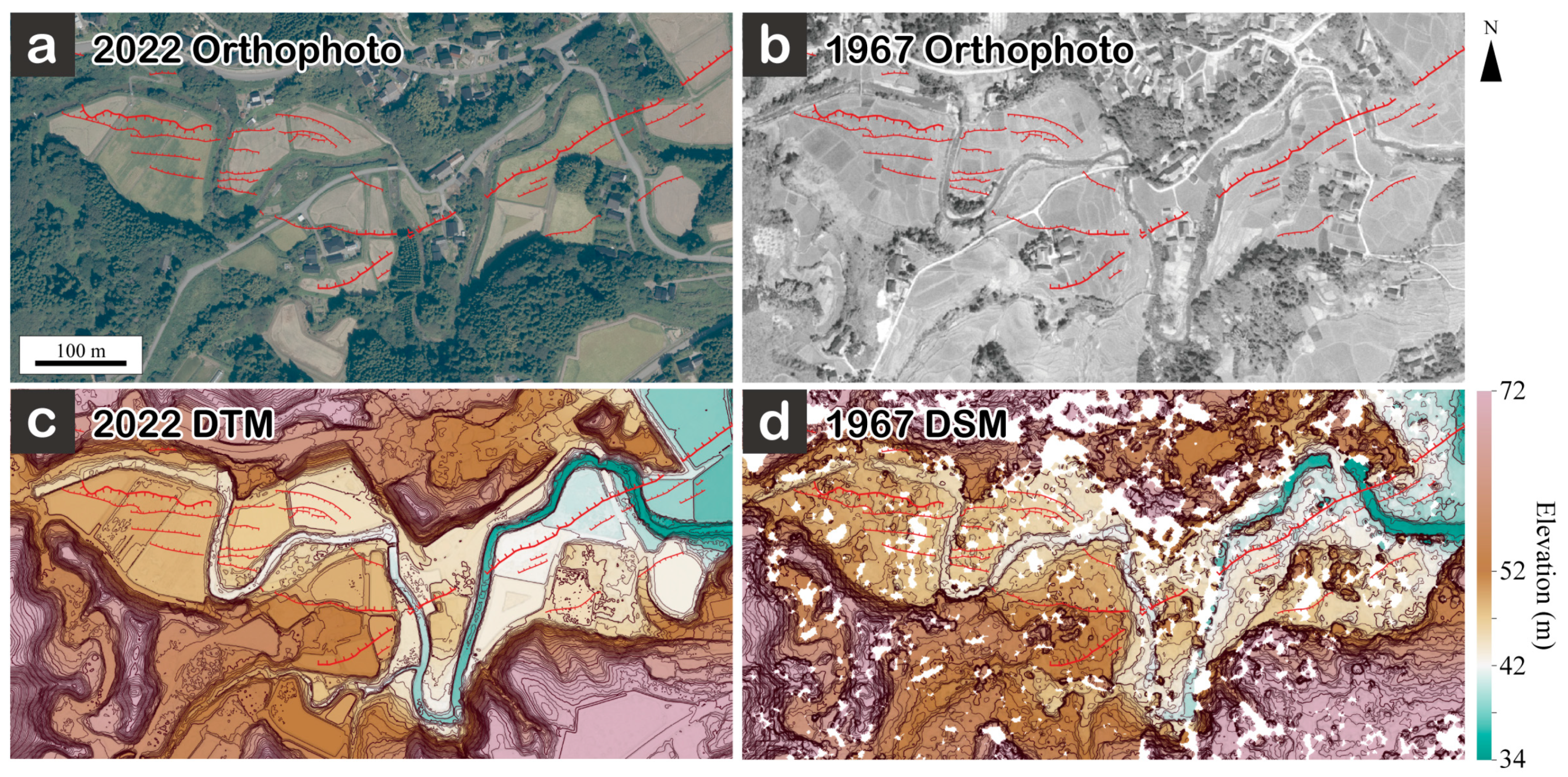
3.3. Pre-Earthquake Historical DSM (1967DSM)

The DSM was generated through SfM–MVS analysis using 12 MCB676X aerial photographs of the study area captured by the GSI on 30 April and 5 May 1967. These photographs had ground pixel dimensions of approximately 40 cm and were in JPEG format, having been scanned from an aerial photo film at 1270 dpi.

3.3.1. SfM Point-Cloud and DSM Generation

The tie points, depth maps, and high-density clouds were generated using the same settings as those used for the 2024DSM (Section 3.2). Interpolation was set to “Disabled” to generate a DSM with a resolution of 85 cm/pix from the point cloud. This DSM was transformed by reprojection in QGIS into a DSM with a resolution of 1 m (Japan Plane Rectangular Coordinate System 7; EPSG: 6675) through mean-value resampling using ‘gdalwarp’. As a DSM, it displays surface heights, including vegetation height.

3.3.2. Ground Control Point (GCP) Assignment

A total of 10 GCPs were selected within the study area. In a process similar to that described for the 2024DSM (Section 3.2.2), the latitude, longitude, and height of the GCPs were determined using a photographic map from the “FY2022 Forest Information Improvement Project” conducted by Ishikawa Prefecture from August to October 2022, with a numerical topographic model (2022DTM) created from 3D point-cloud data. The total RMSE of the GCP was 0.35 m (0.299 pix), assuming an accuracy of 1.0 m.

3.3.3. Orthomosaic Generation

A DSM was generated from the point cloud with interpolation set to “Enabled (default)”. Subsequently, an orthomosaic (42.5 cm/pix) was generated using the DSM as the source.

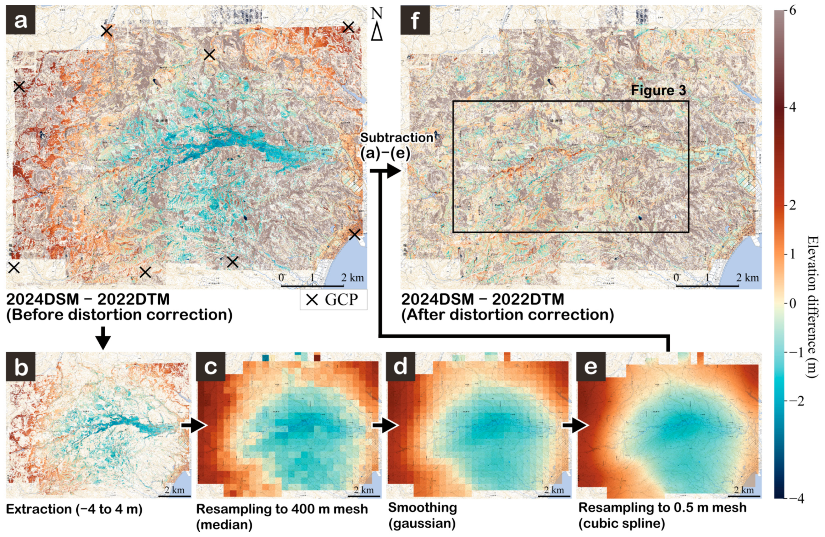
3.4. DEMs of Difference (DoDs)

To determine the extent of topographic change before and after the earthquake, DoDs were created using 2024DSM and 2022DTM, both with a resolution of 0.5 m. To examine the misfit between DEMs, raw DoDs were created (Figure 2a). Figure 2a reveals the presence of a concave distortion [20], a type of systematic doming effect [21,22] caused by 2024DSM. This distortion causes the DoD to exhibit dome-shaped artifacts with negative values at the center of the study area and positive values at the periphery. These bowl-shaped distortions are modeled based on resampling and smoothing technique and are then subtracted from the raw DoD to remove the distortions. The details are as follows. First, we examined several cells of the raw DoD on roads, excluding areas with vegetation, around the central and peripheral areas. As a result, the maximum absolute value of the raw DoD was observed to be about 4 m. Therefore, to eliminate as much as possible the effect of changes in ground elevation due to vegetation, we extracted only cells with raw DoD absolute values less than 4 m (Figure 2b). Next, to exclude localized effects and extract only dome-like distortions, the DoD was transformed to a resolution of 400 m by median resampling using gdalwarp in QGIS (Figure 2c). This resolution was obtained through trial and error to clearly visualize the distorted component of the dome shape. To remove errors due to surface deformation, smoothing was performed using a Gaussian filter in the GIS software SAGA (version 9.4.0) (Figure 2d), following which the resolution was transformed back to 0.5 m using a cubic spline in gdalwarp (Figure 2e) to obtain a corrected value. Subtracting this correction value from the original DEM eliminated the dome distortion (Figure 2f). The composite error (RMSE) of the DoD was 0.35 m, as estimated from the root sum square of the RMSEs of the pre-and post-earthquake DEM (2022DTM and 2024DSM) heights.

4. Results

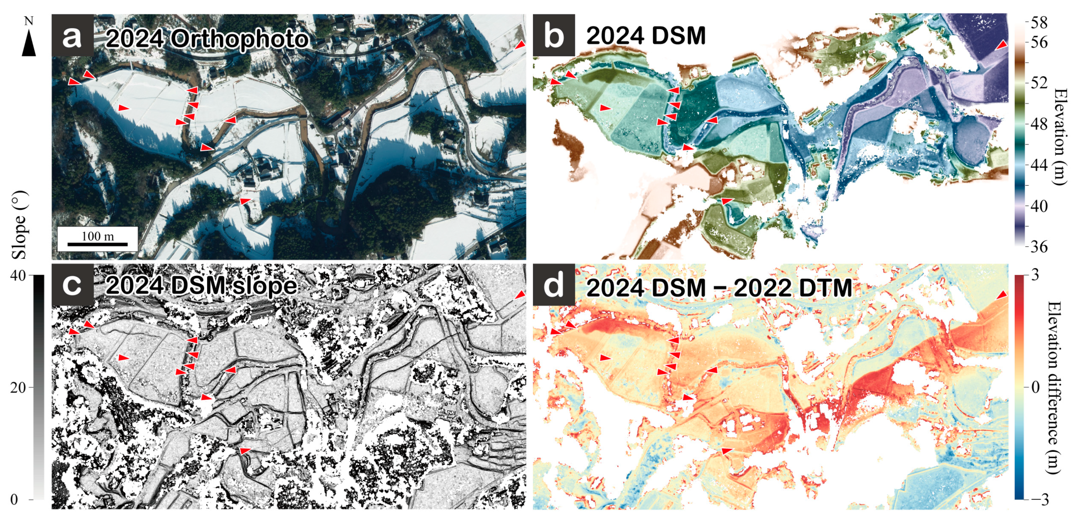
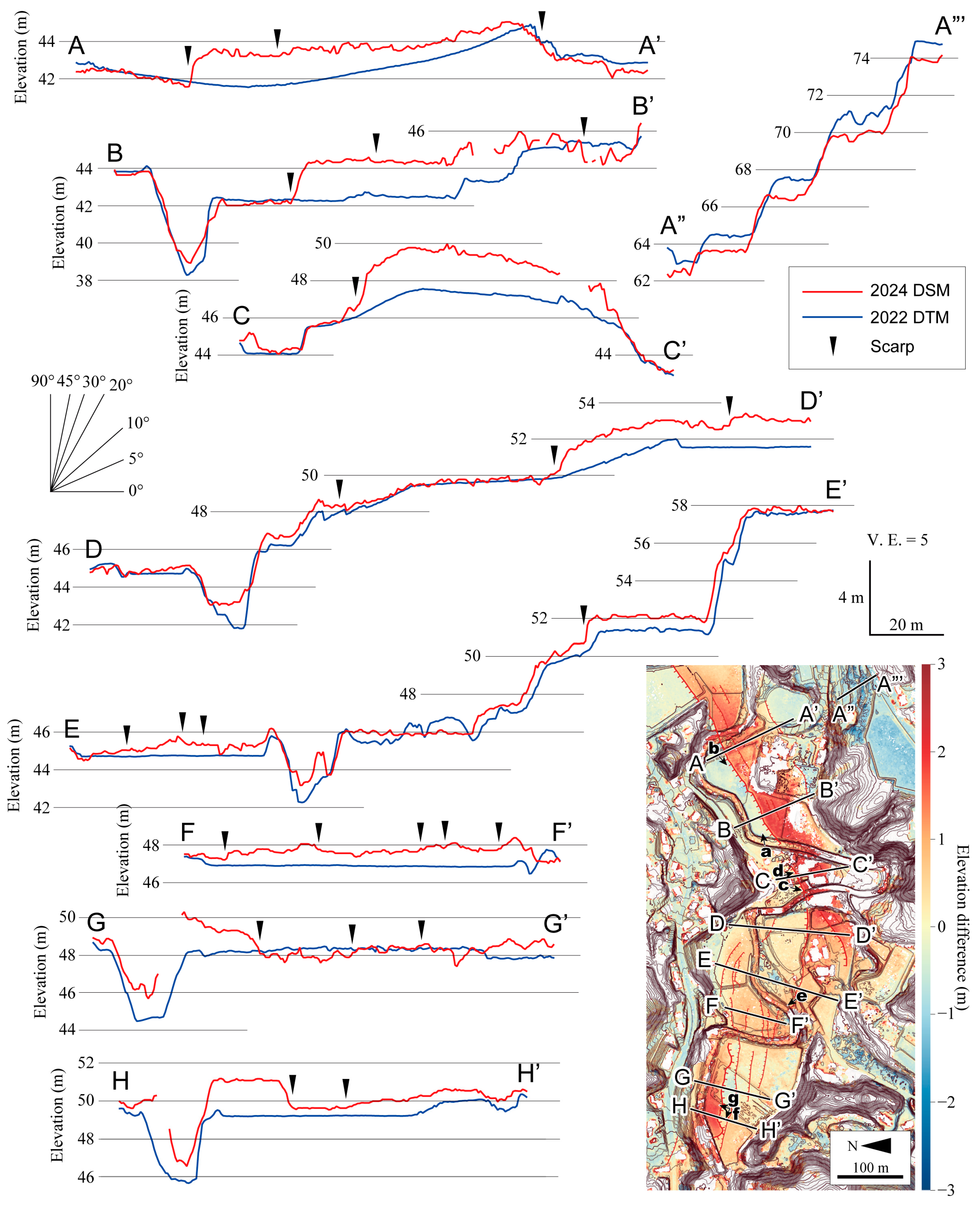
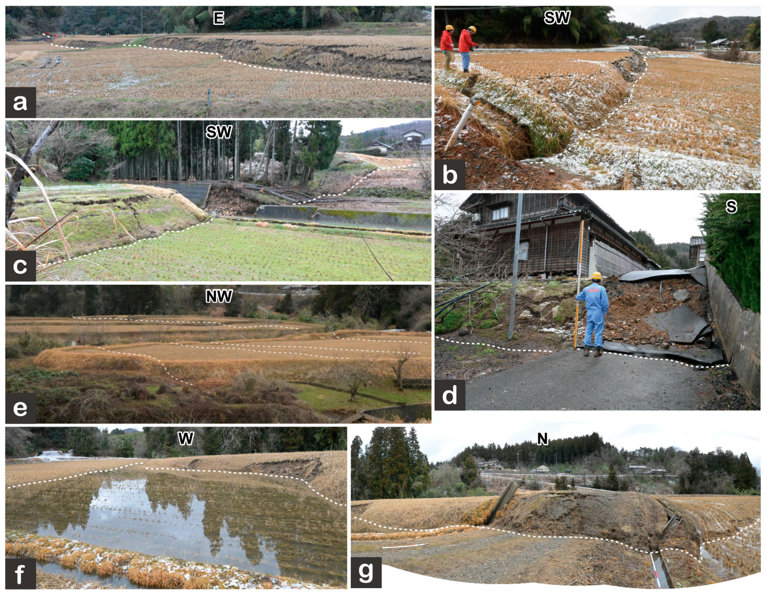
4.1. Regional Characteristics of Surface Deformation

Figure 3 shows the DoD in the area where surface deformation was observed. The surface deformation appeared intermittently along the valley floor of the Wakayama River, extending over a length of approximately 5 km (approximately 1 km in the eastern part and 4 km in the central and western parts). The DoD was primarily positive along the surface deformation, suggesting the presence of an uplift zone along the valley floor (blue dashed area in Figure 3). These surface deformations were distributed in close agreement with the location of the Okata anticline within the east–northeast-to-west–southwest synclinorium structure recognized by the 1:50,000 geologic map survey. The western edge of the surface deformation coincided with the western edge of the Okata anticline and Kumantani syncline.

The general trend of the relative horizontal displacement predominantly followed a southwest direction on the northern slopes (mountain slopes north of the Wakayama River) and a northwest direction on the southern slopes (mountain slopes south of the Wakayama River) relative to the surface deformation.

The extent of horizontal displacement was greater on the southern slope than on the northern slope. Specifically on the southern slope, horizontal displacements approximately exceeding 2 m were widely distributed from the central part (Figure 4a) to the western part (Figure 4b) of the surface deformation, covering approximately 4 km east–west and 2 km north–south, with the maximum displacement observed at 3.1 m. The southern limit of this range coincides with the main ridge of Mt. Horyuzan (elevation 468.5 m). In contrast, the northern slope exhibited a maximum displacement of 3.6 m locally, predominantly within the area identified as landslide topography (Figure 1d), which was attributed to the movement of a landslide mass spanning approximately 1 km in length and 0.5 km in width.

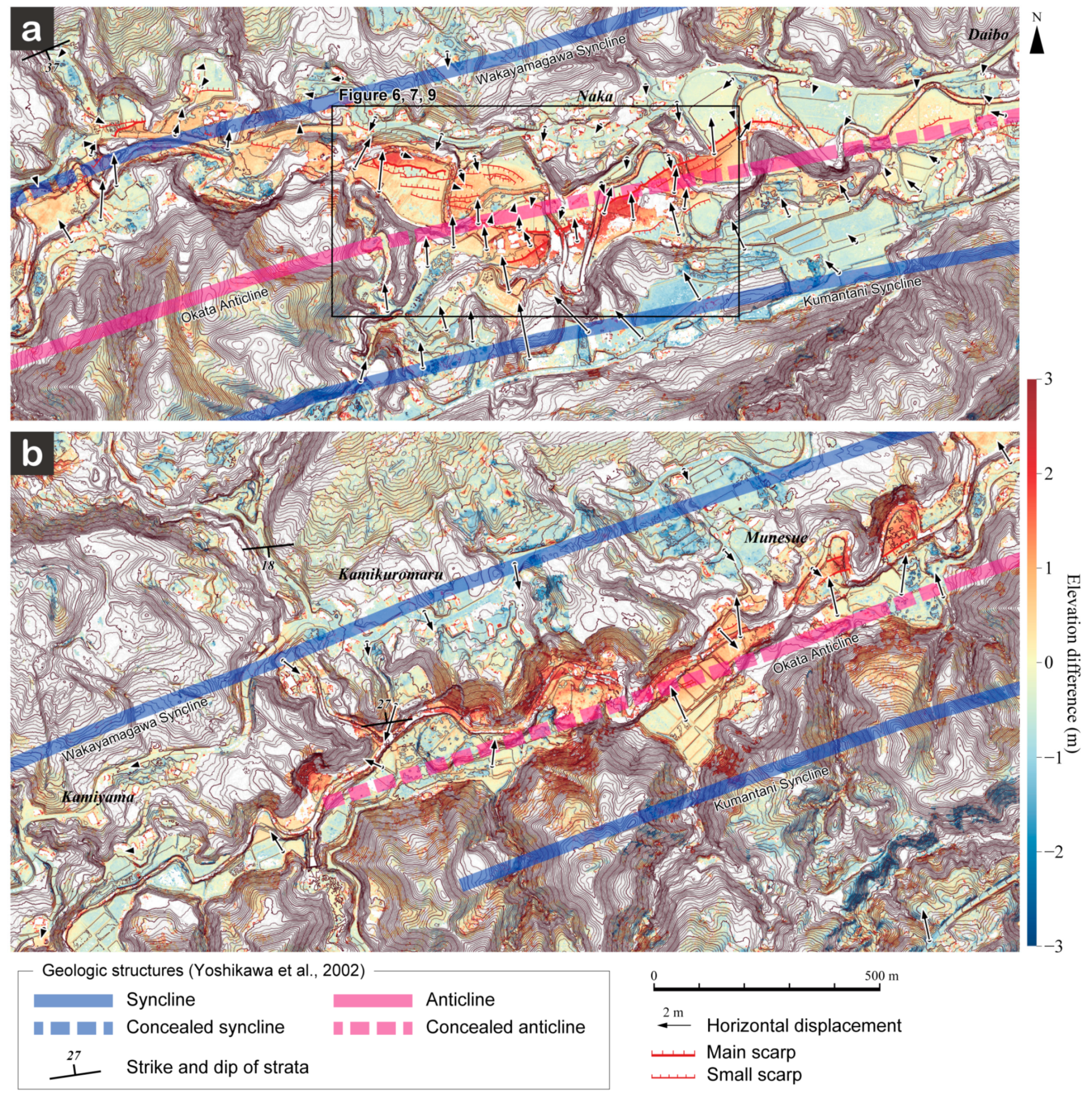
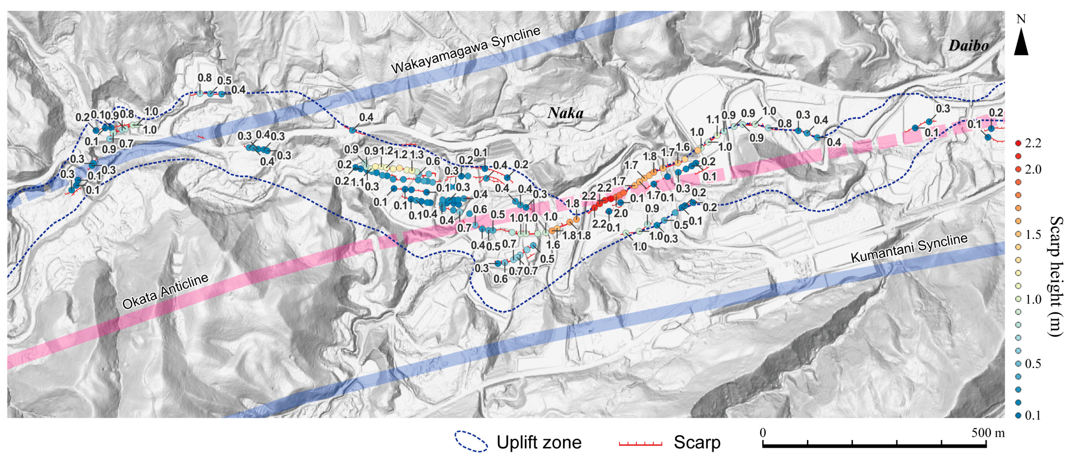
4.2. Characteristics of the Central Area

An enlarged view of the central-western surface-deformation area (approximately 4 km long) is depicted in Figure 4a. This area exhibited the most prominent surface deformation among those surveyed. Several scarps were aligned parallel to the floor of the Wakayama River valley, with their orientation almost consistent with the general direction of the valley axis. In the eastern half, scarps were oriented east–northeast to west–southwest, while in the western half, they were oriented east–southeast to west–northwest. The width of the uplift zone measured approximately 80–200 m in the eastern half, 200 m in the western half, and 400 m at their interface. In the northern and southern uplift zones, the DoD was predominantly negative, suggesting the occurrence of a subsidence zone at the mountain base along the margin of the valley floor.

4.2.1. Eastern Half of the Central Area (Eastern Part of the Naka Area of Wakayama Town)

The most major scarp in the eastern half (eastern part of the Naka area of Wakayama Town) exhibited a maximum vertical displacement of approximately 2.2 m, forming south-side-up steps (Figure 5). This scarp was the northernmost of the parallel scarps in the area (Figure 4a and Figure 6). The cross sections A-A′, B-B′, and C-C′ in Figure 7 illustrate the pre- and post-earthquake DEM profiles (2024DSM and 2022DTM) of the surface deformation in the eastern half. Although the 2024DSM contains more errors, including fine noise and missing points, compared to the 2022DTM, it indicates a larger overall vertical displacement (uplift) near the northernmost scarp. Both cross-sections reveal that the interior of the uplifted zone maintained a relatively smooth surface, preserving the original topography. In the C-C′ cross-section, an uplift reaching approximately 2 m was observed only when the original topography was convex. The relative horizontal displacement showed a compressive movement from both the north and south toward the uplifted zone, with a maximum horizontal displacement of 1.1 m in the north and 2.0 m in the south (Figure 4a). The orientation boundaries of this horizontal displacement coincided with the main scarp described above. Post-earthquake field photographs of this area are shown in Figure 8a–d. The slope of the scarp was also covered by the original terrain, which consisted of heaped-up arable-land surface and asphalt pavement from the road, indicating that the ground on the south side of the scarp rose toward the ground on the north side of the scarp.

4.2.2. Western Half of the Central Area (Western Part of the Naka Area of Wakayama Town)

The major scarp in the western half (western part of the Naka area of Wakayama Town) is located closer to the north of the parallel scarp, exhibiting a north-side-up of up to approximately 1.4 m (Figure 5). Located centrally within the uplift zone, this major scarp shows intermittent decreases in uplift towards the north and south, with the central part displaying a graben-like depressed deformation (Figure 4a). In Figure 7, cross-sections E-E′, F-F′, G-G′, and H-H′ depict DEM profiles of this western half of the surface deformation before and after the earthquake (2024DSM, 2022DTM). The overall trend indicates minor displacement along each scarp, with the northern scarps showing north-side-up and the southern scarps south-side-up, viewed from the center of the uplift zone.

Relative horizontal displacement compressed the ground from the north and south toward the uplift zone, with maximum displacements of 1.0 m in the north and 2.2 m in the south (Figure 4a). The azimuthal boundary of this horizontal displacement coincided with the major scarp described above. Unlike the main scarp in the eastern half, this scarp exhibited a curved planform and locally showed a right-lateral displacement of approximately 1.0 m (Figure 8g). Moreover, this localized right-lateral offset was evident as an eastward displacement in the horizontal displacement measurements in the uplift zone north of the main scarp (Figure 4a).

4.2.3. Middle Part of the Central Section (Central Part of the Naka Area of Wakayama Town)

In the middle part, which is located between the eastern and western halves, the primary scarp of the eastern half splits into two segments. The northern segment aligns with the east–southeast to west–northwest strike observed in the western half, while the southern segment maintains an orientation almost identical to that of the eastern half. Both segments disappear approximately 200 m to the west (Figure 4a).

The relative horizontal displacement showed a northward shift north of the two scarps (Figure 4a). The orientation boundary of the horizontal displacement was located at the center of the uplift zone, near the meandering axis of the Wakayama River, and no major scarps were observed at this boundary point. The extent of horizontal displacement was smaller in the northern direction than at the two main scarps, with the boundary point showing negligible horizontal displacement. The horizontal displacements reached maxima of 0.9 m in the north and 3.1 m in the south (Figure 4a).

In Figure 7, cross-section D-D′ shows the pre- and post-earthquake (2024DSM and 2022DTM) topographic profiles of this intermediate surface deformation. In this area, northern scarp with north-side-up and southern scarp with south-side-up are located, viewed from the center of the uplift zone. In addition, the two main southern scarps created a significant step ranging from approximately 0.7 to 1.0 m (Figure 5).

Of these the two main scarps, the northern scarp follows the cliff topography from 1967 to the present (Figure 9c,d). The other scarp, however, does not coincide with the 1967 cliff and land-use boundaries (Figure 9).

4.3. Characteristics of the Western Part (the Munesue and Kamikuromaru Areas of Wakayama Town)

An enlarged view of the western portion of the central–western surface deformation (approximately 4 km in length) is shown in Figure 4b. Several scarps were observed on parts of the Wakayama River valley floor; however, they were indistinct and intermittent. The strike of the scarps almost coincided with the general direction of the valley axis of the Wakayama River valley floor, exhibiting an east–southeast to west–northwest orientation. The width of the uplift zone was approximately 200–300 m.

Relative horizontal displacement was observed to have compressed the ground from the north and south toward the uplift zone, with a maximum horizontal displacement of 2.2 m (Figure 4b). The orientation boundary of this horizontal displacement roughly coincided with the location of the Wakayama River.

The western edge of the uplift zone roughly coincided with the western edge of the Okata anticline. In the north and south of the uplift zone, the DoD was negative and parallel to the uplift zone, suggesting the presence of a subsidence zone at the mountain’s base.

4.4. Characteristics of Surface Deformation in the Eastern Area (the Nobutake Area of Wakayama Town)

An enlarged view of the eastern surface deformation (approximately 1 km long) is shown in Figure 10 and Figure 11a. Three parallel scarps were observed, indicating an east–southeast to west–northwest strike. The width of the uplifted zone was approximately 150–200 m, and its northern and southern edges roughly coincided with the locations of the scarps.

In Figure 11b, cross-section K-K′ shows the pre- and post-earthquake (2024DSM and 2022DTM) DEM profiles of the eastern surface deformation. The northern scarp did not show a sharp step; instead, it showed a gradual south-side-up, while the central and southern scarps showed a north-side-up. The vertical displacement of each scarp was small, ranging from 0.1 to 0.4 m. Since 1967, the eastern part of the uplifted zone has served as residential land or upland fields, making these areas different in terms of land use from the surrounding rice paddies (Figure 12a,b). This zone shows a wide river-terrace surface; however, only the distribution area of the uplifted zone in the 1967DSM is approximately 1 m higher in elevation than the northern side of the terrace surface (Figure 12d). At the eastern end of the uplift zone are higher terraces with cliffs of the same strike as the scarps (Figure 12c).

The relative horizontal displacements were smaller (up to 1.0 m) than those near the central-western surface deformation (Figure 11a). The orientation of the horizontal displacement was southwest from the northern part of the uplift zone to the southern end of the uplift zone and northwest in the southern part of the uplift zone, indicating that the horizontal displacement had compressed the ground at the southern end of the uplift zone.

5. Discussion

5.1. Causes of Surface Deformation

Although the detailed causes of surface deformation in this area require further investigation using trenching and seismic reflection surveys, some possible causes can be inferred based on the topographic features observed in this study.

Surface deformation in this area was confined to the vicinity of the Okata anticline. These surface deformations were likely caused by fault activity because most of the active faults around the Noto Peninsula formed along anticline structures during the late Miocene [5].

The main fault of the Noto Peninsula earthquake (Mw7.5) has been estimated to be located on the seafloor, approximately 2 km north of the northern shore of the Noto Peninsula, and it is characterized as a south-up reverse fault [2]. If the surface deformation in the study area is a backthrust (primarily distributed ruptures) [23] connected deep in the subsurface to an epicenter fault in the ocean, it would be expected to be a north-side-up reverse fault. However, the major scarp in this region is characterized by a south-side-up displacement, indicating a reverse trend. Therefore, it is not directly related to the Noto Peninsula earthquake (Mw7.5) source fault but may be a passively formed triggered rupture.

Surface deformation was observed exclusively at locations congruent with the distribution of the synclinorium structures. The uplift and subsidence areas inferred from the DoD were directly located above the anticlines and synclines of the synclinorium structure, respectively. Horizontal displacements directly above the two synclines of the synclinorium structure were oriented in opposite directions, converging towards the dorsal oblique where the uplifted area occurred. Hence, it can be interpreted as deformation within an active fold, where the fold structure develops under horizontal compression. In a nearby area approximately 130 km to the east, the earthquake-triggered activity of a subsurface fault plane leading to active old growth has been reported following the 2007 Niigata-ken Chuetsu-oki earthquake (M6.8) [24].

Flexural slip and bending moment are typical fault mechanisms associated with folding [25]. The graben-like topography observed in the uplifted area in the western half of the central section (western part of the Naka area of Wakayama Town), as seen in cross-sections E-E′, F-F′, G-G′, and H-H′ in Figure 7, may result from normal faulting associated with the bending moment [26,27] caused by layer-parallel stretching during anticline growth. Conversely, the large vertical-displacement scarp in the eastern half of the central section (eastern part of the Naka area of Wakayama Town) may indicate reverse faulting due to bending moments [26] caused by layer-parallel shortening within the Kumantani syncline. Alternatively, the Okata anticline may represent a bending-moment deformation developed between the two synclinorium structures at the hinge line. In contrast, the surface deformation observed in the eastern half of the central section (eastern part of the Naka area of Wakayama Town) could potentially be a reverse fault resulting from the movement of an existing bending-moment fault. In certain areas within the central part (central part of the Naka area of Wakayama Town) and eastern part (Nobutake area of Wakayama Town), scarps were observed to align harmonically with existing terrace cliffs (Figure 9 and Figure 12) or the existing convex topography was uplifted harmonically (C-C′ in Figure 7). Some of the scarps identified in this study may have also undergone cumulative topographical modification due to past earthquakes.

Numerous landslide landforms exist on mountain slopes surrounding surface deformation in the central and western areas. As the horizontal displacement of mountain slopes is in the same direction as the slope dip, there is a likelihood of finding terminal cliffs associated with landslide movement. However, the area of large horizontal displacement on the southern slope was approximately ten times larger than the area in which individual landslide landforms were distributed (Figure 1d), and no landslide landforms of this size were observed. Furthermore, rather than typical landslide-induced terminal cliffs, the area around the landslide exhibited a sharp and straight scarp, with the surrounding area maintaining a smooth original topographic surface without any disturbed landforms visible. Additionally, although landform boundaries, such as a sliding cliffs at the mountain top and lateral cliffs and cracks at the sides of a landslide, could potentially have formed, these landforms were not identified through aerial photo-reading or DoD analysis. Future topographic analysis using the LiDAR DTM will clarify the presence or absence of these landforms, and their relationship with landslides should be carefully examined. Notably, the eastern surface deformation (the Nobutake area of Wakayama Town) is not adjacent to a mountain slope, and landslide landforms were not observed in the vicinity. Therefore, even if the central-to-western surface deformation is attributed to landslides, a different factor may have caused the eastern surface deformation.

5.2. Advantages of Aerial Photographs and SfM–MVS in Preliminary Surveys

Aerial photographs captured by manned aircrafts to assess damage immediately after an earthquake offer several advantages over other remote-sensing techniques [12]. While unmanned aerial vehicle (UAV) surveys and ground-based laser measurements excel in capturing detailed topographic features [28], they may overlook broad-scale or less distinct deformations. In addition, aerial laser surveying can accurately measure vegetated areas but is expensive and time-consuming. Therefore, acquisition of LiDAR data in a quick and cost-effective manner is dependent on identifying areas of surface deformation in advance. Satellite imagery often lacks the resolution necessary for detecting small displacements, and interferometric synthetic aperture radar (InSAR) can lose data with substantial crustal deformation [29], rendering it unable to precisely assess surface deformation along the Wakayama River. The GSI promptly captures aerial photographs in Japan within a few days of an earthquake. The SfM–MVS techniques using these aerial photographs are effective in quickly identifying areas of surface deformation measuring several tens of centimeters or more after earthquake disasters despite facing certain challenges, as described below.

5.3. Location Accuracy of GCPs Immediately after the Earthquake

The GCP locations and heights used in this study were determined based on orthoimages and DTMs created before the earthquake. Owing to extensive crustal deformation caused by the earthquake in this region, accurate measurement of position and height values post-earthquake is essential. However, obtaining on-site global navigation satellite system (GNSS) observations immediately after an earthquake is challenging because of road damage caused by landslides and other factors. In contrast, to visualize only local topographic changes, such as surface deformation in this area, it is crucial to eliminate the effects of wide-area crustal deformation. Therefore, obtaining GCPs aligned with pre-earthquake positions is an important step needed to improve relative positional accuracy.

The GCP heights were adjusted to post-earthquake values using the pixel offset results from the SAR analysis. This adjustment likely contributes to the smaller Z error compared to the XY error in the context of GCP accuracy. However, the impact of a large or small Z-component error on the systematic bowl-shaped error has yet to be determined and will be investigated in future studies.

5.4. Removal of Systematic Errors

In SfM–MVS analysis using aerial photographs containing post-earthquake surface deformation, obtaining GCPs around the deformation area (near the center of the photographic model) is challenging. Consequently, the 3D point clouds and DSM obtained through SfM–MVS can exhibit bowl-like distortions [20,30]. While incorporating oblique photographs [21] and increasing the number of GCPs [22] are effective strategies for mitigating this systematic error. However, the camera used for capturing these aerial photographs in this study produced only vertical photographs. In addition, the surface deformation located at the center of the model. Therefore, the addition of GCPs was deemed inappropriate. In this study, systematic errors were corrected by rasterizing the DoD; however, the accuracy could be further improved by calculating and correcting the degree of DSM deformation, such as the curvature and slope [30]. After correcting for systematic errors, the absolute accuracy of the vertical displacement obtained from DoD requires further investigation.

In this study, an extraction method for relative topographic change is considered effective if the approximate location of the surface deformation is known in advance and local, linear topographic changes are to be visualized. However, for surface deformations with dome- or bowl-shaped topographic changes over a wide area (e.g., subsidence of plains and volcanic uplift/subsidence), distinguishing them from systematic errors using SfM–MVS is difficult, making this method potentially unsuitable.

5.5. Cautions for Deciphering the DoD

Based on the composite error results of the DoD, any displacement greater than ~0.35 m can be classed as extremely significant surface deformation. Accurately deciphering topographic or surface elevation changes was difficult at times because the DoDs generated by this method are DTMs for pre-earthquake periods and DSMs for post-earthquake periods. Ideally, the DTM and DSM from each period should be presented, and the DoD should be generated from DTM to DTM or DSM to DSM. In this case study, LiDAR DTMs could not be obtained by the aircraft immediately after the earthquake because of the seasonal snow and the extensive size of the area affected by the earthquake. In addition, because the pre-earthquake DSM (2022DSM) was measured during the summer season, generating a DoD [9] between the 2024DSM and 2022DSM resulted in a difference between the crown and ground heights in areas with deciduous trees, making it difficult to interpret the DoD for this study.

SfM–MVS using aerial photographs captured immediately after an earthquake can produce DTMs with some difficulty but can achieve heights equivalent to DTMs in areas where the ground is visible, such as areas without vegetation or buildings. In addition, as aerial photographs often provide data earlier than LiDAR DTMs, they can be used for preliminary surveys immediately after an earthquake. However, because the 2024DSM data correspond to the snowy season, some ground surfaces in well-sunlit areas were visible in the aerial photographs; however, the data included areas covered by snow depths of approximately 5–30 cm. Consequently, some of the 30-cm changes in DoD reflect surface-height differences due to snow rather than to actual topographic changes. In addition, surface deformation in evergreen forests is difficult to ascertain and requires further scrutiny through LiDAR DTM measurements.

Aerial SfMs have been reported to show almost the same values of ground pixel dimensions and absolute positional accuracy [31]. Similarly, for the 2024DSM in this study, the position and height accuracy (RMSE) and ground pixel dimensions were close to ~40 cm. This suggests that capturing surface deformations of less than 10 cm would be difficult. However, aerial SfM detected a scarp with a step difference of approximately 10 cm, indicating that it has the relative accuracy needed to detect surface deformations with smaller displacements.

6. Conclusions

Aerial SfM–MVS, using photographs taken from a manned aircraft immediately after the earthquake, can be used to accurately map the surface deformation caused by the earthquake. The accuracy of this study needs to be verified further using post-earthquake wide-area LiDAR measurement data. Nevertheless, this method is effective for early and simple detection of local linear and strip-like surface deformations in earthquake disasters involving wide areas and large fluctuations. For fields, grasslands, rice paddies, and bare land, excluding forested areas, data with absolute accuracy similar to the DTM of aircraft LiDAR can be obtained.

The surface deformation along the Wakayama River is extremely short, localized, and distant compared to the submarine active fault that caused the Noto Peninsula earthquake. Therefore, this surface deformation is considered to have been caused secondarily by the earthquake rather than by a branch fault. In addition, the surface deformation with uplift zones occurred only in areas of synclinorium structure where synclinorium and anticlines are extremely close. Therefore, surface deformation is largely related to faulting and the development of folds. Some surface deformations that are in harmony with the cliff topography that existed before the artificial alterations of the 1970s have also occurred. The cliff topography may have been created by cumulative displacement of the Okata anticline.

Landslides on the surrounding slopes (especially on the southern slope) were displaced in a similar direction and to a similar degree over a wide area along the Wakayama River. This suggests that the landslides did not occur locally and independently but may have been active in conjunction with the geomorphic development of the uplift zone along the Wakayama River.

References

- Japan Meteorological Agency. JMA CMT Solution. 2024. Available online: https://www.data.jma.go.jp/eqev/data/mech/cmt/fig/cmt20240101161022.html (accessed on 30 July 2024). (In Japanese)
- Headquarters for Earthquake Research Promotion. Evaluation of the 2024 Noto Peninsula Earthquake. 9 February 2024. Available online: https://www.static.jishin.go.jp/resource/monthly/2024/20240101_noto_3.pdf (accessed on 30 July 2024). (In Japanese)
- Geospatial Information Authority of Japan. Crustal Deformation Associated with the 2024 Noto Peninsula Earthquake Based on Analysis of “Daichi-2” Observation Data. 19 January 2024. Available online: https://www.gsi.go.jp/uchusokuchi/20240101noto_insar.html (accessed on 30 July 2024). (In Japanese)
- Inoue, T.; Okamura, Y. Explanatory Notes of 1:200,000 Marine Geological Map Around the Northern Part of Noto Peninsula. Seamless Geoinformation of Coastal Zone “Northern Coastal Zone of Noto Peninsula”. 26 February 2010. Available online: https://www.gsj.jp/data/coastal-geology/GSJ_DGM_S1_2010_01_b.pdf (accessed on 30 July 2024).
- Okamura, Y. Distribution of Active Faults in Japan Sea and Future Issues. Zisin 2019, 71, 185–199, (In Japanese with English Abstract). [Google Scholar] [CrossRef]
- Japan Coast Guard. Survey of Seafloor Topography Related to the 2024 Noto Peninsula Earthquake. 2024. Available online: https://www1.kaiho.mlit.go.jp/jishin/meeting/398chosa.pdf (accessed on 30 July 2024). (In Japanese)
- Okamura, Y.; Ogami, T.; Inoue, T.; Sato, T.; Arimoto, J. Report on the Urgent Investigation of the 2024 Noto Peninsula Earthquake (Displacement of Submarine Active Faults Associated with the 2024 Noto Peninsula Earthquake). 2024. Available online: https://www.gsj.jp/hazards/earthquake/noto2024/noto2024-10.html (accessed on 30 July 2024). (In Japanese).
- Geological Survey of Japan, AIST. Seamless Digital Geological Map of Japan V2 1:200,000, Original Edition. 2023. Available online: https://gbank.gsj.jp/seamless/ (accessed on 14 May 2024).
- Yoshikawa, T.; Kano, K.; Yanagisawa, Y.; Komazawa, M.; Joshima, M.; Kikawa, E. Geology of the Suzumisaki, Noto-iida and Hōryūzan District; Quadrangle Series; 1:50,000; Geological Survey of Japan, AIST: Tsukuba, Japan, 2002; p. 76, (In Japanese with English abstract 4p). [Google Scholar]
- Ishiguro, S.; Kumahara, Y.; Goto, H.; Nakata, T.; Matsuta, N.; Sugito, N.; Hirouchi, D.; Watanabe, M.; Sawa, H.; Suzuki, Y. Evaluation of high-resolution digital surface models of surface rupture associated with the 2014 Kamishiro Fault Earthquake, Central Japan, using unmanned aerial vehicle photography and SfM-MVS analysis. J. Remote Sens. Soc. Jpn. 2016, 36, 107–116, (In Japanese with English Abstract). [Google Scholar] [CrossRef]
- Yamazaki, F.; Kubo, K.; Tanabe, R.; Liu, W. Damage assessment and 3d modeling by UAV flights after the 2016 Kumamoto, Japan earthquake. In Proceedings of the 2017 IEEE International Geoscience and Remote Sensing Symposium (IGARSS), Fort Worth, TX, USA, 26 July 2017; pp. 3182–3185. [Google Scholar]
- Andreuttiova, L.; Hollingsworth, J.; Vermeesch, P.; Mitchell, T.M.; Bergman, E. Revisiting the 1959 Hebgen Lake earthquake using optical image correlation; new constraints on near-field 3D ground displacement. Geophys. Res. Lett. 2022, 49, e2022GL098666. [Google Scholar] [CrossRef]
- Delano, J.E.; Howell, A.; Stahl, T.A.; Clark, K. 3D Coseismic surface displacements from historical aerial photographs of the 1987 Edgecumbe Earthquake, New Zealand. J. Geophys. Res. Solid Earth 2022, 127, e2022JB024059. [Google Scholar] [CrossRef]
- Yoshida, K. Linear Surface Deformation with Vertical Displacement Appeared in Wakayama Town, Suzu City, Ishikawa Prefecture (Preliminary Report). 2024. Available online: https://www.gsi.go.jp/common/000254854.pdf (accessed on 30 July 2024). (In Japanese)
- Shirahama, Y.; Ishiyama, T.; Tateishi, R.; Yasue, K. Surface Ruptures Appeared along the Wakayama-Gawa River Associated with 2024 Noto Peninsula Earthquake (Preliminary Report). 2024. Available online: https://www.eri.u-tokyo.ac.jp/news/20465/ (accessed on 30 July 2024). (In Japanese).
- Yoshimi, M.; Maruyama, T. Report on the Urgent Investigation of the 2024 Noto Peninsula Earthquake (Field Survey of Land Surface Deformation Appearing on Land). 2024. Available online: https://www.gsj.jp/hazards/earthquake/noto2024/noto2024-09.html (accessed on 30 July 2024). (In Japanese).
- Ishida, S. The Cenozoic Strata of Noto, Japan. Mem. Coll. Sci. Univ. Kyoto Ser. B 1959, 26, 83–101. [Google Scholar]
- Ota, Y.; Matsuda, T.; Hirakawa, K. Active faults in Noto Peninsula, Central Japan. Quat. Res. (Dai-yonki-Kenkyu) 1976, 15, 109–128, (In Japanese with English Abstract). [Google Scholar] [CrossRef]
- Over, J.R.; Ritchie, A.C.; Kranenburg, C.J.; Brown, J.A.; Buscombe, D.; Noble, T.; Sherwood, C.R.; Warrick, J.A.; Wernette, P.A. Processing Coastal Imagery with Agisoft Metashape Professional Edition, Version 1.6-Structure from Motion Workflow Documentation; U.S. Geological Survey: Woods Hole, MA, USA, 2021. [CrossRef]
- Nakata, Y.; Iwasaki, K.; Shimada, S.; Torita, H. Understanding microtopography changes in agricultural landscapes through precision assessments of digital surface models by the UAV-RTK-PPK method without ground control points. Smart Agric. Technol. 2023, 5, 100269. [Google Scholar] [CrossRef]
- James, M.R.; Robson, S. Mitigating systematic error in topographic models derived from UAV and ground-based image networks. Earth Surf. Process. Landf. 2014, 39, 1413–1420. [Google Scholar] [CrossRef]
- Eltner, A.; Baumgart, P.; Maas, H.-G.; Faust, D. Multi-temporal UAV data for automatic measurement of rill and interrill erosion on loess soil. Earth Surf. Process. Landf. 2015, 40, 741–755. [Google Scholar] [CrossRef]
- Nurminen, F.; Baize, S.; Boncio, P.; Blumetti, A.M.; Cinti, F.R.; Civico, R.; Guerrieri, L. SURE 2.0—New release of the worldwide database of surface ruptures for fault displacement hazard analyses. Sci. Data 2022, 9, 729. [Google Scholar] [CrossRef] [PubMed]
- Nishimura, T.; Tobita, M.; Yarai, H.; Amagai, T.; Fujiwara, M.; Une, H.; Koarai, M. Episodic growth of fault-related fold in northern Japan observed by SAR interferometry. Geophys. Res. Lett. 2008, 35, L13301. [Google Scholar] [CrossRef]
- Yeats, R.S. Active Faults Related to Folding, in Active Tectonics; The National Academies Press: Washington, DC, USA, 1986; pp. 63–79. [Google Scholar]
- Li, T.; Chen, J.; Jobe, J.A.T.; Burbank, D.W.; Cheng, X.; Xu, J.; Li, Z.; Zheng, W.; Zhang, P. Active bending-moment faulting: Geomorphic expression, controlling conditions, accommodation of fold deformation. Tectonics 2018, 37, 2278–2306. [Google Scholar] [CrossRef]
- Livio, F.; Kettermann, M.; Reicherter, K.; Urai, J.L. Growth of bending-moment faults due to progressive folding: Insights from sandbox models and paleoseismological implications. Geomorphology 2019, 326, 152–166. [Google Scholar] [CrossRef]
- Liu-Zeng, J.; Yao, W.; Liu, X.; Shao, Y.; Wang, W.; Han, L.; Wang, Y.; Zeng, X.; Li, J.; Wang, Z.; et al. High-resolution structure-from-motion models covering 160 km-long surface ruptures of the 2021 MW 7.4 Madoi earthquake in northern Qinghai-Tibetan Plateau. Earthq. Res. Adv. 2022, 2, 100140. [Google Scholar] [CrossRef]
- Elliott, J.R.; Walters, R.J.; Wright, T.J. The role of space-based observation in understanding and responding to active tectonics and earthquakes. Nat. Commun. 2016, 7, 13844. [Google Scholar] [CrossRef] [PubMed]
- Mueller, M.M.; Dietenberger, S.; Nestler, M.; Hese, S.; Ziemer, J.; Bachmann, F.; Leiber, J.; Dubois, C.; Thiel, C. Novel UAV flight designs for accuracy optimization of structure from motion data products. Remote Sens. 2023, 15, 4308. [Google Scholar] [CrossRef]
- Ishiguro, S.; Yamano, H.; Oguma, H. Evaluation of DSMs generated from multi-temporal aerial photographs using emerging structure from motion–multi-view stereo technology. Geomorphology 2016, 268, 64–71. [Google Scholar] [CrossRef]