SimNFND: A Forward-Looking Sonar Denoising Model Trained on Simulated Noise-Free and Noisy Data

Abstract

Given the propagation characteristics of sound waves and the complexity of the underwater environment, denoising forward-looking sonar image data presents a formidable challenge. Existing studies often add noise to sonar images and then explore methods for its removal. This approach neglects the inherent complex noise in sonar images, resulting in inaccurate evaluations of traditional denoising methods and poor learning of noise characteristics by deep learning models. To address the lack of high-quality data for FLS denoising model training, we propose a simulation algorithm for forward-looking sonar data based on RGBD data. By utilizing rendering techniques and noise simulation algorithms, high-quality noise-free and noisy sonar data can be rapidly generated from existing RGBD data. Based on these data, we optimize the loss function and training process of the FLS denoising model, achieving significant improvements in noise removal and feature preservation compared to other methods. Finally, this paper performs both qualitative and quantitative analyses of the algorithm’s performance using real and simulated sonar data. Compared to the latest FLS denoising models based on traditional methods and deep learning techniques, our method demonstrates significant advantages in denoising capability. All inference results for the Marine Debris Dataset (MDD) have been made open source, facilitating subsequent research and comparison.

1. Introduction

Underwater environmental sensing technologies include acoustic, optical, and magnetic field detection. Acoustic technology is the main method for underwater sensing due to its long-distance propagation and extensive coverage [1,2,3]. A forward-looking imaging sonar is crucial for underwater detection and target identification, useful in fishing, navigation safety, military operations, maritime search and rescue, and ocean exploration [4]. Compared to optical systems, an imaging sonar provides long-distance information in low-visibility, high-light attenuation underwater conditions, making it effective in turbid waters. With technological advancements, the imaging sonar’s applications now include localization, object detection, mapping, and 3D reconstruction. These technologies have improved the efficiency of ocean infrastructure inspection and maintenance, advancing marine exploration and research.

Despite its advantages in underwater visibility, the forward-looking sonar faces several challenges and limitations in practice. Firstly, sonar images are usually presented in grayscale and affected by complex noise, limiting their ability to discern details and classify targets. Secondly, acquiring sonar datasets is complex, resulting in limited datasets that restrict the application and development of deep learning algorithms. Deep learning relies on high-quality data, which are fundamental to model performance. However, as shown in Figure 1, due to the lack of a noise-free benchmark for sonar images, most of current sonar denoising studies add artificial noise ${\mathbf{N}}_{artificial}$ to the actual collected sonar data $\mathbf{X}$ to obtain a noisy image $\mathbf{Y}$ as simulated noisy data, treating $\mathbf{X}$ as simulated noise-free data. These studies focus on how to remove the added artificial noise ${\mathbf{N}}_{artificial}$ and use the L1 loss between $\mathbf{Y}$ and $\mathbf{X}$ to evaluate denoising performance.

$$\mathbf{X}=\mathbf{T}+{\mathbf{N}}_{inherent},\mathbf{Y}=\mathbf{X}+{\mathbf{N}}_{artifical}.$$

(1)

However, $\mathbf{X}$ is actually composed of the true value $\mathbf{T}$ and inherent noise ${\mathbf{N}}_{inherent}$. Since there is currently no method to define a noise-free benchmark, i.e., the true value $\mathbf{T}$, most current sonar denoising studies can be regarded as approximations of transformations from the $\mathbf{Y}$ domain to the $\mathbf{X}$ domain, ignoring the inherent noise ${\mathbf{N}}_{inherent}$. Consequently, the denoising effects are rather limited and lead to significant flaws in the evaluation of denoising model performance in previous studies. Through the simulation method proposed in this paper, we define a completely noise-free true value $\mathbf{T}$ and construct the input $\mathbf{X}$, enabling the study to genuinely approach the transformation from the $\mathbf{X}$ domain to the $\mathbf{T}$ domain, which is the essence of the sonar denoising task.

Simulation technology offers an effective solution to this problem. By synthesizing noise-free benchmark data T and adding noise to construct noisy data X, it provides a foundation for the denoising research of sonar images. This paper proposes a forward-looking sonar data simulation technique using existing RGBD datasets. This technique aims to synthesize sonar datasets that are rich in environmental features and highly realistic and to use these datasets to train deep learning-based denoising models for forward-looking imaging sonars.

The primary contributions of this paper are summarized as follows:

• A forward-looking sonar sonar data simulation method based on RGBD data is proposed, eliminating the cumbersome manual construction of virtual scenes required by other simulation methods. This approach lays the groundwork for the rapid generation of large volumes of high-quality forward-looking sonar sonar simulation data.
• A simulated ground truth-based supervised training method for forward-looking sonar sonar denoising models is introduced. This method addresses the challenges in performance evaluation and incomplete denoising due to the absence of completely noise-free ground truth in previous research.
• A forward-looking sonar denoising model is trained, leveraging simulated noise-free and noise data and the new loss function. This guides the model to understand the imaging characteristics of the sonar, significantly enhancing the model’s denoising capability and detail retention for FLS data.

The rest of this paper is organized as follows: The Section 2 reviews the current state of research on forward-looking imaging sonar simulation and denoising. The Section 3 describes the forward-looking sonar simulation method proposed in this paper. The Section 4 outlines the denoising method proposed in this paper. The Section 5 conducts experiments on the effectiveness of the simulation method and the denoising method. Finally, the Section 6 summarizes the work presented in this paper.

2. Related Works

2.1. Forward-Looking Sonar Simulation

Recent years have seen substantial progress in underwater sonar simulation technology. Sonar sensors are critical components of underwater robotic sensing systems, providing long-distance image information where optical cameras fail, and are essential for algorithms like localization, mapping, and identification. However, due to high field trial costs and the inability to collect some data through traditional methods, an algorithm that can rapidly and accurately generate high-quality simulated sonar images is crucial for the development of forward-looking sonar (FLS) algorithms.

Forward-looking sonar image simulation techniques have matured significantly, leading to notable achievements. In 2013, J.-H. and colleagues analyzed sonar imaging mechanisms and proposed a model that partially simulated sonar lighting characteristics but used only three colors for the background, model, and shadow, resulting in a crude simulation [5]. In 2015, Kwak and colleagues from the University of Tokyo achieved detailed acoustic lighting simulation through the study of acoustic principles and the geometric modeling of acoustic imaging, but did not address noise [6]. In 2016, R. Cerqueira et al. developed a new method for simulating a forward-looking sonar by processing vertex and fragment shaders. This method extracts depth and intensity buffers and angle distortion values from 3D scene frames, using shaders for rendering to produce high-quality forward-looking sonar simulation data [7]. In 2020, they built on this foundation to propose a rasterization-based ray tracing pipeline for real-time, multi-device sonar simulation. This hybrid pipeline processes underwater scenes on the GPU, significantly improving computational performance without compromising rendering quality [8]. In 2022, Potokar and colleagues developed a cluster-based multipath ray tracing algorithm, various probabilistic noise models, and material-dependent noise models. They integrated models for simulating a side-scan, single-beam, and multi-beam profiling sonar into the open-source ocean robotics simulator HoloOcean [9].

In summary, by modeling diverse types of underwater noise and the sonar imaging process, the realism and real-time performance of sonar image simulations have been continuously enhanced. This significantly reduces field trial costs and risks, accelerates the evaluation and development of algorithms and control systems, and promotes the application and advancement of various sonar technologies. However, existing methods require the manual construction of 3D virtual environments, a process that is cumbersome, time-consuming, and often fails to accurately reflect real-world conditions. While these methods meet some algorithm development needs, they fail to provide the data richness required for deep learning.

2.2. Denoising for Forward-Looking Sonar

The forward-looking sonar (FLS) serves as a crucial underwater detection tool. The imaging process involves emitting, propagating, and receiving sound waves, followed by subsequent data processing. During this process, the complexity of the underwater environment and inherent equipment limitations can cause various interference phenomena. These combined factors can reduce sonar image resolution, affecting accurate underwater target identification. To address these challenges, researchers worldwide have proposed two main research directions. The first direction focuses on traditional sonar image processing methods, aiming to reduce noise through manually designed filters. The second direction employs machine learning methods for sonar image denoising, where models learn noise characteristics from large datasets to perform denoising.

Traditional denoising methods have been widely explored, covering spatial domain, transform domain, and non-local denoising techniques. Initially, research primarily focused on wavelet transforms. In 2008, Shang and colleagues used multi-resolution analysis and finite Ridgelet transforms to address line singularities, enhancing edge-preserving performance [10]. In 2009, Isar et al. effectively reduced speckle noise in sonar images using a dual-tree complex wavelet transform (DT-CWT) combined with a maximum a posteriori (MAP) filter while preserving structural features and texture information [11]. Recently, as attention to non-local noise issues has increased, non-local denoising techniques have become a research focus. In 2019, Wang’s non-local spatial information denoising method and Jin’s non-local structure sparsity denoising algorithm for side-scan sonar images demonstrated excellent performance [12,13]. In 2022, Vishwakarma used a convolutional super-resolution (CSR) method for sonar image denoising and restoration tasks, adopting the alternating direction method of multipliers (ADMMs) optimization algorithm to minimize Gaussian noise in sonar images [14]. For continuous image sequences, Hyeonwoo and colleagues proposed a least-squares-based denoising method that considers differences between multiple frames to eliminate speckle noise. Unlike other traditional algorithms, the proposed method meets real-time processing requirements [15]. These methods focus on enhancing image quality through signal processing techniques like filtering and wavelet transforms. Although they have achieved some success in practical applications, they still face limitations in handling complex underwater environmental interference.

With advances in artificial intelligence, machine learning, especially deep learning algorithms, have demonstrated significant potential in image processing. By training on large datasets, these methods can more accurately identify and separate noise, thereby enhancing sonar image resolution and target identification accuracy. Compared to traditional methods, machine learning techniques are more effective in handling nonlinear, high-dimensional data, providing more robust and flexible denoising capabilities, particularly in complex underwater environments. In 2017, Juhwan Kim proposed a denoising autoencoder based on convolutional neural networks, which achieved high-quality sonar images from a single continuous image and validated the enhancement results using a multi-beam sonar image with an acoustic lens [16]. In 2021, Shen proposed a deep super-resolution generative adversarial network with gradient penalty (DGP-SRGAN), which included a gradient penalty term in the loss function, making the network training more stable and faster [17]. In 2023, Zhou proposed SID-TGAN, a transformer-based generative adversarial network for speckle noise reduction in sonar images. SID-TGAN combines transformer and convolutional blocks to extract global and local features, using adversarial training to learn a comprehensive representation of sonar images, demonstrating excellent performance in speckle noise reduction [18]. In the same year, Ziwei Lu used adaptive Gaussian smoothing to remove environmental noise and extracted multi-scale contextual features through a multi-stage image restoration network. By utilizing a supervised attention module (SAM) and a multi-scale cross-stage feature fusion mechanism (MCFF), the restoration results were improved. Finally, a pixel-weighted fusion method based on an unsupervised color correction method (UCM) was used to correct grayscale levels [19].

Research on sonar image denoising, employing both traditional and machine learning methods, has led to improvements in image quality and enhanced underwater target identification, thereby providing crucial technical support for underwater detection and research. However, many of these studies treat collected sonar images as clean ground truth and add artificial noise to create noisy images, overlooking the inherent noise present in sonar images. For traditional methods, this oversight prevents a clear demonstration of the algorithm’s effectiveness. For deep learning methods, it hinders the network from learning from genuinely clean sonar images, resulting in incomplete denoising.

3. Forward-Looking Sonar Simulation

Current sonar image simulation techniques often rely on manually constructed virtual 3D scenes. This approach is time-consuming and often lacks diversity, making it challenging to replicate the complexity and richness of natural environments. To address this issue, this paper proposes an innovative method for rapidly generating realistic datasets: leveraging large-scale RGBD datasets to construct diverse and realistic 3D scenes, rendering light and shadows with Blender, adding noise, and converting perspectives to generate sonar images.

3.1. Virtual Scene Construction Method

To rapidly and realistically construct virtual scenes, this paper uses RGBD datasets as the foundation. The first step is converting 2D RGBD images into 3D point clouds, which is the inverse process of camera imaging. Typically, 2D cameras capture scenes by projecting 3D world coordinates onto a 2D image plane. The pinhole camera model describes the transformation between 3D coordinates in the camera coordinate system and the pixel coordinate system. The mathematical representation is as follows:

$$\left[\begin{array}{c}u\\ v\\ 1\end{array}\right]={\displaystyle \frac{1}{z}}\left[\begin{array}{ccc}{f}_x& 0& c_x\\ 0& f_y& c_y\\ 0& 0& 1\end{array}\right]\left[\begin{array}{c}x\\ y\\ z\end{array}\right]={\displaystyle \frac{1}{z}}\mathbf{KP}$$

(2)

In Equation (2), $(u,v)$ and $\mathbf{P}=(x,y,z)$ represent the coordinates of a spatial point in the pixel and camera coordinate systems. $f_x$ and $f_y$ denote the camera focal lengths, while $c_x$ and $c_y$ represent the camera’s principal point coordinates. The matrix K formed by these parameters is known as the camera’s intrinsic matrix. As shown in Figure 2, using these parameters and the pixel coordinates and depth information from the RGBD image, the 3D point cloud data of the scene can be derived, enabling the modeling of the scene’s structure.

3.2. Sonar Image Rendering Method

This paper utilizes the open-source rendering tool Blender to simulate sound wave propagation within the point cloud scene under ideal conditions. The constructed point cloud scene is imported into Blender for rendering, using the Cycles engine to simulate underwater sound wave illumination and its Python interface for the batch rendering of data.

As shown in Figure 3, the 3D scene constructed from RGBD data was rendered to obtain reflectance intensity data under ideal conditions. Since optical imaging is far superior to acoustic imaging, it can be considered the ideal state for sonar imaging.

As shown in Figure 4, viewing the point cloud from a top-down perspective reveals that optical imaging and acoustic imaging share many similar characteristics. The field of view of the camera and sonar, as well as optical and acoustic shadows, exhibit a high degree of similarity. Based on these similarities, it can be considered an ideal reference for sonar imaging under optimal conditions.

3.3. Forward-Looking Sonar Noise Modeling

To generate sonar data with diverse types of noise, this paper integrates noisy point clouds into clean rendered point clouds and resamples them to produce noisy forward-looking sonar simulation data. This process involves studying various sonar noise simulation algorithms, such as multipath noise, range spreading, additive noise, and multiplicative noise.

3.3.1. Background Noise

Forward-looking sonar data exhibit significant background noise, typically caused by various scatterers encountered as the sonar signal propagates underwater, such as silt, microorganisms, or other suspended particles. This noise usually manifests as uniformly distributed points in the image, often leading to blurred boundaries between shadowed areas and objects. In this paper, we simulate this noise by generating a uniformly distributed point cloud within the field of view. In polar coordinates, the point cloud coordinates are distributed as r∼$U(a,b)$ and $\theta$∼$U(c,d)$, with the color distribution $R,G,B$∼$U(0,1)$.

As shown in Figure 5, we simulate the noise by generating a random point cloud within the field of view. Upon introducing this noise, the boundaries of acoustic shadows and the details of texture features become increasingly blurred.

3.3.2. Range Spreading

Range spreading refers to the energy dispersion that occurs when sound waves travel through water, caused by medium inhomogeneities and wave-spreading effects. The impact of range spreading becomes more pronounced as the propagation path lengthens. This process affects the width and coverage of the sonar beam, leading to longer propagation times compared to ideal conditions, thereby impacting the detection capability and accuracy of the sonar system. It causes the positions of points on objects to appear farther and more dispersed than in ideal conditions, making the edges of distant objects appear more blurred or trailing compared to nearby objects.

This phenomenon is generally simulated using the K-distribution [20]. However, considering the form of the data and computational cost [9], we simulate this phenomenon by adding Gaussian noise of different scales to the coordinates of a reference point cloud based on the distance of the point cloud relative to the sonar. We first calculate the Euclidean distance from each point $(x_i,y_i,z_i)$ to the origin, denoted as $d_i=\sqrt{x_i^2+y_i^2+z_i^2}$. We assume the noise intensity is proportional to the distance, $n_i=\alpha ·d_i$, where $n_i$ is the noise intensity associated with the point $(x_i,y_i,z_i)$, and $\alpha$ is a proportional coefficient that can be adjusted as needed. The noise for each coordinate component follows a distribution $N_i$∼$\mathcal{N}(0,n_i)$. Since the noise causes the sonar wave to arrive later than in an ideal scenario, the noise vector for each point is $\left(\right|N_i|,|N_i|,|N_i\left|\right)$, where N is an independent normal distribution with a mean of 0 and a standard deviation of $n_i$. Finally, we add the noise to the original point cloud:

$$(x_i^{\prime },y_i^{\prime },z_i^{\prime })=(x_i,y_i,z_i)+\left(\right|N_i|,|N_i|,|N_i\left|\right)$$

(3)

In Equation (2), $(x_i^{\prime },y_i^{\prime },z_i^{\prime })$ represents the coordinates of the point after adding noise in the Euclidean coordinate system.

As shown in Figure 6, adding propagation noise causes the edges and details of distant objects to blur, which effectively simulates the texture characteristics of forward-looking sonar images.

3.3.3. Multipath Effects

As a sonar wave travels from the transmitter to the transducer and back, the wave reflected from the same target may be affected by various obstacles, resulting in changes in the return time and position. This leads to blurring and ghosting in the final sonar image. Since RGBD datasets do not contain out-of-field scene information, real multipath effects cannot be simulated. Therefore, this paper simulates multipath noise by directly creating ghost points in dense regions of the point cloud.

As shown in Figure 7, this paper first counts the number of points at each position from a top-down perspective and normalizes the data to identify regions with more returned beams at various distances. Based on these regions, this paper simulates the phenomenon by generating ghost point clouds that follow a Gaussian distribution within these areas.

3.3.4. Azimuthal Artifacts

The sonar may receive excessive echoes from particular azimuth angles within the same flight time, resulting in pathological issues that are difficult to eliminate. These issues often appear as regularly spaced columnar streaks in the raw data. This paper simulates this phenomenon by generating noise point clouds with a Gaussian distribution near specified rays. We first assume that the noise point clouds are distributed in polar coordinates $(r,\theta )$, where r is uniformly distributed within the specified range $[r_{\min },r_{\max }]$. $\theta$ follows a Gaussian distribution around a specific angle ${\theta }_0$, and the probability density function of $\theta$ is given by

$$f_{\theta }\left(\theta ;\sigma \right)={\displaystyle \frac{1}{\sqrt{2\pi }\sigma }}{e}^{-{\displaystyle \frac{{\left(\theta -{\theta }_0\right)}^2}{2{\sigma }^2}}}$$

(4)

where $\sigma$ is the standard deviation of the Gaussian distribution, which controls the distribution width. As shown in Figure 8, the azimuthal artifacts are well simulated across various intensities, closely mirroring the actual image.

3.3.5. Resampling

Since the point clouds converted from RGBD data are very dense, far exceeding the resolution of the sonar, this paper resamples all point clouds, including noise, before generating the final sonar image. By adjusting the sampling rate, the imaging performance of the sonar at different frequencies can be simulated.

4. Forward-Looking Sonar Image Denoising Model

4.1. Problem Definition

Forward-looking sonar images are influenced by a mixture of complex noises during the imaging process. We define all noise as $\mathbf{N}$, the noisy image as $\mathbf{X}$, and the clean image as $\mathbf{T}$, with the relationship $\mathbf{X}=\mathbf{T}+\mathbf{N}$. By applying a supervised learning method to capture the differences between $\mathbf{T}$ and $\mathbf{X}$, we aim to remove speckle noise $\mathbf{N}$ from the noisy image $\mathbf{X}$ and recover the clean image $\mathbf{T}$.

4.2. Denoising Model

The denoising model in this paper is also based on the classic optical domain denoising model Restormer. However, unlike the SID-TGAN [18], this paper suggests that increasing model complexity for performance improvement is unnecessary, since it may yield better metrics but significantly increases inference time. Unlike optical images with their complex features, sonar images have fewer features, resulting in an excessive denoising capability for this model. Therefore, the model structure used in this paper is shown in Figure 9:

• Encoding part: The encoding part of the denoising model is constructed by initially applying a 3 × 3 convolution to embed the original image features, encoding the 3-channel image into 48-channel high-dimensional data. Then, transformer and downsampling modules are used for feature extraction and downsampling, forming a feature pyramid through three downsamplings to effectively understand and extract high-dimensional semantic information and low-dimensional texture information.
• Decoding part: The data are then decoded and upsampled using transformer and upsampling modules. Through three upsamplings and feature fusion with each layer of the encoding part, the fused data are initially encoded with double-layer convolutions before passing into the transformer module for semantic analysis. This allows for high-dimensional semantic information to effectively pass to and merge with low-dimensional texture information.
• Output part: Finally, in the output part, transformer and convolution modules are used to finalize the feature fusion, converting the feature dimensions back to the three dimensions of the image and outputting the result.

By constructing the above U-shaped transformer encoder–decoder model, this approach effectively understands the detailed and semantic information of the image and completes the denoising task.

The transformer block is composed of two parts: a multi-head convolutional attention mechanism and a gated convolutional feedforward network.

• The multi-head convolutional attention module first transforms the feature map into three sets of features: queries (Q), keys (K), and values (V) using three sets of double-layer convolutions. Next, the queries and keys are restructured to perform matrix multiplication, resulting in a $C\times C$ matrix. After applying an activation function, a channel attention matrix is produced, which is multiplied with V, allowing the model to focus on features from different channels rather than traditional spatial attention, which typically focuses on pixel or region-level features. The model learns to assign weights to different channels, effectively expressing specific attributes or features of the image. This method is suitable for processing high-resolution images as it reduces computational demands and enhances the model’s focus on significant channel features without having to process the entire $H\times W$ feature map.
• The gated convolutional feedforward network divides the features into gating features and transformed features through two sets of double-layer convolutions. The gating features, after passing through an activation function, are combined with the transformed features, thereby controlling the flow of information.

4.3. Loss Function

Leveraging the advantages of simulated data, we modified the loss function to suit the imaging characteristics of the forward-looking sonar. The forward-looking sonar generates an overhead view of the field, and due to the nearly vertical direction of the sonar source and the overhead perspective, acoustic shadows of various objects can be clearly seen in the imaging results. These shadows should contain no echoes, but real sonar images still exhibit complex noise within the shadows. With the use of simulated ground truth in this study, we can obtain the acoustically illuminated and shadowed areas. We introduce a shadow region discrimination loss in the loss function to guide the model in understanding the imaging characteristics of the forward-looking sonar.

Given the original image $\mathbf{X}$ (a noisy image with noise $\mathbf{N}$) and the ground truth $\mathbf{T}$ (a clean image), our goal is to learn the mapping $G:\{\mathbf{X},\mathbf{N}\}\to \mathbf{T}$ to complete denoising. The loss function is defined as follows:

$$NewLoss=L_{1}loss({\mathbf{T}}_{pred},\mathbf{T})+L_{1}loss(Shadow({\mathbf{T}}_{pred},t),Shadow(\mathbf{T},t)),$$

(5)

$$L_{1}loss({\mathbf{I}}_{\mathrm{pred}},{\mathbf{I}}_{\mathrm{true}})=\sum _{i=1}^m\sum _{j=1}^n|{\mathbf{I}}_{\mathrm{pred}}(i,j)-{\mathbf{I}}_{\mathrm{true}}(i,j)|,$$

(6)

$$Shadow(\mathbf{I},t)=\left\{\begin{array}{cc}1\hfill & \mathrm{if}\mathbf{I}(i,j)>t\hfill \\ 0\hfill & \mathrm{if}\mathbf{I}(i,j)\le t\hfill \end{array}\right..$$

(7)

$L_1$loss is a classic method for measuring the difference between the predicted image and the ground truth in tasks such as image reconstruction or segmentation. For image data, the $L_1$loss calculates the sum of absolute errors between the predicted and ground truth images at all pixel points, where m and n represent the height and width of the image, respectively. This formula calculates the absolute differences between the two images at all pixel points and sums them to obtain the total $L_1$loss. $L_1$loss is often used in image processing for tasks such as denoising, super-resolution, and image reconstruction because it encourages the generated image to maintain consistency with the real image at the pixel level.

The shadow function uses a hard threshold t to divide the shadow and illuminated parts. As shown in Figure 10, this formula classifies each pixel of the image based on its intensity compared to the threshold. Pixels with intensity higher than the threshold are considered illuminated (output 1), while those with intensity equal to or lower than the threshold are considered shadowed (output 0). This method guides the model to focus on the differences and structural features between shadowed and illuminated areas.

5. Experiment and Discussion

5.1. Experimental Equipment

Due to the large-scale data processing required for rendering, point cloud processing, and model training, these steps demand extensive computational power. As a result, this study was conducted on a self-built server. The server configuration is detailed in

Table 1. Computational platform.

Component	Specification
System	Ubuntu 20.04
CPU	AMD RezenTM ThreaddripperTM PRO 5975WX
GPU	NVIDIA GeForce RTX 4090 × 4
Memory	256 G
Video Memory	96 G

.

5.2. Forward-Looking Sonar Image Denoising Dataset Generation

To validate the proposed FLS simulation algorithm, a comparison between FLS simulation data and real data for similar items was conducted. As shown in Figure 11, comparisons for the data of chains and tires are provided. The main structural characteristics of the simulation data, including acoustic shadows, high-reflection areas, and fields of view, closely match those of the real data. The simulation data can effectively reflect the characteristics of the real data to a certain extent, meeting the quality requirements for deep learning.

Deep learning-based denoising methods can be categorized into supervised and unsupervised approaches. However, due to the complex noise patterns and limited features of forward-looking sonar images, unsupervised training methods struggle to converge. Therefore, using the simulation methods described earlier, we generate noise-free ground truth and noisy data to lay the foundation for training supervised forward-looking sonar denoising models.

To address the lack of high-quality paired clean and noisy data for denoising models of forward-looking sonar (FLS) data, this study utilizes the FLSea VI dataset [21] for sonar data simulation. This dataset, which was collected in shallow seas, includes 12 sets of data gathered from the Mediterranean and the Red Sea, with four sets from the Mediterranean and eight sets from the Red Sea. It contains images at 10 fps and IMU data at 20–100 Hz. Based on visual–inertial data, the dataset also provides 3D modeling of the scenes, providing depth values for each image.

Employing the forward-looking sonar simulation algorithm described in Section 2, a large and high-quality FLS simulated dataset (SimNFND) with varying noise levels was generated based on this dataset. In the simulation process, converting RGBD to point clouds and saving them takes approximately 5 s. Rendering the noise-free true value from the point clouds takes approximately 1 s. Generating noisy point clouds from the intensity point clouds takes less than 0.01 s. The main time consumption lies in rendering the point clouds into images, which fluctuates between 1.5 and 15 s depending on the number of noisy point clouds. During batch generation, we utilize Python multiprocessing tools to leverage multiple cores for the simultaneous generation of multiple simulated images. The overall computation time depends on the number of available cores on the server. In this study, we used 48 processes for acceleration, achieving an average simulation time of approximately 1.5 s per image.

Some of the simulation results are shown in Figure 12. A total of 7000 pairs of FLS simulated data were selected as the training set and 1000 pairs as the test set, ensuring that the RGBD data used to generate the test and training sets were sourced from different locations.

5.3. The Effectiveness Verification of the Proposed Denoising Method

To precisely evaluate the effectiveness of the proposed FLS data denoising method, the model was assessed through qualitative and quantitative analyses using both real and simulated FLS datasets.

Before evaluating the denoising performance, it is essential to provide a brief introduction to FLS imaging. As depicted in Figure 13, FLS imaging can be divided into three parts: shadow areas, illuminated areas, and high-reflectance areas:

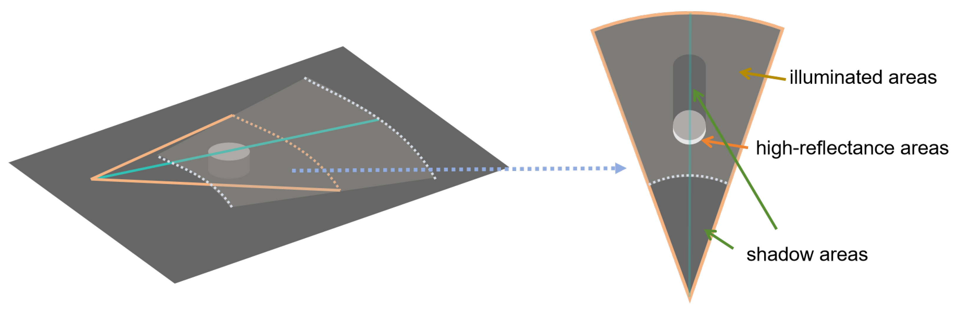
• Shadow Areas: These are regions where sound waves do not reach due to field-of-view limitations or obstacles blocking the path. Ideally, there should be no return signal, and these areas should appear completely black. However, background noise often causes speckle noise in these regions.
• Illuminated Areas: These are regions where the sound waves emitted by the FLS reach. Ideally, the structural features of objects within this area should be clearly reflected.
• High-Reflectance Areas: These regions have high reflectance due to the structure or density of objects. High-intensity and numerous reflected beams often result in phenomena such as ghosting.

Overall, an excellent FLS denoising algorithm should yield denoising results with clean shadow areas, clear illuminated areas, and precise high-reflectance areas. However, existing methods often fall short of achieving this.

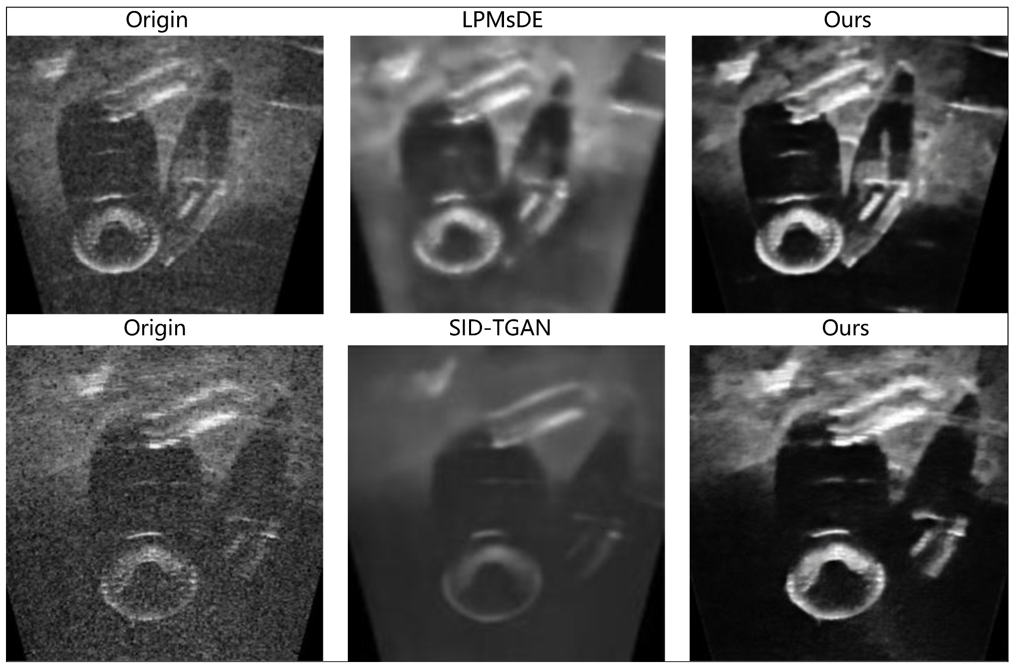
5.3.1. Qualitative Analysis

Using the open-source FLS object detection Marine Debris Dataset (WDD) [22], the effectiveness of the proposed denoising method is qualitatively analyzed. The proposed algorithm is compared with the latest traditional FLS denoising method (LPMsDE) [23] and a deep learning-based denoising method (SID-TGAN) [18]. As shown in the Figure 14, the scene includes multiple bottles and a tire. It is clear that the proposed denoising method has significant advantages in both noise removal and detail preservation.

Since the aforementioned algorithms are not open source and the denoising results provided in their respective papers are limited, we compare the proposed denoising algorithm with several classic open-source denoising algorithms, including bilateral filtering (BF) [24], non-local means (NLM) [25], and block-matching and 3D filtering (BM3D) [26]. It is clear that our method not only effectively removes noise but also significantly preserves high-frequency information. Additionally, we will make the inference results of all sonars in the WDD dataset open source, as detailed in the Data Availability Statement later in this paper.

As shown in the Figure 15, our proposed method continues to demonstrate significant advantages. The open source denoising methods, whether traditional spatial-domain or transform-domain approaches, exhibit very limited effectiveness on FLS data. Additionally, since these algorithms function essentially as low-pass filters, they often lead to the loss of texture information. In contrast, our method can accurately distinguish between the illuminated and shadowed areas in forward-looking sonar data, thereby significantly enhancing the quality of FLS data.

5.3.2. Quantitative Analysis

Quantitative evaluation of denoising algorithms in the field of the sonar is challenging due to the difficulty of obtaining clear, high-quality sonar image benchmarks. The simulated method proposed in this paper generates both noisy and noise-free FLS sonar data, effectively providing a data foundation for the quantitative evaluation of FLS denoising methods. When clear and noisy image pairs are available, we can evaluate the denoising performance of the model by measuring the differences between the denoised image and the clear image. The available evaluation metrics include the following:

• Peak Signal-to-Noise Ratio (PSNR) is one of the most widely used evaluation metrics in the field of image processing. PSNR is an engineering term that expresses the ratio between the maximum possible power of a signal and the destructive noise power that affects its accuracy. PSNR is usually expressed in logarithmic decibel units (dB). It is defined as follows for a high-quality reference image y and a noisy or denoised image x:

  $$PSN{R}_{x,y}=10{log}_{10}\left({\displaystyle \frac{2^n-1}{MS{E}_{x,y}}}\right)$$

  (8)

  where n represents the number of bits per pixel, and MSE is the mean square error calculated as follows:

  $$MS{E}_{x,y}={\displaystyle \frac{1}{m·n}}\sum _{i=1}^m\sum _{j=1}^n{(y_{i,j}-x_{i,j})}^2$$

  (9)

  where m and n represent the width and height of the image, respectively. The MSE is calculated by averaging the squared differences between corresponding pixels.
• The Structural Similarity Index (SSIM) is another widely used image similarity evaluation metric. Unlike PSNR, which evaluates pixel-by-pixel differences, SSIM measures structural information in the images, which is closer to how humans perceive visual information. Therefore, SSIM is often considered to better reflect a human evaluation of image quality. The core concept of structural similarity is based on the highly structured nature of natural images, where there is strong correlation between neighboring pixels, carrying structural information about the objects in the scene. The human visual system tends to extract structural information when observing images. Therefore, when designing image quality assessment metrics to measure image distortion, measuring structural distortion is particularly important. Given two image signals Y and X, the SSIM is defined as follows:

  $$SSIM\left(x,y\right)={\left[l\left(x,y\right)\right]}^{\alpha }{\left[c\left(x,y\right)\right]}^{\beta }{\left[s\left(x,y\right)\right]}^{\gamma },$$

  (10)
  In Equation (10), $l(x,y),c(x,y),s(x,y)$ represent luminance, contrast, and structure comparisons, respectively. The parameters $\alpha ,\beta ,\gamma$ adjust the relative importance of these three metrics, which are defined as follows:

  $$l\left(x,y\right)={\displaystyle \frac{2{\mu }_x{\mu }_y+C_1}{{\mu }_x^2+{\mu }_y^2+C_1}},c\left(x,y\right)={\displaystyle \frac{2{\sigma }_x{\sigma }_y+C_2}{{\sigma }_x^2+{\sigma }_y^2+C_2}},s\left(x,y\right)={\displaystyle \frac{{\sigma }_{xy}+C_3}{{\sigma }_x{\sigma }_y+C_3}}.$$

  (11)
  Here, ${\mu }_x,{\mu }_y,{\sigma }_x,{\sigma }_y$ denote the mean and standard deviation of x and y, respectively, and ${\sigma }_{xy}$ represents the covariance of x and y. $C_1,C_2,C_3$ are constants to maintain result stability. When computing the Structural Similarity Index (SSIM) between two images, a local window approach is typically used. Specifically, $N\times N$ windows are selected to evaluate SSIM within each window, moving them pixel by pixel until the entire image is covered. The overall SSIM between the two images is the average of these local SSIM values. A higher SSIM value indicates a higher similarity between the two images. Generally, SSIM and PSNR trends are similar, meaning that high PSNR values often correspond to high SSIM values.
• Gradient Magnitude Similarity Deviation (GMSD) assesses image quality by calculating image gradients, and it is known for its high accuracy and low computational cost. Natural images contain various local structures whose gradient magnitudes degrade to different extents when distorted. Changes in these local structures are crucial for image quality assessment. GMSD evaluates local image quality by calculating gradient magnitude similarity in local regions and then computing the standard deviation of these assessments to obtain the overall quality assessment. This approach comprehensively considers detailed local information and overall global perception, making the evaluation results more precise and comprehensive. When dividing an image into N local regions, GMSD is defined as follows:

  $$GMSD=\sqrt{{\displaystyle \frac{1}{N}}\sum _{i=1}^N{(GMS\left(i\right)-GMSM)}^2},$$

  (12)

  $$GMS\left(i\right)={\displaystyle \frac{2m_y\left(i\right)m_x\left(i\right)+c}{m_y^2\left(i\right)+m_x^2\left(i\right)+c}},$$

  (13)

  $$m_y\left(i\right)=\sqrt{{(y⨂h_r)}^2\left(i\right)+{(y⨂h_c)}^2\left(i\right)},$$

  (14)

  $$m_x\left(i\right)=\sqrt{{(x⨂h_r)}^2\left(i\right)+{(x⨂h_c)}^2\left(i\right)}.$$

  (15)
  GMS denotes gradient magnitude similarity, GMSM denotes its mean, $m_y,m_x$ denote the gradient magnitudes of the reference and degraded images, and $h_r,h_c$ are the Prewitt operators used to calculate image gradients.

We performed denoising on 1000 pairs of simulated FLS test data using classic open-source denoising methods and the proposed method. Some denoising results are shown in Figure 16.

The denoising capabilities of traditional methods are limited, as shown in the qualitative analysis results on real data. Next, the denoising results were evaluated using the three aforementioned metrics. As shown in

Table 2. Evaluation results of denoising effectiveness.

Method	Origin	Median	Gaussian	Bilateral	NLM	BM3D	Ours
PSNR ↑	17.64	17.76	17.76	17.90	17.73	16.65	20.77
SSIM ↑	0.68	0.69	0.69	0.69	0.69	0.69	0.79
GMSD ↓	0.22	0.19	0.20	0.19	0.21	0.19	0.18

, consistent with the qualitative analysis, these classic methods show very limited improvement in FLS data quality, whereas the proposed method demonstrates significant advantages.

5.3.3. Ablation Experiment

To validate the effectiveness of our proposed method, we conducted ablation experiments. Initially, adhering to traditional research methods, we employed the MDD dataset as noise-free images and subsequently added noise to generate noisy images, thus constructing a conventional training dataset. Subsequently, we performed ablation experiments by training the same denoising model with different datasets and loss functions.

As illustrated in Figure 17, training with the SimNFND dataset, constructed through the proposed simulation method, has significantly improved noise removal performance. Furthermore, with the application of the proposed NewLoss, the model’s accuracy in distinguishing between light and shadow has been enhanced.

Finally, we performed a qualitative analysis on the SimNFND test set. As demonstrated in

Table 3. Ablation experiment on the SimNFND dataset.

Method	PSNR ↑	SSIM ↑	GMSD ↓
OldData + L1loss	17.89705692	0.744666177	0.194743096
SimNFND + L1loss	20.16920049	0.7889269	0.188262191
SimNFND + Newloss	20.77546045	0.795312975	0.180447812

, the best results were obtained when using the simulated dataset and the new loss function. In summary, the proposed method has proven to be effective.

6. Conclusions

This study addresses the lack of noise-free ground truth in existing forward-looking sonar image denoising research by proposing an automated method based on existing large-scale RGBD datasets to generate forward-looking sonar data. Utilizing the Cycles ray tracing engine, we simulate ideal sonar imaging results, introducing various noise models to mimic the complex noise found in real-world sonar images, thus creating a diverse and realistic dataset of forward-looking sonar images. This enables the generation of paired noisy and noise-free sonar data, providing high-quality support for the development of sonar image processing algorithms. We also optimize the loss function and training methods of the Restormer denoising model, thereby achieving precise noise removal and significantly improving detail retention and denoising capabilities compared to previous work.

Future research will focus on further enhancing simulated data quality and synthesizing data that are challenging or impossible to collect directly using simulation methods. Additionally, exploring methods to align RGBD cameras with real FLS sonar will be a priority. This will facilitate the effective application of deep learning algorithms to sonar image denoising, target detection, and other areas, improving the accuracy and generalization of various algorithms. Additionally, integrating sonar technology with other underwater sensing technologies, such as optical and LiDAR, will significantly enhance the overall performance and reliability of underwater environment perception. This will provide robust technical support for the exploration and development of ocean resources.

References

1. Greene, A.; Rahman, A.F.; Kline, R.; Rahman, M.S. Side scan sonar: A cost-efficient alternative method for measuring seagrass cover in shallow environments. Estuar. Coast. Shelf Sci. 2018, 207, 250–258. [Google Scholar] [CrossRef]
2. Arshad, M.R. Recent advancement in sensor technology for underwater applications. Indian J. Mar. Sci. 2009, 38, 267–273. [Google Scholar]
3. Hurtós, N.; Palomeras, N.; Carrera, A.; Carreras, M. Autonomous detection, following and mapping of an underwater chain using sonar. Ocean Eng. 2017, 130, 336–350. [Google Scholar] [CrossRef]
4. Henriksen, L. Real-time underwater object detection based on an electrically scanned high-resolution sonar. In Proceedings of the IEEE Symposium on Autonomous Underwater Vehicle Technology (AUV’94), Cambridge, MA, USA, 19–20 July 1994; pp. 99–104. [Google Scholar]
5. Gu, J.-H.; Joe, H.-G.; Yu, S.-C. Development of image sonar simulator for underwater object recognition. In Proceedings of the 2013 OCEANS, San Diego, CA, USA, 10–13 June 2013; IEEE: Piscataway, NJ, USA, 2013; pp. 1–6. [Google Scholar]
6. Kwak, S.; Ji, Y.; Yamashita, A.; Asama, H. Development of acoustic camera-imaging simulator based on novel model. In Proceedings of the 2015 IEEE 15th International Conference on Environment and Electrical Engineering (EEEIC), Rome, Italy, 10–13 June 2015; IEEE: Piscataway, NJ, USA, 2015; pp. 1719–1724. [Google Scholar]
7. Cerqueira, R.; Trocoli, T.; Neves, G.; Oliveira, L.; Joyeux, S.; Albiez, J.; Center, R.I. Custom shader and 3D rendering for computationally efficient sonar simulation. In Proceedings of the 29th Conference on Graphics, Patterns and Images-SIBGRAPI, Sao Paulo, Brazil, 4–7 October 2016. [Google Scholar]
8. Cerqueira, R.; Trocoli, T.; Albiez, J.; Oliveira, L. A rasterized ray-tracer pipeline for real-time, multi-device sonar simulation. Graph. Model. 2020, 111, 101086. [Google Scholar] [CrossRef]
9. Potokar, E.; Lay, K.; Norman, K.; Benham, D.; Neilsen, T.B.; Kaess, M.; Mangelson, J.G. HoloOcean: Realistic sonar simulation. In Proceedings of the 2022 IEEE/RSJ International Conference on Intelligent Robots and Systems (IROS), Kyoto, Japan, 23–27 October 2022; pp. 8450–8456. [Google Scholar]
10. Zhengguo, S.; Chunhui, Z.; Jian, W. Application of multi-resolution analysis in sonar image denoising. J. Syst. Eng. Electron. 2008, 19, 1082–1089. [Google Scholar] [CrossRef]
11. Isar, A.; Moga, S.; Isar, D. A new denoising system for SONAR images. EURASIP J. Image Video Process. 2009, 2009, 173841. [Google Scholar] [CrossRef]
12. Wang, X.; Liu, A.; Zhang, Y.; Xue, F. Underwater acoustic target recognition: A combination of multi-dimensional fusion features and modified deep neural network. Remote Sens. 2019, 11, 1888. [Google Scholar] [CrossRef]
13. Jin, Y.; Ku, B.; Ahn, J.; Kim, S.; Ko, H. Nonhomogeneous noise removal from side-scan sonar images using structural sparsity. IEEE Geosci. Remote Sens. Lett. 2019, 16, 1215–1219. [Google Scholar] [CrossRef]
14. Vishwakarma, A. Denoising and inpainting of sonar images using convolutional sparse representation. IEEE Trans. Instrum. Meas. 2023, 72, 5007709. [Google Scholar] [CrossRef]
15. Cho, H.; Yu, S.-C. Real-time sonar image enhancement for AUV-based acoustic vision. Ocean Eng. 2015, 104, 568–579. [Google Scholar] [CrossRef]
16. Kim, J.; Song, S.; Yu, S.-C. Denoising auto-encoder based image enhancement for high resolution sonar image. In Proceedings of the 2017 IEEE Underwater Technology (UT), Busan, Republic of Korea, 21–24 February 2017; pp. 1–5. [Google Scholar]
17. Shen, P.; Zhang, L.; Wang, M.; Yin, G. Deeper super-resolution generative adversarial network with gradient penalty for sonar image enhancement. Multimed. Tools Appl. 2021, 80, 28087–28107. [Google Scholar] [CrossRef]
18. Zhou, X.; Tian, K.; Zhou, Z.; Ning, B.; Wang, Y. SID-TGAN: A Transformer-Based Generative Adversarial Network for Sonar Image Despeckling. Remote Sens. 2023, 15, 5072. [Google Scholar] [CrossRef]
19. Lu, Z.; Zhu, T.; Zhou, H.; Zhang, L.; Jia, C. An image enhancement method for side-scan sonar images based on multi-stage repairing image fusion. Electronics 2023, 12, 3553. [Google Scholar] [CrossRef]
20. Abraham, D.A.; Lyons, A.P. Novel physical interpretations of k-distributed reverberation. IEEE J. Ocean. Eng. 2002, 27, 800–813. [Google Scholar] [CrossRef]
21. Randall, Y.; Treibitz, T. Flsea: Underwater visual-inertial and stereo-vision forward-looking datasets. arXiv 2023, arXiv:2302.12772. [Google Scholar]
22. Singh, D.; Valdenegro-Toro, M. The Marine Debris Dataset for Forward-Looking Sonar Semantic Segmentation. In Proceedings of the 2021 IEEE/CVF International Conference on Computer Vision Workshops (ICCVW), Montreal, BC, Canada, 11–17 October 2021; pp. 3734–3742. [Google Scholar]
23. Wang, Z.; Li, Z.; Teng, X.; Chen, D. LPMsDE: Multi-Scale Denoising and Enhancement Method Based on Laplacian Pyramid Framework for Forward-Looking Sonar Image. IEEE Access 2023, 11, 132942–132954. [Google Scholar] [CrossRef]
24. Tomasi, C.; Manduchi, R. Bilateral filtering for gray and color images. In Proceedings of the Sixth International Conference on Computer Vision, Washington, DC, USA, 4–7 January 1998; pp. 839–846. [Google Scholar]
25. Dabov, K.; Foi, A.; Katkovnik, V. Image denoising by sparse 3-D transform-domain collaborative filtering. IEEE Trans. Image Process. 2007, 16, 2080–2095. [Google Scholar] [CrossRef] [PubMed]
26. Buades, A.; Coll, B.; Morel, J.-M. Non-local means denoising. Image Process. Line 2011, 1, 208–212. [Google Scholar] [CrossRef]
Figure 1. Dataset construction illustration.
Remotesensing 16 02815 g001
Figure 2. Point cloud from RGBD conversion.
Remotesensing 16 02815 g002
Figure 3. RGBD data and rendering results.
Remotesensing 16 02815 g003
Figure 4. Top view with reflective intensity point cloud.
Remotesensing 16 02815 g004
Figure 5. Background noise simulation schematic diagram. (a) Noise-free FLS simulation image; (b) Background noise FLS simulation image; (c) Actual FLS image.
Remotesensing 16 02815 g005
Figure 6. Spread noise simulation schematic diagram. (a) Noise-free FLS simulation image; (b) Spread noise with K-distribution; (c) Spread noise with our method; (d) Actual FLS image.
Remotesensing 16 02815 g006
Figure 7. Multipath noise simulation schematic diagram. (a) Noise-free FLS simulation image; (b) Multipath noise FLS simulation image; (c) Actual FLS image.
Remotesensing 16 02815 g007
Figure 8. Azimuthal Artifacts simulation schematic diagram. (a) Noise-free FLS simulation image; (b) FLS Simulation image with Azimuthal Artifacts; (c) Actual FLS image.
Remotesensing 16 02815 g008
Figure 9. Architecture of Restormer for high-resolution image restoration.
Remotesensing 16 02815 g009
Figure 10. Diagram of shadow region discrimination. (a) Original image; (b) threshold segmentation.
Remotesensing 16 02815 g010
Figure 11. Comparison of FLS simulation data with real data. (ad) RGB, rendered, simulated, and real sonar images of chains. (eh) RGB, rendered, simulated, and real sonar images of tires.
Remotesensing 16 02815 g011
Figure 12. Simulation FLS data generation.
Remotesensing 16 02815 g012
Figure 13. Schematic diagram of FLS imaging.
Remotesensing 16 02815 g013
Figure 14. Comparison with the latest FLS denoising methods.
Remotesensing 16 02815 g014
Figure 15. Comparison with the open source denoising methods on WDD.
Remotesensing 16 02815 g015
Figure 16. Comparison with the open source denoising methods on simulated data.
Remotesensing 16 02815 g016
Figure 17. Ablation experiment on the WDD dataset.
Remotesensing 16 02815 g017