Modeling Spatio-Temporal Rainfall Distribution in Beni–Irumu, Democratic Republic of Congo: Insights from CHIRPS and CMIP6 under the SSP5-8.5 Scenario

Abstract

In light of the lack of ground-based observations, this study utilizes reanalysis data from the CHIRPS database and CMIP6 models under the SSP5-8.5 scenario to predict future rainfall in the Beni–Irumu region of eastern DR Congo. The use of reanalysis data offers a viable method for understanding historical and future climate trends in regions with limited ground data. Using a spatial resolution of 0.05°, selected general circulation models (GCMs) were downscaled to CHIRPS data. Analysis of historical rainfall data over 32 years reveals spatial disparities, with high-altitude regions like Mount Stanley experiencing higher annual mean rainfall (1767.87 ± 174.41 mm) compared to lower areas like Kasenyi (863.65 ± 81.85 mm), in line with orographic effects. Future projections under the SSP5-8.5 scenario indicate significant decreases in rainfall for areas such as Oicha (−565.55 mm) in the near term, while regions like Kasindi/Yihunga exhibit moderate decrease (−58.5 mm). In the mid-term, some areas show signs of recovery, with Bulongo experiencing a minor decrease (−21.67 mm), and Kasindi/Yihunga (+152.95 mm) and Kyavinyonge (+71.11 mm) showing increases. Long-term projections suggest overall improvements, with most areas experiencing positive rainfall differences; however, persistent challenges remain in Oicha (−313.82 mm). These findings highlight the dynamic impacts of climate change on rainfall distribution in the Beni–Irumu region, underscoring the need for targeted interventions to address the varied impacts, especially in vulnerable regions like Oicha.

1. Introduction

Since the 1950s, the global climate system has experienced profound changes attributed to global warming, resulting in an increased susceptibility to natural disasters such as floods and droughts, which in turn affect agricultural economies [1]. Climate change’s role in intensifying the impacts of natural disasters, along with its implications for mitigation and adaptation strategies, has garnered significant attention [2]. Accurately predicting future climate changes at a regional level is crucial for effectively addressing and adapting to the challenges posed by climate change [3]. To achieve this, it is important to study recent climate variations and make projections about future changes. Such knowledge is essential for developing adaptation strategies that can specifically cater to the needs of a particular region [4]. One area of focus has been the analysis of rainfall trends, which is crucial for various sectors like water resource management, policy formulation, and disaster preparedness [5]. Data scarcity challenges our comprehensive understanding of climate and hydrological processes, necessitating reliable climate information for crafting climate-resilient interventions [6].

In the Democratic Republic of Congo, there is a scarcity of climate data tailored to local conditions in basins and territories. This knowledge gap is especially conspicuous in the Beni–Irumu region, which features diverse topographic aspects. Despite existing studies examining rainfall trends in Beni city, one of the region’s cities [7,8], significant constraints persist. These constraints primarily stem from a reliance on limited rainfall station data, which often results in overlooked, finer-scale variations. Additionally, the lack of spatial rainfall distribution information hinders a comprehensive understanding of rainfall patterns in the region.

To address these gaps, the use of satellite-derived precipitation datasets combined with ground-based data offers a more comprehensive understanding of rainfall patterns [9,10]. Reanalysis rainfall datasets, like CHIRPS, offer improved precision and resolution, particularly in regions with limited observational data. Studies have demonstrated the accuracy of CHIRPS data in tropical Africa, including the Eastern Africa Rift Valley and Congo Basin. For instance, [11] validated CHIRPS in Northeast Brazil, showing a strong correlation with ground observations (r = 0.94). Ref. [12] found CHIRPS to perform well in Central East Africa, with good correlation over various temporal scales. Additionally, [13] validated CHIRPS in Eastern Africa, confirming its superiority over other satellite products like ARC2. Ref. [14] demonstrated the reliability of CHIRPS in predicting rainfall in Kenya. Ref. [15] assessed CHIRPS data for spatio-temporal precipitation variability in Uganda. Ref. [16] evaluated CHIRPS data accuracy in Tanzania, finding it well correlated with ground observations.

Moreover, assessing climate change impacts requires relevant climate projections at various scales [17,18]. However, challenges persist in selecting appropriate general circulation models due to uncertainties [19].

Advancements in climate modeling, exemplified by CMIP6, offer solutions [20]. CMIP6 models feature higher resolutions, enhanced parameters, and additional components [21,22]. Notably, CMIP6’s utilization of socioeconomic pathways (SSPs) instead of radiative forcing values offers more realistic future scenarios. Moreover, CMIP6 emphasizes model intercomparison to address biases and processes [23,24]. Focusing on SSP5, the “Fossil-Fueled Development” scenario, is strategic due to its attributes and consequences [25,26]. SSP5 depicts a future where fossil fuel use remains central for energy and economic growth, highlighting its potential impacts on emissions, environment, and climate [25]. The trajectory’s emphasis on fossil fuels necessitates investigation of its link to global warming [26] and exploring SSP5 holds policy importance for informed decision-making. This choice also prompts examination of societal and economic dynamics, addressing trade-offs between short-term growth and long-term sustainability [27]. Analyzing SSP5 contributes to cleaner energy discussions and aligns with climate goals.

This research aims to evaluate historical and projected spatio-temporal rainfall distribution over the Beni–Irumu region using recent climate models under SSP5-8.5. It seeks to overcome the lack of documented local climate information, by leveraging advancements in reanalysis data from the CHIRPS (Climate Hazards Group InfraRed Precipitation with Stations) database and investigating climate change impacts on this climatologically diverse area using CMIP6 models. The study’s findings will provide crucial insights into the region’s climate dynamics, enabling informed decision-making for resilience and adaptation strategies.

2. Materials and Methods

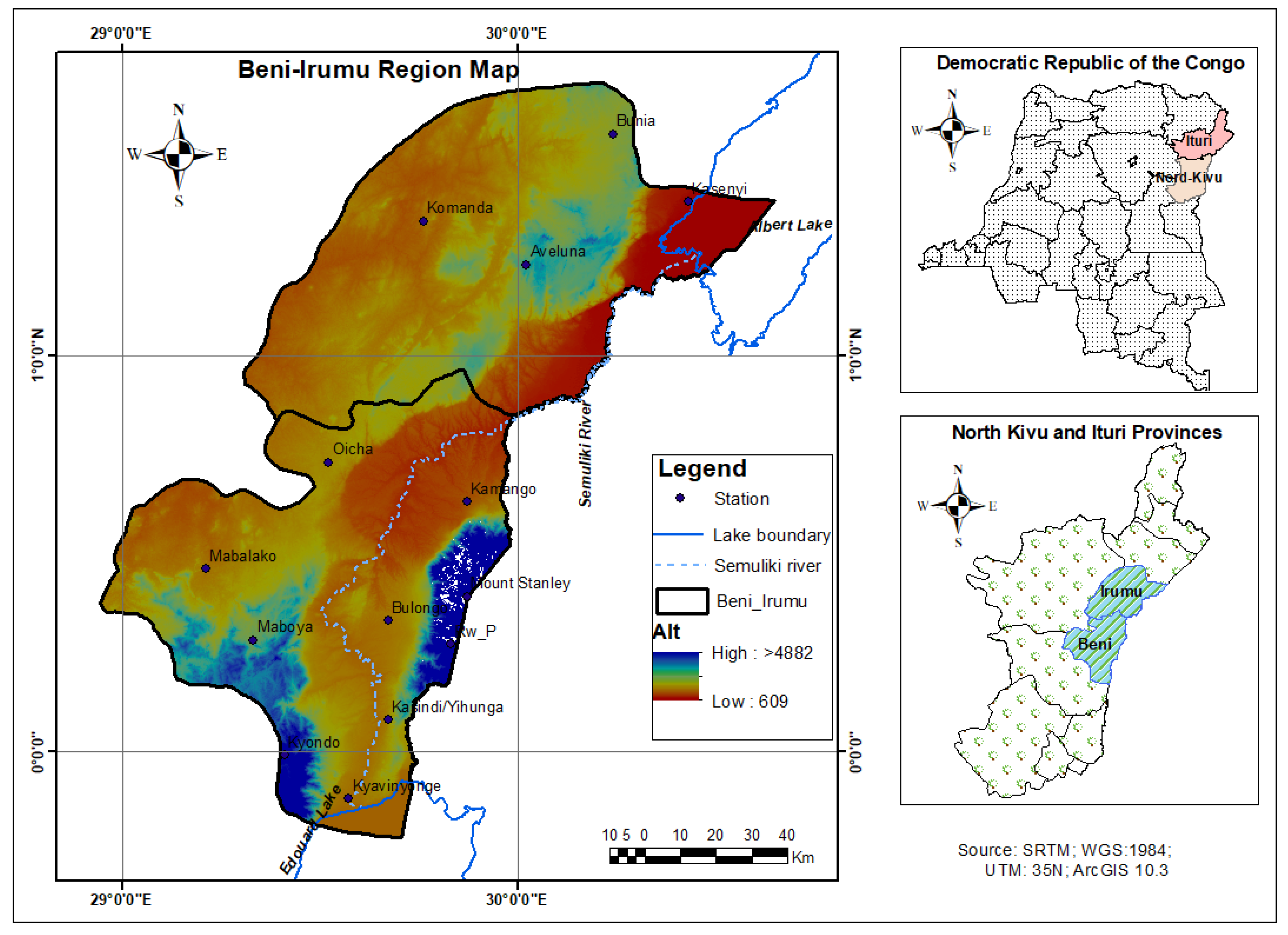
2.1. Study Area

The Beni–Irumu region, situated in the eastern Democratic Republic of Congo, spans the territories of Beni and Irumu, located, respectively, in the North Kivu and Ituri Provinces. Geographically, it extends between longitudes 29°0′0″E and 30°0′0″E, and latitudes 0°0′0″N and 1°0′0″N (Figure 1). The Beni territory is subdivided into four distinct subregions: Beni–Mbau, Watalinga, Ruwenzori, and Bashu. The Irumu territory consists of twelve subregions: Andisoma, Babelebe, Baboa–Bokoe, Bahema d’Irumu, Bahema–Mitego, Bahema–Boga, Banyari Tchabi, Basili, Mobala, Walendu Bindi, Walese Vonkutu, and Bahema–Sud. Topographically, Beni–Irumu features a diverse elevation range from 609 m to more than 4882 m, with the highest elevations found on Mount Ruwenzori (>4882 m) and the southern mountains of the Bashu Chiefdom (up to 3047 m). The lowest elevations occur along the Semuliki River, particularly in the Kasenyi area (Figure 1). Hydrologically, the region is dominated by the Semuliki River, which connects Lake Edward to the south and Lake Albert to the northeast (Figure 1). Traditional agricultural practices are central to the region’s economy, serving as the primary livelihood source for the local population. Given the reliance on rainfall for agriculture and the area’s varied topography and climatic conditions, understanding the region’s rainfall patterns is crucial.

2.2. Data Collection

Daily reanalysis rainfall data for the study area were obtained from the CHIRPS (Climate Hazards Group InfraRed Precipitation with Stations) database. CHIRPS provides freely accessible daily climate data with a gridded spatial resolution of 0.05°, covering a quasi-global range (50°S–50°N, 180°E–180°W) [28]. This database undergoes a multi-stage synthesis process that integrates satellite records and in situ station data, ensuring its reliability and versatility for scientific research, including climate studies, hydrological modeling, and agricultural assessments. Developed to support the United States Agency for International Development Famine Early Warning Systems Network (FEWS NET), CHIRPS incorporates methodologies from successful thermal infrared (TIR) precipitation products, such as NOAA’s Rainfall Estimate (RFE2) and African Rainfall Climatology [29], along with the University of Reading’s TAMSAT African Rainfall Climatology and Time series (TARCAT). By leveraging the Tropical Rainfall Measuring Mission Multi-Satellite Precipitation Analysis version 7 (TMPA 3B42 v7), CHIRPS calibrates global cold cloud duration (CCD) rainfall estimates, enhancing its accuracy [28]. The datasets, for 14 virtual stations (Figure 1), used in this study span from 1983 to 2016, providing a robust foundation for analyzing climate and weather dynamics at detailed spatial and temporal scales. The virtual stations selected have been named using the names of the locations, corresponding to their geographical coordinates, as shown in

Table 1. Latitude, longitude, altitude, and operational periods of meteorological stations.

ID	Observed	Latitude	Longitude (East)	Altitude (m)
1	Aveluna	1.23°N	30.02	1564
2	Bulongo	0.33°N	29.67	971
3	Bunia	1.56°N	30.24	1239
4	Kamango	0.63°N	29.87	859
5	Kasenyi	1.39°N	30.43	638
6	Kasindi/Yihunga	0.08°N	29.67	1018
7	Komanda	1.34°N	29.76	928
8	Kyavinyonge	−0.12°S	29.57	924
9	Kyondo	−0.01°S	29.41	2244
10	Mabalako	0.46°N	29.21	962
11	Maboya	0.28°N	29.33	1407
12	Oicha	0.73°N	29.52	1041
13	Mount Stanley	0.39°N	29.87	>4765
14	Rw_P	0.27°N	29.83	3473

.

For climate projection, rainfall data from the GFDL-ESM4 and INM-CM5-0 models were sourced from the Coupled Model Intercomparison Project Phase 6 (CMIP6) database, ensuring access to reliable and standardized climate model outputs. These models were chosen based on their resolution capabilities. The GFDL-ESM4 model, developed by the National Oceanic and Atmospheric Administration’s Geophysical Fluid Dynamics Laboratory, provides detailed information on various climate variables, including precipitation, with a resolution of 50 km for key components such as the ocean, ocean biogeochemistry, and sea ice [30]. Similarly, the INM-CM5-0 model, developed by the Institute for Numerical Mathematics at the Russian Academy of Science, offers high-resolution data for precipitation, with a resolution of 50 km for ocean and sea ice components [31]. The study used the SSP5-8.5 scenario from the Shared Socioeconomic Pathways (SSPs), representing a high-forcing “fossil-fueled” development pathway. Rainfall data from these models were accessed via the CMIP6 web data portal, ensuring consistency by exclusively using the ‘r1i1p1f1’ variant, denoting the first realization, initialization, physics, and forcing.

2.3. Processing and Analysis

2.3.1. Downscaling and Bias Correction

The downscaling process employed a statistical approach, with bias correction performed using the distribution mapping (DM) technique. This method provided the spatial refinement and detail needed for localized climate impact assessments. In the DM technique, the distribution function of the simulated general circulation model (GCM) data is adjusted to match that of the observed data. This adjustment modifies the mean, standard deviation, and quantiles while preserving extreme values. The approach assumes that both the observed and model-simulated raw data follow the same distribution, thereby reducing unnecessary biases [32]. For precipitation, the gamma distribution function with shape parameter α and scale parameter β was utilized. This distribution function has been verified to be effective and is expressed in distribution 1 (Equation (1)), where x represents the observed variable, ⎾(.) is the gamma function, α is the form parameter, and β is the scale parameter.

$$f\gamma \left(x|\alpha ,\beta \right)=x^{\alpha -1}\times {\displaystyle \frac{1}{{\beta }^{\alpha }\times \lceil \left(\alpha \right)}}\times e^{{\displaystyle \frac{-x}{\beta }}};x\ge 0, \alpha , \beta >0$$

(1)

The bias correction for precipitation is performed using distribution 2 (Equation (2)), known as the LOCI-corrected precipitation data, where Fγ () and $F_{\gamma }^{-1}$( ) are the gamma CDF (cumulative distribution function) and its inverse; α_LOCI,m and β_LOCI,m are the fitted gamma parameters for the LOCI-corrected precipitation in a given month m; and α_obs,m and β_obs,m are the fitted gamma parameters for observed data.

$$P_{cor,m,d}=F_{\gamma }^{-1}(F_{\gamma }(P_{LOCI,m,d}|{\alpha }_{LOCI,m},{\beta }_{LOCI,m})|{\alpha }_{obs,m},{\beta }_{obs,m})$$

(2)

The bias correction has been we perform on individual models before averaging them. This strategy aims to ensure that each model’s biases are addressed independently, thereby improving the overall accuracy of our findings.

2.3.2. GCM Performance in Simulating Rainfall

To rigorously evaluate the accuracy and performance of the selected general circulation models (GCMs), the study used a comparison of observed and simulated rainfall distribution maps, along with some statistical metrics. Let n represent the number of observations, Pi the simulated value, and Oi the observed value. Mean absolute error (MAE) quantified the average magnitude of errors in a set of predictions (Equation (3)) [33]. Percent bias (Pbias) indicated the average tendency of the predicted values to be systematically larger or smaller than the observed values (Equation (4)).

$$MAE={\displaystyle \frac{1}{n}}{{\displaystyle \sum }}_{i=1}^n\left|P_i-O_i\right|$$

(3)

$$Pbias=100\times {\displaystyle \frac{{{\displaystyle \sum }}_{i=1}^n\left(P_i-O_i\right)}{{{\displaystyle \sum }}_{i=1}^n{O}_i}}$$

(4)

To improve the reliability of rainfall projections and reduce the uncertainty inherent in any single model’s predictions, the study employed the “model ensemble” approach [34]. This method involved averaging the outputs of the two selected GCMs, GFDL-ESM4 and INM-CM5-0, to create a composite dataset that leverages the strengths of both models.

2.3.3. Spatio-Temporal Rainfall Patterns Analysis

The rainfall patterns assessment spanned three distinct periods: a 32-year baseline (historical) period from 1983 to 2014, and three 25-year intervals representing the near term (2026–2050), midterm (2051–2075), and long term (2076–2100). Analyses were conducted using Originlab and ArcGIS 10.3 softwares. A comprehensive investigation into historical and projected trends was undertaken using robust statistical method, the Mann–Kendall test. This methodical assessment has been previously endorsed by researchers [35,36,37] for trend detection in climate phenomena. This non-parametric technique evaluates correlations between time and rainfall data, with detection of statistically significant trends relying on the Z-value. A significance level of 0.05 was employed, yielding p-values for each analyzed time series.

For spatial rainfall distribution mapping, the inverse distance weighting (IDW) algorithm was used. This technique interpolates point-based rainfall observations to generate continuous surfaces of precipitation across the study area. The IDW algorithm calculates the value of each grid cell in the interpolated surface based on the weighted average of observed rainfall values from nearby gauge locations, with weights inversely proportional to the distance from the cell to the gauges.

The standardized precipitation index (SPI), which denotes the deviation of precipitation from the long-term mean standardized by the standard deviation, was also calculated using Equation (5), where ${\chi }_i, {\chi }_{m }$ and σ are, respectively, the value for the year or month i, the average, and the standard deviation of the time series.

$$SPI={\displaystyle \frac{{\chi }_i-{\chi }_m}{\mathsf{\sigma }}}$$

(5)

The interpretation was performed according to the classification shown in

Table 2. The classification system of the SPI values.

SPI	Drought Sequences
2.0+	extremely wet
1.5 to 1.99	very wet
1.0 to 1.49	moderately wet
−0.99 to 0.99	near normal
−1.0 to −1.49	moderately dry
−1.5 to −1.99	severely dry
−2 and less	extremely dry

, as used by [38].

3. Results

3.1. Ensemble Model Accuracy and Performance in Simulating Rainfall Patterns

Comparing the observed and simulated rainfall distribution maps (Figure 2) highlights the performance of the Ensemble model in capturing spatial patterns of precipitation. The analysis shows a close alignment between the observed CHIRPS data and the simulated outputs.

The mean observed rainfall of 1306.13 mm closely matches the mean simulated rainfall of 1315.56 mm, demonstrating the model’s ability to capture the overall trend. The mean absolute error (MAE) of 9.42 mm signifies a relatively small average absolute deviation between observed and predicted values, suggesting good accuracy. Despite a percent bias (Pbias) of 0.72%, indicating a slight tendency to overestimate rainfall, this bias is minimal. These findings suggest that the model performs well in simulating rainfall, providing valuable insights into precipitation patterns.

3.2. Spatio-Temporal Distribution of Rainfall under Different Periods

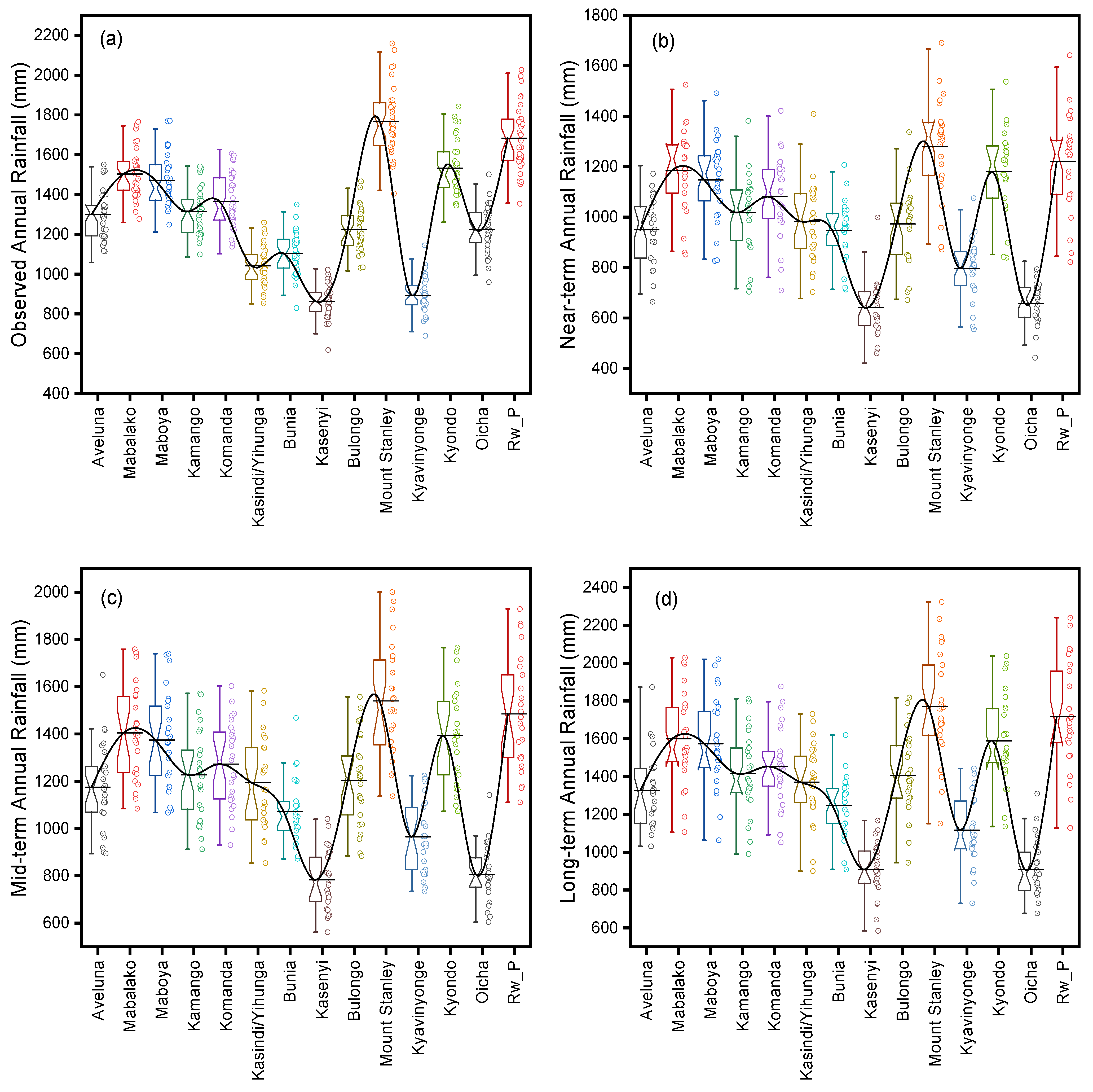
3.2.1. Annual Rainfall Distribution

The analysis of rainfall distribution over the Beni–Irumu region highlights significant spatial and temporal variations. Over the past 32 years, the spatial distribution of rainfall shows low values in Kyavinyonge, Kasindi/Yihunga, Bunia, and Kasenyi, while higher amounts are recorded in the Mount Stanley, Kyondo, Maboya, and Mabalako areas (Figure 3a). Future projections under the high-forcing “fossil-fueled” development pathway indicate that the spatial distribution will remain nearly the same (Figure 3b–d).

Historically, CHIRPS observed data indicates that Mount Stanley experiences the highest annual mean rainfall with 1767.87 ± 174.41 mm, while Kasenyi records the lowest with 863.65 ± 81.85 mm (Figure 4a). In the near term, projections show that Kasenyi will have the lowest annual mean rainfall at 641.11 ± 110.32 mm, while Mount Stanley will continue to have the highest at 1769.74 ± 193.48 mm (Figure 4b). In the midterm, the trend continues with Kasenyi’s rainfall increasing to 782.85 ± 124.92 mm and Mount Stanley experiencing a decrease to 1539.95 ± 234.87 mm, still marking the extremes for this period (Figure 4c). Long-term projections indicate that Kasenyi’s rainfall will rise to 909.54 ± 139.49 mm, maintaining its position as the area with the lowest mean rainfall, while Mount Stanley’s rainfall will revert to 1769.74 ± 284.67 mm, consistently being the area with the highest mean rainfall (Figure 4d).

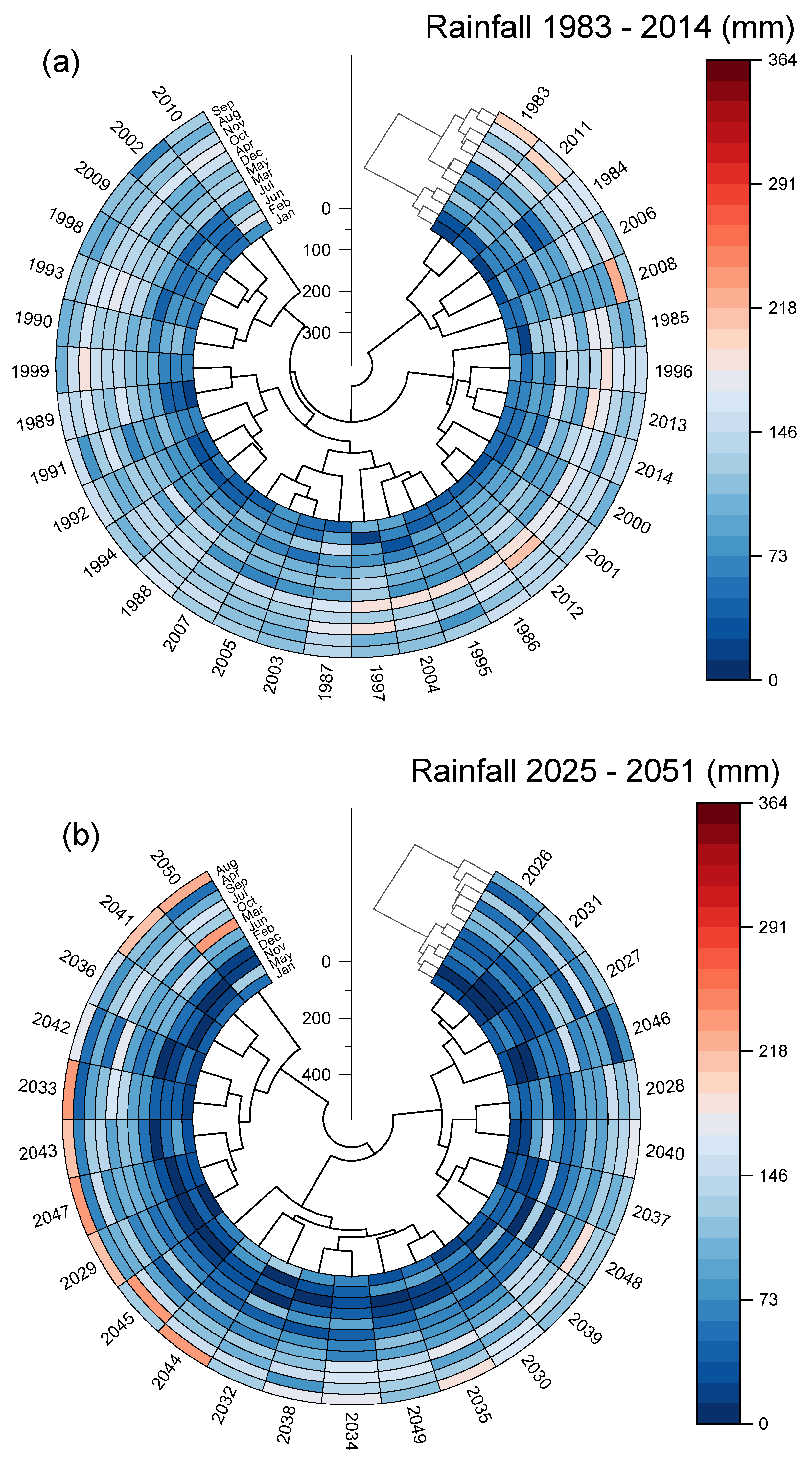
3.2.2. Monthly Rainfall Distribution

Analyzing the historical data (Figure 5a) over the course of 32 years, the months of June, July, March, January, and February recorded the lowest rainfall values. In contrast, the highest precipitation levels were observed in August, September, November, October, and April. For future projections, perturbations in rainfall distribution are expected under the SSP5-8.5 scenario. In the near future (Figure 5b), January, May, November, December, and February are expected to receive less precipitation, while August and April are projected to have the highest rainfall values.

In the midterm (Figure 6a), November, May, and December are expected to receive the lowest rainfall values, whereas August, July, and September are projected to experience the highest values over time. For the long term (Figure 6b), April, May, and November are expected to observe lower rainfall values, while August, July, September, and February are anticipated to receive the highest rainfall amounts.

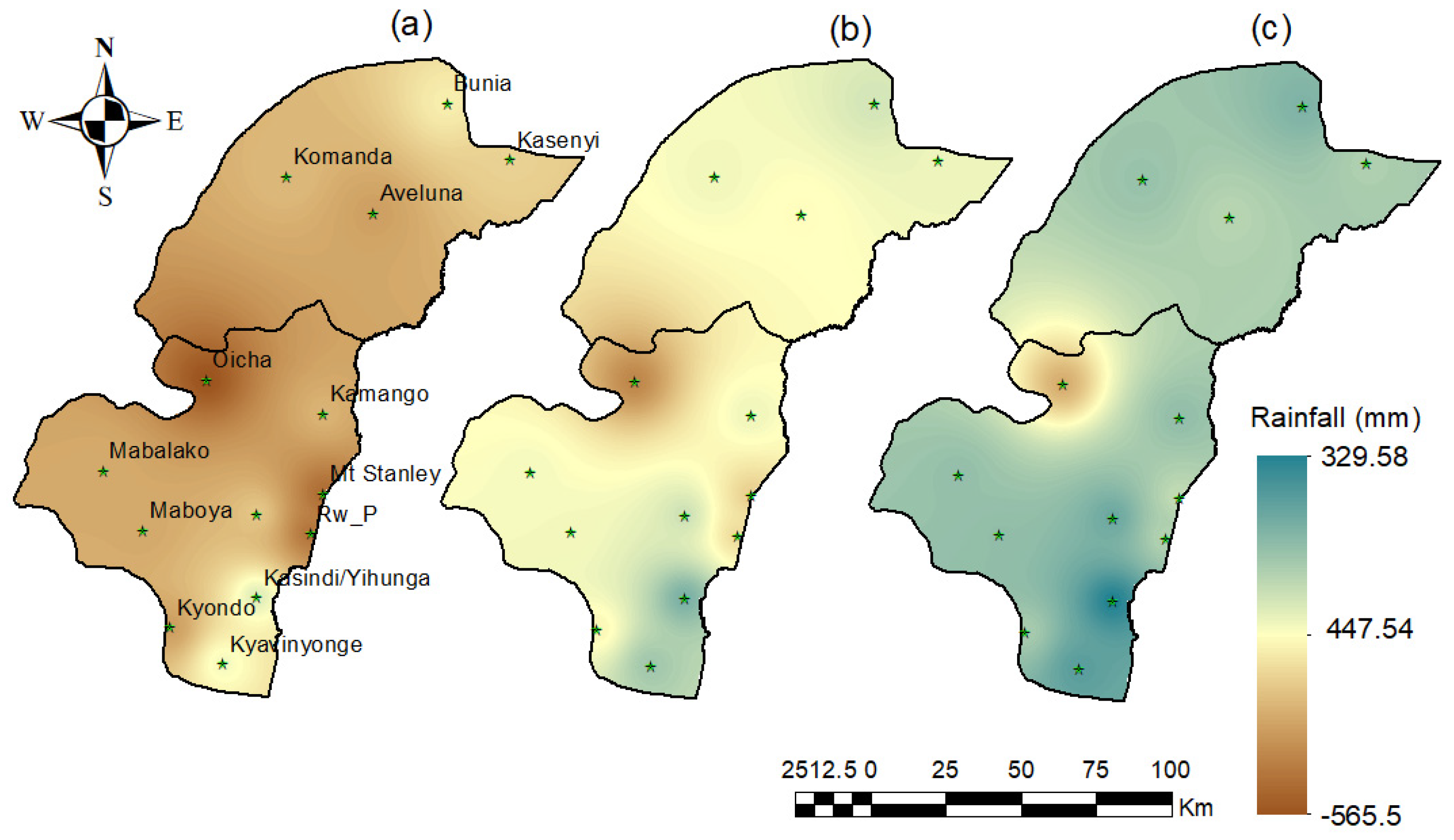
3.3. Projected Climate Signal and Rainfall Distribution Variations under SSP5-8.5 Scenario

The climate signal, derived from the difference between annual projected and historical rainfall, reveals notable trends and variations across the Beni–Irumu region under the SSP5-8.5 scenario. In the near term, significant decreases in rainfall are projected for Oicha (−565.55 mm), with moderate decreases in areas such as Bulongo (−251.25 mm), Kamango (−296.58 mm), and Maboya (−323.45 mm). Kasindi/Yihunga experiences the smallest decrease (−58.5 mm), indicating relative stability (Figure 7a and Table S1). By the midterm, Bulongo (−21.67 mm) shows the smallest decrease, suggesting a slight recovery, while Kasindi/Yihunga (152.95 mm) and Kyavinyonge (71.11 mm) exhibit notable increases. However, Oicha remains significantly negative (−417.48 mm), indicating a persistent reduction (Figure 7b and Table S1). Long-term projections show an overall recovery, with most areas experiencing positive differences, with Kasindi/Yihunga (329.7 mm) expected to obtain the highest value, while Mount Stanley (1.87 mm) and Aveluna (26.36 mm) experience minor increases, indicating stabilization (Figure 7c and Table S1). Despite this, Oicha still records a negative difference (−313.82 mm), suggesting ongoing challenges. These projections highlight the dynamic nature of climate impacts on rainfall distribution in the Beni–Irumu region, with some areas experiencing significant declines in the near- and midterm, followed by notable recoveries in the long term.

3.4. Rainfall Annual Trend Analysis

The rainfall trend analysis reveals distinct patterns across different timescales in the Beni–Irumu region (Figure 8). Over the past 32 years, some regions like Kasenyi, Komanda, Aveluna, Maboya, Mount Stanley, and Mabalako have experienced negative trends, while other regions have shown positive trends. However, these decreases or increases are not statistically significant.

For future projections, under the SSP5-8.5 scenario, only positive trends are expected. In the near term, Komanda and Kyavinyonge are projected to experience significant positive trends. In the midterm, several regions, including Aveluna, Maboya, Kamango, Bunia, Bulongo, Mount Stanley, Kyondo, and Oicha, are expected to see an increase in rainfall over time. In the long term, no significant trends are anticipated. These projections highlight the varying nature of rainfall trends in the Beni–Irumu region under the SSP5-8.5 scenario, with notable increases in certain areas in the near- and midterm but stabilization in the long term.

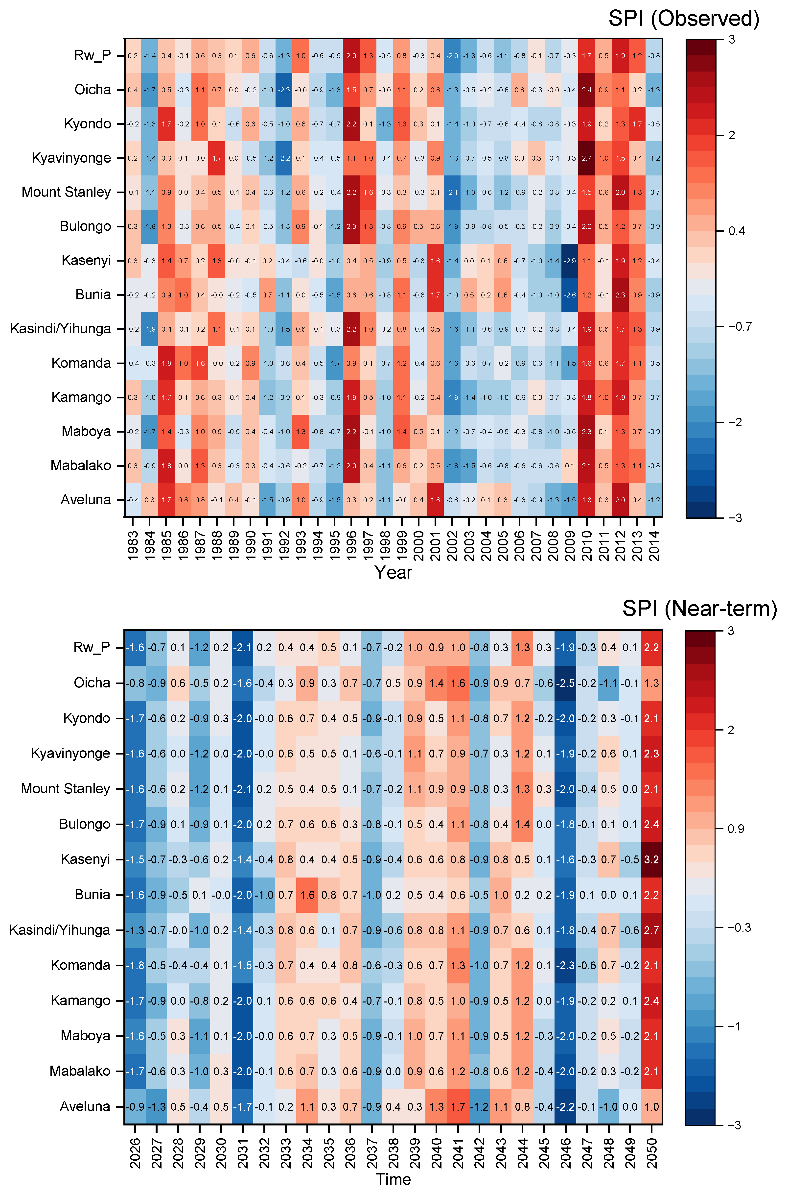
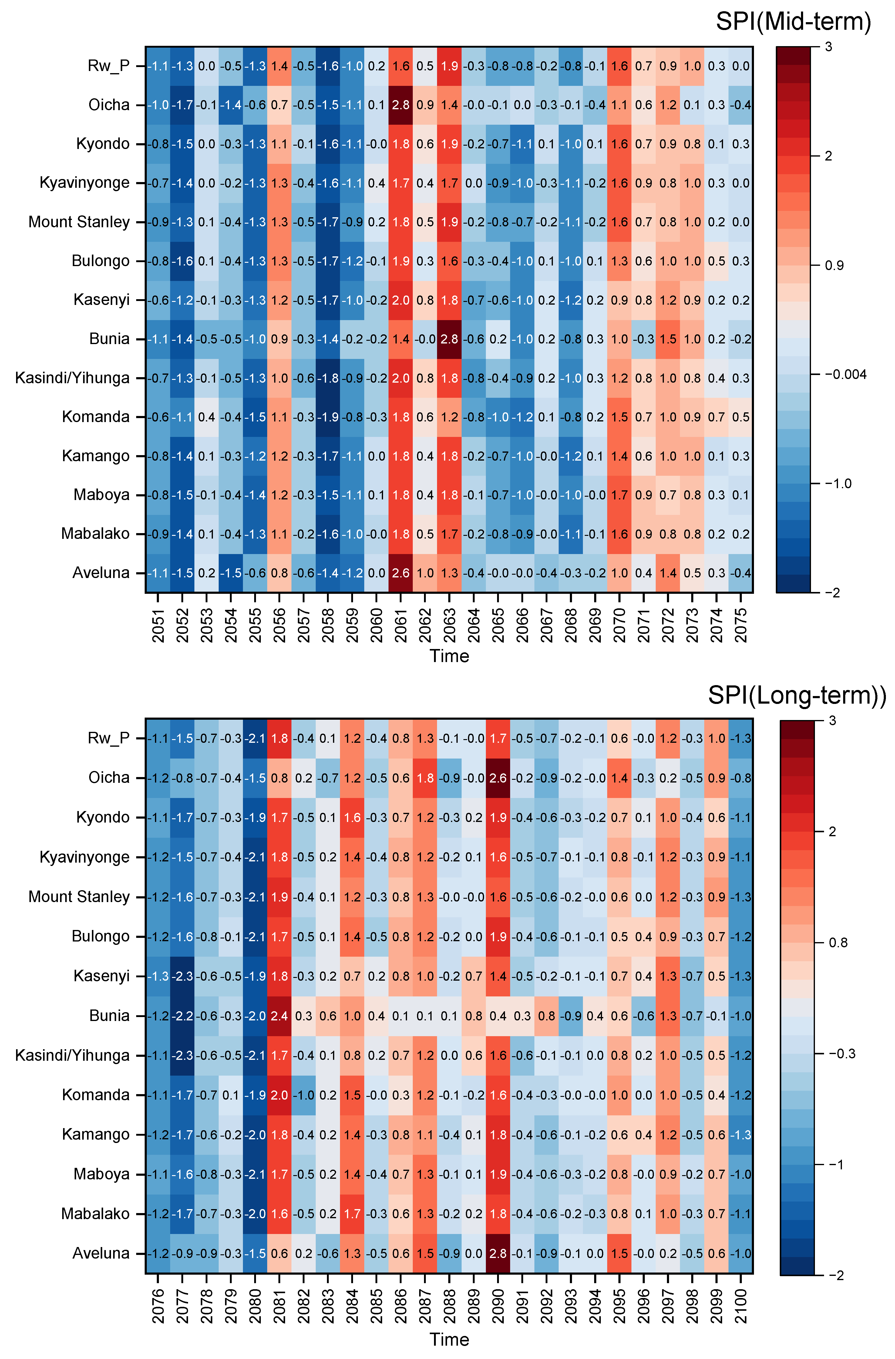
3.5. SPI Analysis of Historical and Future Drought Trends

Analyzing the drought trends using the standardized precipitation index (SPI) for the Beni–Irumu region, it is observed that the severity of drought varies from year to year, with some areas experiencing more extreme conditions than others. Historical data analysis, as shown in Figure 9, indicates that severe and extremely dry conditions were notably observed in the years 1984, 1991, 2002, 2003, and 2009. During these years, regions such as Kasenyi, Bunia, Aveluna, Kyavinyonge, Oicha, Kasindi/Yihunga, and Mount Stanley were the most affected. In the near future, under the SSP5-8.5 scenario, severe dry conditions are expected for the years 2026, 2031, and 2046, with almost the entire region potentially affected by these severe dry conditions. Conversely, the year 2050 is expected to experience severely wet conditions.

For the mid-term period, as illustrated in Figure 10, the years 2052, 2055, and 2058 are projected to be the most affected by severe drought conditions, similar to the near-term period, where the entire region is likely to be impacted. Looking further into the long-term period, the years 2077 and 2080 are anticipated to be marked by severely dry conditions, affecting most areas of the Beni–Irumu region. This analysis highlights the significant variability in drought severity and the widespread impact of these conditions over time, emphasizing the need for adaptive strategies to mitigate the adverse effects on the region’s environment and socio-economic conditions.

4. Discussion

The analysis of annual rainfall patterns over different time scales in the Beni–Irumu region underscores the complex interplay of spatial and temporal variations. From historical as well as projected analyses, the region has exhibited distinct spatial disparities, with high-altitude areas receiving higher rainfall amounts compared to low-altitude locations (Figure 1 and Figure 3a). This pattern is attributed to orographic effects, highlighting the significant role of topography in rainfall distribution.

Orographic effects are particularly evident around Mount Stanley, one of the peaks of the Rwenzori Mountains. Here, the mountain acts as a prominent barrier forcing moisture-laden air from prevailing wind directions to rise and cool. The prevailing wind direction in the Beni–Irumu region is associated with an intensification of the trade winds towards East Africa, bringing water vapor from the Indian Ocean [39]. Additionally, regional water bodies and local evaporation processes significantly contribute to the water vapor in the region [40]. Furthermore, the Buganda–Toro belt’s influence on the western part of the East African Rift system impacts the water vapor dynamics in the Rwenzori Mountains, with the belt’s structure affecting rift propagation and fault development within the region [41]. This process enhances condensation and leads to increased rainfall [42,43]. As altitude increases, air parcels experience lower atmospheric pressure and temperature, resulting in their expansion and subsequent cooling. Cooler air holds less moisture, causing the condensation of water vapor and cloud formation, which eventually leads to rainfall [44]. This phenomenon explains the higher mean rainfall values in elevated regions like Mount Stanley and Kyondo compared to lower areas like Kasenyi, Bunia, Kyavinyonge, and Kasindi/Yihunga within the Semuliki River Basin, part of the Albertine Rift Valley [45].

The observed orographic effects in the Beni–Irumu region’s rainfall distribution are consistent with similar findings in other mountainous regions worldwide, such as the Himalayas, the German Alps [46,47,48], the Western Ghats in India, the Andes in South America, and the Cascade Range in the United States [49,50,51,52].

By overlaying Figure 2a,b onto Figure 1, we observe that the concentration and spatial distribution of precipitation in the southern part of the study area, corresponding to the equator line zone, are likely influenced not only by orographic effects but also by the Intertropical Convergence Zone (ITCZ) [53,54]. The ITCZ is a belt of low pressure that encircles the Earth near the equator, where trade winds from the Northern and Southern Hemispheres converge. This convergence causes warm, moist air to rise, leading to the formation of thunderstorms and heavy rainfall. Consequently, regions within the ITCZ experience increased precipitation, while areas outside its influence may receive significantly less rainfall [55]. This dual influence of orography and the ITCZ results in a highly variable rainfall distribution, with some areas experiencing heavy, consistent rainfall and others facing drier conditions.

In addition to orographic effects, which play a significant role in shaping precipitation patterns, the observed low precipitation values in the Kasenyi and Kyavinyonge areas can also be attributed to their proximity to water bodies such as Lake Albert and Lake Edward, respectively. This observation aligns with findings from studies conducted in the United States, where lakeshore areas often exhibit reduced precipitation compared to their surrounding regions due to various factors. Recent research focusing on changes in precipitation patterns across the Great Lakes and Midwest has highlighted increased rates and totals, with notable spatial variability in trends [56]. Moreover, the phenomenon of lake-effect precipitation, prevalent over the Great Lakes region, offers valuable insights into how proximity to large water bodies can influence local weather conditions. When cold air masses pass over warm lake waters, particularly under specific wind conditions, the result is locally higher rainfall amounts, a process documented in studies such as that by [57]. Furthermore, the interaction between lake surface temperature and the atmosphere plays a pivotal role in shaping regional climate dynamics. Ref. [58] underscored this point in their research, highlighting how variations in lake surface temperature can impact convective environments and precipitation processes over the Great Lakes Region.

Given the broader context of the Albertine Rift Valley region, it is crucial to consider not only Lakes Albert and Edward but also other significant water bodies such as Lakes Kivu and Tanganyika. The presence of multiple lakes within the same geographical area necessitates a comprehensive study to fully understand their collective impacts on the spatial distribution of climate. This study would need to explore the complex interactions between these lakes and surrounding atmospheric conditions, including their influence on local weather patterns, precipitation regimes, and broader climatic dynamics.

Under the hypothesis of concentrations of greenhouse gases that lead to an increase in radiative forcing by 8.5 watts per square meter by the year 2100, often considered a “worst-case” scenario (SSP5-8.5 scenario) [59], the projected variations in rainfall patterns across the Beni–Irumu region carry significant implications for local communities and ecosystems. In the near term, areas experiencing substantial reductions in rainfall, such as Oicha, are likely to face heightened risks of water scarcity, crop failures, and ecosystem degradation, while regions like Kasindi/Yihunga, with relatively stable rainfall projections (Figure 7a), may still face climate-related challenges, albeit to a lesser extent. However, the mid-term (Figure 7b) outlook presents a mixed picture, with some areas showing signs of rainfall recovery. This may offer temporary relief, but persistent challenges in locations like Oicha underscore the need for proactive adaptation measures such as water conservation, crop diversification, and sustainable land management practices. In the long term (Figure 7c), overall improvements in rainfall projections offer hope for enhanced climate resilience, yet persistent disparities in vulnerable areas like Oicha highlight the need for targeted interventions and long-term planning. Increased rainfall in Kasindi/Yihunga, Bulongo, and Kyavinyonge may initially seem beneficial, but it is crucial to consider potential long-term issues such as water management, infrastructure, flooding, soil erosion, and landslides, which can threaten human settlements, agriculture, and local economies. Investing in climate-resilient infrastructure, early warning systems, and community-based adaptation strategies is crucial to addressing the multifaceted challenges posed by changing rainfall patterns [60,61].

These worst anticipated trends in rainfall for various areas in the Beni–Irumu region, under a high greenhouse gas emissions scenario, emphasizes the necessity of incorporating additional scenarios into current modeling approaches for a more comprehensive assessment. Future studies should incorporate scenarios characterized by lower and moderate greenhouse gas emissions and environmental impacts, such as SSP1-1.9, SSP1-2.6, SSP5-3.4OS, and SSP2-4.5 [62,63].

The observed decreasing trend in rainfall during the near-term period (2026–2050) compared to the historical period (1983–2016), followed by an increasing trend in the mid-term (2051–2075) and far-term (2076–2100) periods, under the SSP5-8.5 scenario can be attributed to complex feedback mechanisms simulated by climate models. In the context of the Beni–Irumu region in the eastern region of the Democratic Republic of Congo (DRC), changes in the position and intensity of the Intertropical Convergence Zone (ITCZ) play a significant role in driving seasonal rainfall patterns. During the near-term period, shifts in atmospheric circulation patterns and variations in sea surface temperatures can lead to reduced rainfall as the ITCZ moves away from the region or weakens. This reduction is followed by a gradual recovery and increase in rainfall in the mid-term and far-term periods, potentially due to the strengthening of the ITCZ or changes in regional climate dynamics that enhance moisture availability. These variations in rainfall are consistent with the broader understanding of how climate models simulate the impact of global climate phenomena, such as the Indian Ocean Dipole (IOD) and El Niño Southern Oscillation (ENSO), on regional precipitation patterns [64,65,66].

5. Conclusions

The study provides valuable insights into the spatial and temporal variations in rainfall distribution in the Beni–Irumu region by using CHIRPS data and climate models. The results demonstrate the effectiveness of the Ensemble model in simulating rainfall patterns and reveal significant disparities influenced by topography and climate change. Historical data show notable spatial disparities, with high-altitude areas like Mount Stanley receiving significantly more rainfall compared to low-altitude regions like Kasenyi. Future projections under the SSP5-8.5 scenario indicate substantial decreases in rainfall for areas like Oicha, while regions like Kasindi/Yihunga may maintain relatively stable levels. In the near future, a remarkable decrease in rainfall is expected across almost all areas. Mid-term projections show signs of recovery in some areas, but long-term projections suggest overall improvements in rainfall, albeit with persistent disparities in the Oicha region. These findings underscore the necessity for targeted interventions and adaptive strategies to address the varied impacts of climate change on rainfall distribution, particularly in vulnerable regions like Oicha. This will enable informed decision-making for enhancing climate resilience and supporting sustainable development in the Beni–Irumu region.

References

1. Intergovernmental Panel on Climate Change (IPCC). Climate Change 2021—The Physical Science Basis: Contribution of Working Group I to the Sixth Assessment Report of the Intergovernmental Panel on Climate Change; Cambridge University Press: Cambridge, UK, 2021; Volume 2. [Google Scholar]
2. Banholzer, S.; Kossin, J.; Donner, S. The impact of climate change on natural disasters. In Reducing Disaster: Early Warning Systems for Climate Change; Springer: Dordrecht, The Netherlands, 2014; pp. 21–49. [Google Scholar] [CrossRef]
3. Kumar, N.; Poonia, V.; Gupta, B.B.; Goyal, M.K. A novel framework for risk assessment and resilience of critical infrastructure towards climate change. Technological 2021, 165, 120532. [Google Scholar] [CrossRef]
4. Javadinejad, S.; Dara, R.; Jafary, F. Analysis and prioritization the effective factors on increasing farmers resilience under climate change and drought. Agric. Res. 2021, 10, 497–513. [Google Scholar] [CrossRef]
5. Alahacoon, N.; Edirisinghe, M. Spatial variability of rainfall trends in Sri Lanka from 1989 to 2019 as an indication of climate change. ISPRS Int. J. Geo-Inf. 2021, 10, 84. [Google Scholar] [CrossRef]
6. Abtew, W.; Dessu, S.B.; Abtew, W.; Dessu, S.B. Grand Ethiopian renaissance dam analysis. In The Grand Ethiopian Renaissance Dam on the Blue Nile; Springer: Cham, Switzerland, 2019; pp. 79–96. [Google Scholar] [CrossRef]
7. Kapiri, M.M.; Mahamba, J.A.; Amani, R.K.; Mulondi, G.K.; Sahani, W.M. Drought from the 1970s to the 1990s and its Influence in the Tropical City of Beni, Eastern DR Congo. Indones. J. Soc. Environ. Issues 2023, 4, 45–58. [Google Scholar] [CrossRef]
8. Posite, V.R.; Ahana, B.S.; Abdelbaki, C.; Zerga, A.; and Guadie, A. Analysis of temperature and rainfall trends in Beni City, Democratic Republic of Congo. J. Earth Syst. Sci. 2024, 133, 102. [Google Scholar] [CrossRef]
9. Gebrechorkos, S.H.; Hülsmann, S.; Bernhofer, C. Long-term trends in rainfall and temperature using high-resolution climate datasets in East Africa. Sci. Rep. 2019, 9, 11376. [Google Scholar] [CrossRef] [PubMed]
10. Banerjee, A.; Chen, R.E.; Meadows, M.; Singh, R.B.; Mal, S.; Sengupta, D. An analysis of long-term rainfall trends and variability in the uttarakhand himalaya using google earth engine. Remote Sens. 2020, 12, 709. [Google Scholar] [CrossRef]
11. Paredes-Trejo, F.J.; Barbosa, H.A.; Kumar, T.L. Validating CHIRPS-based satellite precipitation estimates in Northeast Brazil. J. Arid Environ. 2017, 139, 26–40. [Google Scholar] [CrossRef]
12. Nkunzimana, A.; Bi, S.; Alriah, M.A.A.; Zhi, T.; Kur, N.A.D. Comparative analysis of the performance of satellite-based rainfall products over various topographical unities in Central East Africa: Case of Burundi. Earth Space Sci. 2020, 7, e2019EA000834. [Google Scholar] [CrossRef]
13. Dinku, T.; Funk, C.; Peterson, P.; Maidment, R.; Tadesse, T.; Gadain, H.; Ceccato, P. Validation of the CHIRPS satellite rainfall estimates over eastern Africa. Q. J. R. Meteorol. Soc. 2018, 144, 292–312. [Google Scholar] [CrossRef]
14. Macharia, J.M.; Ngetich, F.K.; Shisanya, C.A. Comparison of satellite remote sensing derived precipitation estimates and observed data in Kenya. Agric. For. Meteorol. 2020, 284, 107875. [Google Scholar] [CrossRef]
15. Ngoma, H.; Wen, W.; Ojara, M.; Ayugi, B. Assessing current and future spatiotemporal precipitation variability and trends over Uganda, East Africa, based on CHIRPS and regional climate model datasets. Meteorol. Atmos. Phys. 2021, 133, 823–843. [Google Scholar] [CrossRef]
16. Mulungu, D.M.; Mukama, E. Evaluation and modelling of accuracy of satellite-based CHIRPS rainfall data in Ruvu subbasin, Tanzania. Model. Earth Syst. Environ. 2023, 9, 1287–1300. [Google Scholar] [CrossRef]
17. Getachew, B.; Manjunatha, B.R. Potential climate change impact assessment on the hydrology of the Lake Tana Basin, Upper Blue Nile River Basin, Ethiopia. Phys. Chem. Earth Parts A/B/C 2022, 127, 103162. [Google Scholar] [CrossRef]
18. Isinkaralar, O. Bioclimatic comfort in urban planning and modeling spatial change during 2020–2100 according to climate change scenarios in Kocaeli, Türkiye. Int. J. Environ. Sci. Technol. 2023, 20, 7775–7786. [Google Scholar] [CrossRef]
19. Ahmadalipour, A.; Rana, A.; Moradkhani, H.; Sharma, A. Multicriteria evaluation of CMIP5 GCMs for climate change impact analysis. Theor. Appl. Clim. 2017, 128, 71–87. [Google Scholar] [CrossRef]
20. Alaminie, A.A.; Tilahun, S.A.; Legesse, S.A.; Zimale, F.A.; Tarkegn, G.B.; Jury, M.R. Evaluation of Past and Future Climate Trends under CMIP6 Scenarios for the UBNB (Abay), Ethiopia. Water 2021, 13, 2110. [Google Scholar] [CrossRef]
21. Hofer, S.; Lang, C.; Amory, C.; Kittel, C.; Delhasse, A.; Tedstone, A.; Fettweis, X. Greater Greenland Ice Sheet contribution to global sea level rise in CMIP6. Nat. Commun. 2020, 11, 6289. [Google Scholar] [CrossRef] [PubMed]
22. Kamruzzaman, M.; Shahid, S.; Islam, T.; Hwang, S.; Cho, J.; Zaman, A.U.; Ahmed, M.; Rahman, M.; Hossain, B. Comparison of CMIP6 and CMIP5 model performance in simulating historical precipitation and temperature in Bangladesh: A preliminary study. Theor. Appl. Climatol. 2021, 145, 1385–1406. [Google Scholar] [CrossRef]
23. Song, Y.H.; Chung, E.S.; Shahid, S. Spatiotemporal differences and uncertainties in projections of precipitation and temperature in South Korea from CMIP6 and CMIP5 general circulation models. Int. J. Climatol. 2021, 41, 5899–5919. [Google Scholar] [CrossRef]
24. Wyser, K.; Kjellström, E.; Koenigk, T.; Martins, H.; Döscher, R. Warmer climate projections in EC-Earth3-Veg: The role of changes in the greenhouse gas concentrations from CMIP5 to CMIP6. Environ. Res. Lett. 2020, 15, 054020. [Google Scholar] [CrossRef]
25. Pu, Y.; Liu, H.; Yan, R.; Yang, H.; Xia, K.; Li, Y.; Dong, L.; Li, L.; Wang, H.; Nie, Y.; et al. CAS FGOALS-g3 model datasets for the CMIP6 scenario model intercomparison project (ScenarioMIP). Adv. Atmos. Sci. 2020, 37, 1081–1092. [Google Scholar] [CrossRef]
26. Yokoi, R.; Watari, T.; Motoshita, M. Future greenhouse gas emissions from metal production: Gaps and opportunities towards climate goals. Energy Environ. Sci. 2022, 15, 146–157. [Google Scholar] [CrossRef]
27. Estoque, R.C.; Ooba, M.; Togawa, T.; Hijioka, Y. Projected land-use changes in the Shared Socioeconomic Pathways: Insights and implications. Ambio 2020, 49, 1972–1981. [Google Scholar] [CrossRef]
28. Funk, C.; Peterson, P.; Landsfeld, M.; Pedreros, D.; Verdin, J.; Shukla, S.; Michaelsen, J. The climate hazards infrared precipitation with stations a new environmental record for monitoring extremes. Sci. Data 2015, 2, 1–21. [Google Scholar] [CrossRef]
29. Novella, N.S.; Thiaw, W.M. African rainfall climatology version 2 for famine early warning systems. J. Appl. Meteorol. Climatol. 2013, 52, 588–606. [Google Scholar] [CrossRef]
30. Krasting, J.P.; John, J.G.; Blanton, C.; McHugh, C.; Nikonov, S.; Radhakrishnan, A.; Rand, K.; Zadeh, N.T.; Balaji, V. NOAA-GFDL GFDL-ESM4 model output prepared for CMIP6 CMIP. Version YYYYMMDD. Earth Syst. Grid Fed. 2018. [Google Scholar] [CrossRef]
31. Volodin, E.; Mortikov, E.; Gritsun, A.; Lykossov, V.; Galin, V.; Diansky, N.; Gusev, A.; Kostrykin, S.; Iakovlev, N.; Shestakova, A.; et al. INM INM-CM5-0 model output prepared for CMIP6 CMIP piControl. Version YYYYMMDD. Earth Syst. Grid Fed. 2019. [Google Scholar] [CrossRef]
32. Themeßl, M.J.; Gobiet, A.; Heinrich, G. Empirical-statistical downscaling and error correction of regional climate models and its impact on the climate change signal. Clim. Chang. 2012, 112, 449–468. [Google Scholar] [CrossRef]
33. Hodson, T.O. Root-mean-square error (RMSE) or mean absolute error (MAE): When to use them or not. Geosci. Model Dev. 2022, 15, 5481–5487. [Google Scholar] [CrossRef]
34. Thao, S.; Garvik, M.; Mariethoz, G.; Vrac, M. Combining global climate models using graph cuts. Clim. Dyn. 2022, 59, 2345–2361. [Google Scholar] [CrossRef] [PubMed]
35. Zakeri, S.; Samkhaniani, A.; Adeli, S.; Nikraftar, Z. Evaluation of long-term trend of different drought indices using Mann-Kendall and Sen’s slope estimator over Iran. Int. Arch. Photogramm. Remote Sens. Spat. Inf. Sci. 2019, 42, 1141–1145. [Google Scholar] [CrossRef]
36. Nyikadzino, B.; Chitakira, M.; Muchuru, S. Rainfall and runoff trend analysis in the Limpopo River basin using the Mann-Kendall statistic. Phys. Chem. Earth Parts A/B/C 2020, 117, 102870. [Google Scholar] [CrossRef]
37. Salarian, M.; Larijani, S.; Banejad, H.; Heydari, M.; Ghadim, H.B. Trend analysis of water flow on Neka and Tajan rivers using parametric and non-parametric tests. Időjárás/Q. J. Hung. Meteorol. Serv. 2022, 126, 387–402. [Google Scholar] [CrossRef]
38. McKee, T.B.; Doesken, N.J.; Kleist, J. The relationship of drought frequency and duration to time scales. In Proceedings of the 8th Conference on Applied Climatology, Anaheim, CA, USA, 17–22 January 1993; Volume 17, pp. 179–183. [Google Scholar]
39. Beltrando, G. Variabilité Interannuelle des Précipitations en Afrique Orientale (Kenya, Ouganda, Tanzanie) et Relations Avec la Dynamique de l’Atmosphère. Ph.D. Thesis, University of the Mediterranean, Marseille, France, 1990. [Google Scholar]
40. Mansour, S.; Bauer, F.; Glasmacher, U.; Grobe, R.; Starz, M. Thermo-tectonic history reconstruction of the Rwenzori Mountains, Geophys. Res. Abstr. 2014, 17. [Google Scholar]
41. Koehn, D.; Link, K.; Sachau, T.; Passchier, C.W.; Aanyu, K.; Spikings, A.; Harbinson, R. The Rwenzori Mountains, a Palaeoproterozoic crustal shear belt crossing the Albertine rift system. Int. J. Earth Sci. 2016, 105, 1693–1705. [Google Scholar] [CrossRef]
42. Dettinger, M.D.; Lavers, D.A.; Compo, G.P.; Gorodetskaya, I.V.; Neff, W.; Neiman, P.J.; Ramos, A.M.; Rutz, J.J.; Viale, M.; Wade, A.J.; et al. Effects of Atmospheric Rivers. In Atmospheric Rivers; Springer: Cham, Switzerland, 2020; pp. 141–177. [Google Scholar] [CrossRef]
43. Vimont, U.; Gain, J.; Lastic, M.; Cordonnier, G.; Abiodun, B.; Cani, M.P. Interactive Meso-scale Simulation of Skyscapes. Comput. Graph. Forum 2020, 39, 585–596. [Google Scholar] [CrossRef]
44. Linke, M.; Praeger, U.; Neuwald, D.A.; Geyer, M. Measurement of Water Vapor Condensation on Apple Surfaces during Controlled Atmosphere Storage. Sensors 2023, 23, 1739. [Google Scholar] [CrossRef]
45. Tumushabe, M.W.; Helland-Hansen, W.; Nagudi, B.; Echegu, S.; Aanyu, K. Quantification of reservoir rock properties (Porosity, Permeability and Vshale) in the reservoir rock units of South Lake Albert Basin, Albertine Rift, Western Uganda. J. Afr. Earth Sci. 2022, 185, 104410. [Google Scholar] [CrossRef]
46. Ademe, D.; Zaitchik, B.F.; Tesfaye, K.; Simane, B.; Alemayehu, G.; Adgo, E. Climate trends and variability at adaptation scale: Patterns and perceptions in an agricultural region of the Ethiopian Highlands. Weather Clim. Extrem. 2020, 29, 100263. [Google Scholar] [CrossRef]
47. Yadav, J.S.; Tiwari, S.K.; Misra, A.; Rai, S.K.; Yadav, R.K. High-altitude meteorology of Indian Himalayan Region: Complexities, effects, and resolutions. Environ. Monit. Assess. 2021, 193, 654. [Google Scholar] [CrossRef] [PubMed]
48. Fujinami, H.; Fujita, K.; Takahashi, N.; Sato, T.; Kanamori, H.; Sunako, S.; Kayastha, R.B. Twice-daily monsoon precipitation maxima in the Himalayas driven by land surface effects. J. Geophys. Res. Atmos. 2021, 126, e2020JD034255. [Google Scholar] [CrossRef]
49. Saranya, P.; Krishnakumar, A.; Sinha, N.; Kumar, S.; Krishnan, K.A. Isotopic signatures of moisture recycling and evaporation processes along the Western Ghats orography. Atmos. Res. 2021, 264, 105863. [Google Scholar] [CrossRef]
50. Shen, H.; Lynch, B.; Poulsen, C.J.; Yanites, B.J. A modeling framework (WRF-Landlab) for simulating orogen-scale climate-erosion coupling. Comput. Geosci. 2021, 146, 104625. [Google Scholar] [CrossRef]
51. Padmakumari, B.; Kalgutkar, S.; Sunil, S.; Nikam, M.; Pandithurai, G. High temporal variability of surface solar irradiance due to cloud enhancement effect over the Western Ghat mountains in peninsular India. J. Atmos. Sol. Terr. Phys. 2022, 232, 105867. [Google Scholar] [CrossRef]
52. He, J.; Yang, R.; Su, C. Data-based analysis about the influence on erosion rates of the Tibetan Plateau. J. Asian Earth Sci. 2022, 233, 105246. [Google Scholar] [CrossRef]
53. Miah, M.A. The ONR-602 Experiment and investigation of particle precipitation near the equator. J. Geomagn. Geoelectr. 1991, 43, 445–460. [Google Scholar] [CrossRef]
54. Mackay, A.W.; Lee, R.; Russell, J.M. Recent climate-driven ecological changes in tropical montane lakes of Rwenzori Mountains National Park, central Africa. J. Paleolimnol. 2021, 65, 219–234. [Google Scholar] [CrossRef]
55. Jung, H.; Knippertz, P.; Ruckstuhl, Y.; Redl, R.; Janjic, T.; Hoose, C. Understanding the dependence of mean precipitation on convective treatment in tropical aquachannel experiments. Weather. Clim. Dyn. Discuss. 2023, 4, 1111–1134. [Google Scholar] [CrossRef]
56. Zhang, X.; Wang, H.; Li, Z.; Xie, J.; Ni, J. Hydrological and soil physiochemical variables determine the rhizospheric microbiota in subtropical lakeshore areas. PeerJ 2020, 8, e10078. [Google Scholar] [CrossRef] [PubMed]
57. Pakzad, S.; Keshtkar, A.R.; Keshtkar, H.; Atashi, H.; Afzali, A. Impact of lake surface changes on climate fluctuation within a lake-affected region. Environ. Earth Sci. 2021, 80, 160. [Google Scholar] [CrossRef]
58. Baule, W.J.; Andresen, J.A.; Winkler, J.A. Trends in Quality Controlled Precipitation Indicators in the United States Midwest and Great Lakes Region. Front. Water 2022, 4, 817342. [Google Scholar] [CrossRef]
59. Pachauri, R.K.; Allen, M.R.; Barros, V.R.; Broome, J.; Cramer, W.; Christ, R.; Church, J.A.; Clarke, L.; Dahe, Q.D.; Dasqupta, P.; et al. Climate Change 2014—Synthesis Report: Contribution of Working Groups I, II and III to the Fifth Assessment Report of the Intergovernmental Panel on Climate Change; IPCC: Geneva, Switzerland, 2014; p. 151. [Google Scholar]
60. Chacowry, A. Meeting the challenges to climate change adaptation: An NGO community-based successful projects in Mauritius. GeoJournal 2023, 88, 4081–4094. [Google Scholar] [CrossRef] [PubMed]
61. Buhl, M.; Markolf, S. A review of emerging strategies for incorporating climate change considerations into infrastructure planning, design, and decision making. Sustain. Resilient Infrastruct. 2023, 8 (Suppl. 1), 157–169. [Google Scholar] [CrossRef]
62. Riahi, K.; Van Vuuren, D.P.; Kriegler, E.; Edmonds, J.; O’neill, B.C.; Fujimori, S.; Bauer, N.; Calvin, K.; Dellink, R.; Fricko, O.; et al. The Shared Socioeconomic Pathways and their energy, land use, and greenhouse gas emissions implications: An overview. Glob. Environ. Chang. 2017, 42, 153–168. [Google Scholar] [CrossRef]
63. O’Neill, B.C.; Kriegler, E.; Ebi, K.L.; Kemp-Benedict, E.; Riahi, K.; Rothman, D.S.; van Ruijven, B.J.; van Vuuren, D.P.; Birkmann, J.; Kok, K.; et al. The roads ahead: Narratives for shared socioeconomic pathways describing world futures in the 21st century. Glob. Environ. Chang. 2017; 42, 169–180. [Google Scholar]
64. Hulme, M.; Doherty, R.; Ngara, T.; New, M.; Lister, D. African climate change: 1900–2100. Clim. Res. 2001, 17, 145–168. [Google Scholar] [CrossRef]
65. Nicholson, S.E. Climate and climatic variability of rainfall over eastern Africa. Rev. Geophys. 2017, 55, 590–635. [Google Scholar] [CrossRef]
66. Washington, R.; Harrison, M.; Conway, D. African climate change: Taking the shorter route. Bull. Am. Meteorol. Soc. 2006, 87, 1355–1366. [Google Scholar] [CrossRef]
Figure 1. Beni–Irumu region’s location map.
Remotesensing 16 02819 g001
Figure 2. Ensemble model performance. Observed (a); Simulated (b).
Remotesensing 16 02819 g002
Figure 3. Spatial rainfall distribution for historical (a), near-term (b), mid-term (c), and long-term (d) time scales.
Remotesensing 16 02819 g003
Figure 4. Rainfall distribution across virtual weather stations for historical (a), near-term (b), mid-term (c), and long-term (d) time scales.
Remotesensing 16 02819 g004
Figure 5. Monthly rainfall distribution for historical (1983–2014) and near-term (2026–2050) periods. (a): Depicts the monthly rainfall distribution over the historical period, illustrating long-term precipitation patterns. (b): Shows the monthly rainfall distribution for near-term period, highlighting recent trends and potential changes in precipitation.
Remotesensing 16 02819 g005
Figure 6. Monthly rainfall distribution for mid-term (2051–2075) and long-term (2076–2100) periods. (a): Depicts the monthly rainfall distribution over the mid-term period, illustrating long-term precipitation patterns. (b): Shows the monthly rainfall distribution for long-term period, highlighting recent trends and potential changes in precipitation.
Remotesensing 16 02819 g006
Figure 7. Difference between near-term and historical rainfall (a); Difference between mid-term and historical rainfall (b); Difference between long-term and historical rainfall (c).
Remotesensing 16 02819 g007
Figure 8. Rainfall trend analysis in Beni–Irumu region. “*” indicates stations showing significant trends.
Remotesensing 16 02819 g008
Figure 9. Historical and near-term SPI analysis.
Remotesensing 16 02819 g009
Figure 10. Mid-term and long-term SPI projections.
Remotesensing 16 02819 g010