Abstract
Effective forest management is essential for mitigating climate change effects. This is why understanding forest growth dynamics is critical for its sustainable management. Thus, characterizing forest plot deadwood levels is vital for understanding forest dynamics, and for assessments of biomass, carbon stock, and biodiversity. For the first time, this study used the leaf area index (LAI) and L-moments to characterize and model forest plot deadwood levels in the Bavarian Forest National Park from airborne laser scanning (ALS) data. This study proposes methods that can be tested for forests, especially those in temperate climates with frequent cloud coverage and limited access. The proposed method is practically significant for effective planning and management of forest resources. First, plot decay levels were characterized based on their canopy leaf area density (LAD). Then, the deadwood levels were modeled to assess the relationships between the vegetation area index (VAI), gap fraction (GF), and the third L-moment ratio (T3). Finally, we tested the rule-based methods for classifying plot decay levels based on their biophysical structures. Our results per the LAD vertical profiles clearly showed the declining levels of decay from Level 1 to 5. Our findings from the models indicate that at a 95% confidence interval, 96% of the variation in GF was explained by the VAI with a significant negative association (VAIslope = −0.047; R2 = 0.96; (p < 0.001)), while the VAI explained 92% of the variation in T3 with a significant negative association (VAIslope = −0.50; R2 = 0.92; (p < 0.001)). Testing the rule-based methods, we found that the first rule (Lcv = 0.5) classified Levels 1 and 2 at (Lcv < 0.5) against Levels 3 to 5 at (Lcv > 0.5). However, the second rule (Lskew = 0) classified Level 1 (healthy plots) as closed canopy areas (Lskew < 0) against Levels 2 to 5 (deadwood) as open canopy areas (Lskew > 0). This approach is simple and more convenient for forest managers to exploit for mapping large forest gap areas for planning and managing forest resources for improved and effective forest management.
1. Introduction
Forests are a fundamental section of natural ecosystems that all living organisms depend on. Consequently, its management and maintenance are critical for living organisms’ survival and the environment at large. Especially in the era of global warming, winning the battle against climate change is most likely to be impossible without healthy forest ecosystems. Thus, understanding the declining state of the forest is very important to be able to revive its growth through appropriate management. This is why characterizing and evaluating forest decay levels and deadwood is important for understanding forest growth dynamics, and for assessing biomass, carbon storage, and biodiversity.
The Bavarian Forest National Park (BFNP), in Germany, is a natural temperate forest dominated by conifer species, especially the Norway spruce (more details about this forest are given in Section 2.1). This forest has been disturbed over the years by windthrow and bark beetle (Ips typographus) insect infestations [1,2]. This disturbance decline [3,4] resulted in the death of old trees, which further declined (decay levels) from their death to snags. Trees after their death go through successional decomposition stages from defoliation, twig, and branch reduction to snags and total collapse at a very slow rate [3]. Early studies in the 1970s and before qualitatively characterize tree decomposition stages and dynamics [3,4]. Thomas [4], for instance, displayed a visual conceptual classification of decay stages from a healthy tree to a stump in nine stages. Most of these characterizations in the past used the traditional approach for assessing and characterizing forest decay levels and deadwood, which is normally through field measurements and assessments. However, aside from its labor intensiveness and time-consuming factor, forest field measurement comes with several difficulties and challenges including the risk of accidents, despite its effectiveness, especially at the single tree level. This, coupled with the lack of access to some parts of the forest due to obstacles (e.g., flood) or the undulating nature of the terrain, makes it inconvenient and unsustainable, especially for larger forest areas. Thus, characterizing and estimating the decay levels using a cost-effective approach are needed for improved and sustainable forest management.
Thankfully, advancement in remote sensing technologies has brought some relief to the traditional approach of forest mensuration and management leveraging time and cost. This further comes with mapping larger areas without necessarily needing physical presence in the forest [5]. For the past decades, researchers have extensively used passive and active sensors as well as a combination of both for monitoring and tracking forest health and growth dynamics toward its effective management [6,7,8,9,10,11]. While other sensors capture only a 2D view (imagery) of forests, Light Detection and Ranging (LiDAR) [12,13,14] can capture the 3D structural view of forests with higher resolution and accuracy, making it indispensable for forestry applications. LiDAR has a scanning mechanism for emitting pulses of laser light with a wavelength in the near infrared (NIR) range from a platform (mostly either via airborne laser scanning (ALS), unmanned aerial vehicles (UAV), or terrestrial laser scanning (TLS)) to targeted trees in the forest [12]. These pulses, after hitting the forest, return pulse signals in the form of continuous waves (full-waveform) [15] or discrete returns [16] corresponding to the forest structure in the form of 3D point clouds. Furthermore, contrary to other sensors, LiDAR’s ability to penetrate through spaces in tree canopies and forest gaps makes it extraordinarily special for forest mensuration and assessments, as it captures the sub-canopy and topography as well [17].
Another challenge in forest research is the need for field data for the validation of remote sensing data. However, it is equally important to acknowledge the circumstances where acquiring field data could be impossible, especially in natural forests, due to several factors and obstacles that render parts of the forest physically inaccessible. Notwithstanding, data could be acquired through remote sensing. In such situations, forest remote sensing experts can assist with their field experience to visually interpret remote sensing data for research to prevail using sound-tested techniques without field data. LiDAR point cloud attributes and metrics have been proven to describe forest structure better and independently in 3D. The significance of LiDAR metrics in forest structural estimation and analysis has been reported [18,19,20,21]. Thus, the strength of LiDAR can be relied upon for characterizing forest plot decay levels without field data, although it is always good to have a ground reference.
The subject of tree decomposition using remote sensing technologies, despite its great importance to forest managers in the assessment of biodiversity, carbon storage/sequestration, and forest health in general, has so far received very little attention. Recently, in their assessment of habitat quality using multispectral imagery (Worldview-2 with panchromatic and 8 bands), Soto et al. [22] reported the relationship between the plant senescence reflectance index (PSRI) and wood decay stages resulting from woodpeckers with pixel-based image analysis. Putman et al. [23] studied the changes in standing dead trees (SDTs) at various decay levels over time based on volume estimates using multi-temporal TLS data. In a related study more recently, Klockow et al. [24] also studied the structural changes in SDT at different decay stages based on an allometric relationship of volume estimates and confirmed the efficiency of using TLS data for such a task. While these recent studies reaffirm the necessity of considering both the horizontal and vertical dimensions of trees in estimating and assessing forest decomposition, the consideration of LAI/LAD and gap fraction (GF) in assessing forest decomposition has received little or no attention. Researchers have defined LAI as the hemispherical surface area of a leaf per unit of the ground area [25,26], while LAD was defined as the per unit volume of the total amount of leaf area [27]. Thus, LAI can be derived from the LAD vertical profile [28,29]. Generally, while canopy GF serves as a variant for calculating LAI [30,31,32], the LAI/LAD has been used to quantify and estimate canopy volume and its vertical structure from varied remote sensors in direct and indirect approaches [27,30,33,34,35]. However, to the best of our knowledge, there has not been any work that considered the LAI/LAD approach in characterizing and estimating forest plot decay levels, which this study seeks to achieve.
In this study, we hypothesize that trees at various decay levels biophysically change in size and structure, which are often due to defoliation, twigs/branch reduction, and/or shrinkage. This change in size and structure describes the pattern of forest plots according to their decay levels and determines the amount of light intensity that can reach sub-canopies within the forest area. Consequently, in contrast to the optical sensors, ALS [19,36,37,38] has the potential to estimate forest canopy attributes and derive tree biophysical parameters such as LAI/LAD and GF with higher accuracy [17,39]. We equally hypothesize that the L-moments (Section 2.6) are equally significant in estimating and characterizing forest plot decay levels from ALS height returns without field data. Thus, in estimating and characterizing five forest plot decay levels (Levels 1 to 5), we evaluate the mutual relationship between the L-moment ratio, LAI/LAD, and its properties (vegetation area index (VAI) and GF) from ALS data. Furthermore, we test the rule-based methods to assess how they classify our decay levels. Therefore, the objectives for the study are as follows:
- To characterize forest plots decay levels based on LAI/LAD vertical profile from ALS data.
- To mutually evaluate the relationships between VAI, GF, and L-moment ratios on the decay levels.
- To characterize and model the decay levels based on the relationships between the VAI, GF, and L-moment ratios.
- To test the rule-based methods in classifying the forest plot decay levels.
2. Materials and Methods
2.1. Study Area
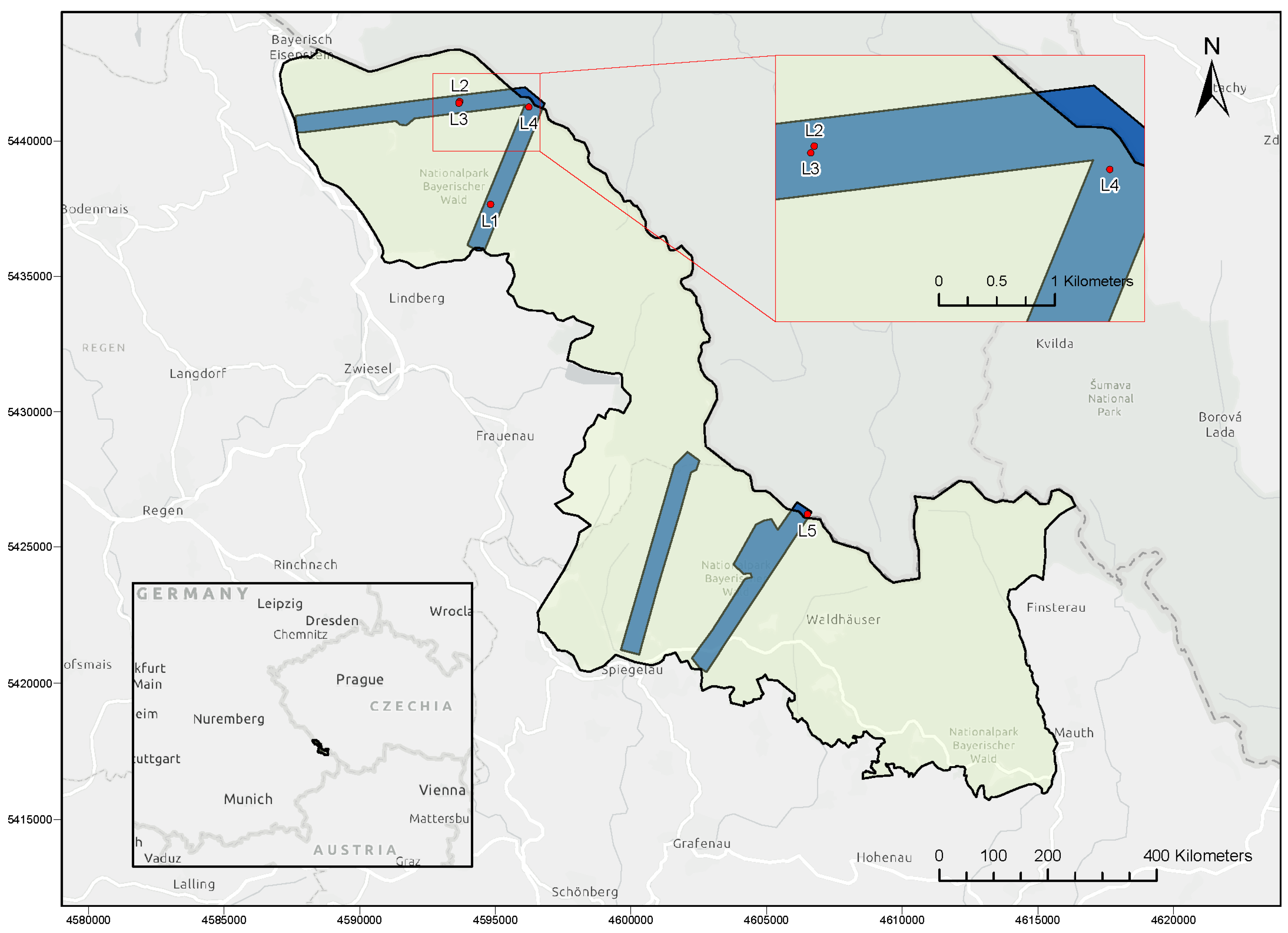
Our study area is in the BFNP (Figure 1), a 242.5 square km natural forest in the southeastern part of Germany that shares a boundary with the Czech Republic at 49.10 degrees north, and 13.22 degrees east. Being the oldest established park since the 1970s, the goal was to prevent human interference in the forest to enable the protection of its natural processes [2,40]. For this reason, although the forest witnessed strong thunderstorms in the 1980s and a subsequent bark beetle (Ips typographus) infestation in the 1990s [1], it had just about a 22% mortality rate by the year 2009 [41]. The conifer-dominated forest has a rough terrain with elevations between 600 and 1453 m, making it difficult to physically access some areas for field measurements, hence the need for remote sensing measurements and techniques like the ALS [2]. The Norway spruce (Picea abies) dominates the forest species followed by European beech (Fagus sylvatica), European silver fir (Abies alba), and other spruce species [42].
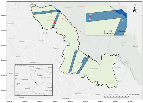
Figure 1.
Map of the BFNP (light green) illustrating regions of the three ALS transects (blue) and the selected plots (red).
2.2. Data Acquisition and Pre-Processing
The point cloud data used in this study were acquired on 18 August 2016, using a Riegl LMS-Q680i-400 kHz scanner (ALS) at an altitude of 300 m above sea level. These data were acquired in three transects in 1000 by 1000 m tiles, covering a 13.5 square km area of the BFNP with total raw points of 5.51 billion at a sampling rate of greater than 70 points per square meter. The flight was conducted by Milan Geoservice GmbH who pre-processed the raw data and corrected it with reference to the WGS84/UTM and transformed it to fit the Gauss–Kruger coordinate system (EPSG = 31468; DHDN 3-Degree Gauss zone 4). Then, it was finally formatted to LAZ 1.2. This data acquisition was part of the BFNP administration project for the Bohemian Forest Ecosystem [43,44]. The plots considered for this study were extracted from these data (Figure 1).
The color infrared (CIR) imagery used to support selecting plots of decay levels 1–5 (Figure 2) was acquired on 23 June 2016 using a DMC 122 camera onboard a Cessna 207 aircraft during a flight campaign over the entire BFNP at an average altitude of 2918 m above mean sea level [2,44]. With three spectral bands (near infrared, red, and green), the images were radiometrically corrected and orthorectified based on optimal camera calibration observations, transformation parameters, and ground control points. This was realized using the Trimble/INPHO company’s program system OrthoBox (Orthovista, Orthomaster). The ground resolution of the imagery was 20 cm.
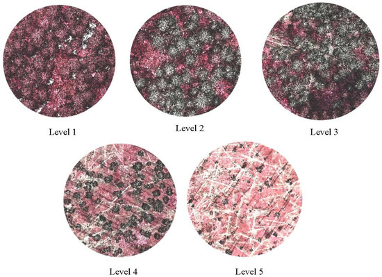
Figure 2.
The five selected plots (at 30 m radius) decay levels resulting from a fusion of the ALS point clouds and CIR imagery viewing from above the canopies. The healthy trees are reddish to brown while the dead trees are gray/dark gray to green in color.
2.3. Plot Selection
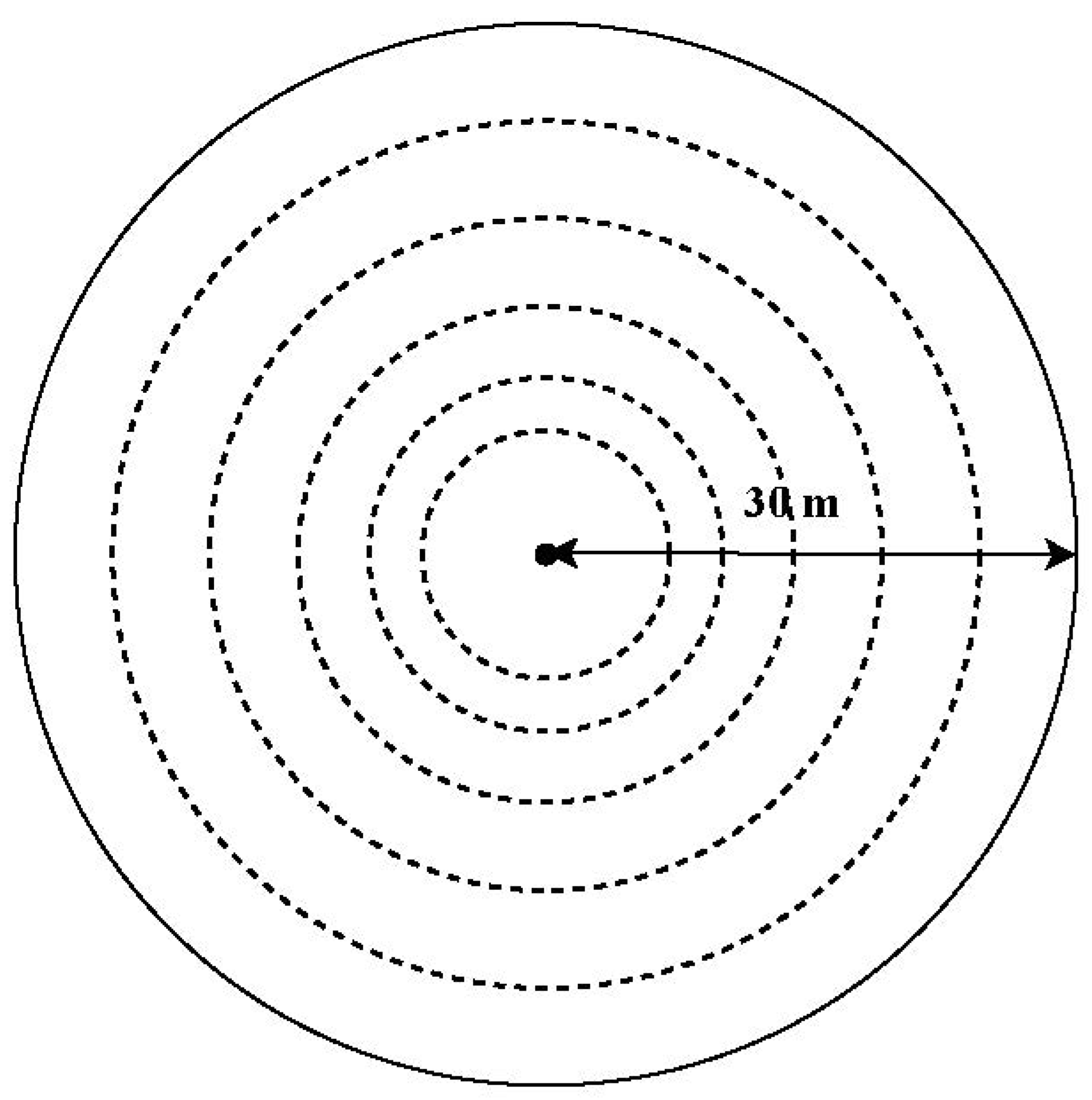
Forest experts, based on previous field experiences, guided the selection of five main plots (30 m radius; Figure 2) with trees of decay from Level 1 to Level 5 (as described in Wong et al. [44], which was inspired by Thomas’ description [4]). All plots were selected from mature forest stands. Level 1 plots consisted of totally healthy trees with no traces of decay. Leaves and branches were thickly covered in larger quantities with closed canopies. When viewed from the CIR imagery, the trees were spectrally identified via their colors (reddish to brownish). Level 2 plots consisted of early dead trees. These trees had biophysically changed in color (gray to green, from the CIR imagery) and with slight or no defoliation. The Level 3 plots also consisted of SDTs, which could be identified by their biophysical change in colors (gray to green) with more foliage and branch reduction than in Level 2. Some treetops were broken but the roots were firm in the ground. Level 4 consisted of heavily defoliated trees with several broken twigs and branches. Most of the treetops were broken while fast changing into snags. Traces of fallen tree logs were also seen on the ground, resulting in larger gaps between trees. The trees biophysically changed to dark gray in color. Snags dominated the Level 5 plots; almost all the tree branches were lost, and treetops were broken. These plots were full of deadwood; some were broken to the mid-stem level, and even beyond. Traces of fallen logs were also seen in this plot. This selection was based on visual inspections and interpretations of the ALS point clouds with their corresponding CIR images. Figure 2 shows the five plot decay levels resulting from a fusion of ALS and corresponding CIR imagery (CIR imagery was only used to support data extraction) using the Quick Terrain Modeler tool. After that, for each of these five main plots, five more sub-plots were created at radii of 5, 10, 15, 20, and 25 m, from the plots’ center, resulting in a total number of 30 plots (each decay level having six plots with a radius of 5, 10, 15, 20, 25, and 30 m; a schematic diagram is shown in Figure 3).
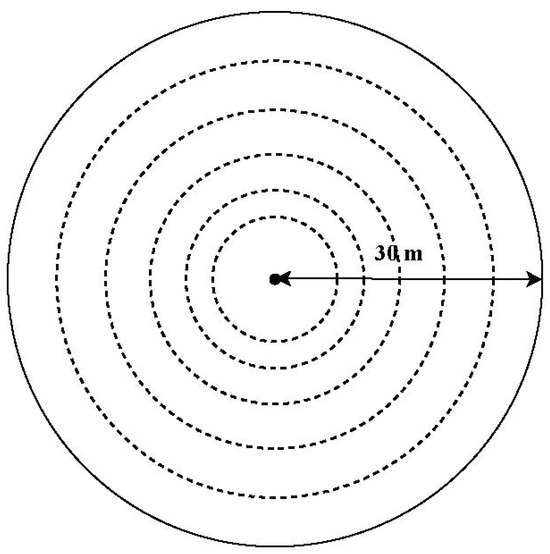
Figure 3.
Schematic illustration of the sub-plot (concentric circles in short dashes) creation for each decay level (not drawn to scale).
2.4. Point Cloud Post-Processing
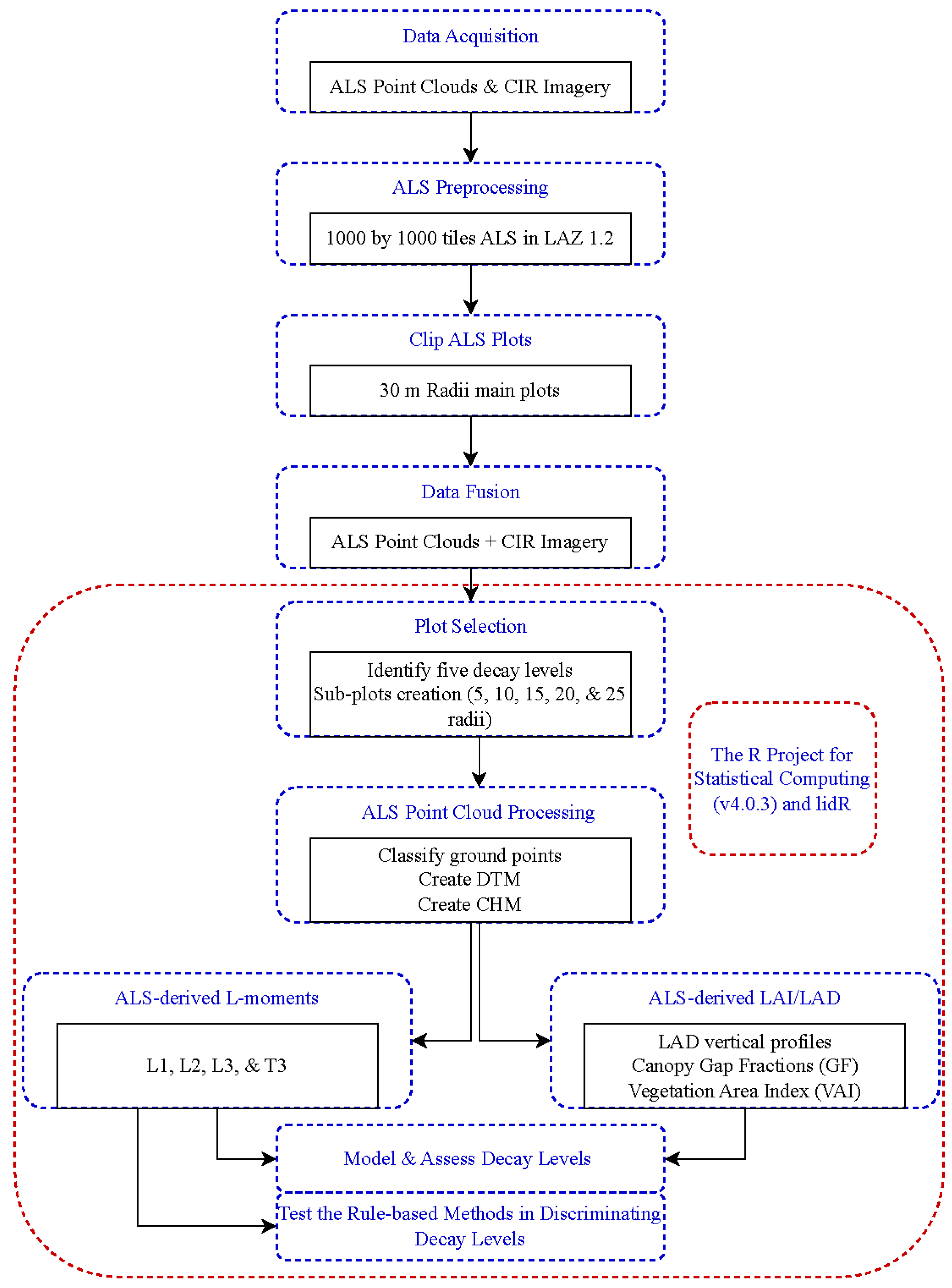
After clipping the point cloud for all selected plots, the ground points were classified using the cloth simulation function (CSF) algorithm [45]. This algorithm was considered because it demonstrated robustness on 15 samples of the ISPSR benchmark datasets with impressive accuracy. Moreover, fewer parameters were required regardless of the terrain complexity, which makes it convenient, especially for the nature of our terrain. Then, digital terrain models (DTMs) were created for each plot using the Kriging algorithm, which works in combination with the k-nearest neighbor (KNN). This algorithm was one of the most advanced for spatial data interpolation. This algorithm was considered because the processing was done on plot bases, making it manageable; otherwise, it would have been slow for larger areas due to complex computation demands, albeit with promising results. Next, the point heights were normalized with reference to the created DTMs. Finally, canopy height models (CHMs) were derived based on the Delaunay triangulation network approach at 0.5 m resolutions. Point clouds for the five main plots (30 m radius plots) were clipped and extracted using the LiDAR360 tool v5.2 (GreenValley International) while the remainder of the entire point cloud processing was done using the R-package lidR v4.0.3 [46] and the R project for statistical computing (v4.3.0). Table 1 presents some geometric ALS metrics for understanding the vertical distributions of point clouds for each of the main plots. Figure 4 illustrates the general methodology.

Table 1.
Vertical distribution of the point clouds for each plot based on geometric ALS metrics.
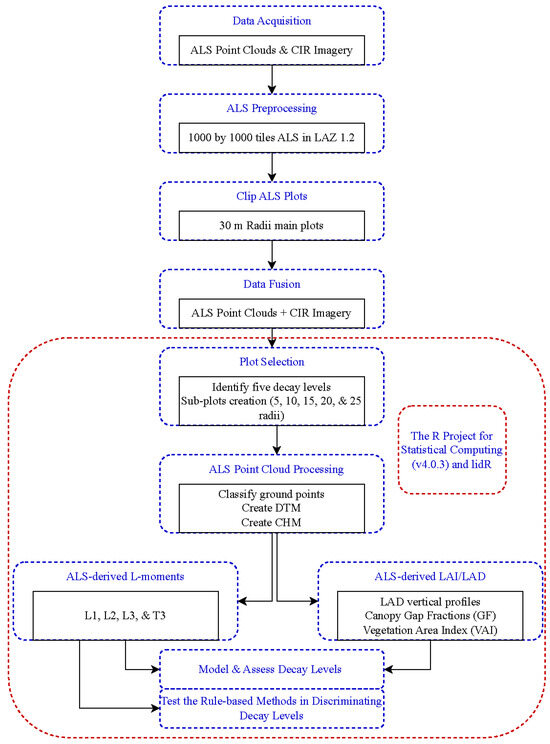
Figure 4.
The general methodological flowchart.
2.5. ALS Derived LAI/LAD
Using ALS point cloud-based data is one of the indirect approaches for measuring LAI [47], which is theoretically based on the Beer–Lambert law [47,48,49]. The canopy GF is an important variant used to derive LAI due to their close relationship with respect to a zenith angle as expressed in the Beer–Lambert law (Equation (1)) [48,49].
where GF(θ) represents the canopy gap fraction at a particular zenith angle θ, while G(θ) is the G-function of Ross Nilson [50,51,52], which denotes the fraction of a unit foliage area projected onto a perpendicular plane in the zenith direction θ. From Equation (1), we can express LAI as
LAI can be estimated using the LiDAR penetration index (LPI) with the ALS discrete return point cloud. This is based on the concept of light transmission and its attenuation through forest canopies. Light transmission through canopies attenuates depending on how dense the canopies are and their spatial distribution in the forest [53]. Thus, based on the LPI, the LAI can be estimated from the Beer–Lambert law of light extinction by estimating the fraction of light transmitted through the canopies (I/I0) with the LiDAR intensity, as expressed in Equation (3) [54,55,56,57].
where I is the light intensity below the canopy, while I0 is the total light intensity above the canopy before its penetration, and k represents the extinction coefficient. Thus, the LAI at canopy depth z (LAIz) can be expressed as [37]:
where Iz is the light intensity transmitted through the canopy at depth z. The term (Iz/I0) represents the fraction of light transmitted through the canopy at depth z, which is equivalent to the canopy GFz, from the top of the canopy to a depth z, below the canopy. This is derived from the LPI with reference to the point cloud number of returns; estimated as the ratio of the number of returns at a particular depth z below the canopy (or number of ground returns, if z is the ground) to the total number of returns [31,37,58]. Therefore, substituting GFz into Equation (4) results in:
where
where Rz is the number of returns at a particular height z below the canopies, while Rtotal is the total number of returns. If z is the ground, then the Rz becomes the total number of ground returns.
The estimation of the extinction coefficient k in comparative studies of direct measurements of LAI (field-based, using hemispherical photographs) with the light transmission approaches (LiDAR-based) has established that k is determined based on some factors like the radiation direction, the distribution of the leaf angles, and the canopy structure [59]. Research in the past years has narrated different values for the extinction coefficient, ranging from 0.28 to 0.67, from different forest types (both deciduous and coniferous) [37,59,60,61]. Aubin et al. [62], for example, reported extinction coefficients for different types of forest, strata, vegetation, and canopy cover percentages in the upper stratum, and for general use. It has been established that an extinction coefficient of approximately k = 0.5 can be used conveniently for canopies with spherical leaf inclination angle distribution [60,63]. Richardson et al. [55] reported approximate extinction coefficient values between 0.45 and 0.52 at a 95% confidence interval for a mixed coniferous-dominated forest. This corroborates the findings of Aubin et al. [62], who recommended 0.52 as the extinction coefficient for closed conifer forests. Previous research has also sanctioned the convenience assumption of spherical leaf angle distribution [64,65]. Consequently, the extinction coefficient for assuming spherical leaf angle and random foliage distribution has been widely used for calculating LAI/LAD [64,66]. Thus, in this study, we equally used k = 0.5 in deriving the LAI/LAD and GF for each decay level above 3 m heights (i.e., points from the ground to 3 m heights were not involved in the estimation) with 2 m height intervals (i.e., from the 3 m height, the trees were vertically partitioned into 2 m thickness until the maximum height in the plot) using Equation (5) [37]. Then, we analyzed the vertical profiles of the canopies in the selected plots to assess and characterize the decay levels. The relationship between LAI and LAD is expressed in Equation (7) [67,68].
where hmin represents the minimum tree height, and hmax represents the maximum tree height.
2.6. ALS-Derived L-Moments
L-moments and L-moment ratios, as an alternative to the conventional moments, are sets of statistically derived metrics based on linear combinations of order statistics that are less subject to bias and very reliable even at a small sample size, which sometimes provide even more accurate estimates than the maximum likelihood estimates [69,70]. For a random variable X with a cumulative distribution function F(x) and quantile function x(F), a sample order statistic of a random sample size r, Xk:r, can be drawn from the distribution of X [71]. Thus, L-moments of X are based on their expected values E(Xk:r). Therefore, the first, second, and third L-moments can be expressed as in Equations (8)–(10), respectively [69,70]:
Thus, for ALS-based forest structural estimations with L-moments, X represents the ALS height distributions of trees in the forest. Valbuena et al. [71] showed that the L-coefficient of variation (Lcv), which is equivalent to the Gini coefficient (GC), and the L-Skewness (Lskew) are types of the L-moment ratios, such that:
and
With these L-moment properties, they proposed two rule-based methods, Lcv = 0.5 (this threshold was considered because it represents the maximum entropy of tree sizes [72]) and Lskew = 0, for detecting tree size discrimination and light availability based on acquired ALS height returns. While the L-moments ratios are used for modeling forest plot decay levels, the proposed rules are also tested for classifying forest plot decay levels.
2.7. Relationships between the L-Moment Ratios, Vegetation Area Index, and Gap Fraction in Modeling Plot Decay Levels
We mutually evaluated the relationship between the VAI, GF, and L-moments in characterizing and modeling forest plot decay levels from ALS height returns. The VAI for each decay level was calculated by summating the LAI (all 2 m thickness) for each plot. Similarly, we calculated the average GFs for each plot. Bivariate linear regression models were built to mutually evaluate the relationship between VAI, GF, and L-moment properties in characterizing forest plot decay levels from ALS height returns. Through scatter plots of the plot decay levels 1–5, two models, regression of GF on VAI, and regression of the third L-moment ratio (T3) on VAI, were described using Equation (13), to assess the trend of decay levels and relationships with the VAI, GF, and the L-moment ratios.
where β0 represents the intercept of the best-fit line, β1 represents the slope of the best-fit line, and δ is the residual. The model’s coefficients (intercept and slope) were derived from the best-fit line through the scatter plots of decay levels. Further, the coefficient of determination (R2) was calculated and adjusted to assess the variation in proportion explained by the models. The estimations were observed at a 95% confidence interval.
2.8. Testing the Rule-Based Method for Classifying Plot Decay Levels from ALS Height Returns
We further tested the rule-based method to ascertain its veracity in classifying plot decay levels. Thus, we applied the two rules (Lcv = 0.5, and Lskew = 0) proposed by Valbuena et al. [71] with the same threshold with the presumption that Lcv = 0.5 classifies the plot decay levels into two groups (presumably Level 1 against other levels) due to variations in plot pattern and canopy sizes, while Lskew = 0 classifies two groups of decay levels based on the amount of light intensity that could reach sub-canopy levels (presumably Level 1 against other levels). As Lskew = 0 describes the symmetry of the ALS height distribution, Lskew > 0 should represent areas where light could easily reach sub-canopies, while Lskew < 0 should represent areas of closed canopies, where most ALS light pulses are backscattered by upper canopies [73].
3. Results
3.1. Characterizing Plot Decay Levels by LAD Vertical Profile Estimates
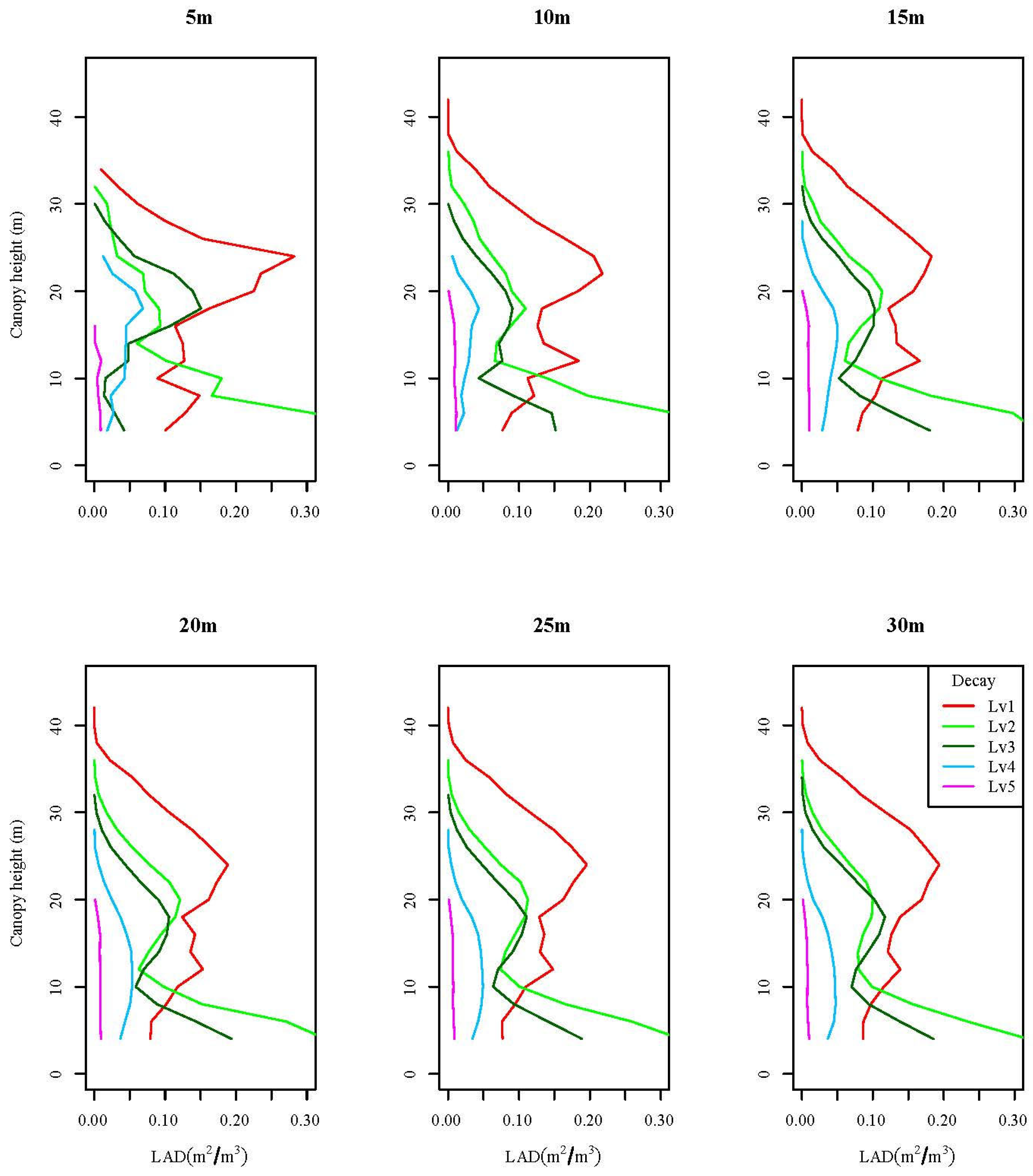
Figure 5 shows the LAD vertical profiles of the 30 plots (at varied radii, 5–30 m) of varying decay levels (Levels 1–5) from ALS height returns. Visual display of the LAD profiles clearly shows the variations in plots according to their decay levels. Noticeably, decay Level 1 (red) plots look more outstanding compared to other decay levels in all plot sizes, albeit the 5 m radius plot slightly varies. The gaps between the profiles show the variations in canopy heights, and area density. Furthermore, a close relationship is seen between Level 2 and Level 3 (green and dark green respectively) in all but the 5 m radius plots, indicating a slight decline from Level 2 to Level 3. Likewise, both levels show spread towards the right at canopy heights 3–15 m of the vertical profile. However, this observation is not the same for Levels 1, 4, and 5.
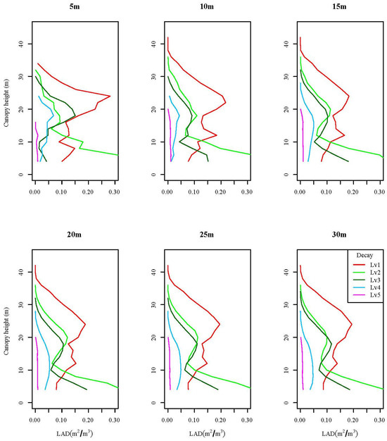
Figure 5.
LAD vertical profiles of plot decay levels at varied radii (5, 10, 15, 20, 25, and 30 m).
3.2. Relationship between VAI, GF, and L-Moment Ratios in Modeling Plot Decay Levels
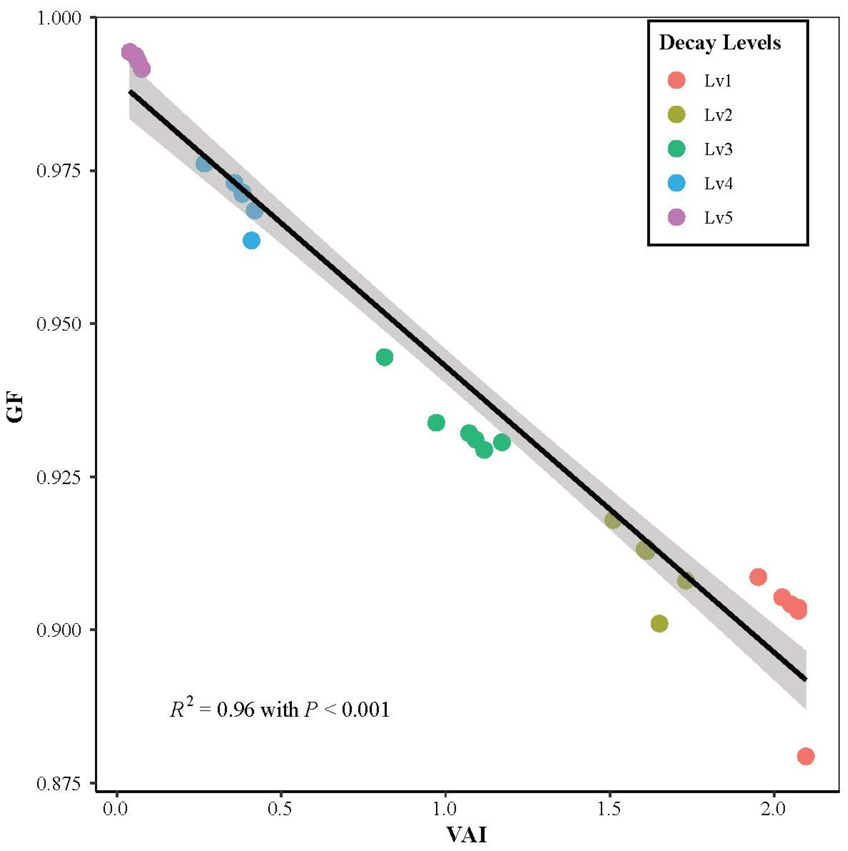
Figure 6 illustrates the relationship between VAI and GF in modeling plot decay levels from ALS height returns. Visually displayed in the figure is a scatter plot of decay Level 1 (red), Level 2 (dark khaki), Level 3 (green), Level 4 (blue), and Level 5 (purple). A bivariate regression line (black line), at a 95% confidence level (light gray), through the decay levels indicates the existence of a linear model showing a consistent decrease in GF while the VAI increases from decay Level 5 to Level 1. A total of 96% of the variation in GF was explained by the VAI with a significant negative association (VAI (slope) = −0.047, (p < 0.001)) reaching a coefficient determinant of R2 = 0.96. Table 2 shows the coefficients and confidence intervals of the adjusted model.
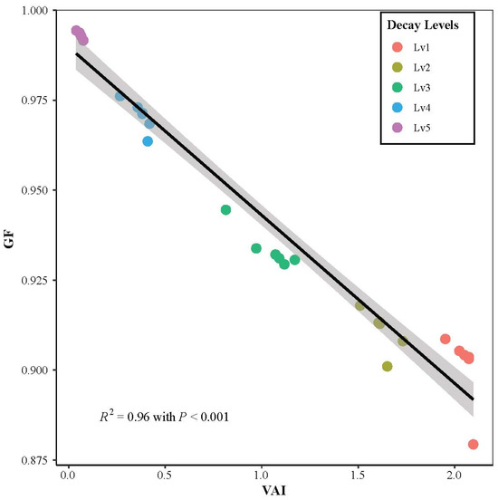
Figure 6.
The relationship between VAI and GF in modeling plot decay levels (black line) at a 95% confidence interval (light gray around the line of best fit).
Table 2.
Coefficients and confidence interval of the regression of GF on VAI in modeling plot decay levels.
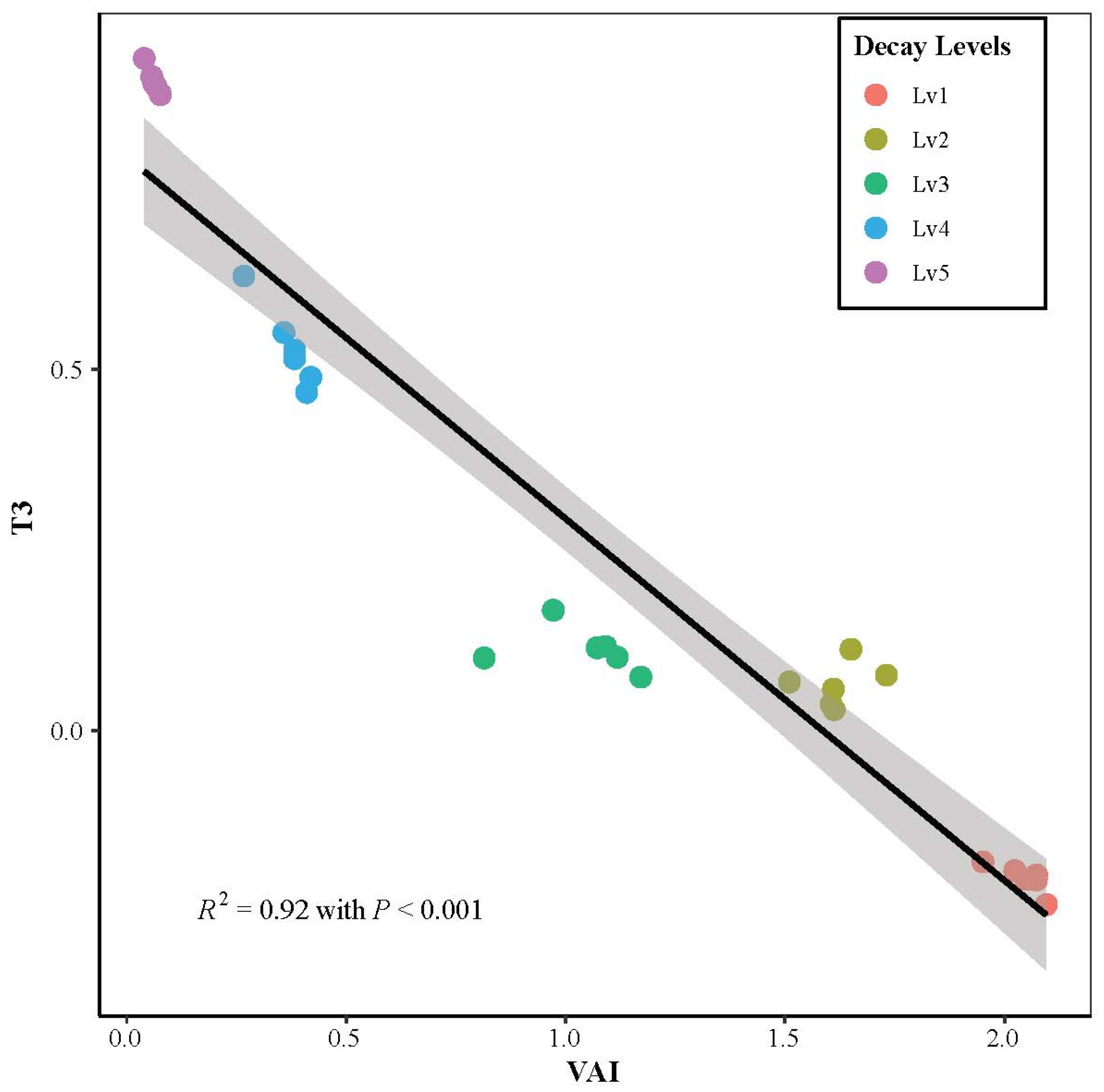
Figure 7 displays the relationship between VAI and the third L-moment ratio, which equals the L-skewness, (T3) in modeling plot decay levels from ALS height returns. The scatter plot of decay from Level 1 (red) to Level 5 (purple) is visually displayed in the figure. The bivariate regression (black line), at a 95% confidence level, through the decay levels shows the existence of a linear model decreasing consistently in T3 as the VAI increases from decay Level 5 to Level 1. In total, 92% of the variation in T3 was explained by the VAI with a significant negative association (VAI (slope) = −0.50, (p < 0.001)) reaching a coefficient determinant of R2 = 0.92. Table 3 shows the coefficients and confidence intervals of the adjusted model.
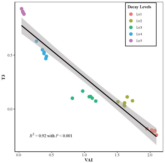
Figure 7.
The relationship between VAI and T3 in modeling plot decay levels (black line) at a 95% confidence interval (light gray around the line of best fit).
Table 3.
Coefficients and confidence intervals of the regression of T3 on VAI in modeling plot decay levels.
3.3. Testing the Rule-Based Method for Classifying Plot Decay Levels
The two rules (Lcv = 0.5, and Lskew = 0) proposed by Valbuena et al. [71] were tested to observe their effect in classifying forest plot decay levels from ALS heights returns. Both rules, based on L-moments, represent thresholds that classify the plot decay levels into two classes. Figure 8a displays the result of the first rule (Lcv = 0.5) seeking to demonstrate the classification of decay levels by the threshold based on the variation in canopy size and structure, while Figure 8b displays the result of the second rule (Lskew = 0) seeking to demonstrate the classification of plot decay levels by the threshold based on the canopy closure/density. From Equations (11) and (12), the rules become L2 = 1/2L1 and L3 = 0 respectively for the first and second rules. The short dashes represent the thresholds that separate the decay levels into two classes. On one hand, from Figure 8a, it can be observed that the threshold separates decay Levels 3, 4, and 5 at Lcv > 0.5 against the healthy and early dead trees (Level 1 and 2 respectively at Lcv < 0.5), albeit two plots from Level 3 are seen to veer off the threshold. On the other hand, Figure 8b shows clear discrimination between decay Level 1 (healthy, at Lskew < 0) and all other levels (2–5, at Lskew > 0) from the threshold, which represents the line of symmetry. It is equally worth noting the closeness of Levels 2 and 3 in both rules.
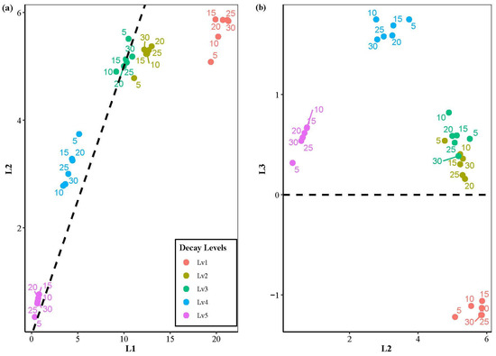
Figure 8.
Classification of plot decay levels based on the rule-based methods in the BFNP, (a) graph of the first rule-based method (short dashes represent the threshold, Lcv = 0.5); (b) graph of the second rule-based method (short dashes represent the threshold, Lskew = 0); the numbers indicated in the graph by the plots are the radii for respective plots.
4. Discussion
4.1. ALS-Based LAD Vertical Profiles Characterize Plot Decay Levels
Over decades now, researchers and forest experts have used ALS to conduct numerous forest and canopy cover investigations based on the estimation of LAI/LAD and GF [27,33,47]. While some of these studies have focused on the improvement in LAI/LAD estimation via comparison of different sensors and approaches [34,55], others considered the estimation of LAI/LAD for mapping canopy cover [31,66], defoliation, and canopy gap fractions [17,56,74]. However, to the best of our knowledge, no studies have considered the integration of LAI/LAD in characterizing and modeling forest plot decay levels. Cognizant of the fact that the declining and biophysical changes in forest plot decay would reveal the difference between each of the decay levels, this study hypothesized, due to the penetration capability of LiDAR, that ALS height returns could characterize and model forest plot decay levels.
We evaluated and characterized five decay levels (Figure 2 and Section 2.3) from the BFNP by estimating the LAD vertical profiles for thirty plots of varying radii (5, 10, 15, 20, 25, and 30 m). Each of the decay classes had six plots of varying radii (5–30 m). Findings from the results show that ALS-derived LAD vertical profiles significantly characterize forest plot decay levels (Figure 5). Evidently from Figure 5, decay Level 1 (consisting of healthy trees) was outstanding compared to Levels 2–4, and this was consistent for all plots of varying radii, albeit with a little difference for the 5m radius plot. The variation in LAD estimates through the canopy heights equally confirms this. Although the difference between decay Levels 2 and 3 could be seen, the findings also indicate that the decomposition rate between the two was not much, as this could be realized by the close relationship in the LAD vertical profiles. Interestingly, the lower parts of the profiles for both Levels (2 and 3) spread out at canopy heights 3–15 m, indicating the existence of understory young trees, which further signifies the existence of open gap spaces [12,75], possibly resulting from either canopy shrinkages or/and foliage reduction that enabled ALS pulses to reach understory, as the foliage density and compaction influences the light absorption in the canopies [55,76]. Conversely, this spread out in the vertical profile was not seen for decay Levels 1, 4, and 5. This could be understandable for Levels 4 and 5 because these were severely decayed plots, without understory trees, to the extent that almost all the trees had turned into snags and stumps (with virtually no foliage as most parts of the ground were exposed to the sky (Figure 2), another reason why 66.5% and 88.5% of the ALS point clouds, respectively, returned as ground points, Table 1). Thus, despite the vast open gap space [12,75] available for the ALS pulses to reach the understory, spread out would not be seen in the profile. However, Level 1 should have some understory trees, yet this was not detected because the ALS pulses were unable to reach understory levels (closed gap spaces [12,75]) due to the closed canopy which rendered the pulses backscattered from the higher canopies.
Furthermore, the vertical profiles of the five decay Levels show a consistent decline both in the LAD estimates and height, indicating a strong correlation. The apparent inference in the decline in canopy height is breakages (i.e., broken tops or broken stems), especially for Levels 4 and 5. While this finding confirms the plausibility of using ALS height returns only, for examining above-ground biomass and carbon dynamics [77], it is equally significant for identifying and mapping forest areas that have large gaps for forest resource management and planning (e.g., decay Levels 4 and 5 could serve as fuels), especially in cloudy forest regions with limited access.
4.2. Modeling Plot Decay Levels Significantly Explained the Decay Trend and the Relationship between VAI, GF, and L-Moments
While assessing the relationships between VAI, GF, and L-moments ratio, we modeled the plot decay levels from ALS height returns using bivariate linear regressions. All the LAIs computed at each stratum (2 m thickness in height) of a plot summed up constituted the VAI whereas GF was the average canopy gap fraction. The third L-moment ratio (T3), also known to measure the skewness, was the ratio of the third to second L-moment (L3/L2). The relationship between VAI and GF (Figure 6) and VAI and T3 (Figure 7) resulted in linear models that significantly explained the dynamics of the five plot decay levels with a negative slope from Level 5 to Level 1. While 96% of the variation in GF was explained by the VAI with a significant negative association (VAI (slope) = −0.047, (p < 0.001)), 92% of the variation in T3 was explained by the VAI, also with a significant negative association (VAI (slope) = −0.50, (p < 0.001)); both at 95% confidence interval. Table 2 and Table 3 display the coefficient values (intercepts and slopes) of the regressions (first and second models respectively), with their confidence intervals and p−values. Findings from both models show a clear indication of the declining trend of plot decay levels through the regression with strong correlations achieving coefficients of determination reaching R2 = 0.96 and R2 = 0.92 for the first and second models respectively. Thus, both models can be used to predict forest plot decay levels, based on plot VAIs. Furthermore, with the VAI, the first model can equally predict the GF, while the second model also predicts the skewness of the respective decayed plots. The practical implication of these findings is that, especially in forests that have limited access and in cloudy weather conditions, forest managers can use ALS height returns to model forest plot decay levels. This leads to the understanding of forest growth dynamics for effective forest management.
4.3. Rule-Based Methods Classify Healthy and Deadwood Plots
ALS-derived L-moments directly detect forest structural features [71,78]. Valbuena et al. [71] proposed two rules; the first rule (Lcv = 0.5) was for classifying even-size forest areas (Lcv < 0.5) and areas dominated by great tree size inequality (Lcv > 0.5), whereas the second rule (Lskew = 0) was for classifying open canopy forest areas (Lskew > 0) and closed canopy forest areas (Lskew < 0). Cognizant of the fact that the effect of tree decay results in biophysical changes in tree canopy structure and sizes (due to defoliation, broken tops and stems, broken twigs and branches, and shrinkages), we hypothesized that ALS-derived L-moments can directly classify forest plot decay levels to serve as a convenient approach to understanding forest growth dynamics in the absence of field data. This is due to the changes that arise over time resulting from structural deficiency as the dead trees continuously decay (Wong et al. [44]), which equally explains the fact that the variations in plot decay levels result in great tree size inequalities. Consequently, we tested the two rules for classifying forest plot decay levels from ALS height return using the derived L-moments.
On one hand, our findings (Figure 8a) showed that the first rule classified the most severely decayed plots (Levels 3, 4, and 5) as areas of great size inequality (Lcv > 0.5) while the healthy and early dead plots (Levels 1 and 2 respectively) were classified as even-sized areas (Lcv < 0.5). This indicates that the first rule has the potential to classify deadwood plots from plots constituting declining (early dead plots) and healthy trees. It is worth noting that, although decay Level 2 is classified as even-sized areas, it is closer to Level 3. While this indicates a small difference between Level 2 and 3, it further confirms that the Level 2 plots are early-stage dead trees, which may have a slight structural deficiency contrary to Levels 3, 4, and 5. This also demonstrates the reason why it is sometimes challenging to differentiate between Level 2 and 3, and 1 and 2 from only ALS point clouds; thus, showing the necessity of the sensor combination in assessing decay levels (Wong et al., [44].) Moreover, the findings indicate that there exists a dependency between the L1 (mean ALS height) and the L2 as the declining trend in decay levels is demonstrated in Figure 8a, which equally reflects the decline in tree heights from decay Levels 1 to 5. This further implies that ALS-derived L-moments, especially the relationship between L1 and L2, have the potential for modeling forest plot decay levels.
On the other hand, the second rule (Lskew = 0) classified decay Level 1 as closed canopy areas (Lskew < 0), while Levels 2–5 are classified as open canopy areas (Lskew > 0), Figure 8b. It is noteworthy that positive skewness is seen for all dead plots, which have at least some structural deficiency (resulting in open canopy and increasing GF), while negative skewness is seen for structurally healthy plots (dense and closed canopy). This corroborates the concept of forest plot decay levels and their effects. For example, dense forests with healthy trees (Level 1) have closed canopies. However, when trees die and begin to decay, gaps begin to widen in proportion to the degree of decay. Thus, the distribution of ALS height returns through the second rule has potential for discriminating healthy plots (where ALS pulses are unable to reach understory as they are mostly backscattered from the higher canopy due to closeness; these are forest areas termed as euphotic zone ([12,75]) from decayed plot (where ALS pulses mostly reach understory canopy and ground due to increasing GF and openness; these areas are termed as the oligophotic zone ([12,75]).
These findings show that the derived L-moment rule-based methods look promising, especially for classifying healthy and deadwood plots of varying decay levels directly from ALS height returns. This can be a simple and convenient approach forest managers can adopt to assess and understand forest growth dynamics for effective management. Moreover, forest managers can exploit this approach to map out gap areas for managing forest resources. The approach can equally be significant for assessing forest biomass, carbon stock, and biodiversity.
4.4. Limitations
Generally, despite our anticipation that the proposed method in this study can have significant practical value for effective forest management and planning of resources, we equally must acknowledge the limitation of few experimental data available at our disposal. Thus, we tried to make up for this limitation by varying the sample plot size. Notwithstanding, this study can serve as a basis for improved and advanced research in the future.
5. Conclusions
In this study, we proposed a practically significant method for understanding forest growth dynamics for effective planning and management of forest resources. We characterized and modeled five decay levels of forest plots in the BFNP based on LAI, GF, and L-moments from ALS height returns only through assessments of point cloud dispersions and skewness. First, we characterized forest plot decay levels by estimating their LAD vertical profiles. Findings from the profiles show a clear decline in LAD and heights from Level 1 to 5. Also, we modeled the plot decay levels while assessing the relationship between VAI and GF as well as VAI and T3 (third L-moment ratio) on respective plots with bivariate regression. The models significantly explained the declining trend in decays with coefficients of determination reaching R2 = 0.96 (GF on VAI) and R2 = 0.92 (T3 on VAI) at a 95% confidence interval. Furthermore, we tested two rule-based methods (Lcv = 0.5 and Lskew = 0) proposed in the literature to classify plot decay levels into two groups: healthy plots (Level 1) and deadwood plots (Level 2–5). However, we found that while the second rule (Lskew = 0) works perfectly, the first rule categorized the healthy and early dead plots in one category, although there was a wide distance between the two as the early dead plots were closer to the threshold boundary. These findings are very significant for understanding the decay levels and forest growth dynamics. This can equally serve as a convenient, cost-effective approach for forest managers to assess and estimate the biomass, carbon stock, and biodiversity from ALS height returns without field data. Moreover, forest managers can exploit the approach for mapping forest gaps for planning and managing forest resources for effective forest management and preservation, especially in cloudy temperate forest regions having limited access.
Author Contributions
Conceptualization, A.S.-M. and W.Y.; methodology, A.S.-M.; software, A.S.-M.; validation, A.S.-M. and T.C.W.; formal analysis, A.S.-M.; investigation, A.S.-M.; resources, W.Y. and M.H.; data curation, A.S.-M. and T.C.W.; writing—original draft preparation, A.S.-M.; writing—review and editing, A.S.-M., R.F., W.Y. and M.H.; visualization, A.S.-M. and T.C.W.; supervision, W.Y.; project administration, W.Y; funding acquisition, A.S.-M. and W.Y. All authors have read and agreed to the published version of the manuscript.
Funding
This research was funded by the “National Natural Science Foundation of China, grant number 42171361” and the “Research Grant Council of the Hong Kong Special Administration Region, China, under PolyU, grant number 25211819”.
Data Availability Statement
The corresponding author will make the data available upon reasonable request.
Conflicts of Interest
The authors declare no conflicts of interest.
References
- Lausch, A.; Heurich, M.; Fahse, L. Spatio-Temporal Infestation Patterns of Ips typographus (L.) in the Bavarian Forest National Park, Germany. Ecol. Indic. 2013, 31, 73–81. [Google Scholar] [CrossRef]
- Sani-Mohammed, A.; Yao, W.; Heurich, M. Instance Segmentation of Standing Dead Trees in Dense Forest from Aerial Imagery Using Deep Learning. ISPRS Open J. Photogramm. Remote Sens. 2022, 6, 100024. [Google Scholar] [CrossRef]
- Keen, F.P. The Rate of Natural Falling of Beetle-Killed Ponderosa Pine Snags. J. For. 1955, 53, 720–723. [Google Scholar]
- Thomas, J.W. (Ed.) Wildlife Habitats in Managed Forests: The Blue Mountains of Oregon and Washington; US Department of Agriculture: Washington, DC, USA, 1979; Volume 553.
- Lechner, A.M.; Foody, G.M.; Boyd, D.S. Applications in Remote Sensing to Forest Ecology and Management. One Earth 2020, 2, 405–412. [Google Scholar] [CrossRef]
- Garrity, S.R.; Allen, C.D.; Brumby, S.P.; Gangodagamage, C.; McDowell, N.G.; Cai, D.M. Quantifying Tree Mortality in a Mixed Species Woodland Using Multitemporal High Spatial Resolution Satellite Imagery. Remote Sens. Environ. 2013, 129, 54–65. [Google Scholar] [CrossRef]
- Gonzalez, P.; Asner, G.; Battles, J.; Lefsky, M.; Waring, K.; Palace, M. Forest Carbon Densities and Uncertainties from Lidar, QuickBird, and Field Measurements in California. Remote Sens. Environ. 2010, 114, 1561–1575. [Google Scholar] [CrossRef]
- Polewski, P.; Shelton, J.; Yao, W.; Heurich, M. Instance Segmentation of Fallen Trees in Aerial Color Infrared Imagery Using Active Multi-Contour Evolution with Fully Convolutional Network-Based Intensity Priors. ISPRS J. Photogramm. Remote Sens. 2021, 178, 297–313. [Google Scholar] [CrossRef]
- Polewski, P.; Yao, W.; Heurich, M.; Krzystek, P.; Stilla, U. Detection of Fallen Trees in ALS Point Clouds Using a Normalized Cut Approach Trained by Simulation. ISPRS J. Photogramm. Remote Sens. 2015, 105, 252–271. [Google Scholar] [CrossRef]
- Polewski, P.; Yao, W.; Heurich, M.; Krzystek, P.; Stilla, U. A Voting-Based Statistical Cylinder Detection Framework Applied to Fallen Tree Mapping in Terrestrial Laser Scanning Point Clouds. ISPRS J. Photogramm. Remote Sens. 2017, 129, 118–130. [Google Scholar] [CrossRef]
- Ramsey, E.; Rangoonwala, A.; Chi, Z.; Jones, C.E.; Bannister, T. Marsh Dieback, Loss, and Recovery Mapped with Satellite Optical, Airborne Polarimetric Radar, and Field Data. Remote Sens. Environ. 2014, 152, 364–374. [Google Scholar] [CrossRef]
- Lefsky, M.A.; Cohen, W.B.; Parker, G.G.; Harding, D.J. Lidar Remote Sensing for Ecosystem Studies. BioScience 2002, 52, 19–30. [Google Scholar] [CrossRef]
- Dubayah, R.O.; Drake, J.B. Lidar Remote Sensing for Forestry. J. For. 2000, 98, 44–46. [Google Scholar] [CrossRef]
- Dong, P.; Chen, Q. LiDAR Remote Sensing and Applications; CRC Press: Boca Raton, FL, USA, 2017; ISBN 978-1-351-23335-4. [Google Scholar]
- Yao, W.; Krzystek, P.; Heurich, M. Tree Species Classification and Estimation of Stem Volume and DBH Based on Single Tree Extraction by Exploiting Airborne Full-Waveform LiDAR Data. Remote Sens. Environ. 2012, 123, 368–380. [Google Scholar] [CrossRef]
- Teobaldelli, M.; Cona, F.; Saulino, L.; Migliozzi, A.; D’Urso, G.; Langella, G.; Manna, P.; Saracino, A. Detection of Diversity and Stand Parameters in Mediterranean Forests Using Leaf-off Discrete Return LiDAR Data. Remote Sens. Environ. 2017, 192, 126–138. [Google Scholar] [CrossRef]
- Heiskanen, J.; Korhonen, L.; Hietanen, J.; Pellikka, P.K.E. Use of Airborne Lidar for Estimating Canopy Gap Fraction and Leaf Area Index of Tropical Montane Forests. Int. J. Remote Sens. 2015, 36, 2569–2583. [Google Scholar] [CrossRef]
- Falkowski, M.J.; Evans, J.S.; Martinuzzi, S.; Gessler, P.E.; Hudak, A.T. Characterizing Forest Succession with Lidar Data: An Evaluation for the Inland Northwest, USA. Remote Sens. Environ. 2009, 113, 946–956. [Google Scholar] [CrossRef]
- Asner, G.P.; Mascaro, J. Mapping Tropical Forest Carbon: Calibrating Plot Estimates to a Simple LiDAR Metric. Remote Sens. Environ. 2014, 140, 614–624. [Google Scholar] [CrossRef]
- Gu, Z.; Cao, S.; Sanchez-Azofeifa, G.A. Using LiDAR Waveform Metrics to Describe and Identify Successional Stages of Tropical Dry Forests. Int. J. Appl. Earth Obs. Geoinf. 2018, 73, 482–492. [Google Scholar] [CrossRef]
- Shi, Y.; Wang, T.; Skidmore, A.K.; Heurich, M. Important LiDAR Metrics for Discriminating Forest Tree Species in Central Europe. ISPRS J. Photogramm. Remote Sens. 2018, 137, 163–174. [Google Scholar] [CrossRef]
- Soto, G.E.; Pérez-Hernández, C.G.; Hahn, I.J.; Rodewald, A.D.; Vergara, P.M. Tree Senescence as a Direct Measure of Habitat Quality: Linking Red-Edge Vegetation Indices to Space Use by Magellanic Woodpeckers. Remote Sens. Environ. 2017, 193, 1–10. [Google Scholar] [CrossRef]
- Putman, E.B.; Popescu, S.C.; Eriksson, M.; Zhou, T.; Klockow, P.; Vogel, J.; Moore, G.W. Detecting and Quantifying Standing Dead Tree Structural Loss with Reconstructed Tree Models Using Voxelized Terrestrial Lidar Data. Remote Sens. Environ. 2018, 209, 52–65. [Google Scholar] [CrossRef]
- Klockow, P.A.; Putman, E.B.; Vogel, J.G.; Moore, G.W.; Edgar, C.B.; Popescu, S.C. Allometry and Structural Volume Change of Standing Dead Southern Pine Trees Using Non-Destructive Terrestrial LiDAR. Remote Sens. Environ. 2020, 241, 111729. [Google Scholar] [CrossRef]
- Chen, J.M.; Black, T.A. Defining Leaf Area Index for Non-Flat Leaves. Plant Cell Environ. 1992, 15, 421–429. [Google Scholar] [CrossRef]
- Lang, A.R.G. Application of Some of Cauchy’s Theorems to Estimation of Surface Areas of Leaves, Needles and Branches of Plants, and Light Transmittance. Agric. For. Meteorol. 1991, 55, 191–212. [Google Scholar] [CrossRef]
- Weiss, M.; Baret, F.; Smith, G.J.; Jonckheere, I.; Coppin, P. Review of Methods for in Situ Leaf Area Index (LAI) Determination Part II. Estimation of LAI, Errors and Sampling. Agric. For. Meteorol. 2004, 121, 37–53. [Google Scholar] [CrossRef]
- Hosoi, F.; Omasa, K. Voxel-Based 3-D Modeling of Individual Trees for Estimating Leaf Area Density Using High-Resolution Portable Scanning Lidar. IEEE Trans. Geosci. Remote Sens. 2006, 44, 3610–3618. [Google Scholar] [CrossRef]
- Hosoi, F.; Omasa, K. Factors Contributing to Accuracy in the Estimation of the Woody Canopy Leaf Area Density Profile Using 3D Portable Lidar Imaging. J. Exp. Bot. 2007, 58, 3463–3473. [Google Scholar] [CrossRef]
- Korhonen, L.; Morsdorf, F. Estimation of Canopy Cover, Gap Fraction and Leaf Area Index with Airborne Laser Scanning. In Forestry Applications of Airborne Laser Scanning: Concepts and Case Studies; Maltamo, M., Næsset, E., Vauhkonen, J., Eds.; Springer: Dordrecht, The Netherlands, 2014; pp. 397–417. ISBN 978-94-017-8663-8. [Google Scholar]
- Morsdorf, F.; Kötz, B.; Meier, E.; Itten, K.I.; Allgöwer, B. Estimation of LAI and Fractional Cover from Small Footprint Airborne Laser Scanning Data Based on Gap Fraction. Remote Sens. Environ. 2006, 104, 50–61. [Google Scholar] [CrossRef]
- Sasaki, T.; Imanishi, J.; Ioki, K.; Song, Y.; Morimoto, Y. Estimation of Leaf Area Index and Gap Fraction in Two Broad-Leaved Forests by Using Small-Footprint Airborne LiDAR. Landsc. Ecol. Eng. 2016, 12, 117–127. [Google Scholar] [CrossRef]
- Jonckheere, I.; Fleck, S.; Nackaerts, K.; Muys, B.; Coppin, P.; Weiss, M.; Baret, F. Review of Methods for in Situ Leaf Area Index Determination Part I. Theories, Sensors and Hemispherical Photography. Agric. For. Meteorol. 2004, 121, 19–35. [Google Scholar] [CrossRef]
- Kamoske, A.G.; Dahlin, K.M.; Stark, S.C.; Serbin, S.P. Leaf Area Density from Airborne LiDAR: Comparing Sensors and Resolutions in a Temperate Broadleaf Forest Ecosystem. For. Ecol. Manag. 2019, 433, 364–375. [Google Scholar] [CrossRef]
- Ryu, Y.; Nilson, T.; Kobayashi, H.; Sonnentag, O.; Law, B.E.; Baldocchi, D.D. On the Correct Estimation of Effective Leaf Area Index: Does It Reveal Information on Clumping Effects? Agric. For. Meteorol. 2010, 150, 463–472. [Google Scholar] [CrossRef]
- Asner, G.P.; Powell, G.V.N.; Mascaro, J.; Knapp, D.E.; Clark, J.K.; Jacobson, J.; Kennedy-Bowdoin, T.; Balaji, A.; Paez-Acosta, G.; Victoria, E.; et al. High-Resolution Forest Carbon Stocks and Emissions in the Amazon. Proc. Natl. Acad. Sci. USA 2010, 107, 16738–16742. [Google Scholar] [CrossRef]
- Bouvier, M.; Durrieu, S.; Fournier, R.; Renaud, J.-P.; Saint-Geours, N.; Grau, E.; Guyon, D. Generalizing Predictive LiDAR Models of Forest Inventory Attributes Using an Area-Based Approach. In Proceedings of the FORESEE Workshop-Forestry Applications of Remote Sensing Technologies, Champenoux, France, 8–10 October 2014. [Google Scholar]
- Gobakken, T.; Næsset, E. Assessing Effects of Laser Point Density, Ground Sampling Intensity, and Field Sample Plot Size on Biophysical Stand Properties Derived from Airborne Laser Scanner Data. Can. J. For. Res. 2008, 38, 1095–1109. [Google Scholar] [CrossRef]
- Korhonen, L.; Korpela, I.; Heiskanen, J.; Maltamo, M. Airborne Discrete-Return LIDAR Data in the Estimation of Vertical Canopy Cover, Angular Canopy Closure and Leaf Area Index. Remote Sens. Environ. 2011, 115, 1065–1080. [Google Scholar] [CrossRef]
- Nielsen, M.M.; Heurich, M.; Malmberg, B.; Brun, A. Automatic Mapping of Standing Dead Trees after an Insect Outbreak Using the Window Independent Context Segmentation Method. J. For. 2014, 112, 564–571. [Google Scholar] [CrossRef]
- Müller, M.; Job, H. Managing Natural Disturbance in Protected Areas: Tourists’ Attitude towards the Bark Beetle in a German National Park. Biol. Conserv. 2009, 142, 375–383. [Google Scholar] [CrossRef]
- van der Knaap, W.O.; van Leeuwen, J.F.N.; Fahse, L.; Szidat, S.; Studer, T.; Baumann, J.; Heurich, M.; Tinner, W. Vegetation and Disturbance History of the Bavarian Forest National Park, Germany. Veg. Hist. Archaeobotany 2020, 29, 277–295. [Google Scholar] [CrossRef]
- Latifi, H.; Holzwarth, S.; Skidmore, A.; Brůna, J.; Červenka, J.; Darvishzadeh, R.; Hais, M.; Heiden, U.; Homolová, L.; Krzystek, P.; et al. A Laboratory for Conceiving Essential Biodiversity Variables (EBVs)—The ‘Data Pool Initiative for the Bohemian Forest Ecosystem’. Methods Ecol. Evol. 2021, 12, 2073–2083. [Google Scholar] [CrossRef]
- Wong, T.-C.; Sani-Mohammed, A.; Wang, J.; Wang, P.; Yao, W.; Heurich, M. Classification of Single Tree Decay Stages from Combined Airborne LiDAR Data and CIR Imagery. Geo-Spat. Inf. Sci. 2024, 1–16. [Google Scholar] [CrossRef]
- Zhang, W.; Qi, J.; Wan, P.; Wang, H.; Xie, D.; Wang, X.; Yan, G. An Easy-to-Use Airborne LiDAR Data Filtering Method Based on Cloth Simulation. Remote Sens. 2016, 8, 501. [Google Scholar] [CrossRef]
- Roussel, J.R.; Auty, D.; Coops, N.C.; Tompalski, P.; Goodbody, T.R.H.; Meador, A.S.; Bourdon, J.F.; de Boissieu, F.; Achim, A. lidR: An R Package for Analysis of Airborne Laser Scanning (ALS) Data. Remote Sens. Environ. 2020, 251, 112062. [Google Scholar] [CrossRef]
- Yan, G.; Hu, R.; Luo, J.; Weiss, M.; Jiang, H.; Mu, X.; Xie, D.; Zhang, W. Review of Indirect Optical Measurements of Leaf Area Index: Recent Advances, Challenges, and Perspectives. Agric. For. Meteorol. 2019, 265, 390–411. [Google Scholar] [CrossRef]
- Nilson, T. A Theoretical Analysis of the Frequency of Gaps in Plant Stands. Agric. Meteorol. 1971, 8, 25–38. [Google Scholar] [CrossRef]
- de Wit, C.T. Photosynthesis of Leaf Canopies; Center for Agricultural Publications and Documentation: Wageningen, The Netherlands, 1965; pp. 1–64. [Google Scholar]
- Nilson, T. Inversion of Gap Frequency Data in Forest Stands. Agric. For. Meteorol. 1999, 98–99, 437–448. [Google Scholar] [CrossRef]
- Tian, L.; Qu, Y.; Qi, J. Estimation of Forest LAI Using Discrete Airborne LiDAR: A Review. Remote Sens. 2021, 13, 2408. [Google Scholar] [CrossRef]
- Zhao, F.; Yang, X.; Schull, M.A.; Román-Colón, M.O.; Yao, T.; Wang, Z.; Zhang, Q.; Jupp, D.L.B.; Lovell, J.L.; Culvenor, D.S.; et al. Measuring Effective Leaf Area Index, Foliage Profile, and Stand Height in New England Forest Stands Using a Full-Waveform Ground-Based Lidar. Remote Sens. Environ. 2011, 115, 2954–2964. [Google Scholar] [CrossRef]
- Lee, H.; Slatton, K.C.; Roth, B.E.; Cropper, W.P. Prediction of Forest Canopy Light Interception Using Three-dimensional Airborne LiDAR Data. Int. J. Remote Sens. 2008, 30, 189–207. [Google Scholar] [CrossRef]
- Luo, S.; Wang, C.; Pan, F.; Xi, X.; Li, G.; Nie, S.; Xia, S. Estimation of Wetland Vegetation Height and Leaf Area Index Using Airborne Laser Scanning Data. Ecol. Indic. 2015, 48, 550–559. [Google Scholar] [CrossRef]
- Richardson, J.J.; Moskal, L.M.; Kim, S.H. Modeling Approaches to Estimate Effective Leaf Area Index from Aerial Discrete-Return LIDAR. Agric. For. Meteorol. 2009, 149, 1152–1160. [Google Scholar] [CrossRef]
- Solberg, S.; Næsset, E.; Hanssen, K.H.; Christiansen, E. Mapping Defoliation during a Severe Insect Attack on Scots Pine Using Airborne Laser Scanning. Remote Sens. Environ. 2006, 102, 364–376. [Google Scholar] [CrossRef]
- Wang, Y.; Fang, H. Estimation of LAI with the LiDAR Technology: A Review. Remote Sens. 2020, 12, 3457. [Google Scholar] [CrossRef]
- Hopkinson, C.; Lovell, J.; Chasmer, L.; Jupp, D.; Kljun, N.; Gorsel, E. van Integrating Terrestrial and Airborne Lidar to Calibrate a 3D Canopy Model of Effective Leaf Area Index. Remote Sens. Environ. 2013, 136, 301–314. [Google Scholar] [CrossRef]
- Bréda, N.J.J. Ground-based Measurements of Leaf Area Index: A Review of Methods, Instruments and Current Controversies. J. Exp. Bot. 2003, 54, 2403–2417. [Google Scholar] [CrossRef]
- Martens, S.N.; Ustin, S.L.; Rousseau, R.A. Estimation of Tree Canopy Leaf Area Index by Gap Fraction Analysis. For. Ecol. Manag. 1993, 61, 91–108. [Google Scholar] [CrossRef]
- Solberg, S.; Naesset, E.; Bollandsas, O.M. Single Tree Segmentation Using Airborne Laser Scanner Data in a Structurally Heterogeneous Spruce Forest. Photogramm. Eng. Remote Sens. 2006, 72, 1369–1378. [Google Scholar] [CrossRef]
- Aubin, I.; Beaudet, M.; Messier, C. Light Extinction Coefficients Specific to the Understory Vegetation of the Southern Boreal Forest, Quebec. Can. J. For. Res. 2000, 30, 168–177. [Google Scholar] [CrossRef]
- Jones, H.G. Plants and Microclimate: A Quantitative Approach to Environmental Plant Physiology; Cambridge University Press: Cambridge, UK, 1992; p. 428. [Google Scholar]
- Tang, H.; Brolly, M.; Zhao, F.; Strahler, A.H.; Schaaf, C.L.; Ganguly, S.; Zhang, G.; Dubayah, R. Deriving and Validating Leaf Area Index (LAI) at Multiple Spatial Scales through Lidar Remote Sensing: A Case Study in Sierra National Forest, CA. Remote Sens. Environ. 2014, 143, 131–141. [Google Scholar] [CrossRef]
- Vose, J.M.; Sullivan, N.H.; Clinton, B.D.; Bolstad, P.V. Vertical Leaf Area Distribution, Light Transmittance, and Application of the Beer–Lambert Law in Four Mature Hardwood Stands in the Southern Appalachians. Can. J. For. Res. 1995, 25, 1036–1043. [Google Scholar] [CrossRef]
- Solberg, S.; Brunner, A.; Hanssen, K.H.; Lange, H.; Næsset, E.; Rautiainen, M.; Stenberg, P. Mapping LAI in a Norway Spruce Forest Using Airborne Laser Scanning. Remote Sens. Environ. 2009, 113, 2317–2327. [Google Scholar] [CrossRef]
- de Almeida, D.R.A.; Stark, S.C.; Shao, G.; Schietti, J.; Nelson, B.W.; Silva, C.A.; Gorgens, E.B.; Valbuena, R.; Papa, D.d.A.; Brancalion, P.H.S. Optimizing the Remote Detection of Tropical Rainforest Structure with Airborne Lidar: Leaf Area Profile Sensitivity to Pulse Density and Spatial Sampling. Remote Sens. 2019, 11, 92. [Google Scholar] [CrossRef]
- Zhao, J.; Li, J.; Liu, Q. Review of Forest Vertical Structure Parameter Inversion Based on Remote Sensing Technology. Yaogan Xuebao J. Remote Sens. 2013, 17, 697–716. [Google Scholar] [CrossRef]
- Hosking, J.R.M. L-Moments: Analysis and Estimation of Distributions Using Linear Combinations of Order Statistics. J. R. Stat. Soc. Ser. B Methodol. 1990, 52, 105–124. [Google Scholar] [CrossRef]
- Hosking, J.R.M. Some Theoretical Results Concerning L-Moments; Research Report RC 14492; IBM Thomas J. Watson Research Division: Yorktown Heights, NY, USA, 1989; pp. 1–9. [Google Scholar]
- Valbuena, R.; Maltamo, M.; Mehtätalo, L.; Packalen, P. Key Structural Features of Boreal Forests May Be Detected Directly Using L-Moments from Airborne Lidar Data. Remote Sens. Environ. 2017, 194, 437–446. [Google Scholar] [CrossRef]
- Valbuena, R.; Packalén, P.; Martı´n-Fernández, S.; Maltamo, M. Diversity and Equitability Ordering Profiles Applied to Study Forest Structure. For. Ecol. Manag. 2012, 276, 185–195. [Google Scholar] [CrossRef]
- Valbuena, R.; Packalen, P.; Mehtätalo, L.; García-Abril, A.; Maltamo, M. Characterizing Forest Structural Types and Shelterwood Dynamics from Lorenz-Based Indicators Predicted by Airborne Laser Scanning. Can. J. For. Res. 2013, 43, 1063–1074. [Google Scholar] [CrossRef]
- Solberg, S. Mapping Gap Fraction, LAI and Defoliation Using Various ALS Penetration Variables. Int. J. Remote Sens. 2010, 31, 1227–1244. [Google Scholar] [CrossRef]
- Lefsky, M.A.; Cohen, W.B.; Acker, S.A.; Parker, G.G.; Spies, T.A.; Harding, D. Lidar Remote Sensing of the Canopy Structure and Biophysical Properties of Douglas-Fir Western Hemlock Forests. Remote Sens. Environ. 1999, 70, 339–361. [Google Scholar] [CrossRef]
- Stark, S.C.; Leitold, V.; Wu, J.L.; Hunter, M.O.; de Castilho, C.V.; Costa, F.R.C.; Mcmahon, S.M.; Parker, G.G.; Shimabukuro, M.T.; Lefsky, M.A.; et al. Amazon Forest Carbon Dynamics Predicted by Profiles of Canopy Leaf Area and Light Environment. Ecol. Lett. 2012, 15, 1406–1414. [Google Scholar] [CrossRef]
- Drake, J.B.; Dubayah, R.O.; Knox, R.G.; Clark, D.B.; Blair, J.B. Sensitivity of Large-Footprint Lidar to Canopy Structure and Biomass in a Neotropical Rainforest. Remote Sens. Environ. 2002, 81, 378–392. [Google Scholar] [CrossRef]
- Adnan, S.; Maltamo, M.; Mehtätalo, L.; Ammaturo, R.N.L.; Packalen, P.; Valbuena, R. Determining Maximum Entropy in 3D Remote Sensing Height Distributions and Using It to Improve Aboveground Biomass Modelling via Stratification. Remote Sens. Environ. 2021, 260, 112464. [Google Scholar] [CrossRef]


Disclaimer/Publisher’s Note: The statements, opinions and data contained in all publications are solely those of the individual author(s) and contributor(s) and not of MDPI and/or the editor(s). MDPI and/or the editor(s) disclaim responsibility for any injury to people or property resulting from any ideas, methods, instructions or products referred to in the content. |
© 2024 by the authors. Licensee MDPI, Basel, Switzerland. This article is an open access article distributed under the terms and conditions of the Creative Commons Attribution (CC BY) license (https://creativecommons.org/licenses/by/4.0/).