A Novel Sample Generation Method for Deep Learning Lithological Mapping with Airborne TASI Hyperspectral Data in Northern Liuyuan, Gansu, China

Abstract

High-resolution and thermal infrared hyperspectral data acquired from the Thermal Infrared Airborne Spectrographic Imager (TASI) have been recognized as efficient tools in geology, demonstrating significant potential for rock discernment. Deep learning (DL), as an advanced technology, has driven substantial advancements in lithological mapping by automatically extracting high-level semantic features from images to enhance recognition accuracy. However, gathering sufficient high-quality lithological samples for model training is challenging in many scenarios, posing limitations for data-driven DL approaches. Moreover, existing sample collection approaches are plagued by limited verifiability, subjective bias, and variation in the spectra of the same class at different locations. To tackle these challenges, a novel sample generation method called multi-lithology spectra sample selection (MLS3) is first employed. This method involves multiple steps: multiple spectra extraction, spectra combination and optimization, lithological type identification, and sample selection. In this study, the TASI hyperspectral data collected from the Liuyuan area in Gansu Province, China, were used as experimental data. Samples generated based on MLS3 were fed into five typical DL models, including two-dimensional convolutional neural network (2D-CNN), hybrid spectral CNN (HybridSN), multiscale residual network (MSRN), spectral-spatial residual network (SSRN), and spectral partitioning residual network (SPRN) for lithological mapping. Among these models, the accuracy of the SPRN reaches 84.03%, outperforming the other algorithms. Furthermore, MLS3 demonstrates superior performance, achieving an overall accuracy of 2.25–6.96% higher than other sample collection methods when SPRN is used as the DL framework. In general, MLS3 enables both the quantity and quality of samples, providing inspiration for the application of DL to hyperspectral lithological mapping.

1. Introduction

Geological maps contain essential information critical in a variety of fields, such as landslide risk assessment, mineral resource management and development, and land use planning [1]. However, the difficulty of accessing geological outcrops and the limited duration of the field missions have resulted in heterogeneity and discontinuity in geological data collection, posing challenges for generating geological maps in extensive arid or semi-arid regions. Remote sensing images provide a cost-effective way to identify various geological units and facilitate geological interpretation compared to traditional field surveys [2]. With the increase in remote sensing satellites and airborne sensors, it has become feasible to acquire different sources of remote sensing images for lithological mapping [2,3].

Multispectral remote sensing imagers, such as Landsat and the Advanced Spaceborne Thermal Emission and Reflection Radiometer (ASTER), are commonly utilized for interpreting geological formations and units [4,5]. However, they provide limited spectral information due to their small number of bands. Hyperspectral technology, combining two-dimensional imaging and spectroscopic techniques to acquire spectral-spatial information simultaneously, has garnered significant attention in the field of lithological mapping [6,7]. Common hyperspectral satellite sensors, including Hyperion and Gaofen 5 (GF5) [8,9], as well as common airborne hyperspectral sensors like Hyperspectral Mappers (HyMAP) and Airborne Visible and Infrared Imaging Spectrometers (AVIRIS) [10,11], are widely utilized. However, certain rock-forming minerals (e.g., quartz, feldspar, etc.) lack distinct spectral features in the visible-near infrared and short-wave infrared (VNIR-SWIR; 0.4–2.5 μm) ranges [12,13,14]. To compensate for this gap, thermal infrared (TIR; 8–12 μm) hyperspectral sensors like Spatially Enhanced Broadband Array Spectrograph Systems (SEBASS) and Thermal Airborne Spectrographic Imagery (TASI) are employed to identify lithologies and minerals lacking specific spectral features in VNIR-SWIR [15,16,17]. Moreover, TASI hyperspectral data have enabled fine-scale lithological mapping with 2.25 m resolution data, offering the potential for precise remote retrieval of the surface lithological types. Previous studies utilizing TASI hyperspectral data have highlighted the substantial role of the sensor in lithological mapping and mineral mapping [16,17].

Traditional machine learning (ML) algorithms such as support vector machine (SVM) and random forest (RF) have proven effective in lithological mapping [18,19,20]. Recently, deep learning (DL) techniques have rapidly advanced, offering a new dimension in lithological mapping. These techniques can automatically extract high-level semantic features from input data, providing greater accuracy than earlier lithological mapping methods [9,10]. Consequently, they are becoming powerful and flexible tools in lithological mapping, facilitating more detailed analysis and characterization of geological bodies [21]. Several researchers have improved geological body identification using convolutional neural networks (CNN) [22,23,24], fully convolutional networks (FCN) [25], and other networks [26]. Particularly, CNN excels at discerning spectral and spatial features, achieving high mapping accuracy, and exhibiting substantial robustness. These models extract features from sample datasets and abstract them into higher-level representations to comprehend and address complex issues [27]. The quantity and quality of these samples are crucial for enhancing the learning capacity and performance of the models [28,29]. A larger number of samples provides broader information, reduces the risk of overfitting, and improves the generalization abilities of models. Concurrently, the reliability of the samples is paramount. Using inaccurate samples may mislead the models into learning incorrect patterns and information, resulting in unstable and potentially inaccurate outcomes. However, acquiring high-quality samples remains a significant challenge in DL-based lithological mapping, directly affecting the effectiveness of DL strategies. Most DL-based lithological mapping research obtains samples using geological maps as a reference [23,24,25,30]. Some studies utilize regions of interest (ROI) for sample acquisition [31,32], while others extract lithological endmember spectra to process images [27]. However, these sample collection approaches are limited by verifiability, subjective bias, and variation in the spectra of the same class at different locations.

To address these limitations, we propose a novel sample generation method called multi-lithology spectra sample selection (MLS3) to construct a sample dataset. It comprises the following steps: multiple spectra extraction, spectra combination and optimization, lithological type identification, and sample selection. This approach minimizes the impact of human factors and spectral variability on the samples. In this paper, the TASI hyperspectral data collected from the Liuyuan area in Gansu Province, China, were used as experimental data, which features complex geological conditions with sparse vegetation cover. The samples generated by MLS3 were fed into five DL models to map lithologies, including two-dimensional convolutional neural network (2D-CNN), hybrid spectral CNN (HybridSN), multiscale residual network (MSRN), spectral-spatial residual network (SSRN), and spectral partitioning residual network (SPRN). In addition, the different sample collection methods were compared, and the experimental results verified the superiority of the MLS3 in lithological mapping.

The remainder of the article is structured as follows. Section 2 provides a detailed literature review of previous work. Section 3 details the geographic information, geological background, ground-truth data, as well as TASI data and its pre-processing. Section 4 outlines detailed information about the methodology. Section 5 presents the experimental results and comparative analyses. Section 6 discusses the findings. The final Section 7 summarizes the conclusions.

2. Related Work

Lithological mapping is a vital component of geological mapping. The corresponding interpretation results are of great value in analyzing the geological conditions and metallogenic potential of an area [2,33]. Remote sensing technology has progressively become a critical tool in lithological mapping due to its ability to quickly yield data across extensive surfaces. Notably, the adoption of DL for lithological mapping in remote sensing has been increasing due to its powerful feature learning capability. In the following segment, we review some important developments in the application of DL to lithological mapping.

2.1. Lithological Mapping Based on DL

Currently, the majority of lithological mapping tasks focus on CNN. Clabaut et al. [34] demonstrated the promising potential of CNN for gossan detection, achieving 77% accuracy in the Canadian Arctic. Ye et al. [9] explored various CNN architectures, including multi-scale 3D deep CNN, hybrid spectral CNN, and spectral-spatial unified network, for lithological mapping. Their results showed accuracies exceeding 90% for all methods. Yu et al. [23] introduced a 3D convolutional autoencoder to extract lithological spatial and spectral features in the Liuyuan area, achieving compelling results. Shirmard et al. [10] combined CNN and ASTER data for lithological mapping, enabling almost all test data to be correctly predicted to match the field data. Pan et al. [24] constructed a CNN model for lithological mapping in Inner Mongolia, China, achieving an overall classification accuracy of 83.0%, outperforming the RF model. Dong et al. [30] proposed a network consisting of a transformer and a dynamic graph convolution module. This network enhances feature extraction by using the transformer to explore the long-range interactive sequence features of lithology and the dynamic graph convolution module to obtain the dynamic graph structure features of lithology, achieving 97% accuracy. Additionally, other networks, such as semantic segmentation models, have been used for lithological mapping. Wang et al. [25] developed a semantic segmentation-based FCN to determine lithological classes, achieving an overall classification accuracy of 96%. However, remarkably, most of these DL-based lithological mapping studies overlook the impact of samples on the results [2,35].

2.2. Sample Dataset Construction Approaches for DL-Based Lithological Mapping

Most of the studies on DL-based lithological mapping typically utilize geological maps as a standard, from which some data are then randomly selected as training samples [23,24,25,30]. While these maps provide valuable labels, their lack of pixel-by-pixel verifiability may render them less accurate [9], potentially affecting model inference. Obtaining training samples from regions of interest (ROI) is also a common method [9,31,32], but this method is easily affected by the manual operation of interpreters. Alternatively, the ground-measured spectra are used as the reference spectra, and the samples are identified by comparing the similarity between the reference spectra and the pixel spectra [36]. However, due to the influence of terrain, environment, and other conditions, the spectra of the same lithologies tested in the field may have large differences. It becomes difficult to choose which lithological spectrum is the reference spectrum, and it remains uncertain whether the selected reference spectrum can match the pixel spectra within the image. Another approach is to use spectra extracted from the images as reference spectra for sample construction [27]. However, this method does not consider the existence of variations in the spectra of the same class at different locations in hyperspectral imagery. Therefore, relying on a single spectrum to represent a type of object may not capture its spectral characteristics under various conditions. Against this background, it is significant to construct an appropriate sample generation method for DL-based lithological mapping.

3. Study Area and Data

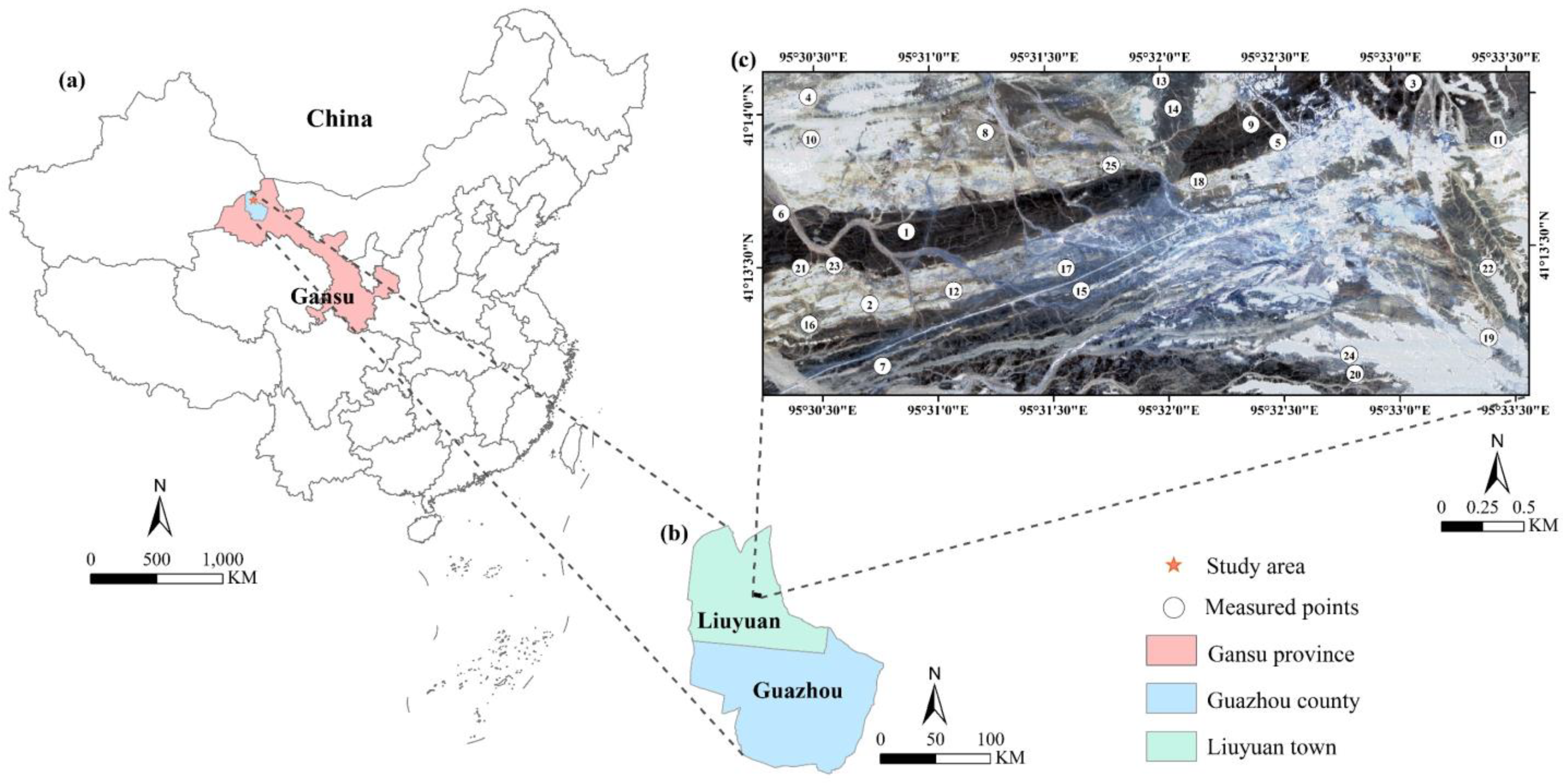
3.1. Overview of Study Site

The study area, located in northwestern Gansu, China (41°13′–41°14′N; 95°30′–95°33′E), is shown in Figure 1a,b. The area covers approximately 9.34 km² and has an altitude ranging from 1700 to 2000 m. This area exhibits an arid environment characterized by undulating Gobi terrain and a lack of vegetation but has excellent bedrock exposure [37]. The area is characterized by complex geological conditions and contains a major ore-forming zone, making it an ideal location for obtaining high-quality TIR hyperspectral images.

3.2. TASI Data and Pre-Processing

TASI is equipped with 32 channels within the 8–11.5 µm range. The sensor operated at a 2 km altitude, capturing the image in September 2010. The TASI data were provided by the Beijing Research Institute of Uranium Geology (Beijing, China). Pre-processing of the TIR hyperspectral image involves radiometric calibration, atmospheric correction, and temperature emissivity separation [38]. Radiometric calibration was processed with the system software provided by Canada ITRES operated by the Beijing Research Institute of Uranium Geology (Beijing, China). Atmospheric correction and temperature emissivity separation were implemented using MATLAB R2019a. An atmospheric radiation transfer model with intermediate spectral resolution was used for atmospheric correction to correct atmospheric absorption and upwelling radiation [38]. The image processed in the previous step was transformed into emissivity and temperature images using the normalized emissivity module (NEM), the emissivity ratio module (RATIO), and the average/maximum-minimum difference module (MMD) [39]. Channels having wavelengths greater than 11 µm and less than 8.5 µm were removed to ensure the accuracy of inversion because some are in non-atmospheric windows and subject to environmental influences. Finally, 22 channels were chosen, ranging from channel 6 to channel 27. Figure 1c depicts the color composite hyperspectral emissivity image.

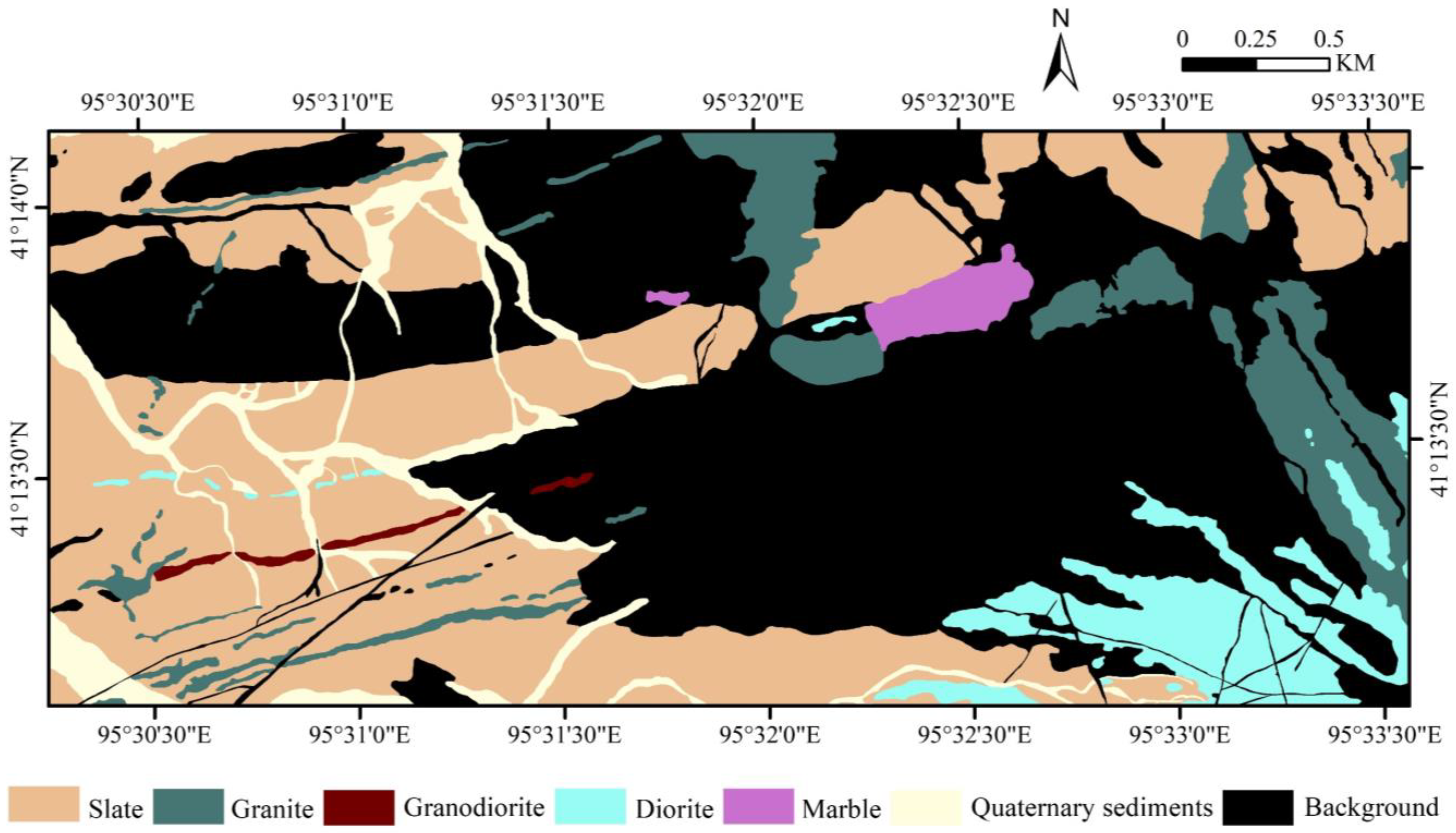
3.3. Geological Background and Ground-Truth Data

Tectonically, the study area lies within the Yujingzi and Liuyuan intracontinental rift zones on the southern margin of the Beishan epicontinental active belt, situated between the Tarim and Sino-Korean plates [40]. The region exhibits complex geological conditions with exposed strata [41]. The study area features slate, granite, granodiorite, diorite, marble, and quaternary sediments. To obtain precise geological information, a combination of outdoor field surveys and indoor laboratory analyses was conducted. Outdoor activities were carried out in late August 2020, including Global Positioning System (GPS) surveys and rock collection. Indoor rock thermal infrared spectra measurements were conducted using the 102F portable Fourier transform infrared spectrometer (FTIR). Ground-truth data involved 25 points with GPS coordinates, rock-type details, and thermal infrared spectra. As shown in Figure 1c, slate is represented by points 1 to 12, granite by points 13 to 16, granodiorite by point 17, diorite by points 18 to 24, and marble by point 25. Figure 2 shows several hand specimen images and several field photographs. Most studies use geological maps as reference maps. Since geological maps are only a general description of the geological situation, while remote sensing images reflect the real surface, geological maps lack pixel-by-pixel verifiability. In this case, we interpreted the TASI image based on geological resources [9,41] and the lithological types of the ground-truth data, as shown in Figure 3, facilitating algorithm evaluation.

4. Methodology

A schematic diagram illustrating the methodology adopted in this study is presented in Figure 4, which consists of four processes. The first part is the input of pre-processed surface emissivity TASI data. The second part involves constructing a sample dataset from the emissivity data using MLS3. This dataset is divided into training, validation, and test sets for the next part. The third part involves training, validating, and testing the dataset obtained in the previous step using different DL models. To validate the performance, each model is run five times. The best-performing model from these runs is selected for the next part. The fourth part involves generating the lithological map using the best model. The two main processes, “sample dataset construction” and “lithological map creation models”, will be described in detail.

These methods were implemented in ENVI 5.3.1 on a Windows 10 computer with an Intel i7-10700K CPU and 16 GB of RAM, as well as in Python 3.8 on a machine equipped with an Intel Xeon Silver 4210R, 20 GB of RAM, and a NVIDIA GeForce RTX 3090.

4.1. Sample Dataset Construction

MLS3 is implemented to generate a sample dataset consisting of the following steps: multiple spectra extraction, spectra combination and optimization, lithological type identification, and sample selection, as shown in Figure 5.

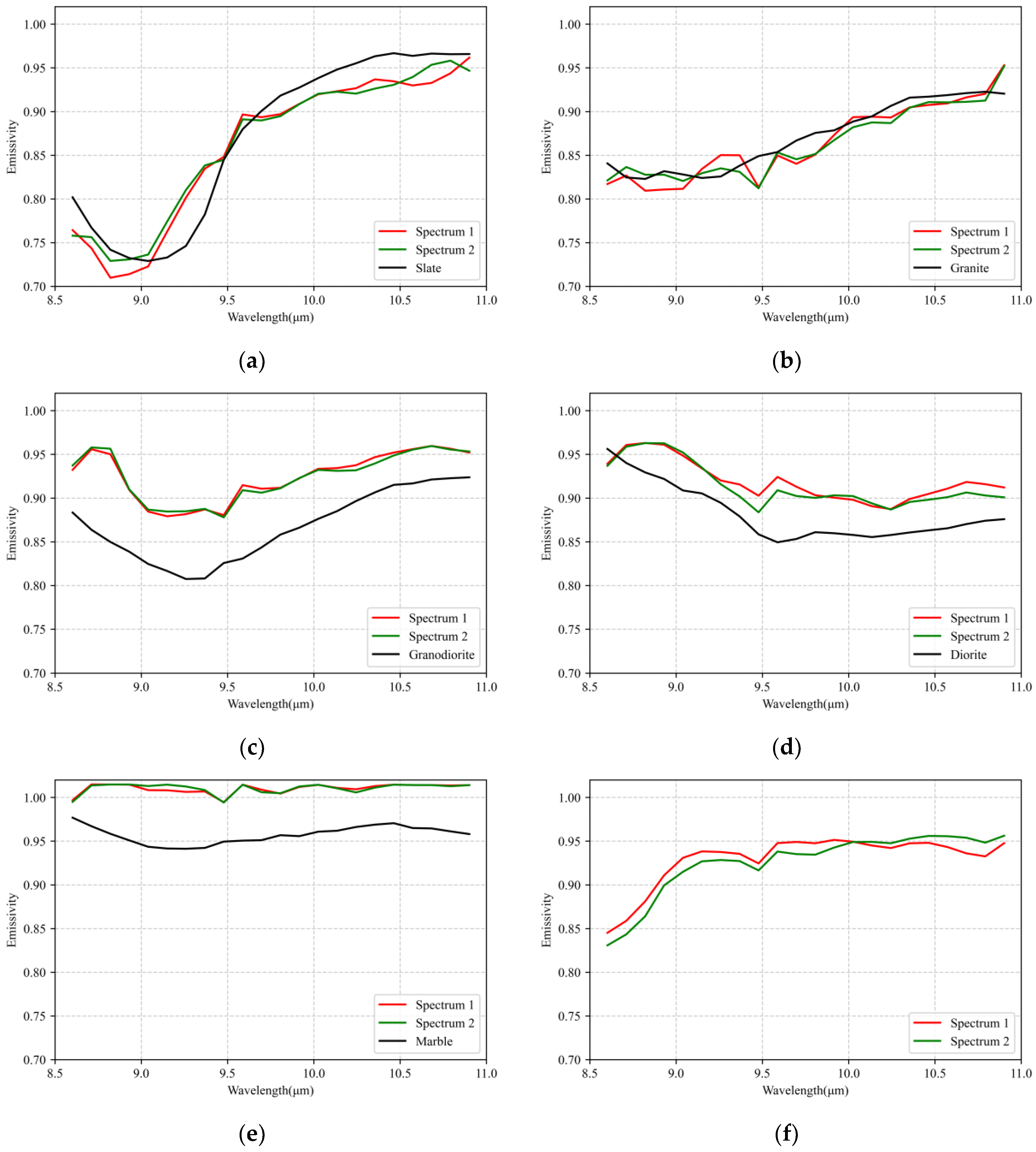
4.1.1. Multiple Spectra Extraction

In general, the same lithological type in remote sensing images may exhibit different states at different locations due to imaging conditions, resulting in variations or significant differences in the spectra of the same lithological type [42]. To overcome this effect, the original image is segmented into multiple patches based on its size to extract lithological endmember spectra. After segmentation, the image patches are significantly smaller than the original image. This processing helps extract richer lithological endmember spectral information, alleviates the problem of local spectral variability, and reduces the extraction errors of the lithological endmember spectra [42]. The number of lithological endmember spectra in each patch is determined using the hyperspectral signal subspace identification by minimum error (HySime) algorithm. The HySime algorithm, which estimates the dimensionality of hyperspectral subspaces, first calculates the correlation matrix of the signal and noise. It then selects the subspace with the smallest mean squared difference before and after projection in a space consisting of signal eigenvectors [43]. Bioucas-Dias and Nascimento [43] asserted that the number of endmembers is related to the subspace of eigenvectors that best captures the information in the original data. Therefore, the dimension of the eigenvector subspace is equal to the number of endmembers. Then, the lithological endmember spectra in each image patch can be extracted using the sequential maximum angle convex cone (SMACC) algorithm. SMACC, which is based on a convex cone model, identifies the lithological endmember spectra with the aid of constraints [44]. It uses the poles to identify the convex cone and define the first lithological endmember spectrum. The next lithological endmember spectrum is then generated by applying an oblique projection with constraints to the existing cone. Continue adding cones to generate new lithological endmember spectra. Repeat this process until the existing lithological endmember spectra are included in the generated convex cone or until a specified number of lithological endmember spectra classes are satisfied [44].

4.1.2. Spectra Combination and Optimization

After extracting the lithological endmember spectra from each image patch, all the lithological endmember spectra are collected into a set. K-means, which is an unsupervised learning algorithm [45], is used to cluster these spectra into different classes. After classifying the lithological endmember spectra, a single lithological type may correspond to multiple endmember spectra. When a large number of endmember spectra exist within a class, it increases the variety and quantity of endmember spectra but results in redundant calculations. In this case, the endmember average root mean square error (EAR) metric is employed to optimize the selection of lithological endmember spectra [46,47]. For a class with n lithological endmember spectra $\left\{{\mathrm{E}}_1,{\mathrm{E}}_2,...,{\mathrm{E}}_n\right\}$, the EAR for the ith lithological endmember spectrum is defined as follows:

$${\mathrm{EAR}}_i={\displaystyle \frac{1}{n-1}}\sum _{j=1}^n\mathrm{RMSE}({\mathrm{E}}_i,{\mathrm{E}}_j)$$

(1)

where ${\mathrm{E}\mathrm{A}\mathrm{R}}_i$ denotes the EAR for the ith lithological endmember spectrum. $\mathrm{RMSE}({\mathrm{E}}_i,{\mathrm{E}}_j)$ represents the average root mean square error between ${\mathrm{E}}_i$ and ${\mathrm{E}}_j$. A lower EAR value indicates a higher representativeness of the lithological endmember spectra. For each lithology, several representative spectra are chosen based on their EAR values.

4.1.3. Lithological Type Identification

After selecting the representative lithological endmember spectra, the spectral angle (SA) is utilized to classify these spectra. SA considers that a smaller spectral angle indicates a closer similarity between the representative lithological endmember spectra and the measured lithological spectra [48]. Consequently, the type of representative lithological endmember spectra is identified based on their best match to the measured lithological spectra. This method determines the type of representative lithological endmember spectra. The algorithm is both convenient and efficient and has been widely used for identifying lithological types [16,49]. The technique is implemented by applying:

$$\mathrm{S}\mathrm{A}={\cos }^{-1}\left({\displaystyle \frac{\overrightarrow{t}\cdot \overrightarrow{r}}{|\overrightarrow{t}|\cdot |\overrightarrow{t}|}}\right)$$

(2)

where SA is the spectral angle (in radians; 0 to 2$\pi$), t is the lithological endmember spectrum, and r is the measured lithological spectrum.

4.1.4. Sample Selection

After determining the types of all representative lithological endmember spectra, fully constrained linear spectral unmixing (FCLS) is used for sample selection, as follows:

$$x={\sum }_{i=1}^b{c}_i{e}_i+a$$

(3)

where b represents the total number of representative lithological endmember spectra. c_i denotes the abundance value corresponding to the ith representative lithological endmember spectrum e_i. a is an error term. x is any k dimensional spectral vector from the image (k is the number of bands in the image). Two constraints must be observed with FCLS: ${\sum }_{i=1}^b{c}_i=1$ and $0\le c_i\le 1$ [50,51].

All representative lithological endmember spectra are put into Equation (3) to generate the abundance map. Each pixel in the abundance map has a value ranging from 0 to 1. A pixel’s value closer to 1 indicates a higher likelihood that the pixel belongs to the type represented by that abundance map. The probability that a pixel belongs to a specific class can be determined by a threshold. The sample selection method using the abundance map involves the following main steps: (1) The threshold is defined using histogram calculations. Specifically, the cumulative percentage of the histogram is calculated, and the threshold is set at the pixel value where this percentage exceeds a predefined value T. (2) Pixels are classified using the threshold. If a pixel’s abundance value exceeds the predefined value, it is assigned to a specific class. Otherwise, it is categorized as unclassified. (3) Since multiple representative lithological endmember spectra correspond to a single class, samples of the same class are grouped accordingly in steps (1) and (2) to generate a final labeled sample map. The pseudo-code of the algorithm is provided in Algorithm 1.

Algorithm 1 The sample selection using the abundance map

Input: Abundance map U (m, h, b), User defined given T

thresholds = []

# Compute the cumulative pixel percentage of the histogram and determine thresholds.

For band in range(b):

histogram, bins = np.histogram(U[:, :, band].flatten(), bins = 255)

cumulative_pixel_percentage = np.cumsum((histogram/np.sum(histogram) * 100))

indexes = np.argmax(cumulative_pixel_percentage >= T)

thresholds.append(bins[indexes])

end for

# Pixels in U that are greater than or equal to the thresholds in each band are marked with the band index, otherwise they are marked as 0.

outputs_list = []

For band in range(b):

outputs_list.append((U[:, :, band:band+1] >= thresholds[band]) * (band + 1))

end for

Sband = np.concatenate(outputs_list, axis = −1)

# Combine pixels belonging to the same lithological type and obtain a labeled map for each lithological type. Next, show an example of the code to get Sclass1.

Sclass-1 = np.sum(Sband[:, :, i:i + map_width], axis = −1, keepdims = True) # i denotes the starting band in the Sband that belongs to a particular lithological type; map_width denotes how many bands in total belong to this lithological type.

Sclass1 [Sclass1 != 0] = Label # Label indicates the value of the type.

# Obtain the labeled map.

S = np.dstack((Sclass1, Sclass2, …, Sclassq)) # q indicates the number of lithological types.

# Remove multi-class pixels and reduce ambiguity.

multiple_values = np.sum(S != 0, axis = −1) > 1

S[multiple_values] = 0

S = np.sum(S, axis = −1)

Output: Labeled sample map S (m, h)

4.2. Lithological Map Creation Models

The samples obtained using MLS3 are employed to evaluate five distinct DL models, including 2D-CNN [38], HybridSN [52], MSRN [53], SSRN [54], and SPRN [55]. To assess the applicability of the original network for lithological mapping, the structural integrity of the original network framework is maintained as much as possible. The networks are implemented using PyTorch 1.7, with a training epoch set at 300. An initial learning rate of 0.001 is established, which is reduced by a factor of 0.1 at the 100th epoch and by 0.01 at the 250th epoch. The Adam optimizer is utilized for training updates. Additionally, the batch size is set to 128, and the input image size is 7 × 7, eliminating the requirement for dimensionality reduction in the original data. A brief conceptual framework for the implemented DLs is presented below.

• Two-dimensional convolutional neural network (2D-CNN)

The 2D-CNN is a neural network designed for spatial feature extraction [38]. Firstly, convolutional layers are utilized to capture features such as edges and textures from the input data. Subsequently, pooling layers are used to reduce computational complexity and resource consumption. Finally, fully connected layers perform classification based on the features learned by the convolutional and pooling layers.

2.

Hybrid spectral CNN (HybridSN)

HybridSN is a CNN that integrates the features of both 2D-CNN and the three-dimensional convolutional neural network (3D-CNN) [52]. The 3D-CNN component is utilized to extract both spectral and spatial features from input data, while the 2D-CNN component enhances the learning and refinement of these abstract spatial features. Although 3D-CNN is effective in feature extraction, it involves significant computational complexity. The incorporation of 2D-CNN helps to reduce this complexity.

3.

Multiscale residual network (MSRN)

MSRN considers multi-scale feature extraction to capture optimal spatial features. Specifically, MSRN replaces depth separable convolution (DSC) with mixed depth convolution (MDConv) to extract features at different scales from each feature map [53]. This improves the feature representation capability of the network by considering feature interactions at different scales. MSRN replaces the convolutional layer in the conventional residual block with MDSConv and uses the multiscale residual block (MRB) as its main unit. The entire MSRN network consists of four MRB units. To further enhance feature representation capability, skip connections are incorporated into two cascaded MRBs. The maximum pooling layer is removed, and only the first two MRB blocks are retained due to the smaller input patch and the large amount of input data in this research.

4.

Spectral-spatial residual network (SSRN)

SSRN employs residual learning to construct spectral and spatial residual blocks [54]. Specifically, 3D convolutional layers are the fundamental elements, and a batch normalization layer is introduced after each convolutional layer to standardize the learning process and improve model performance. Each spectral residual block utilizes multiple 1 × 1 × k convolutional layers to extract and reduce the dimensionality of spectral features from the original input image. Each spatial residual block uses multiple 3 × 3 × 1 convolutional layers to learn and enhance spatial features.

5.

Spectral partitioning residual network (SPRN)

SPRN utilizes group convolution (GC) to partition the input spectra into multiple non-overlapping continuous sub-bands and employs cascaded parallel residual blocks to extract local spectral and spatial features from these sub-bands [55]. Simultaneously, ordinary convolution is utilized to extract global information over the entire band through additional branches. Finally, the input information, local information, and global information are fused through a skip connection.

5. Results

5.1. Sample Dataset Generation

Based on the procedure outlined in Section 4.1, a sample dataset was constructed.

Firstly, the TASI image was divided into six patches according to the size of the image. The HySime algorithm was then used to determine the number of lithological endmember spectra for each block. To ensure the inclusion of all crucial and significant spectra, eight lithological endmember spectra were extracted from each patch, totaling 48 spectra.

Secondly, these spectra were classified into six classes using the K-means algorithm. Two representative lithological endmember spectra were selected from each class using the EAR algorithm, considering the complexity of the geological conditions in the study area.

Thirdly, the measured infrared spectra were resampled to match the TASI bands, and these spectra were used to determine the type of representative lithological endmember spectra. The six sets of spectral curves are shown in Figure 6. Specifically, the first set of spectra corresponds to slate, exhibiting a spectral signature of quartz with a minimum emission near 9 µm, as illustrated in Figure 6a. The second set of spectra represents granite, displaying a broad emission signature in the 8.5–10 µm range, as shown in Figure 6b. The third set of spectra corresponds to granodiorite, as depicted in Figure 6c, exhibiting a distinct emission feature between 9 and 9.5 µm. The fourth set of spectra corresponds to diorite, as shown in Figure 6d, with a minimal emission near 9.5 µm. The fifth group of spectra is similar to marble, as shown in Figure 6e, and the marble spectrum is generally smooth without obvious spectral features. As shown in Figure 6f, the sixth set of spectra does not have a direct match with the measured TIR spectra. A brief mapping of the TASI data using the spectra reveals that the sixth set of spectra corresponds to the quaternary sediments in the image.

Fourth, the abundance maps were generated using FCLS. Then, these maps were processed to produce the initial labeled samples. In this process, the given value was set to 99.6%, which enables more accurate samples to be obtained. These initial samples can be further corrected and optimized according to the ground-truth data. In particular, if labeled samples are present in and around the measured data, the results are retained. Conversely, the initial results are supplemented. Figure 7 shows the identified samples using MLS3.

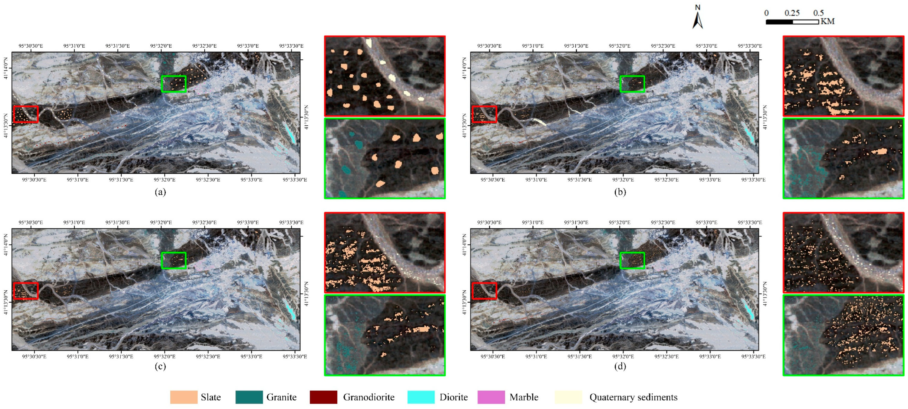
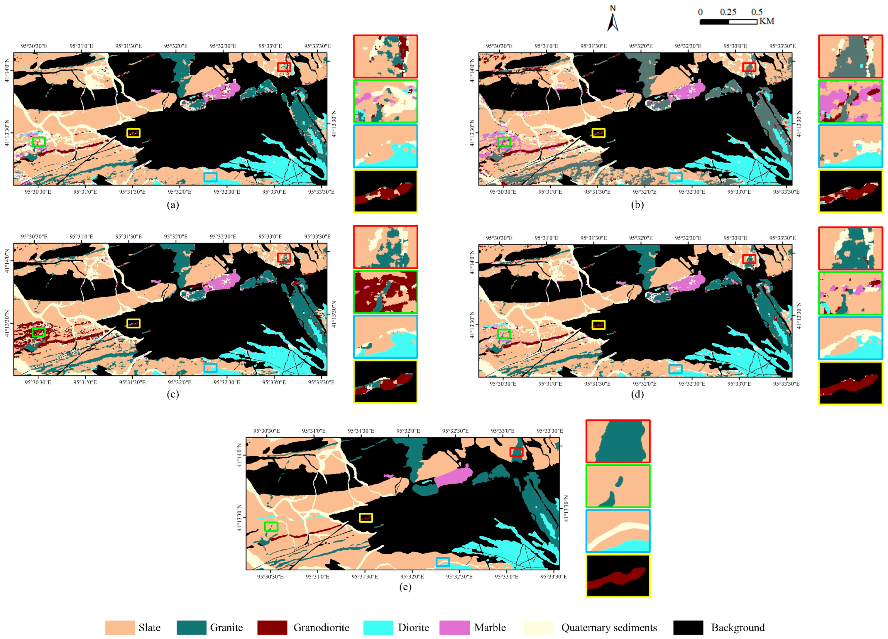
5.2. Lithological Mapping Results of DLs

These samples were divided into a training set, a validation set, and a test set in the ratio of 6:2:2, as shown in

Table 1. Sample dataset for the study area.

Lithologies	Training Set	Validation Set	Test Set
Slate	2676	892	893
Granite	1909	636	637
Granodiorite	409	136	138
Diorite	1734	578	579
Marble	303	101	101
Quaternary sediments	1077	359	360
Total	8108	2702	2708

. The performance of lithological map creation models is evaluated using overall accuracy (OA), user’s accuracy (UA), producer’s accuracy (PA), and kappa coefficient (Kappa).

Figure 8 shows the mapped results obtained from different DL algorithms. To highlight these differences, four locally enlarged patches, indicated by distinct colors (red, green, blue, and yellow), are situated on the right side of each image. Visually, the 2D-CNN algorithm demonstrates the most significant deviation between its results and the reference map. This discrepancy arises from its constitutive structure, which includes only two convolutional layers designated for feature extraction. Due to this limitation, the feature extraction capabilities of the algorithm are curtailed, resulting in a high volume of misidentifications. HybridSN performs closer to the reference image compared to 2D-CNN because HybridSN considers both the spatial and spectral features of lithology. MSRN, SSRN, and SPRN, particularly the SPRN algorithm, demonstrate clearer lithological boundaries and superior results compared to those of 2D-CNN and HybridSN. SPRN outperforms other methods by reducing the input dimension of each CNN and by fusing local spectral features with global features to obtain more accurate semantic information. Therefore, SPRN contributes to superior performance and delivers the most accurate result.

Table 2. Mapped results of different DL methods.

Lithologies	2D-CNN		HybridSN		MSRN		SSRN		SPRN
	PA	UA	PA	UA	PA	UA	PA	UA	PA	UA
Slate	67.56	89.86	72.21	92.22	76.92	93.51	83.28	93.70	83.25	95.27
Granite	65.70	74.41	75.46	63.56	78.35	71.12	75.34	81.58	79.17	82.98
Granodiorite	57.35	18.92	63.67	19.03	81.31	24.01	80.15	31.51	93.68	31.65
Diorite	78.54	66.93	77.08	83.68	83.06	86.75	89.91	90.44	94.43	87.90
Marble	73.98	22.38	77.51	39.08	81.26	42.24	85.79	50.60	84.98	58.39
Quaternary sediments	74.56	38.63	77.85	43.51	80.76	49.15	82.49	52.22	84.77	54.19
OA	69.14		73.81		78.27		82.69		84.03
Kappa	0.5331		0.5947		0.6573		0.7179		0.7416

provides the mapping accuracy of various algorithms. Quantitatively, compared to 2D-CNN, HybridSN, MSRN, and SSRN, SPRN performs notably better, exhibiting superior OA values higher by 14.89%, 10.22%, 5.76%, and 1.34%, respectively. This improvement is further reflected in the Kappa values, with Kappa values higher by 0.2085, 0.1469, 0.0843, and 0.0237, respectively. In the slate type, both the PA and UA of SSRN and SPRN are higher than those of the other algorithms. Notably, the UA of SPRN outperforms all other algorithms at 95.27%. For categories such as granite, granodiorite, and quaternary sediments, SPRN demonstrates significantly superior PA and UA results compared to those of the other methods. In the diorite type, SPRN surpasses other algorithms with a PA value of 94.43%. As for the marble type, SPRN leads with a UA value of 58.39%. Therefore, SPRN consistently delivers higher mapping accuracy due to its robust feature extraction capability.

5.3. Comparison of Sample Collection Methods

To demonstrate the effectiveness of the MLS3 method described in this paper for lithological mapping, we conducted a comparative analysis with three representative sample collection methods.

• ROI: ROI selects patches from the image as samples based on user selection.
• Spectral angle mapping (SAM): SAM determines the samples by comparing the angle between the ground-measured spectra (used as the reference spectra) and the pixel spectra. Given that slate, granite, and diorite each have numerous field-measured spectra, selecting appropriate reference spectra becomes challenging. In our study, we have selected the measured spectra that exhibit the highest correlation with the image endmember spectra to ensure the greatest similarity between the reference spectra and the pixel spectra. Notably, the type of quaternary sediment lacks matching field-measured spectra, so its lithological endmember spectrum is used.
• Spectral unmixing (SU): SU extracts one spectrum for each lithology and uses FCLS to generate abundance maps. It utilizes the abundance map to select samples for each class.

To ensure a fair comparison, the samples from ROI and MLS3 were selected to match in number, and their spatial distributions were made as similar as possible. Furthermore, the samples obtained through both SAM and SU methods underwent the same correction procedures based on ground-truth data.

Table 3. Sample size for different sample dataset construction methods.

Lithologies	ROI	SAM	SU	MLS3
Slate	4461	3502	4181	4461
Granite	3182	1794	4305	3182
Granodiorite	683	463	699	683
Diorite	2891	2413	2888	2891
Marble	505	131	539	505
Quaternary sediments	1796	3437	1743	1796
Total	13,518	11,740	14,355	13,518

effectively illustrates the number of samples obtained through various sample dataset construction methods. Table 3 shows that the total number of samples for these lithologies is approximately 13,000. Among the methods, SU procures the highest number of samples, while SAM yields the fewest. MLS3 and ROI obtain a moderate number of samples. For each lithology type, the number of samples collected by ROI, SU, and MLS3 is generally comparable, while SAM collects significantly fewer samples than the other methods. Figure 9 visually illustrates the spatial distribution of the samples obtained using different algorithms. To highlight the differences, two locally enlarged patches are provided on the right side of each image, indicated by distinct colors (red and green). Panels (a)–(d) of Figure 9 show the sample datasets obtained by ROI, SAM, SU, and MLS3, respectively. Subsequently, these samples were input into the SPRN classifier. The effectiveness of the sample dataset construction algorithms is evaluated based on the mapping accuracy achieved by SPRN.

Figure 10 presents the mapped results obtained using different sample acquisition methods. To highlight the differences, four zoomed-in patches are displayed on the right side of each map, distinguished by unique colors (red, green, blue, and yellow). As shown in Figure 10, the result generated by MLS3 demonstrates a closer alignment with the reference map, revealing more distinct lithological boundaries. In contrast, the results from ROI, SAM, and SU exhibit more misclassification and low spatial aggregation, indicating that the samples obtained through MLS3 are more representative and provide more accurate mapping results.

Table 4. Mapped results of different sample acquisition methods.

Lithologies	ROI		SAM		SU		MLS3
	PA	UA	PA	UA	PA	UA	PA	UA
Slate	83.64	92.33	73.70	94.45	79.01	94.61	83.25	95.27
Granite	72.14	82.77	82.79	64.96	78.74	74.76	79.17	82.98
Granodiorite	89.68	32.46	89.29	20.35	89.97	12.43	93.68	31.65
Diorite	94.16	84.11	95.28	85.86	92.28	90.25	94.43	87.90
Marble	71.02	54.10	79.19	38.56	82.15	66.60	84.98	58.39
Quaternary sediments	73.84	49.58	68.25	50.08	81.29	56.26	84.77	54.19
OA	81.78		77.07		80.70		84.03
Kappa	0.7003		0.6455		0.6946		0.7416

compares the mapping accuracies achieved by different sample dataset construction methods. It is evident from Table 4 that the MLS3 achieves a higher OA, with improvements of 2.25%, 6.96%, and 3.33% over ROI, SAM, and SU, respectively. Additionally, the MLS3 exhibits a superior Kappa, with improvements of 0.0413, 0.0961, and 0.047 compared to the aforementioned algorithms. For the slate and granite types, the UA values obtained by MLS3 are significantly higher than those obtained by those obtained by the other algorithms, suggesting that MLS3 rarely misclassifies other lithologies into these two lithologies. For the granodiorite type, diorite, marble, and quaternary sediments, the PA values garnered by MLS3 vastly surpass those of other algorithms, indicating that MLS3 rarely omits these lithologies. This underscores the exemplary results yielded by the sample dataset construction method we proposed.

6. Discussions

6.1. Sample Dataset Construction Algorithmic Considerations

Before implementing the lithological map creation algorithms, a large number of training samples need to be acquired [56,57]. The choice of spectra is essential throughout the entire MLS3. Hyperspectral image mapping typically uses ground truth or laboratory spectra as the reference spectra for lithological mapping [58]. However, environmental, climatic, and temporal factors can cause significant differences between ground-truth or laboratory spectra and image spectra. Furthermore, the phenomenon that there are variations in the spectra of the same class at different locations in the image cannot be avoided. To address these issues, various effective algorithms, such as SMACC, K-means, SA, EAR, and FCLS, are applied to help us select the most representative lithological endmember spectra, ensuring the chosen samples are appropriate for each class. During the process, the optimal number of lithological spectra and the given threshold for abundance image are the two primary factors. In general, the number of spectra required per class should be determined by the actual geological conditions. In this study, two spectra per class are sufficient for lithological identification. Moreover, the given threshold of 99.6% is appropriate as it ensures the quantity of samples while maintaining their quality.

In evaluating different methods for constructing sample datasets, it is evident that each approach has unique challenges and limitations. While the quantity of samples obtained through ROI matches that of MLS3, the ROI results are greatly susceptible to human influence. Different investigators may choose varying samples, potentially affecting the accuracy of lithological mapping. SAM obtains the smallest number of samples. Because SAM uses measured spectra to select samples, there may be inaccuracies in comparing these measured spectra to pixel spectra in the images, leading to unsatisfactory results. Even though SU obtains a larger number of samples than others, it overlooks the variability of lithologies across different regions and the variations in endmember spectra within the same class, leading to poor sample quality. In contrast, our proposed MLS3 method considers these factors. Although it generates fewer samples than SU, the quality of the samples is significantly higher. Consequently, MLS3 ensures both satisfactory sample quantity and quality.

Furthermore, the application of MLS3 requires geological knowledge of the study area to achieve more accurate lithological mapping results. The algorithms used in this study rely on geo-specific measurements, such as high-quality field spectral data, lithology types of field-measured points, and accurate GPS coordinates, to produce more reliable results. In situations where field data is unavailable, geological maps remain a plausible approach, providing insight into the local geological context.

6.2. DL Algorithmic Considerations

As for the lithological map creation models, five state-of-the-art CNN models were selected from the existing literature and tested using samples obtained from MLS3 based on the airborne TASI hyperspectral data. The experimental results indicate all models performed well, achieving good lithological mapping results. However, there is an imbalance in the UA accuracy values for each category obtained by these algorithms. For instance, SPRN has a UA of only 31.65% for granodiorite. The UA for marble and quaternary sediments hovers at around 55%, implying misidentification. One potential contributor to this discrepancy could be the class imbalance. Slate and granite are abundant throughout the study area, while granodiorite and marble appear in lesser quantities. This discrepancy may make it difficult for the algorithm to establish relationships between samples, leading to misidentification. Another aspect is the mineralogical similarity between certain lithologies, like granite and granodiorite. This resemblance can lead to instances of granites being incorrectly classified as granodiorite. Therefore, in the future, efforts should be made to optimize the training process of the models and change the learning strategy [59] to improve the performance of CNNs. Or try to use other types of neural network models, such as graph convolutional network (GCN) [60], transformer [61], etc. In addition, the combination of multi-source data has been shown to improve the accuracy of lithological mapping, so using data from multiple sources could be explored in the future.

7. Conclusions

This study explores the practical challenges encountered in leveraging DL for generating lithological maps. These challenges include the difficulty in acquiring representative samples arising from inadequate verifiability, subjective bias, and differences in the spectra of the same class at different locations in the hyperspectral image. We evaluated the efficacy of the proposed MLS3 and tested the abilities of different DL models utilizing TASI data gathered from the Liuyuan area in Gansu Province, China. Based on both theoretical and empirical results, we draw the following conclusions:

(1)

MLS3 considers the potential differences in spectra of the same lithology, reduces the influence of subjective factors, and achieves an overall accuracy of 2.25–6.96% higher than other sample collection methods. In general, MLS3 is designed to generate labeled samples in a more scientific and comprehensive manner.

(2)

MLS3 can be successfully applied to various DL models to enhance the performance of lithological mapping. Particularly, SPRN shows the best result compared to other CNN methods, with 84.03% for OA and 0.7416 for Kappa, respectively. SPRN improves the lithological mapping task due to its strong learning capabilities.

The above results show excellent mapping accuracy, providing some solution ideas for lithological mapping when using DL models but lacking samples. However, improving the accuracy of lithological mapping remains a challenging task. In future work, more complex DL models and multi-resource remote sensing data will be tried for experimental applications and evaluations.

References

1. El Fels, A.E.A.; El Ghorfi, M. Using Remote Sensing Data for Geological Mapping in Semi-Arid Environment: A Machine Learning Approach. Earth Sci. Inform. 2022, 15, 485–496. [Google Scholar] [CrossRef]
2. Han, W.; Zhang, X.; Wang, Y.; Wang, L.; Huang, X.; Li, J.; Wang, S.; Chen, W.; Li, X.; Feng, R.; et al. A Survey of Machine Learning and Deep Learning in Remote Sensing of Geological Environment: Challenges, Advances, and Opportunities. ISPRS J. Photogramm. Remote Sens. 2023, 202, 87–113. [Google Scholar] [CrossRef]
3. Shirmard, H.; Farahbakhsh, E.; Muller, R.D.; Chandra, R. A Review of Machine Learning in Processing Remote Sensing Data for Mineral Exploration. Remote Sens. Environ. 2022, 268, 112750. [Google Scholar] [CrossRef]
4. Hosseinjani, M.; Tangestani, M.H. Mapping Alteration Minerals Using Sub-Pixel Unmixing of ASTER Data in the Sarduiyeh Area, SE Kerman, Iran. Int. J. Digit. Earth 2011, 4, 487–504. [Google Scholar] [CrossRef]
5. Kodikara, G.R.L.; Woldai, T. Spectral Indices Derived, Non-Parametric Decision Tree Classification Approach to Lithological Mapping in the Lake Magadi Area, Kenya. Int. J. Digit. Earth 2018, 11, 1020–1038. [Google Scholar] [CrossRef]
6. Peyghambari, S.; Zhang, Y. Hyperspectral Remote Sensing in Lithological Mapping, Mineral Exploration, and Environmental Geology: An Updated Review. J. Appl. Remote Sens. 2021, 15, 031501. [Google Scholar] [CrossRef]
7. Tripathi, M.K.; Govil, H.; Chattoraj, S.L. Identification of Hydrothermal Altered/Weathered and Clay Minerals through Airborne AVIRIS-NG Hyperspectral Data in Jahajpur, India. Heliyon 2020, 6, e03487. [Google Scholar] [CrossRef] [PubMed]
8. Raj, S.K.; Ahmed, S.A.; Srivatsav, S.K.; Gupta, P.K. Iron Oxides Mapping from E0-1 Hyperion Data. J. Geol. Soc. India 2015, 86, 717–725. [Google Scholar] [CrossRef]
9. Ye, B.; Tian, S.; Cheng, Q.; Ge, Y. Application of Lithological Mapping Based on Advanced Hyperspectral Imager (AHSI) Imagery Onboard Gaofen-5 (GF-5) Satellite. Remote Sens. 2020, 12, 3990. [Google Scholar] [CrossRef]
10. Shirmard, H.; Farahbakhsh, E.; Heidari, E.; Beiranvand Pour, A.; Pradhan, B.; Müller, D.; Chandra, R. A Comparative Study of Convolutional Neural Networks and Conventional Machine Learning Models for Lithological Mapping Using Remote Sensing Data. Remote Sens. 2022, 14, 819. [Google Scholar] [CrossRef]
11. van der Meer, F.D.; van der Werff, H.M.A.; van Ruitenbeek, F.J.A.; Hecker, C.A.; Bakker, W.H.; Noomen, M.F.; van der Meijde, M.; Carranza, E.J.M.; de Smeth, J.B.; Woldai, T. Multi- and Hyperspectral Geologic Remote Sensing: A Review. Int. J. Appl. Earth Obs. Geoinf. 2012, 14, 112–128. [Google Scholar] [CrossRef]
12. Raji, O.; Ouabid, M.; Bodinier, J.-L.; El Messbahi, H.; Malainine, C.E.; Tabbakh, Z. An Integrated Approach for Rapid Delineation of K-Rich Syenites Suitable as Unconventional Potash Resources. Nat. Resour. Res. 2021, 30, 3219–3239. [Google Scholar] [CrossRef]
13. Zheng, S.; An, Y.; Shi, P.; Zhao, T. Mapping the Lithological Features and Ore-Controlling Structures Related to Ni-Cu Mineralization in the Eastern Tian Shan, NW China from ASTER Data. Remote Sens. 2021, 13, 206. [Google Scholar] [CrossRef]
14. Ni, L.; Xu, H.; Zhou, X. Mineral Identification and Mapping by Synthesis of Hyperspectral VNIR/SWIR and Multispectral TIR Remotely Sensed Data with Different Classifiers. IEEE J. Sel. Top. Appl. Earth Obs. Remote Sens. 2020, 13, 3155–3163. [Google Scholar] [CrossRef]
15. Aslett, Z.; Taranik, J.V.; Riley, D.N. Mapping Rock Forming Minerals at Boundary Canyon, Death Valey National Park, California, Using Aerial SEBASS Thermal Infrared Hyperspectral Image Data. Int. J. Appl. Earth Obs. Geoinf. 2018, 64, 326–339. [Google Scholar] [CrossRef]
16. Black, M.; Riley, T.R.; Ferrier, G.; Fleming, A.H.; Fretwell, P.T. Automated Lithological Mapping Using Airborne Hyperspectral Thermal Infrared Data: A Case Study from Anchorage Island, Antarctica. Remote Sens. Environ. 2016, 176, 225–241. [Google Scholar] [CrossRef]
17. Cui, J.; Yan, B.; Dong, X.; Zhang, S.; Zhang, J.; Tian, F.; Wang, R. Temperature and Emissivity Separation and Mineral Mapping Based on Airborne TASI Hyperspectral Thermal Infrared Data. Int. J. Appl. Earth Obs. Geoinf. 2015, 40, 19–28. [Google Scholar] [CrossRef]
18. Chen, Y.; Dong, Y.; Wang, Y.; Zhang, F.; Liu, G.; Sun, P. Machine Learning Algorithms for Lithological Mapping Using Sentinel-2 and SRTM DEM in Highly Vegetated Areas. Front. Ecol. Evol. 2023, 11, 1250971. [Google Scholar] [CrossRef]
19. Xi, J.; Jiang, Q.; Liu, H.; Gao, X. Lithological Mapping Research Based on Feature Selection Model of ReliefF-RF. Appl. Sci. 2023, 13, 11225. [Google Scholar] [CrossRef]
20. Kumar, C.; Chatterjee, S.; Oommen, T.; Guha, A. Automated Lithological Mapping by Integrating Spectral Enhancement Techniques and Machine Learning Algorithms Using AVIRIS-NG Hyperspectral Data in Gold-Bearing Granite-Greenstone Rocks in Hutti, India. Int. J. Appl. Earth Obs. Geoinf. 2020, 86, 102006. [Google Scholar] [CrossRef]
21. Othman, A.A.; Gloaguen, R. Integration of Spectral, Spatial and Morphometric Data into Lithological Mapping: A Comparison of Different Machine Learning Algorithms in the Kurdistan Region, NE Iraq. J. Asian Earth Sci. 2017, 146, 90–102. [Google Scholar] [CrossRef]
22. Wang, X.; Zuo, R.; Wang, Z. Lithological Mapping Using a Convolutional Neural Network Based on Stream Sediment Geochemical Survey Data. Nat. Resour. Res. 2022, 31, 2397–2412. [Google Scholar] [CrossRef]
23. Yu, J.; Zhang, L.; Li, Q.; Li, Y.; Huang, W.; Sun, Z.; Ma, Y.; He, P. 3D Autoencoder Algorithm for Lithological Mapping Using ZY-1 02D Hyperspectral Imagery: A Case Study of Liuyuan Region. J. Appl. Remote Sens. 2021, 15, 042610. [Google Scholar] [CrossRef]
24. Pan, T.; Zuo, R.; Wang, Z. Geological Mapping via Convolutional Neural Network Based on Remote Sensing and Geochemical Survey Data in Vegetation Coverage Areas. IEEE J. Sel. Top. Appl. Earth Obs. Remote Sens. 2023, 16, 3485–3494. [Google Scholar] [CrossRef]
25. Wang, Z.; Zuo, R.; Liu, H. Lithological Mapping Based on Fully Convolutional Network and Multi-Source Geological Data. Remote Sens. 2021, 13, 4860. [Google Scholar] [CrossRef]
26. Han, W.; Li, J.; Wang, S.; Zhang, X.; Dong, Y.; Fan, R.; Zhang, X.; Wang, L. Geological Remote Sensing Interpretation Using Deep Learning Feature and an Adaptive Multisource Data Fusion Network. IEEE Trans. Geosci. Remote Sens. 2022, 60, 1–14. [Google Scholar] [CrossRef]
27. Zhang, C.; Yi, M.; Ye, F.; Xu, Q.; Li, X.; Gan, Q. Application and Evaluation of Deep Neural Networks for Airborne Hyperspectral Remote Sensing Mineral Mapping: A Case Study of the Baiyanghe Uranium Deposit in Northwestern Xinjiang, China. Remote Sens. 2022, 14, 5122. [Google Scholar] [CrossRef]
28. Jia, S.; Jiang, S.; Lin, Z.; Li, N.; Xu, M.; Yu, S. A Survey: Deep Learning for Hyperspectral Image Classification with Few Labeled Samples. Neurocomputing 2021, 448, 179–204. [Google Scholar] [CrossRef]
29. Lin, C.; Guo, S.; Chen, J.; Sun, L.; Zheng, X.; Yang, Y.; Xiong, Y. Deep Learning Network Intensification for Preventing Noisy-Labeled Samples for Remote Sensing Classification. Remote Sens. 2021, 13, 1689. [Google Scholar] [CrossRef]
30. Dong, Y.; Yang, Z.; Liu, Q.; Zuo, R.; Wang, Z. Fusion of GaoFen-5 and Sentinel-2B Data for Lithological Mapping Using Vision Transformer Dynamic Graph Convolutional Network. Int. J. Appl. Earth Obs. Geoinf. 2024, 129, 103780. [Google Scholar] [CrossRef]
31. Cardoso-Fernandes, J.; Teodoro, A.C.; Lima, A.; Roda-Robles, E. Semi-Automatization of Support Vector Machines to Map Lithium (Li) Bearing Pegmatites. Remote Sens. 2020, 12, 2319. [Google Scholar] [CrossRef]
32. Serbouti, I.; Raji, M.; Hakdaoui, M.; El Kamel, F.; Pradhan, B.; Gite, S.; Alamri, A.; Maulud, K.N.A.; Dikshit, A. Improved Lithological Map of Large Complex Semi-Arid Regions Using Spectral and Textural Datasets within Google Earth Engine and Fused Machine Learning Multi-Classifiers. Remote Sens. 2022, 14, 5498. [Google Scholar] [CrossRef]
33. Abrams, M.; Yamaguchi, Y. Twenty Years of ASTER Contributions to Lithologic Mapping and Mineral Exploration. Remote Sens. 2019, 11, 1394. [Google Scholar] [CrossRef]
34. Clabaut, É.; Lemelin, M.; Germain, M.; Williamson, M.-C.; Brassard, É. A Deep Learning Approach to the Detection of Gossans in the Canadian Arctic. Remote Sens. 2020, 12, 3123. [Google Scholar] [CrossRef]
35. Pal, M.; Rasmussen, T.; Porwal, A. Optimized Lithological Mapping from Multispectral and Hyperspectral Remote Sensing Images Using Fused Multi-Classifiers. Remote Sens. 2020, 12, 177. [Google Scholar] [CrossRef]
36. Lin, N.; Fu, J.; Jiang, R.; Li, G.; Yang, Q. Lithological Classification by Hyperspectral Images Based on a Two-Layer XGBoost Model, Combined with a Greedy Algorithm. Remote Sens. 2023, 15, 3764. [Google Scholar] [CrossRef]
37. Li, C.; Tian, S.; Li, S.; Yin, M. Temperature and Emissivity Separation via Sparse Representation with Thermal Airborne Hyperspectral Imager Data. J. Appl. Remote Sens. 2016, 10, 042003. [Google Scholar] [CrossRef]
38. Liu, H.; Wu, K.; Xu, H.; Xu, Y. Lithology Classification Using TASI Thermal Infrared Hyperspectral Data with Convolutional Neural Networks. Remote Sens. 2021, 13, 3117. [Google Scholar] [CrossRef]
39. Gillespie, A.; Rokugawa, S.; Matsunaga, T.; Cothern, J.S.; Hook, S.; Kahle, A.B. A Temperature and Emissivity Separation Algorithm for Advanced Spaceborne Thermal Emission and Reflection Radiometer (ASTER) Images. IEEE Trans. Geosci. Remote Sens. 1998, 36, 1113–1126. [Google Scholar] [CrossRef]
40. Cui, J.; Yan, B.; Wang, R.; Tian, F.; Zhao, Y.; Liu, D.; Yang, S.; Shen, W. Regional-Scale Mineral Mapping Using ASTER VNIR/SWIR Data and Validation of Reflectance and Mineral Map Products Using Airborne Hyperspectral CASI/SASI Data. Int. J. Appl. Earth Obs. Geoinf. 2014, 33, 127–141. [Google Scholar] [CrossRef]
41. Wang, C.; Du, Z.; Yu, X.; Li, Y.; Lv, X.; Sun, H.; Du, Y. 1:50 000 Mineral Geological Map Database of the Huaniushan Map-Sheet, Gansu. Geol. China 2019, 46, 55–65. [Google Scholar] [CrossRef]
42. Li, H.; Wu, K.; Xu, Y. An Integrated Change Detection Method Based on Spectral Unmixing and the CNN for Hyperspectral Imagery. Remote Sens. 2022, 14, 2523. [Google Scholar] [CrossRef]
43. Bioucas-Dias, J.M.; Nascimento, J.M.P. Hyperspectral Subspace Identification. IEEE Trans. Geosci. Remote Sens. 2008, 46, 2435–2445. [Google Scholar] [CrossRef]
44. Gruninger, J.H.; Ratkowski, A.J.; Hoke, M.L. The Sequential Maximum Angle Convex Cone (SMACC) Endmember Model. In Proceedings of the Algorithms and Technologies for Multispectral, Hyperspectral, and Ultraspectral Imagery X, SPIE, Orlando, FL, USA, 12 August 2004; Volume 5425, pp. 1–14. [Google Scholar]
45. Jain, A.K.; Dubes, R.C. Algorithms for Clustering Data; Prentice-Hall, Inc.: Upper Saddle River, NJ, USA, 1988; ISBN 978-0-13-022278-7. [Google Scholar]
46. Dennison, P.E.; Roberts, D.A. Endmember Selection for Multiple Endmember Spectral Mixture Analysis Using Endmember Average RMSE. Remote Sens. Environ. 2003, 87, 123–135. [Google Scholar] [CrossRef]
47. Quintano, C.; Fernández-Manso, A.; Roberts, D.A. Multiple Endmember Spectral Mixture Analysis (MESMA) to Map Burn Severity Levels from Landsat Images in Mediterranean Countries. Remote Sens. Environ. 2013, 136, 76–88. [Google Scholar] [CrossRef]
48. Kruse, F.A.; Lefkoff, A.B.; Boardman, J.W.; Heidebrecht, K.B.; Shapiro, A.T.; Barloon, P.J.; Goetz, A.F.H. The Spectral Image Processing System (SIPS)—Interactive Visualization and Analysis of Imaging Spectrometer Data. Remote Sens. Environ. 1993, 44, 145–163. [Google Scholar] [CrossRef]
49. Jain, R.; Sharma, R.U. Airborne Hyperspectral Data for Mineral Mapping in Southeastern Rajasthan, India. Int. J. Appl. Earth Obs. Geoinf. 2019, 81, 137–145. [Google Scholar] [CrossRef]
50. Heinz, D.; Chang, C.-I.; Althouse, M.L.G. Fully Constrained Least-Squares Based Linear Unmixing. In Proceedings of the IEEE 1999 International Geoscience and Remote Sensing Symposium. IGARSS’99 (Cat. No.99CH36293), Hamburg, Germany, 28 June –2 July 1999; Volume 2, pp. 1401–1403. [Google Scholar]
51. Heylen, R.; Burazerovic, D.; Scheunders, P. Fully Constrained Least Squares Spectral Unmixing by Simplex Projection. IEEE Trans. Geosci. Remote Sens. 2011, 49, 4112–4122. [Google Scholar] [CrossRef]
52. Roy, S.K.; Krishna, G.; Dubey, S.R.; Chaudhuri, B.B. HybridSN: Exploring 3-D–2-D CNN Feature Hierarchy for Hyperspectral Image Classification. IEEE Geosci. Remote Sens. Lett. 2020, 17, 277–281. [Google Scholar] [CrossRef]
53. Gao, H.; Yang, Y.; Li, C.; Gao, L.; Zhang, B. Multiscale Residual Network with Mixed Depthwise Convolution for Hyperspectral Image Classification. IEEE Trans. Geosci. Remote Sens. 2021, 59, 3396–3408. [Google Scholar] [CrossRef]
54. Zhong, Z.; Li, J.; Luo, Z.; Chapman, M. Spectral-Spatial Residual Network for Hyperspectral Image Classification: A 3-D Deep Learning Framework. IEEE Trans. Geosci. Remote Sens. 2018, 56, 847–858. [Google Scholar] [CrossRef]
55. Zhang, X.; Shang, S.; Tang, X.; Feng, J.; Jiao, L. Spectral Partitioning Residual Network with Spatial Attention Mechanism for Hyperspectral Image Classification. IEEE Trans. Geosci. Remote Sens. 2022, 60, 1–14. [Google Scholar] [CrossRef]
56. He, X.; Chen, Y. Transferring CNN Ensemble for Hyperspectral Image Classification. IEEE Geosci. Remote. Sens. Lett. 2021, 18, 876–880. [Google Scholar] [CrossRef]
57. Masarczyk, W.; Głomb, P.; Grabowski, B.; Ostaszewski, M. Effective Training of Deep Convolutional Neural Networks for Hyperspectral Image Classification through Artificial Labeling. Remote Sens. 2020, 12, 2653. [Google Scholar] [CrossRef]
58. Kale, K.V.; Solankar, M.M.; Nalawade, D.B.; Dhumal, R.K.; Gite, H.R. A Research Review on Hyperspectral Data Processing and Analysis Algorithms. Proc. Natl. Acad. Sci. India Sect. A Phys. Sci. 2017, 87, 541–555. [Google Scholar] [CrossRef]
59. Paoletti, M.E.; Haut, J.M.; Plaza, J.; Plaza, A. Deep Learning Classifiers for Hyperspectral Imaging: A Review. ISPRS J. Photogramm. Remote Sens. 2019, 158, 279–317. [Google Scholar] [CrossRef]
60. Yu, L.; Peng, J.; Chen, N.; Sun, W.; Du, Q. Two-Branch Deeper Graph Convolutional Network for Hyperspectral Image Classification. IEEE Trans. Geosci. Remote Sens. 2023, 61, 1–14. [Google Scholar] [CrossRef]
61. Ding:, K.; Lu, T.; Fu, W.; Li, S.; Ma, F. Global-Local Transformer Network for HSI and LiDAR Data Joint Classification. IEEE Trans. Geosci. Remote Sens. 2022, 60, 1–13. [Google Scholar] [CrossRef]
Figure 1. Map of study area locations: (a) Guazhou County within Gansu Province, China; (b) study area in Liuyuan Town, Guazhou County; (c) color composite hyperspectral image and measured points in the field.
Remotesensing 16 02852 g001
Figure 2. Hand specimen images and field photographs. (ad) Hand specimen images. These hand specimens were obtained from points 12, 15, 19, and 21, respectively; (e,f) Field photographs. These field photographs were taken at points 14 and 15, respectively.
Remotesensing 16 02852 g002
Figure 3. Annotation map of the study area (according to [9,41] and ground-truth information from Figure 1c modification).
Remotesensing 16 02852 g003
Figure 4. Workflow of the experimental process in this paper.
Remotesensing 16 02852 g004
Figure 5. Overview of MLS3 for sample dataset construction.
Remotesensing 16 02852 g005
Figure 6. Six groups extracted lithological spectra (red and green lines) and their closest match from the field spectra data (black line): (a) matching results for the first group of spectra; (b) matching results for the second group of spectra; (c) matching results for the third group of spectra; (d) matching results for the fourth group of spectra; (e) matching results for the fifth group of spectra; (f) the sixth group of extracted lithological spectra.
Remotesensing 16 02852 g006
Figure 7. Sample distribution map of the study area.
Remotesensing 16 02852 g007
Figure 8. Resultant maps of different DL methods: (a) 2D-CNN; (b) HybridSN; (c) MSRN; (d) SSRN; (e) SPRN; (f) reference image.
Remotesensing 16 02852 g008
Figure 9. Samples selected using different sample acquisition methods: (a) ROI; (b) SAM; (c) SU; (d) MLS3.
Remotesensing 16 02852 g009
Figure 10. Resultant maps of different sample dataset construction methods: (a) ROI; (b) SAM; (c) SU; (d) MLS3; (e) reference image.
Remotesensing 16 02852 g010