Multi-Stage Frequency Attention Network for Progressive Optical Remote Sensing Cloud Removal

Abstract

Cloud contamination significantly impairs optical remote sensing images (RSIs), reducing their utility for Earth observation. The traditional cloud removal techniques, often reliant on deep learning, generally aim for holistic image reconstruction, which may inadvertently alter the intrinsic qualities of cloud-free areas, leading to image distortions. To address this issue, we propose a multi-stage frequency attention network (MFCRNet), a progressive paradigm for optical RSI cloud removal. MFCRNet hierarchically deploys frequency cloud removal modules (FCRMs) to refine the cloud edges while preserving the original characteristics of the non-cloud regions in the frequency domain. Specifically, the FCRM begins with a frequency attention block (FAB) that transforms the features into the frequency domain, enhancing the differentiation between cloud-covered and cloud-free regions. Moreover, a non-local attention block (NAB) is employed to augment and disseminate contextual information effectively. Furthermore, we introduce a collaborative loss function that amalgamates semantic, boundary, and frequency-domain information. The experimental results on the RICE1, RICE2, and T-Cloud datasets demonstrate that MFCRNet surpasses the contemporary models, achieving superior performance in terms of mean absolute error (MAE), root mean square error (RMSE), peak signal-to-noise ratio (PSNR), and structural similarity index (SSIM), validating its efficacy regarding the cloud removal from optical RSIs.

1. Introduction

Remote sensing technology serves as an indispensable tool, enabling the continuous and swift acquisition of geometric and physical information pertaining to Earth’s surface [1]. Accompanying the rapid advancements in remote sensing technologies, optical RSIs have emerged as the predominant medium for Earth observation [2]. Nonetheless, the presence of clouds, which envelop approximately 55% of Earth’s surface, markedly hinders the interpretation and utility of optical RSIs [3]. Consequently, cloud removal from optical RSIs presents a significant challenge [4].

The traditional cloud removal techniques primarily rely on the principle of local correlation among adjacent pixels, predicated on the assumption that cloud-covered areas possess similar characteristics to their adjacent cloud-free regions [5]. As a result, these techniques utilize the data from cloud-free regions to reconstruct or substitute the cloud-covered areas, employing methods such as interpolation [6], filtering [7], and exemplar-based strategies [8], among others. Zhu et al. [9] introduced a novel cloud removal approach utilizing a modified neighborhood similar pixel interpolator (NSPI). Similarly, Siravenha et al. [10] employed a high boost filter alongside homomorphic filtering for scattered cloud elimination, while He et al. [11] proposed an innovative image completion technique through the analysis of similar patch offsets. These methods fundamentally assume a resemblance in the features between cloud-covered and cloud-free areas. Nonetheless, they might introduce discontinuities or artifacts at the boundaries of the newly generated cloud-free areas and the original cloud-covered regions, leading to unnatural effects in the restored images [12]. Moreover, these approaches often require manual parameter adjustments to achieve optimal results, adding complexity and potentially resulting in inconsistent performances [13].

The advent of machine learning techniques, including decision trees (DTs) [14], support vector machines (SVMs) [15], random forests (RFs) [16], and others, has significantly mitigated the constraints of the conventional cloud removal methods. By leveraging extensive datasets comprising both cloudy and cloud-free imagery, machine learning models adeptly discern intricate patterns and distinctions between these regions. Consequently, they possess the capability to distinguish between the cloudy and cloud-free areas in images, facilitating effective cloud restoration. Lee et al. [17] introduced multicategory support vector machine (MSVM) as a promising, efficient algorithm for cloud removal preprocessing. Hu et al. [18] developed a thin cloud removal algorithm for contaminated RSIs, combining multidirectional dual-tree complex wavelet transform (M-DTCWT) with domain adaptation transfer least square support vector regression (T-LSSVR), ensuring the preservation of the ground object details while eliminating thin clouds. Tahsin et al. [19] devised an innovative optical cloud pixel recovery (OCPR) method using an RF trained on multi-parameter hydrological data to restore the cloudy pixels in Landsat NDVI imagery. However, machine learning approaches typically do not directly derive high-level feature representations from raw data. Instead, they depend on the expertise and prior knowledge of domain experts for feature selection. The effectiveness of image reconstruction is profoundly influenced by the quality and selection of these handcrafted features, introducing a degree of subjectivity and inherent limitations.

The recent integration of deep learning’s robust nonlinear modeling capabilities, particularly through convolutional neural networks (CNNs), has revolutionized the cloud removal efforts. These networks can autonomously learn feature representations from raw data, eliminating the necessity for manual feature extraction or selection. This end-to-end learning paradigm significantly diminishes the need for manual input in cloud removal processes. Zhang et al. [20] introduced DeepGEE-S2CR, a method combining Google Earth Engine (GEE) data with a multi-level feature-connected CNN, to efficiently clear the clouds in Sentinel-2 imagery using Sentinel-1 synthetic aperture radar imagery as supplementary data. Meanwhile, Ma et al. [21] proposed the innovative cloud-enhancement GAN (Cloud-EGAN) strategy, which incorporates saliency and high-level feature enhancement modules within a cycle-consistent generative adversarial network (CycleGAN) framework. The widespread implementation of CNNs has significantly improved the cloud removal models’ ability to discern complex features and variations between the cloud-covered and cloud-free regions in images, leading to the enhanced reconstruction of cloudy imagery.

In traditional CNN architectures, the model’s effective receptive field is constrained by the network’s depth and the size of the convolutional kernels, limiting the ability to capture comprehensive features and contextual information [22]. This restriction hampers the model’s capacity to process global information from images. To overcome this limitation, attention mechanisms [23] have been integrated into cloud removal models to augment their capability to assimilate global information, enabling dynamic focus adjustment across different image regions. Such enhancements allow these models to prioritize the reconstruction of cloudy areas, thereby significantly improving their contribution to image analysis. Xu et al. [24] introduced AMGAN-CR, which effectively leverages attention maps alongside attentive recurrent and residual networks, coupled with a reconstruction network, to tackle the challenges of cloud removal. Wu et al. [25] proposed Cloudformer, a transformer-based model that integrates convolution and self-attention mechanisms with locally enhanced positional encoding (LePE), adeptly managing cloud removal by extracting features across various scales and augmenting the positional encoding capabilities.

Despite the promising results demonstrated by the existing deep learning cloud removal models, they still face significant limitations. Specifically, these models [26,27] primarily rely on a per-pixel approach during the training process, which neglects the global coherence between pixels. This leads to difficulties in seamlessly integrating the reconstructed regions with the surrounding cloud-free areas at the semantic level. To address this challenge, studies such as [28,29] have introduced mask techniques aimed at more accurately distinguishing cloud-covered areas from cloud-free regions, thereby guiding the detailed reconstruction of local features and transitions. However, the accuracy of these masks remains a critical factor limiting their performance. Additionally, the attention mechanisms currently employed in cloud removal tasks mainly focus on channel and spatial attention, largely overlooking the crucial role of the frequency features within the image [30]. Frequency features, as another important dimension of image information, are essential for capturing both the global structure and local details of an image. Therefore, effectively integrating frequency features into cloud removal models to achieve a unified reconstruction of the cloud-covered and cloud-free regions, thereby enhancing the quality and semantic consistency of the reconstructed images, remains a pressing research problem.

To address these problems, we introduce a frequency-domain attention mechanism utilizing the fast Fourier transform (FFT) to enhance the spatial information processing and performance of cloud removal models given that frequency information is critical for cloud removal. Low frequencies highlight the overall content of an image, while high frequencies focus on the edge contours and texture details. Leveraging high-frequency information is essential. Moreover, precise boundary delineation is vital in cloud removal to accurately identify cloud-covered regions, enabling targeted reconstruction efforts that preserve the integrity of cloud-free areas. We propose a multi-stage reconstruction strategy to refine the boundary features and design a collaborative optimization loss function to concentrate on the boundaries of cloud-covered areas while minimizing unnecessary reconstruction in cloud-free zones. The principal contributions are summarized as follows:

(1) We propose a frequency cloud removal module (FCRM) that is adept at recovering the details while preserving the original characteristics of non-cloud regions in the frequency domain. The FCRM utilizes frequency-domain attention to focus on the differences in the frequency-domain information between cloudy and cloud-free images to refine the boundary information of the image. Additionally, it introduces the non-local attention block to capture the local and non-local relationships and enhance the contextual connections through global dependency relationships.

(2) We introduce a collaborative optimization loss function, consisting of Charbonnier loss for global robustness, edge loss for edge-preserving precision, and FFT loss for frequency-aware adaptability, which penalize boundary shifts while ensuring subject consistency and retaining intricate image details and textures.

(3) The multi-stage frequency attention network (MFCRNet) is structured around an encoder–decoder architecture, specifically designed for reconstructing areas obscured by clouds. Utilizing FCRM modules in the preceding $N-1$ layers enables meticulous cloud removal from input images. To minimize the information loss from up-sampling operations, a variant ResNet is directly applied to the input image in the N-th layer.

(4) A series of experiments are conducted on the RICE1, RICE2 [31], and T-Cloud [32] datasets, demonstrating the feasibility and superiority of the proposed method. It exhibits superior performance in both the quantitative and qualitative assessments compared to the other cloud removal methods.

2. Related Work

2.1. Cloud Removal

This section introduces several techniques for removing clouds, which can be broadly classified into single-stage and multi-stage approaches based on their architectural designs.

2.1.1. Single-Stage Approach

Predominantly, cloud removal techniques employ a single-stage design, where the models directly learn the mapping from raw input data to the final output. For example, Bermudez et al. [33] used cloudless optical imaging areas and the corresponding synthetic aperture radar (SAR) data to train conditional generative hostile networks (CGans) to rely solely on SAR data to clear clouds. Meraner et al. [34] developed a deep residual neural network tailored for cloud removal tasks in SAR–optical fusion. Zhou et al. [35] created a cloud removal framework based on a generative adversarial network (GAN), which integrates coherent semantics and local adaptive reconstruction considerations. Feng et al. [36] utilized self-attention to capture global dependencies, proposing a method that incorporates global–local fusion for cloud removal. Nonetheless, single-stage cloud removal approaches often struggle to adequately extract and leverage the information from the input images, which may result in suboptimal outcomes, especially in complex cloud coverage scenarios. This limitation underscores the need for exploring alternative, more sophisticated methods that offer nuanced and adaptable solutions for cloud removal.

2.1.2. Multi-Stage Approach

Contrary to the single-stage approach, the multi-stage approach breaks down the cloud removal task into several phases, offering more precise control over the image cloud removal process. Zheng et al. [4] developed a two-stage methodology for the complex task of single-image cloud removal, utilizing a U-Net architecture for the thin cloud elimination in the initial stage and a GAN for the dense cloud removal in the later stage, acknowledging the distinct strategies required for different types of clouds. Jiang et al. [37] introduced a sophisticated network capable of dividing the cloud removal process into coarse and refined phases, thereby enabling a more thorough and detailed approach to the task. Darbaghshahi et al. [38] proposed a dual-stage GAN for converting SAR-to-optical images and for subsequent cloud removal. Similarly, Tao et al. [39] presented a two-stage strategy for sequential cloud-contaminated area reconstruction, focusing initially on global structure recovery and subsequently on enhancing the content details for a more nuanced restoration.

2.2. Attention Mechanisms

In traditional CNN models, each neuron is connected only to its immediate neighbors, restricting the model’s capacity to grasp long-range dependencies [40]. To address this limitation, the attention mechanism, inspired by human selective attention, has been introduced. It allows the model to dynamically compute a weight distribution at each processing step based on contextual information, thereby focusing selectively on the most pertinent segments of the input relevant to the task at hand [41]. This enhancement significantly improves the model’s ability to perceive long-range dependencies and has gained widespread application across the machine learning and artificial intelligence domains [42].

In the context of cloud removal, the adoption of attention mechanisms is similarly extensive. Li et al. [43] proposed a hierarchical spectral and structure-preserving fusion network (HS²P) utilizing a hierarchical fusion of optical RSIs with SAR data. This approach includes a channel attention mechanism and a collaborative optimization loss function. Jin et al. [44] introduced HyA-GAN, a novel deep learning model for cloud removal in RSIs that integrates channel and spatial attention mechanisms into a generative adversarial network. Wang et al. [45] developed a method that leverages SAR images as supplementary data, integrating spatial and channel attention mechanisms alongside gated convolutional layers to enhance the cloud removal from optical images. In our proposed model, frequency-domain attention is employed to discern the edge details in missing regions, proving advantageous for the cloud removal process.

2.3. Learning in Frequency Domain

The frequency domain is utilized to analyze signals or functions based on their frequency components. Recently, deep learning has been introduced to efficiently process various tasks by utilizing frequency-domain information [46]. Rao et al. [47] proposed the global filter network, a technique designed to learn the long-term spatial dependencies within the frequency domain, with a specific focus on improving image classification tasks. Yang et al. [48] introduced an unsupervised domain adaptation strategy that seeks to reduce the disparity between source and target distributions by exchanging low-frequency spectra in semantic segmentation tasks. Zhong et al. [49] embedded clique structures in super-resolution processes, utilizing the inverse discrete wavelet transform (IDWT) for resizing feature maps. Chen et al. [50] developed the frequency spectrum modulation tensor complement method and used the Fourier transform in the time dimension to execute the low-rank complement for each frequency component, especially in the context of cloud removal. Building on the success of these frequency-based approaches, our work employs the fast Fourier transform as an effective tool for modeling the frequency information in cloud removal tasks. This enables comprehensive learning of the edge details within cloud-covered regions, facilitating a more focused and precise restoration strategy.

3. Materials and Methods

This section presents the introduction of the proposed method MFCRNet for cloud removal in optical RSIs. Section 3.1 provides an overview of the overall architecture. Subsequently, Section 3.2, Section 3.3 and Section 3.4 describe detailed descriptions of each module within the architecture. Finally, Section 3.5 explores the loss function employed by the model.

3.1. Overview

In Figure 1, a comprehensive approach is illustrated for maximizing the utilization of contextual information in cloud removal tasks through the construction of a deep architectural framework in MFCRNet. The shallow feature extraction block (SFEB) in each stage of MFCRNet encompasses a convolutional layer combined with a channel attention mechanism, which plays a pivotal role in extracting fundamental features. The frequency attention block (FAB) and non-local attention block (NAB) at the preceding $N-1$ stages operate sequentially in both frequency and spatial domains, progressively refining the cloud removal process. In the N-th stage, a variant ResNet is designed to generate pixel-wise accurate estimates while preserving the fine details. Furthermore, to enhance the recovery of spectral and structural features from global information, a collaborative optimization loss function is devised for training purposes.

3.2. Multi-Stage Progressive Architecture

As depicted in Figure 1, following N stages of progressive cloud removal, we derive the ultimate output of MFCRNet. To provide a clearer method description, we designate the initial $N-1$ stages as the frequency-domain-based cloud removal modules (FCRMs), with the final layer termed as the variant ResNet cloud removal module (VCRM). The primary information flow can be succinctly expressed by the following equation:

$$F_{out}=VCRM(I,FCR{M}_{out}^{k-1})$$

(1)

$$\begin{array}{cc}\hfill FCR{M}_{out}^{k-1}& =FCR{M}^{k-1}(I,FCR{M}_{out}^{k-2})\hfill \\ \hfill & =FCR{M}^{k-1}(I,(...FCR{M}^2(I,FCR{M}_{out}^1)))\hfill \\ \hfill & =FCR{M}^{k-1}(I,(...FCR{M}^2(I,FCR{M}^1\left(I\right))))\hfill \end{array}$$

(2)

where I represents the input cloudy image, $F_{out}$ represents the final restored cloudless image, $VCRM$ means the operation of the final stage, $FCR{M}^k$ means the operation of the k-th stage, $FCR{M}_{out}^k$ represents the intermediate result output after the k-th FCRM module operation, while $k=1,2,...,N-1$ and N is the total number of the stage of MFCRNet. The result of each stage is progressively passed on to the next stage until reaching the N-th stage. The final output is the result of gradual cloud removal at all stages with high-resolution features while mitigating the effect of clouds on the image. Inspired by previous work [51], we used a long skip connection to efficiently capture more information.

3.3. Frequency Attention Block

As illustrated in Figure 2a, the structure of the FAB follows an encoder–decoder architecture with the following components. First, to fully extract both high- and low-frequency information from the input images and simultaneously capture long-term and short-term interactions, we introduce the residual FFT-Conv block in Figure 2b. In addition to a normal spatial residual stream comprising two 3 × 3 convolutional layers followed by ReLU activation, another channel-wise FFT stream is integrated to explain the global context in the frequency domain. Initially, the transformation from the spatial domain to the frequency domain begins with the computation of the $2D$ real FFT of the input features Z, which decomposes the input features into their constituent frequency components. Upon performing the FFT operation, the resulting frequency-domain representation comprises both real and imaginary components. To preserve all the information within these components, they are combined along the channel dimension. Subsequently, the concatenated frequency-domain tensor undergoes a series of transformations (a $3\times 3$ convolutional layer, ReLU activation, and a $3\times 3$ convolutional layer) to refine its feature representation. Finally, the inverse $2D$ real FFT is employed to convert the refined frequency-domain representation back into the spatial domain, which reconstructs the spatial structure of the image, incorporating the refined frequency-domain information to produce a final feature map. To strike a balance between efficiency and effectiveness in cloud removal, each encoder block and decoder block comprises three residual FFT-Conv blocks. Second, inspired by the FCANet [52], which combines the channel attention mechanism with the discrete cosine transform (DCT) cleverly to generate controllable frequency-domain components, the feature maps at U-Net skip connections are processed with the FCA. In FCA, the input feature $X\in R^{C\times H\times W}$ is divided into n partitions along the channel dimension. For each partition, a $2D$ discrete cosine transform (DCT) is applied:

$$F^i=2DDC{T}_{u_i,v_i}\left(X^i\right)=\sum _{h=0}^{H-1}\sum _{w=0}^{W-1}{X}_{h,w}^{i}cos\left({\displaystyle \frac{u_i\pi (2h+1)}{2H}}\right)cos\left({\displaystyle \frac{v_i\pi (2w+1)}{2W}}\right)$$

(3)

where $u\in \left\{0,1,...,H-1\right\}$, $v\in \left\{0,1,...,W-1\right\}$ are the frequency component $2D$ indices corresponding to $X^i$ and $F^i\in R^{{\displaystyle \frac{C}{n}}}$ is the ${\displaystyle \frac{C}{n}}$ dimensional corresponding to $X^i$. The whole multi-spectral channel attention framework can be written as

$$O_{FFT}=Sigmoid\left(fc\left(concat(F^0,F^1,...,F^{n-1})\right)\right)$$

(4)

By using FCA as the skip connection in U-Net, the frequency-based representations obtained provide complementary information to the spatial representations so that the model gains access to a richer and more diverse set of features, potentially enhancing its ability to capture complex patterns and structures in the input data.

3.4. Non-Local Attention Block

As depicted in Figure 1, the final step of the MFCR involves the utilization of the NAB to further refine the restoration results. The details of NAB are demonstrated in Figure 3. The NAB operates by taking the input cloud image I and the feature map $FABout$ generated by FAB as inputs. It computes attention maps on $FABout$ by utilizing a non-local block (NLB) [53] that considers both local and non-local relationships. These attention maps are then used to enhance the features of the input image I. By computing pairwise similarities between feature vectors at all spatial positions, the NAB identifies relevant contextual information from distant regions in the image, enhancing the discriminative power of the maps. The attention-enhanced features generated by the NAB are then forwarded to the next stage for additional processing.

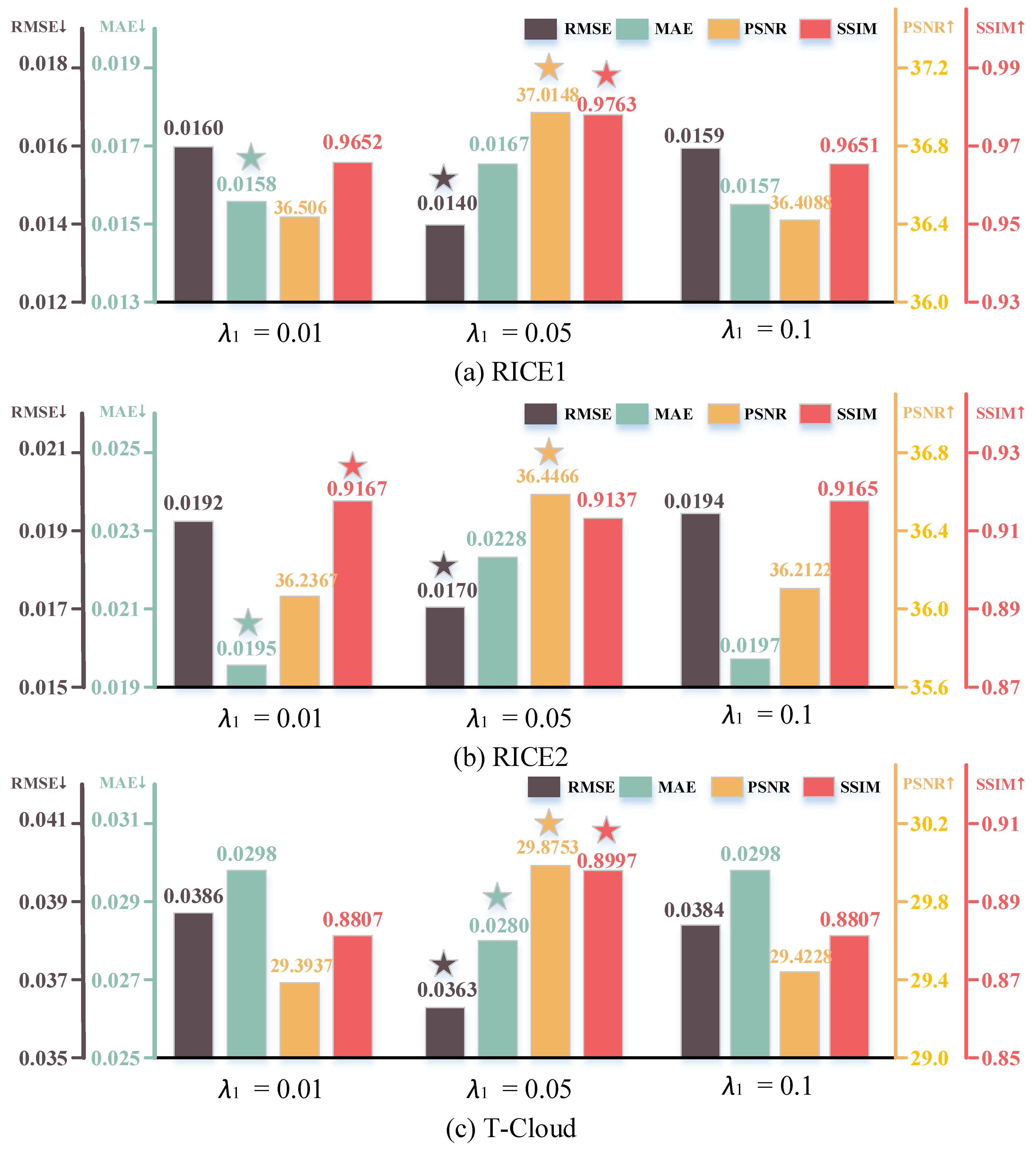
3.5. Collaborative Optimization Loss

In the current cloud removal tasks, the predominant utilization of the L2 loss function for content reconstruction often overlooks the importance of structural and global information. To address this limitation, we have devised a collaborative optimization loss function for training, which encompasses Charbonnier loss $L_c$ for global robustness, edge loss $L_e$ for edge-preserving precision, and FFT loss $L_f$ for frequency-aware adaptability. The collaborative optimization loss function is defined as

$$L=L_c+{\lambda }_1{L}_e+{\lambda }_2{L}_f$$

(5)

where ${\lambda }_1$ and ${\lambda }_2$ are the weights of the loss function, and we empirically set the values of these to 0.05 and 0.01, respectively.

By penalizing the discrepancy between predicted and ground truth pixel values using a robust L1 norm from global information, Charbonnier loss $L_c$ promotes the generation of restoration results that are less sensitive to outliers and exhibit greater resilience to noise. It is defined as

$$L_c=\sum _{n=0}^{n=N-1}\sqrt{{∥O_n-Y∥}^2+{\epsilon }^2}$$

(6)

where O means the final output of the MFCRNet, Y represents the ground-truth image, and $\epsilon$ is set to ${10}^{-3}$ empirically.

In order to preserve edge details and structural integrity within the restored images, ensuring that boundaries between cloud and non-cloud regions remain sharp and well-defined, the edge loss $L_e$ is designed to penalize deviations in edge locations and gradients between the predicted and ground truth images as

$$L_e=\sum _{n=0}^{n=N-1}\sqrt{{∥▵O_n-▵Y∥}^2+{\epsilon }^2}$$

(7)

where $▵$ means the Laplacian operator.

To encourage the model to faithfully reproduce both low- and high-frequency components, preserving the overall structure and texture of the scene, FFT loss $L_f$ leverages the frequency-domain representation of images to promote the restoration of global information and fine-grained structures, leading to more coherent and visually consistent outcomes, defined as

$$L_f=\sum _{n=0}^{n=N-1}{∥FT\left(O_n\right)-FT\left(Y\right)∥}_1$$

(8)

where $FT$ represents the FFT operation.

By combining Charbonnier loss $L_c$, edge loss $L_e$, and FFT loss $L_f$ into a unified collaborative optimization framework, our approach effectively addresses the shortcomings of traditional L2 loss-based methods by incorporating structural and global information into the training process. The collaborative optimization function ensures that the model learns to balance content fidelity, structural integrity, and global coherence, resulting in more accurate and visually pleasing cloud removal results.

4. Experiments

In this section, the dataset, evaluation metrics, and experimental setup are presented, followed by the experimental results and the ablation study.

4.1. Dataset

To thoroughly validate our proposed method’s effectiveness, we conducted experiments using the publicly available RICE and T-Cloud optical remote sensing datasets.

4.1.1. RICE Dataset

To thoroughly validate our proposed method’s effectiveness, we conducted experiments using the publicly available RICE optical remote sensing dataset. The RICE dataset has two subsets, namely RICE1 and RICE2, specifically designed for cloud removal tasks. The RICE1 dataset, sourced from Google Earth, includes 500 pairs of images: cloudy images and corresponding cloud-free images. The RICE2 dataset is derived from Landsat 8 OLI/TIRS and contains 736 sample pairs, each with cloudy images, cloud-free images, and corresponding cloud masks. The time difference between the images with clouds and their cloud-free counterparts does not exceed fifteen days. The size of the images in each dataset is $512\times 512$. For the RICE1 dataset, we partitioned 80% of the images, approximately 400, for training purposes, while the remaining 20% served as the test set. For the RICE2 dataset, we selected 589 images for training and 147 images for testing.

4.1.2. T-Cloud Dataset

The T-Cloud dataset is a large-scale dataset of 2939 pairs of real remotely sensed images captured by Landsat 8 satellites, and these image pairs demonstrate the contrast between thin cloud cover and its clear scene 16 days later, with diverse ground scenes, complex texture details, and challenging non-uniform cloud distributions. In our experiments, we follow an 8:2 ratio for the division, where the training set contains 2351 pairs of images, the test set contains 588 pairs of images, and the size of each image is $256\times 256$.

4.2. Evaluation Metrics

To quantify the quality of the final restored images, we employed commonly used evaluation metrics: peak signal-to-noise ratio (PSNR), structural similarity index (SSIM), mean absolute error (MAE), and root mean square error (RMSE). PSNR is a widely accepted metric for assessing the fidelity of the restored image against the ground truth image. SSIM measures the similarity between the restored and ground truth images concerning structure, luminance, and contrast. MAE evaluates the average magnitude of errors between the restored and ground truth images, providing a straightforward measure of the overall accuracy of the restoration process. RMSE calculates the square root of the mean squared differences between corresponding pixels of the restored and ground truth images taking into account both the magnitude and direction of the errors. It is worth noting that higher image quality is indicated by larger PSNR and SSIM values, as well as smaller MAE and RMSE values. The PSNR, SSIM, MAE, and RMSE are defined as follows:

$$SSIM(x,y)={\displaystyle \frac{(2{\mu }_x{\mu }_y+{\theta }_1)(2{\sigma }_{xy}+{\theta }_2)}{({\mu }_x+{\mu }_y+{\theta }_1)({\sigma }_x+{\sigma }_y+{\theta }_2)}}$$

(9)

$$MAE(x,y)={\displaystyle \frac{1}{H\times W}}\sum _{i=1}^H\sum _{j=1}^W\left|x(i,j)-y(i,j)\right|$$

(10)

$$RMSE(x,y)=\sqrt{{\displaystyle \frac{1}{H\times W}}\sum _{i=1}^H\sum _{j=1}^W{(x(i,j)-y(i,j))}^2}$$

(11)

$$PSNR(x,y)=20lo{g}_{10}\left({\displaystyle \frac{1}{RMSE(x,y)}}\right)$$

(12)

where x and y represent the two images being evaluated, and H and W, respectively, represent the height and width of the images. $(i,j)$ and $y(i,j)$ indicate the pixel values of the two images at pixel position $(i,j)$, respectively. ${\mu }_x$ and ${\mu }_y$ are the means of images x and y; ${\sigma }_x$ and ${\sigma }_y$ are the standard deviations of x and y, and y. ${\theta }_1$ and ${\theta }_2$ are constants.

4.3. Experimental Setup

We implemented the proposed method with the PyTorch framework on an NVIDIA A40 GPU. The Adam optimizer was employed to update the learnable parameters, with the exponential decay rates $\beta 1$ and $\beta 2$ set to 0.9 and 0.999, respectively. The $eps$ was set to $1\times {10}^{-8}$. The initial learning rate of the Adam optimizer was set to $2\times {10}^{-4}$, and then a cosine annealing strategy was used to dynamically update the learning rate. The training process ran for 250 epochs with a batch size of 4.

4.4. Comparison with Other Methods

In this section, we compare the proposed MFCRNet with five existing methods: Dark Channel Prior (DCP) [54], Pix2Pix [55], RCAN [56], SpAGAN [57], CVAE [32], and CMNet [58]. Among them, the DCP algorithm utilizes the characteristics of the dark channel in images and the physical model of fog to remove haze from images, representing a traditional approach based on a handcrafted prior. Both the Pix2Pix and SpAGAN methods are based on GAN models. Pix2Pix employs a conditional generative adversarial network to learn how to transform cloudy images into clear ones. SpAGAN integrates spatial attention mechanisms with generative adversarial networks to remove cloud from high-resolution satellite images. The RCAN method employs channel attention mechanisms and residual learning for cloud removal. The CVAE method generates multiple plausible cloud-free images using conditional variational autoencoders and addresses the cloud removal problem by analyzing uncertainty across multiple predictions. CMNet uses a cascaded memory network that combines local spatial detail extraction and global detail restoration.

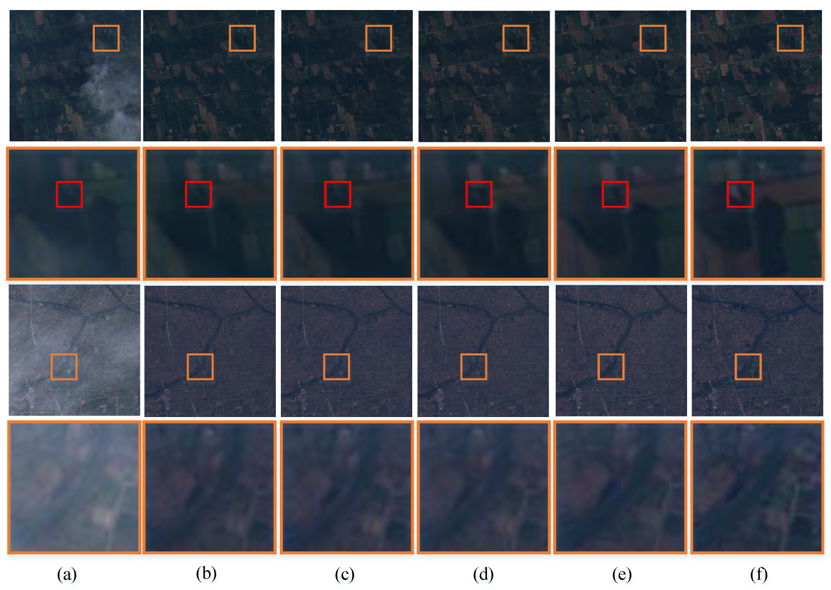
4.4.1. Results on RICE1 Dataset

Table 1. Quantitative results of different methods on RICE1 dataset, where ↓ means the higher score indicates the better effect, ↑ means the lower score indicates the better effect, and the bold text indicates the best results.

Method	$MAE(\downarrow )$	$RMSE(\downarrow )$	$PSNR(\uparrow )$	$SSIM(\uparrow )$
DCP	0.1402	0.1510	17.6752	0.8247
Pix2Pix	0.0679	0.0866	22.7856	0.8401
SpAGAN	0.0527	0.0557	27.7522	0.9608
RCAN	0.0279	0.0333	30.5608	0.9528
CVAE	0.0440	0.0520	27.2760	0.9632
CMNet	0.0213	0.0172	35.0473	0.9103
our MFCRNet	0.0140	0.0167	37.0148	0.9763

presents the quantitative experimental results of various methods on the RICE1 dataset, with the best results highlighted in bold. It is evident from the observations that each method’s performance across four evaluation metrics is distinct. Notably, our proposed MFCRNet method achieves ideal outcomes across all the evaluation metrics. Specifically, our method produces significant results on MAE/RMSE/PSNR/SSIM by 0.0140/0.0167/37.0148/0.9763. Compared to the other methods, the improvements on MAE/RMSE/PSNR/SSIM are at least by 0.0073/0.0005/1.9675/0.0131, underscoring the exceptional performance of our MFCRNet approach in cloud removal tasks.

Different methods’ cloud removal results on the RICE1 dataset are presented in Figure 4. In order to enhance the visual recognition and clarity, each selected area is clearly labeled by an orange box, and these areas are individually enlarged and subsequently arranged directly below the respective original image. We showcase the restoration outcomes for both greenery and mountainous regions. Our proposed approach not only performs excellently in terms of the local details and overall content preservation but also exhibits remarkable color fidelity. In the second and sixth rows of Figure 4, the results generated by the DCP (b) show severe image distortion, failing to accurately reproduce the color information of the ground scenes. This could be attributed to DCP’s primary focus on the dark channels containing high-brightness elements like sky and clouds, potentially leading to color distortion when removing these regions. Both Pix2Pix (c) and CVAE (f) yield subpar cloud removal results, exhibiting blurry effects. The spatial-attention-based SpAGAN (d) faces similar color distortion issues as DCP, possibly because it solely emphasizes local information while overlooking global contextual cues. On the other hand, RCAN (e) effectively alleviates the color distortion problem observed in SpAGAN by leveraging residual learning. However, despite achieving similar color tones as the reference cloud-free images, RCAN still exhibits some blurriness in certain edge regions. Although CMNet (g) demonstrates significant results in cloud removal, as shown in the second row, our method exhibits superior performance in restoring the clarity of the ground object contours, providing more accurate contour details. This is attributed to our utilization of the FAB for extracting detailed information such as image edges and the incorporation of NAB to enable the model to fully consider global dependencies, facilitating a comprehensive understanding of the image characteristics throughout the learning process.

4.4.2. Results on RICE2 Dataset

As shown in

Table 2. Quantitative results of different methods on RICE2 dataset, where the bold text indicates the best.

Method	$MAE(\downarrow )$	$RMSE(\downarrow )$	$PSNR(\uparrow )$	$SSTM(\uparrow )$
DCP	0.1455	0.1704	16.8548	0.5865
Pix2Pix	0.0563	0.0812	23.3966	0.6563
SpAGAN	0.0851	0.0958	27.0126	0.9030
RCAN	0.0942	0.1133	20.1369	0.7618
CVAE	0.0600	0.0770	25.2760	0.8009
CMNet	0.0248	0.0176	35.1383	0.8875
our MFCRNet	0.0170	0.0228	36.4466	0.9137

, the quantitative results of the various image restoration methods on the RICE2 dataset exhibit notable discrepancies across evaluation metrics such as MAE, RMSE, PSNR, and SSIM. Similar to the findings on the RICE1 dataset, our proposed method maintains excellent performance. These results underscore the substantial advantages of our MFCRNet method on the RICE2 dataset.

Figure 5 illustrates the results of the different methods for cloud removal on the RICE2 dataset. Compared to the RICE1 dataset, the RICE2 dataset exhibits higher density and thickness regarding the cloud images, which results in a significant loss of detailed information in the images. However, our method still optimally preserves the details and color information of the images. In the regions marked in the third and eighth rows of Figure 5, it is evident that the DCP (b) fails to effectively reconstruct the cloudy areas. This is attributed to the high brightness of the thick cloud regions compared to the underlying terrain, causing the pixel values in the dark channel to become overly saturated, thus hindering accurate cloud removal. In comparison to the traditional methods like DCP, Pix2Pix (c) based on deep learning shows improvement in cloud removal; however, difficulties persist in removing some clouds when the cloud coverage is extensive. Although the SpAGAN (d) achieves satisfactory cloud removal, noticeable differences in color distribution between the reconstructed results and ground truth are observed. The RCAN (e) fails to accurately reconstruct the edge features, resulting in blurred outlines of some terrain features. While the CVAE (f) can delineate terrain outlines more accurately, it tends to produce blurry results. It is obvious from the comparison in the sixth row that, when the cloud thickness reaches a level that almost obscures the ground objects, CMNet’s recovery appears to be suboptimal compared to our method, which demonstrates superior recovery when dealing with these types of extreme cloud cover situations. Our method fully utilizes contextual and boundary information, resulting in images with more restored details, fewer artifacts, and more realistic colors.

4.4.3. Results on T-Cloud Dataset

Table 3. Quantitative results of different methods on T-Cloud dataset, where the bold text indicates the best.

Method	$MAE(\downarrow )$	$RMSE(\downarrow )$	$PSNR(\uparrow )$	$SSTM(\uparrow )$
DCP	0.1139	0.0971	19.8694	0.0917
Pix2Pix	0.0735	0.0716	26.2355	0.6576
SpAGAN	0.0423	0.0419	26.6549	0.7159
RCAN	0.0851	0.0759	24.3434	0.6585
CVAE	0.0746	0.0728	24.0836	0.7941
CMNet	0.0390	0.0297	29.0990	0.7913
our MFCRNet	0.0363	0.0280	29.8753	0.8997

exhaustively compares the performance of MFCRNet with a variety of the existing methods on the T-Cloud dataset, demonstrating through quantitative evaluation that MFCRNet achieves the top results in all four key evaluation metrics. Further, Figure 6 visualizes the experimental results of MFCRNet regarding the qualitative analysis on the T-Cloud dataset and compares it with the other methods. Echoing the previous performances on the RICE1 and RICE2 datasets, MFCRNet once again proves its powerful ability: it can accurately recover the cloud-obscured regions while maintaining and enhancing the detailed information of the image during the recovery process, ensuring the overall quality of the image and the integrity of the information.

4.5. Effects of Different Stage Numbers

In the MFCRNet network, we further determined the number of stages N.

Table 4. Quantitative results of different stage numbers, where the bold text indicates the best.

Dataset	Stage	$MAE(\downarrow )$	$RMSE(\downarrow )$	$PSNR(\uparrow )$	$SSTM(\uparrow )$	Para (M)
	1	0.0162	0.0191	36.0252	0.9735	4.57
	2	0.0148	0.0176	36.7629	0.9753	6.37
RICE1	3	0.0144	0.0172	36.8485	0.9758	11.20
	4	0.0143	0.0170	36.8870	0.9759	16.04
	5	0.0140	0.0167	37.0148	0.9763	20.87
	6	0.0140	0.0168	37.0274	0.9761	25.71
	1	0.0190	0.0249	35.4552	0.9087	4.57
	2	0.0183	0.0242	35.9103	0.9117	6.37
RICE2	3	0.0181	0.0241	36.1480	0.9123	11.20
	4	0.0171	0.0226	36.4316	0.9134	16.04
	5	0.0170	0.0228	36.4466	0.9137	20.87
	6	0.0172	0.0230	36.4018	0.9136	25.71
	1	0.0392	0.0303	29.1369	0.8749	4.57
	2	0.0383	0.0297	29.4578	0.8820	6.37
T-Cloud	3	0.0381	0.0293	29.7754	0.8824	11.20
	4	0.0378	0.0297	29.8110	0.8904	16.04
	5	0.0363	0.0280	29.8753	0.8997	20.87
	6	0.0388	0.0302	29.2848	0.8848	25.71

shows the scores of the different evaluation metrics. For the RICE1 dataset, the network’s performance improves with the increase in the number of stages N until it reaches $N=$ 6. Although at $N=$ 6 the PSNR is 1.26% higher than at $N=$ 5, the other metrics do not perform as well as at $N=$ 5. Additionally, with the increasing number of layers, the model’s parameter count also increases. Therefore, we chose $N=$ 5 as a balance between the performance and parameter count.

4.6. Effects of Critical Module

To fully demonstrate the effectiveness of the proposed MFCRNet method, we conducted a series of ablation experiments to validate the contribution of each module comprising the MFCRNet method.

To illustrate the role of the FAB module in the MFCRNet architecture, in the fourth stage, we generated heatmaps from the input feature maps to the FAB module and the output feature maps from the FAB module, which are shown in Figure 7. From the second column, it is evident that, without passing through the FAB module, the extracted contours appear blurry. However, from the third column, it can be observed that, after passing through the FAB module, we can extract clearer contours. This comparison verifies that our FAB module, by transforming the spatial domain into the frequency domain and leveraging both low-frequency and high-frequency information, improves the quality of the image contours and enhances the representation of the key features.

In addition, we also conducted ablation experiments to quantitatively evaluate the contributions of the proposed modules on the RICE1, RICE2, and T-Cloud datasets. We set the baseline as using the U-Net network for the feature extraction and regular convolutional modules for the feature reconstruction. These results are shown in

Table 5. Ablation study on different modules in MFCRNet, where the bold text indicates the best.

Dataset	Module			$MAE(\downarrow )$	$RMSE(\downarrow )$	$PSNR(\uparrow )$	$SSTM(\uparrow )$
	Baseline	FAB	NAB
	✓	×	×	0.0155	0.0187	36.0884	0.9746
RICE1	✓	×	✓	0.0150	0.0183	36.2673	0.9744
	✓	✓	×	0.0149	0.0176	36.8983	0.9754
	✓	✓	✓	0.0140	0.0167	37.0148	0.9763
	✓	×	×	0.0173	0.0235	35.7890	0.9091
RICE2	✓	×	✓	0.0176	0.0236	35.8661	0.9099
	✓	✓	×	0.0172	0.0232	36.4391	0.9126
	✓	✓	✓	0.0170	0.0228	36.4466	0.9137
	✓	×	×	0.0373	0.0295	29.5268	0.8036
T-Cloud	✓	×	✓	0.0367	0.0291	29.5521	0.8367
	✓	✓	×	0.0382	0.0295	29.4303	0.8208
	✓	✓	✓	0.0363	0.0280	29.8753	0.8997

. It is evident that, when removing the FAB or NAB module, the performance metrics of the model decrease. The visualization results of the ablation experiments for each key module conducted on the datasets are shown in Figure 8, Figure 9 and Figure 10. From the highlighted areas, it is evident that our proposed method exhibits smooth and natural handling of the object edges, whereas the other methods appear blurry, demonstrating the effectiveness of our approach in improving the reconstruction quality.

4.7. Effects of Different Loss Functions

To verify the importance of the loss function in our work, we conducted ablation experiments on two datasets, employing different loss functions. As Charbonnier loss $L_c$ is commonly used in cloud removal tasks, we adopted it as our baseline, gradually adding boundary loss Le and frequency-domain loss $L_f$.

Table 6. Ablation study on different components of the loss functions in MFCRNet, where the bold text indicates the best.

Dataset	Module			$MAE(\downarrow )$	$RMSE(\downarrow )$	$PSNR(\uparrow )$	$SSTM(\uparrow )$
	${\mathbf{L}}_{\mathbf{c}}$	${\mathbf{L}}_{\mathbf{e}}$	${\mathbf{L}}_{\mathbf{f}}$
	✓	×	×	0.0153	0.0181	36.5095	0.9749
RICE1	✓	×	✓	0.0152	0.0179	36.6615	0.9750
	✓	✓	×	0.0142	0.0169	36.9770	0.9763
	✓	✓	✓	0.0140	0.0167	37.0148	0.9763
	✓	×	×	0.0173	0.0233	36.2906	0.9188
RICE2	✓	×	✓	0.0169	0.0229	36.3693	0.9119
	✓	✓	×	0.0166	0.0229	36.3726	0.9128
	✓	✓	✓	0.0170	0.0228	36.4466	0.9137
	✓	×	×	0.0412	0.0319	28.7120	0.8658
T-Cloud	✓	×	✓	0.0388	0.0299	29.1978	0.8071
	✓	✓	×	0.0415	0.0321	28.6515	0.7917
	✓	✓	✓	0.0363	0.0280	29.8753	0.8997

presents the quantitative results. We observed that using only $L_c$ led to the lowest evaluation scores. Introducing either $L_e$ or $L_f$ individually resulted in positive effects, while incorporating both $L_e$ and $L_f$ simultaneously maximized all the evaluation metrics. This indicates that our proposed loss functions facilitate the network to effectively learn more features during training, thereby being more beneficial for recovering detailed information. The visualization results of the ablation experiments for each loss function conducted on the datasets are shown in Figure 11, Figure 12 and Figure 13. We can see from the places marked with red boxes in Figure 12 that the (b) and (c) images without $L_f$ loss recover a part of the green swamp in the input image as a lake, which is not obscured by clouds in the input image, and thus the $L_f$ loss minimizes the unnecessary reconstruction of the cloud-free regions.

In addition, we paid special attention to the critical impact of the weighting parameters ${\lambda }_1$ and ${\lambda }_2$ on the experimental results. To this end, we carefully designed and executed a series of parameter sensitivity experiments. First, we kept the parameter ${\lambda }_2$ unchanged while setting the value of ${\lambda }_1$ to 0.01, 0.05, and 0.1 in turn, and tested them on three different datasets. By comparing the results of the experiments from Figure 14, we observed a clear trend: when ${\lambda }_1$ was set to 0.05, the model demonstrated optimal performance regarding all the metrics. Immediately thereafter, we fixed ${\lambda }_1$ at the optimal value identified above and turned to explore the effect of ${\lambda }_2$ on the model performance. Similarly, we set three test values for ${\lambda }_1$: 0.01, 0.05, and 0.1, and conducted experiments on the same dataset. As shown in Figure 15, we found that the model reached its best performance when ${\lambda }_1$ = 0.01. Combining the above experimental results, we determined the optimal combination of the weighting parameters ${\lambda }_1$ and ${\lambda }_2$ as ${\lambda }_1$ = 0.05 and ${\lambda }_2$ = 0.01.

5. Conclusions

In this study, we introduce a novel cloud removal network, leveraging a multi-stage frequency-domain attention mechanism designed to reconstruct the obscured information in optical images affected by cloud coverage. This framework progressively restores image detail by hierarchically deploying FCRMs. In the FCRM, the FAB aims to provide more distinguishable feature vectors between the cloud-covered and cloud-free regions, and the NAB is designed to propagate informative context to the next stage. Additionally, we employ a collaborative optimization loss that integrates semantic, boundary, and frequency-domain information to enhance the reconstruction accuracy. Our extensive testing on the RICE1 and RICE2 datasets corroborated the efficacy of this method. Both the quantitative and qualitative evaluations indicate that our approach not only effectively reconstructs detailed information in cloud-obscured regions but also achieves high accuracy, confirming its potential for practical applications in remote sensing image processing. In the future, we will further extend our framework to handle time-series data, enabling it to reconstruct scenes captured over multiple time points.

References

1. Liu, J.; Wang, X.; Chen, M.; Liu, S.; Zhou, X.; Shao, Z.; Liu, P. Thin cloud removal from single satellite images. Opt. Express 2014, 22, 618–632. [Google Scholar] [CrossRef]
2. Cao, R.; Chen, Y.; Chen, J.; Zhu, X.; Shen, M. Thick cloud removal in Landsat images based on autoregression of Landsat time-series data. Remote Sens. Environ. 2020, 249, 112001. [Google Scholar] [CrossRef]
3. King, M.D.; Platnick, S.; Menzel, W.P.; Ackerman, S.A.; Hubanks, P.A. Spatial and temporal distribution of clouds observed by MODIS onboard the Terra and Aqua satellites. IEEE Trans. Geosci. Remote Sens. 2013, 51, 3826–3852. [Google Scholar] [CrossRef]
4. Zheng, J.; Liu, X.Y.; Wang, X. Single image cloud removal using U-Net and generative adversarial networks. IEEE Trans. Geosci. Remote Sens. 2020, 59, 6371–6385. [Google Scholar] [CrossRef]
5. Guillemot, C.; Le Meur, O. Image inpainting: Overview and recent advances. IEEE Signal Process. Mag. 2013, 31, 127–144. [Google Scholar] [CrossRef]
6. Zhang, C.; Li, W.; Travis, D. Gaps-fill of SLC-off Landsat ETM+ satellite image using a geostatistical approach. Int. J. Remote Sens. 2007, 28, 5103–5122. [Google Scholar] [CrossRef]
7. Shen, H.; Wu, J.; Cheng, Q.; Aihemaiti, M.; Zhang, C.; Li, Z. A spatiotemporal fusion based cloud removal method for remote sensing images with land cover changes. IEEE J. Sel. Top. Appl. Earth Obs. Remote Sens. 2019, 12, 862–874. [Google Scholar] [CrossRef]
8. Criminisi, A.; Pérez, P.; Toyama, K. Region filling and object removal by exemplar-based image inpainting. IEEE Trans. Image Process. 2004, 13, 1200–1212. [Google Scholar] [CrossRef] [PubMed]
9. Zhu, X.; Gao, F.; Liu, D.; Chen, J. A modified neighborhood similar pixel interpolator approach for removing thick clouds in Landsat images. IEEE Geosci. Remote Sens. Lett. 2011, 9, 521–525. [Google Scholar] [CrossRef]
10. Siravenha, A.C.; Sousa, D.; Bispo, A.; Pelaes, E. The use of high-pass filters and the inpainting method to clouds removal and their impact on satellite images classification. In Proceedings of the Image Analysis and Processing—ICIAP 2011: 16th International Conference, Ravenna, Italy, 14–16 September 2011; Proceedings, Part II 16. pp. 333–342. [Google Scholar]
11. He, K.; Sun, J. Image completion approaches using the statistics of similar patches. IEEE Trans. Pattern Anal. Mach. Intell. 2014, 36, 2423–2435. [Google Scholar] [CrossRef]
12. Yuan, Q.; Shen, H.; Li, H. Single remote sensing image haze removal based on spatial and spectral self-adaptive model. In Proceedings of the Image and Graphics: 8th International Conference, ICIG 2015, Tianjin, China, 13–16 August 2015; Proceedings, Part III. pp. 382–392. [Google Scholar]
13. Li, X.; Jing, Y.; Shen, H.; Zhang, L. The recent developments in cloud removal approaches of MODIS snow cover product. Hydrol. Earth Syst. Sci. 2019, 23, 2401–2416. [Google Scholar] [CrossRef]
14. Xu, L.; Fang, S.; Niu, R.; Li, J. Cloud detection based on decision tree over tibetan plateau with modis data. Int. Arch. Photogramm. Remote Sens. Spat. Inf. Sci. 2012, 39, 535–538. [Google Scholar] [CrossRef]
15. Hu, G.; Sun, X.; Liang, D.; Sun, Y. Cloud removal of remote sensing image based on multi-output support vector regression. J. Syst. Eng. Electron. 2014, 25, 1082–1088. [Google Scholar] [CrossRef]
16. Wang, L.; Wang, Q. Fast spatial-spectral random forests for thick cloud removal of hyperspectral images. Int. J. Appl. Earth Obs. Geoinf. 2022, 112, 102916. [Google Scholar] [CrossRef]
17. Lee, Y.; Wahba, G.; Ackerman, S.A. Cloud classification of satellite radiance data by multicategory support vector machines. J. Atmos. Ocean. Technol. 2004, 21, 159–169. [Google Scholar] [CrossRef]
18. Hu, G.; Li, X.; Liang, D. Thin cloud removal from remote sensing images using multidirectional dual tree complex wavelet transform and transfer least square support vector regression. J. Appl. Remote Sens. 2015, 9, 095053. [Google Scholar] [CrossRef]
19. Tahsin, S.; Medeiros, S.C.; Hooshyar, M.; Singh, A. Optical cloud pixel recovery via machine learning. Remote Sens. 2017, 9, 527. [Google Scholar] [CrossRef]
20. Zhang, X.; Qiu, Z.; Peng, C.; Ye, P. Removing cloud cover interference from Sentinel-2 imagery in Google Earth Engine by fusing Sentinel-1 SAR data with a CNN model. Int. J. Remote Sens. 2022, 43, 132–147. [Google Scholar] [CrossRef]
21. Ma, X.; Huang, Y.; Zhang, X.; Pun, M.O.; Huang, B. Cloud-EGAN: Rethinking CycleGAN from a feature enhancement perspective for cloud removal by combining CNN and transformer. IEEE J. Sel. Top. Appl. Earth Obs. Remote Sens. 2023, 16, 4999–5012. [Google Scholar] [CrossRef]
22. Li, X.; Xu, F.; Li, L.; Xu, N.; Liu, F.; Yuan, C.; Chen, Z.; Lyu, X. AAFormer: Attention-Attended Transformer for Semantic Segmentation of Remote Sensing Images. IEEE Geosci. Remote Sens. Lett. 2024, 21, 1–5. [Google Scholar] [CrossRef]
23. Chen, Y.; Cai, Z.; Yuan, J.; Wu, L. A Novel Dense-Attention Network for Thick Cloud Removal by Reconstructing Semantic Information. IEEE J. Sel. Top. Appl. Earth Obs. Remote Sens. 2023, 16, 2339–2351. [Google Scholar] [CrossRef]
24. Xu, M.; Deng, F.; Jia, S.; Jia, X.; Plaza, A.J. Attention mechanism-based generative adversarial networks for cloud removal in Landsat images. Remote Sens. Environ. 2022, 271, 112902. [Google Scholar] [CrossRef]
25. Wu, P.; Pan, Z.; Tang, H.; Hu, Y. Cloudformer: A Cloud-Removal Network Combining Self-Attention Mechanism and Convolution. Remote Sens. 2022, 14, 6132. [Google Scholar] [CrossRef]
26. Zhang, Q.; Yuan, Q.; Shen, H.; Zhang, L. A unified spatial-temporal-spectral learning framework for reconstructing missing data in remote sensing images. In Proceedings of the IGARSS 2018—2018 IEEE International Geoscience and Remote Sensing Symposium, Valencia, Spain, 22–27 July 2018; pp. 4981–4984. [Google Scholar]
27. Zi, Y.; Xie, F.; Zhang, N.; Jiang, Z.; Zhu, W.; Zhang, H. Thin cloud removal for multispectral remote sensing images using convolutional neural networks combined with an imaging model. IEEE J. Sel. Top. Appl. Earth Obs. Remote Sens. 2021, 14, 3811–3823. [Google Scholar] [CrossRef]
28. He, K.; Chen, X.; Xie, S.; Li, Y.; Dollár, P.; Girshick, R. Masked autoencoders are scalable vision learners. In Proceedings of the IEEE/CVF Conference on Computer Vision and Pattern Recognition, New Orleans, LA, USA, 18–24 June 2022; pp. 16000–16009. [Google Scholar]
29. Dai, P.; Ji, S.; Zhang, Y. Gated convolutional networks for cloud removal from bi-temporal remote sensing images. Remote Sens. 2020, 12, 3427. [Google Scholar] [CrossRef]
30. Li, X.; Xu, F.; Liu, F.; Tong, Y.; Lyu, X.; Zhou, J. Semantic segmentation of remote sensing images by interactive representation refinement and geometric prior-guided inference. IEEE Trans. Geosci. Remote Sens. 2023, 62, 1–18. [Google Scholar] [CrossRef]
31. Lin, D.; Xu, G.; Wang, X.; Wang, Y.; Sun, X.; Fu, K. A remote sensing image dataset for cloud removal. arXiv 2019, arXiv:1901.00600. [Google Scholar]
32. Ding, H.; Zi, Y.; Xie, F. Uncertainty-based thin cloud removal network via conditional variational autoencoders. In Proceedings of the Asian Conference on Computer Vision, Macao, China, 4–8 December 2022; pp. 469–485. [Google Scholar]
33. Bermudez, J.; Happ, P.; Oliveira, D.; Feitosa, R. SAR to optical image synthesis for cloud removal with generative adversarial networks. ISPRS Ann. Photogramm. Remote Sens. Spat. Inf. Sci. 2018, 4, 5–11. [Google Scholar] [CrossRef]
34. Meraner, A.; Ebel, P.; Zhu, X.X.; Schmitt, M. Cloud removal in Sentinel-2 imagery using a deep residual neural network and SAR-optical data fusion. ISPRS J. Photogramm. Remote Sens. 2020, 166, 333–346. [Google Scholar] [CrossRef] [PubMed]
35. Zhou, J.; Luo, X.; Rong, W.; Xu, H. Cloud removal for optical remote sensing imagery using distortion coding network combined with compound loss functions. Remote Sens. 2022, 14, 3452. [Google Scholar] [CrossRef]
36. Xu, F.; Shi, Y.; Ebel, P.; Yu, L.; Xia, G.S.; Yang, W.; Zhu, X.X. GLF-CR: SAR-enhanced cloud removal with global–local fusion. ISPRS J. Photogramm. Remote Sens. 2022, 192, 268–278. [Google Scholar] [CrossRef]
37. Jiang, B.; Li, X.; Chong, H.; Wu, Y.; Li, Y.; Jia, J.; Wang, S.; Wang, J.; Chen, X. A deep-learning reconstruction method for remote sensing images with large thick cloud cover. Int. J. Appl. Earth Obs. Geoinf. 2022, 115, 103079. [Google Scholar] [CrossRef]
38. Darbaghshahi, F.N.; Mohammadi, M.R.; Soryani, M. Cloud removal in remote sensing images using generative adversarial networks and SAR-to-optical image translation. IEEE Trans. Geosci. Remote Sens. 2021, 60, 1–9. [Google Scholar] [CrossRef]
39. Tao, C.; Fu, S.; Qi, J.; Li, H. Thick cloud removal in optical remote sensing images using a texture complexity guided self-paced learning method. IEEE Trans. Geosci. Remote Sens. 2022, 60, 1–12. [Google Scholar] [CrossRef]
40. Zeiler, M.D.; Fergus, R. Visualizing and understanding convolutional networks. In Proceedings of the Computer Vision—ECCV 2014: 13th European Conference, Zurich, Switzerland, 6–12 September 2014; Proceedings, Part I 13. pp. 818–833. [Google Scholar]
41. Li, X.; Xu, F.; Lyu, X.; Gao, H.; Tong, Y.; Cai, S.; Li, S.; Liu, D. Dual attention deep fusion semantic segmentation networks of large-scale satellite remote-sensing images. Int. J. Remote Sens. 2021, 42, 3583–3610. [Google Scholar] [CrossRef]
42. Li, X.; Xu, F.; Yong, X.; Chen, D.; Xia, R.; Ye, B.; Gao, H.; Chen, Z.; Lyu, X. SSCNet: A spectrum-space collaborative network for semantic segmentation of remote sensing images. Remote Sens. 2023, 15, 5610. [Google Scholar] [CrossRef]
43. Li, Y.; Wei, F.; Zhang, Y.; Chen, W.; Ma, J. HS2P: Hierarchical spectral and structure-preserving fusion network for multimodal remote sensing image cloud and shadow removal. Inf. Fusion 2023, 94, 215–228. [Google Scholar] [CrossRef]
44. Jin, M.; Wang, P.; Li, Y. HyA-GAN: Remote sensing image cloud removal based on hybrid attention generation adversarial network. Int. J. Remote Sens. 2024, 45, 1755–1773. [Google Scholar] [CrossRef]
45. Wang, Y.; Zhang, B.; Zhang, W.; Hong, D.; Zhao, B.; Li, Z. Cloud Removal with SAR-Optical Data Fusion Using a Unified Spatial-Spectral Residual Network. IEEE Trans. Geosci. Remote Sens. 2023, 62, 1–20. [Google Scholar] [CrossRef]
46. Li, X.; Xu, F.; Gao, H.; Liu, F.; Lyu, X. A Frequency Domain Feature-Guided Network for Semantic Segmentation of Remote Sensing Images. IEEE Signal Process. Lett. 2024, 31, 1369–1373. [Google Scholar] [CrossRef]
47. Rao, Y.; Zhao, W.; Zhu, Z.; Lu, J.; Zhou, J. Global filter networks for image classification. Adv. Neural Inf. Process. Syst. 2021, 34, 980–993. [Google Scholar]
48. Yang, Y.; Soatto, S. Fda: Fourier domain adaptation for semantic segmentation. In Proceedings of the IEEE/CVF Conference on Computer Vision and Pattern Recognition, Seattle, WA, USA, 14–19 June 2020; pp. 4085–4095. [Google Scholar]
49. Zhong, Z.; Shen, T.; Yang, Y.; Lin, Z.; Zhang, C. Joint sub-bands learning with clique structures for wavelet domain super-resolution. Adv. Neural Inf. Process. Syst. 2018, 31, 1–11. [Google Scholar]
50. Chen, Z.; Zhang, P.; Zhang, Y.; Xu, X.; Ji, L.; Tang, H. Thick Cloud Removal in Multi-Temporal Remote Sensing Images via Frequency Spectrum-Modulated Tensor Completion. Remote Sens. 2023, 15, 1230. [Google Scholar] [CrossRef]
51. He, K.; Zhang, X.; Ren, S.; Sun, J. Deep residual learning for image recognition. In Proceedings of the IEEE Conference on Computer Vision and Pattern Recognition, Las Vegas, NV, USA, 27–30 June 2016; pp. 770–778. [Google Scholar]
52. Qin, Z.; Zhang, P.; Wu, F.; Li, X. Fcanet: Frequency channel attention networks. In Proceedings of the IEEE/CVF International Conference on Computer Vision, Montreal, BC, Canada, 11–17 October 2021; pp. 783–792. [Google Scholar]
53. Wang, X.; Girshick, R.; Gupta, A.; He, K. Non-local neural networks. In Proceedings of the IEEE Conference on Computer Vision and Pattern Recognition, Salt Lake City, UT, USA, 18–22 June 2018; pp. 7794–7803. [Google Scholar]
54. He, K.; Sun, J.; Tang, X. Single image haze removal using dark channel prior. IEEE Trans. Pattern Anal. Mach. Intell. 2010, 33, 2341–2353. [Google Scholar] [PubMed]
55. Isola, P.; Zhu, J.Y.; Zhou, T.; Efros, A.A. Image-to-image translation with conditional adversarial networks. In Proceedings of the IEEE Conference on Computer Vision and Pattern Recognition, Honolulu, HI, USA, 21–26 July 2017; pp. 1125–1134. [Google Scholar]
56. Wen, X.; Pan, Z.; Hu, Y.; Liu, J. An effective network integrating residual learning and channel attention mechanism for thin cloud removal. IEEE Geosci. Remote Sens. Lett. 2022, 19, 1–5. [Google Scholar] [CrossRef]
57. Pan, H. Cloud removal for remote sensing imagery via spatial attention generative adversarial network. arXiv 2020, arXiv:2009.13015. [Google Scholar]
58. Liu, J.; Pan, B.; Shi, Z. Cascaded Memory Network for Optical Remote Sensing Imagery Cloud Removal. IEEE Trans. Geosci. Remote Sens. 2024, 62, 1–11. [Google Scholar] [CrossRef]
Figure 1. The framework of the MFCRNet.
Remotesensing 16 02867 g001
Figure 2. The structure of the FAB.
Remotesensing 16 02867 g002
Figure 3. The structure of the NAB.
Remotesensing 16 02867 g003
Figure 4. Results of different methods on RICE1 dataset. (a) Cloudy images; (b) results of the DCP; (c) results of the Pix2Pix; (d) results of the SpAGAN; (e) results of the RCAN; (f) results of the CVAE; (g) results of the CMNet; (h) results of ours; and (i) ground truth. Each orange box highlights a selected area, which is enlarged and displayed below the original image.
Remotesensing 16 02867 g004
Figure 5. Results of different methods on RICE2 dataset. (a) Cloudy images; (b) results of the DCP; (c) results of the Pix2Pix; (d) results of the SpAGAN; (e) results of the RCAN; (f) results of the CVAE; (g) results of the CMNet; (h) results of ours; and (i) ground truth. Each orange box highlights a selected area, which is enlarged and displayed below the original image.
Remotesensing 16 02867 g005
Figure 6. Results of different methods on T-Cloud dataset. (a) Cloudy images; (b) results of the DCP; (c) results of the Pix2Pix; (d) results of the SpAGAN; (e) results of the RCAN; (f) results of the CVAE; (g) results of the CMNet; (h) results of ours; and (i) ground truth. Each orange box highlights a selected area, which is enlarged and displayed below the original image.
Remotesensing 16 02867 g006
Figure 7. Heatmaps obtained before and after the FAB. (a) Cloudy images; (b) heatmaps obtained before the FAB; (c) heatmaps obtained after the FAB; and (d) ground truth. The orange box highlights the difference in detail before and after using FAB.
Remotesensing 16 02867 g007
Figure 8. Qualitative ablation study on different components of RICE1 dataset. (a) Cloudy images; (b) results of the baseline; (c) results of the MFCRNet without FAB; (d) results of the MFCRNet without NAB; (e) results of ours; and (f) ground truth. Each orange box highlights a selected area, which is enlarged and displayed below the original image.
Remotesensing 16 02867 g008
Figure 9. Qualitative ablation study on different components of RICE2 dataset. (a) Cloudy images; (b) results of the baseline; (c) results of the MFCRNet without FAB; (d) results of the MFCRNet without NAB; (e) results of ours; and (f) ground truth. Each orange box highlights a selected area, which is enlarged and displayed below the original image.
Remotesensing 16 02867 g009
Figure 10. Qualitative ablation study on different components of T-Cloud dataset. (a) Cloudy images; (b) results of the baseline; (c) results of the MFCRNet without FAB; (d) results of the MFCRNet without NAB; (e) results of ours; and (f) ground truth. Each orange box highlights a selected area, which is enlarged and displayed below the original image.
Remotesensing 16 02867 g010
Figure 11. Qualitative ablation study on different components of the loss functions in MFCRNet on RICE1 dataset. (a) Cloudy images; (b) results of the L c ; (c) results of the L c + L e ; (d) results of the L c + L f ; (e) results of ours; and (f) ground truth. Each orange box highlights a selected area, which is enlarged and displayed below the original image.
Remotesensing 16 02867 g011
Figure 12. Qualitative ablation study on different components of the loss functions in MFCRNet on RICE2 dataset. (a) Cloudy images; (b) results of the L c ; (c) results of the L c + L e ; (d) results of the L c + L f ; (e) results of ours; and (f) ground truth. Each orange box highlights a selected area, which is enlarged and displayed below the original image.
Remotesensing 16 02867 g012
Figure 13. Qualitative ablation study on different components of the loss functions in MFCRNet on RICE2 dataset. (a) Cloudy images; (b) results of the L c ; (c) results of the L c + L e ; (d) results of the L c + L f ; (e) results of ours; and (f) ground truth. Each orange box highlights a selected area, which is enlarged and displayed below the original image.
Remotesensing 16 02867 g013
Figure 14. Results of models with different λ 1 when λ 2 = 0.01 . Especially, ★ indicates the best results.
Remotesensing 16 02867 g014
Figure 15. Results of models with different λ 2 when λ 1 = 0.05 . Especially, ★ indicates the best results.
Remotesensing 16 02867 g015