Article

Study of Earthquake Landslide Hazard by Defining Potential Landslide Thickness Using Excess Topography: A Case Study of the 2014 Ludian Earthquake Area, China

1
Institute of Geology, China Earthquake Administration, Beijing 100029, China
2
Key Laboratory of Seismic and Volcanic Hazards, China Earthquake Administration, Beijing 100029, China
3
Power China Beijing Engineering Corporation Limited, Beijing 100024, China
4
National Institute of Natural Hazards, Ministry of Emergency Management of China, Beijing 100085, China
5
Key Laboratory of Compound and Chained Natural Hazards Dynamics, Ministry of Emergency Management of China, Beijing 100085, China
*
Author to whom correspondence should be addressed.
Remote Sens. 2024, 16(16), 2951; https://doi.org/10.3390/rs16162951
Submission received: 27 May 2024 / Revised: 6 August 2024 / Accepted: 6 August 2024 / Published: 12 August 2024

Abstract

:
Influenced by the combined effects of crustal uplift and river downcutting, rivers with significant potential energy are often found in high mountain and canyon areas. Due to the active tectonic movements that these areas have experienced or are currently experiencing, geological hazards frequently occur on the mountains flanking the rivers. Therefore, evaluating the susceptibility and risk of earthquake landslides in river segments of these high mountain and canyon areas is of great importance for disaster prevention and mitigation, as well as for the safe construction and operation of hydropower stations. Currently, a major challenge in the study of landslide susceptibility and hazard is determining the thickness of potential landslide bodies. The presence of excess topography reflects the instability of the disrupted slopes, which is also a fundamental cause of landslides. This study takes the example of the Ludian earthquake in 2014, focusing on the IX and VIII intensity zones, to extract the excess topography in the study area and analyze its correlation with seismic landslides. The correlation between the critical acceleration value and the excess topography was validated using the Spearman’s rank correlation coefficient, resulting in a correlation coefficient of −0.771. This indicates a strong negative correlation between the excess topography and critical acceleration, with significant relevance. The landslide susceptibility distribution obtained by setting the potential landslide thickness based on the excess topography and proportion coefficient showed an ROC curve analysis AUC value of 0.829. This is higher than the AUC value of 0.755 for the landslide susceptibility result using a uniform potential landslide thickness of 3 m, indicating the higher model evaluation accuracy of this approach. Earthquake landslide hazard predictions for rapid post-earthquake assessments and earthquake landslide hazard zoning for pre-earthquake planning were made using actual seismic ground motion and a 2% exceedance probability in 50 years, respectively. Comparing these with the 10,559 coseismic landslides triggered by the Ludian earthquake and evaluating the seismic landslide development rate, the results were found to be consistent with reality. The improved model better reflects the control of excess topography and rock mechanics properties on the development of earthquake landslide hazards on high steep slopes. Identifying high-risk seismic landslide areas through this method and taking corresponding preventive and protective measures can help plan and construct safer hydropower and other infrastructure, thereby enhancing their disaster resistance.

1. Introduction

The mechanism of landslide occurrence indicates that the weight of the slope material plays a crucial role in triggering landslides. Under the influence of seismic activity, coseismic landslides cause changes in the slope material, and this erosion process plays an important role in the evolution of the terrain and landforms [1]. Conversely, the process of landform evolution significantly impacts the environment conducive to landslide formation. The material comprising the slope has a certain strength, and when the weight of the overlying rock exceeds this supporting strength, it is considered excess, which is reflected in the terrain as excess topography. Previous analyses of coseismic landslides have rarely addressed the impact of excess topography on coseismic landslides [2]. In deeply incised high mountain gorge areas that have experienced active geological tectonic movements, seismic events are frequent, often disrupting the original structure of the mountains and causing numerous landslides [3]. In the absence of earthquakes, landslide hazard assessment can predict early risks, providing a scientific basis for disaster prevention and mitigation. When an earthquake occurs, earthquake landslide hazard assessment can quickly evaluate the risk of secondary earthquake disasters, offering technical support for disaster relief efforts. Identifying high-risk areas for seismic landslides through this method and implementing appropriate preventive and protective measures can assist in planning and constructing safer infrastructure, such as hydropower facilities, and enhance their disaster resilience.
The current seismic landslide hazard assessment methods can be mainly divided into qualitative and quantitative methods [4], which use different analytical models in practical applications. Usually, qualitative methods belong to heuristic models, relying on empirical models for predicting earthquake landslides, and constructing prediction models by studying the spatial distribution of earthquake landslides and the relationship between influencing factors. Quantitative methods rely on mechanical and physical models and mathematical statistical models for prediction. The mechanical model starts from the mechanism of landslides, simplifies the slope structure, and integrates geological, geographic, and hydrological data to construct an appropriate physical calculation model. On the basis of considering multiple triggering factors, a dynamic seismic landslide risk assessment model has been developed. Mainly based on the principle of object balance, the stability of slopes is evaluated by calculating the safety factor or displacement. Quantitative methods include the Newmark cumulative displacement model, which is based on mechanical principles, slope limit equilibrium method, numerical simulation, infinite slope stability analysis, and statistical models based on mathematical analysis [5,6,7,8,9,10]. This dynamic evaluation model does not rely on historical landslide data; it requires on-site investigation and laboratory testing to obtain the physical characteristics and detailed spatial variable parameters of specific slopes in order to accurately simulate and control the physical process of landslides. These studies demonstrate the depth and breadth of seismically induced landslide hazard analysis, highlighting the importance of understanding the complex dynamics and multiple influencing factors in landslides. Due to its clear physical and mechanical foundation and ability to effectively reveal the dynamics of earthquake-induced landslides, the Newmark cumulative displacement method has received widespread attention and has become the mainstream regional seismic landslide risk assessment method internationally. With the advancement of technology and continuous improvement of data analysis methods, it is expected that research in this field will continue to deepen, providing more effective support for disaster prevention and mitigation.
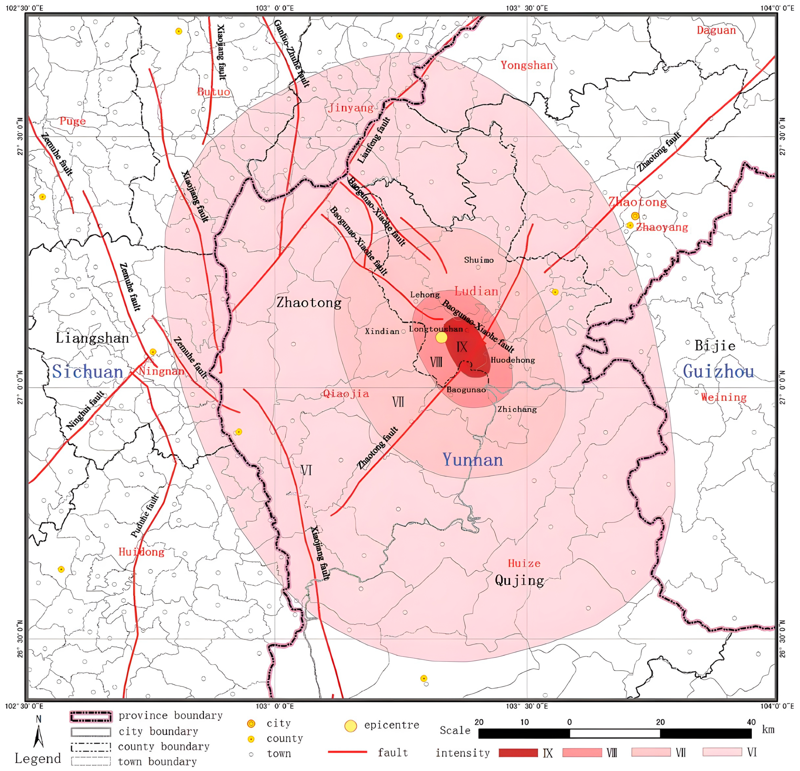
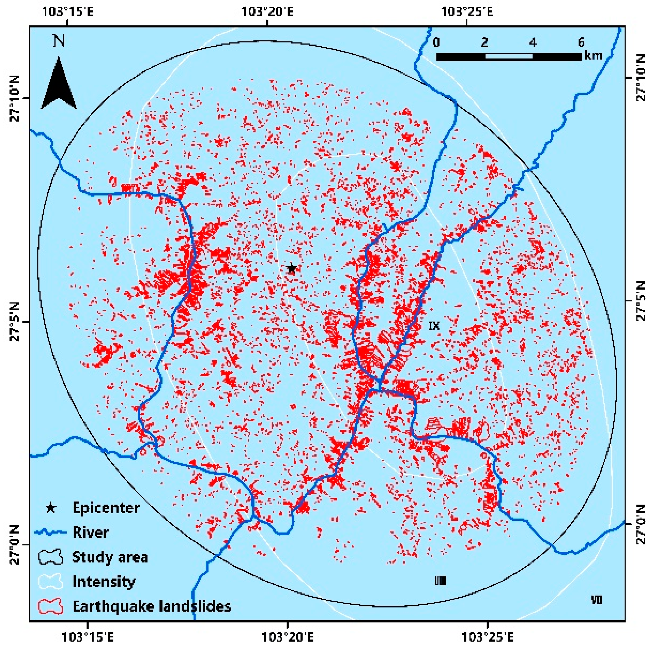
On 3 August 2014, a magnitude 6.5 earthquake struck Ludian County, Zhaotong City, Yunnan Province, China, with the epicenter located at 27.10°N, 103.34°E (Figure 1). This seismic event triggered a substantial number of coseismic landslides, exceeding 10,000 in total, with a combined area of 15 square kilometers [11]. The maximum intensity in the earthquake-affected area was nine on the seismic intensity scale (Figure 2). Seismic intensity refers to the degree to which the ground and various buildings in a certain area are affected by an earthquake. After an earthquake occurs, the seismic intensity in different areas away from the epicenter is evaluated based on the degree of building damage and changes in the ground surface, and equal intensity lines are drawn as a description of the degree of damage caused by the earthquake. Therefore, seismic intensity mainly indicates the degree of impact of earthquakes that have occurred [11]. The earthquake zone is situated in the lower reaches of the Jinsha River Basin, and the Niulan River traverses the earthquake area. This study utilizes the Ludian Earthquake Landslide Database, which includes 10,559 coseismic landslides induced by this earthquake (Figure 3) concentrated within the zones assigned intensity ratings of eight or nine [12]. Using the landslide interpretation area as the study area, this study introduces excess topography as a geomorphological indicator to explore its impact on the distribution of seismic landslides. Furthermore, to meet practical needs such as hydropower engineering planning, the input parameters were improved using a simplified Newmark model. The results include the regional landslide susceptibility distribution and earthquake landslide hazard zoning.

2. Regional Structural Background

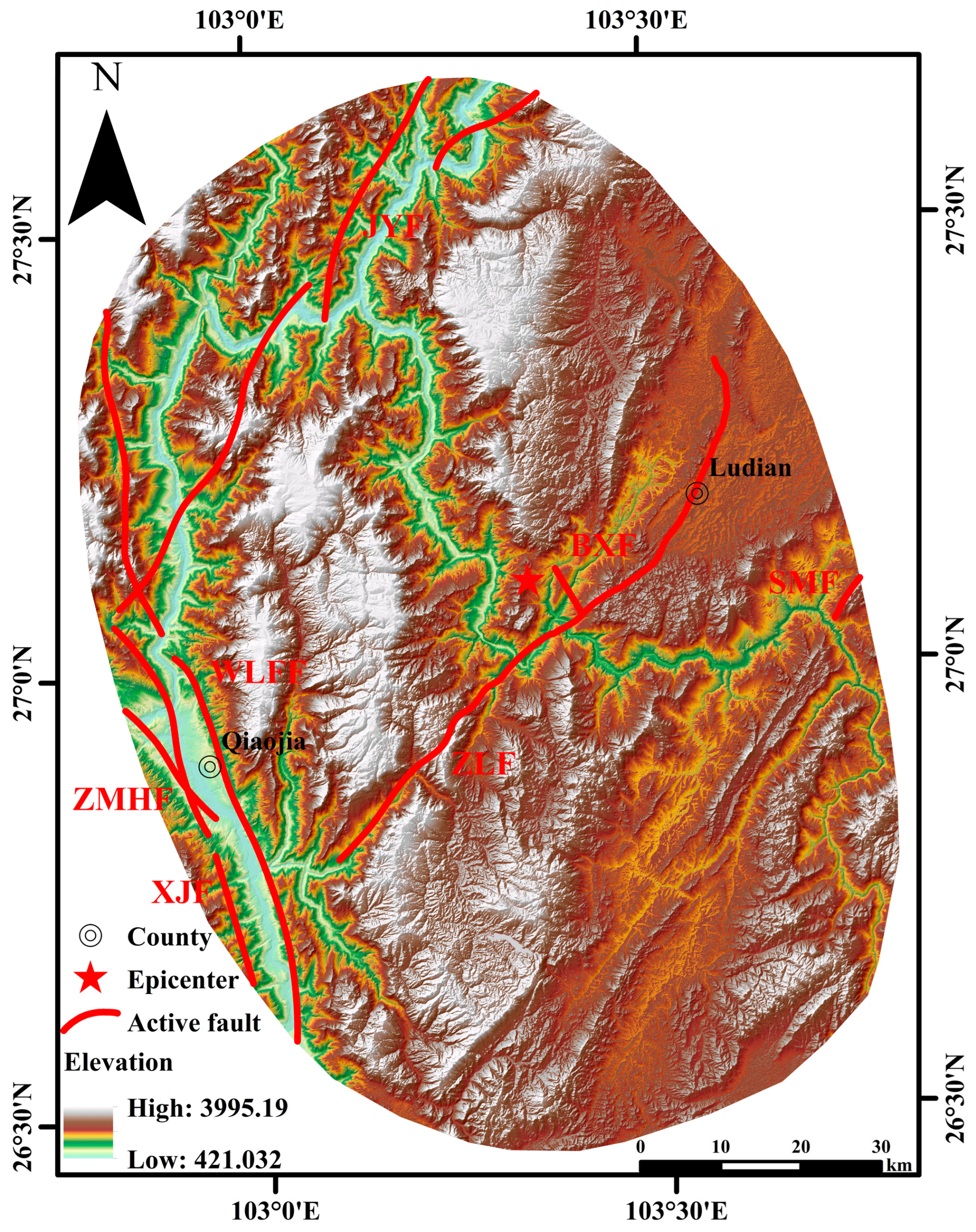
The Ludian Mw6.2 earthquake occurred at the eastern margin of the Qinghai-Tibet Plateau, east of the Sichuan Yunnan block, in the central southern section of the north-south seismic belt [13]. This earthquake was a moderate intensity earthquake that occurred on the deformation zone of the interaction boundary between the eastern edge of the Qinghai-Tibet Plateau and the South China Block, where the Sichuan Yunnan rhombic block moved in a southeast direction [14]. The Cenozoic tectonic deformation is strong here, with active faults of different orientations, and multiple earthquakes have occurred [15,16,17]. Figure 4 shows the distribution map of active structures in the region. The main controlling deep faults in the region are the north-northwest trending sinistral strike slip Zemuhe and Xiaojiang faults. There is also a series of small faults developing inside these fractured blocks. Northwest trending faults have also developed in this area, with the Zemuhe and Xiaojiang faults running from west to east.
The seismogenic fault of this earthquake is the Baogudang-Xiaohe Fault. The Baogudang-Xiaohe Fault is a secondary fault that matches the NE trending Lianfeng Fault, Zhaotong Ludian Fault Zone, and the SN trending Xiaojiang Fault. It has an average strike of N30 ° W and consists of several intermittently distributed faults. It starts from the Moon Mountain area north of Baogu Pass in the southeast, passes through Longtou Mountain, Lehong, Xiaohe, and Mantianxing in the northwest, and ends in the Dongping area. Along the fault, it is manifested as an outcrop section of fault pass and fault trough. The fracture zone is mainly composed of fault breccia, with clear scratches on the section. The lateral angle of about 30° indicates that the fault has left lateral strike slip and thrust properties [18].

3. Methods

3.1. Critical Slope

In regions with complex terrain, when the slope exceeds a certain critical value, it often triggers landslides and collapses. This critical value is referred to as the critical slope [19]. Carson and Petley have proposed the concept of the critical slope, believing that slopes are generally stable when the slope is less than the critical slope and require specific trigger factors to cause instability [19].
The uplift of the Earth’s surface has led to the deepening of features such as river systems and mountain ranges, making the slope steeper. However, due to factors such as cohesion and internal friction angle, the height and gradient of the slope cannot extend indefinitely and will eventually stabilize at a specific slope angle and on the slope surface, reaching what is known as the balanced state of the critical slope where the transformation of the landscape occurs to match the new conditions of the underlying layers, and a dynamic equilibrium is established [20,21,22,23].
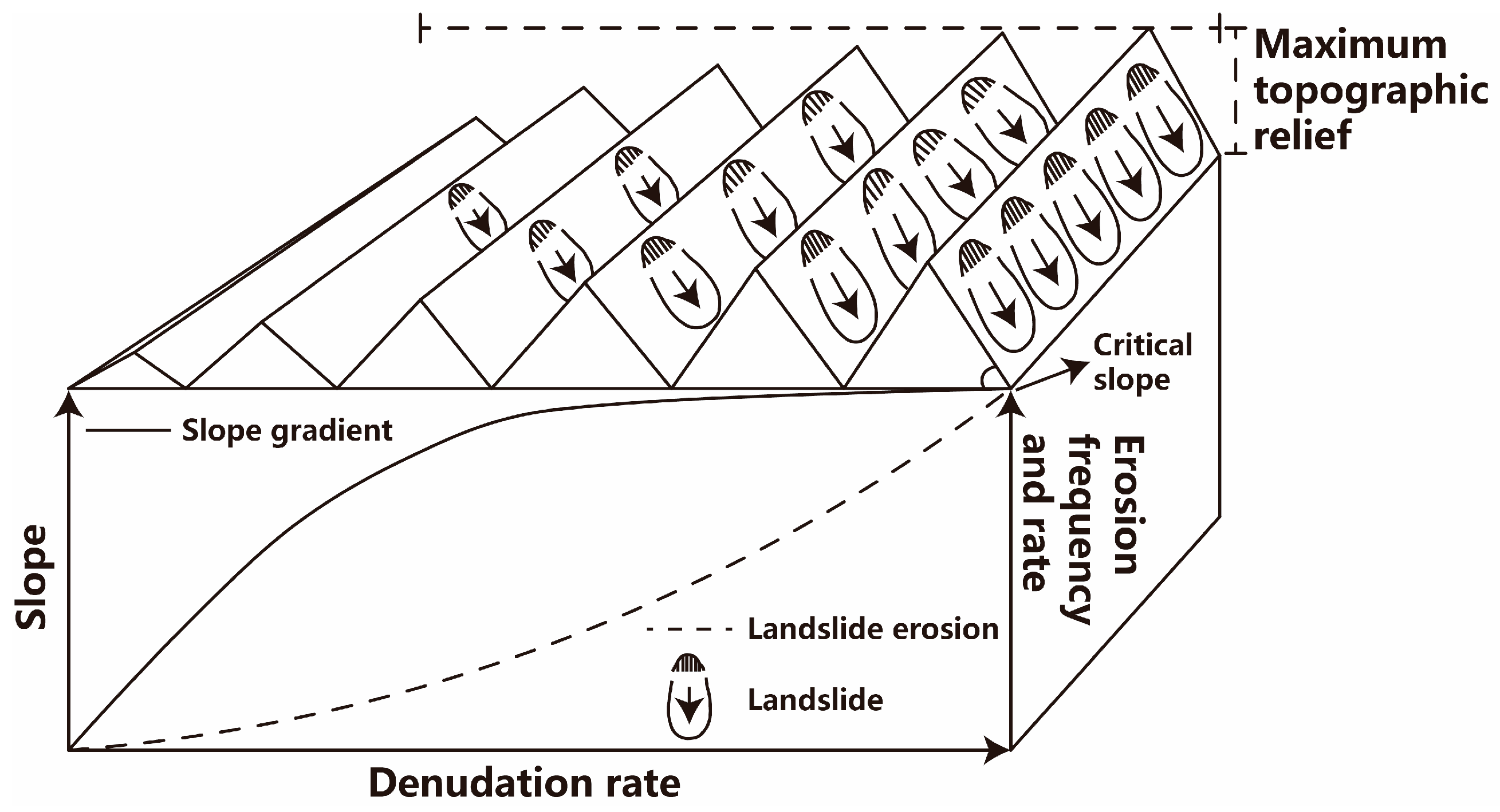
The growth of the slope gradient is not without limits (Figure 5). The frequency and speed of occurrence of events such as landslides will increase significantly with the gradient, but when it reaches the critical slope, the slope body will tend to stabilize, and the maximum geomorphic amplitude may be reached [24].
The excess topography beyond the critical slope is assumed to be a potentially unstable mountain body, and it is hypothesized that the critical slope exists continuously in the study area. Therefore, determining the exact value of the critical slope is essential for calculating excess topography, and terrain with a slope greater than the critical slope can serve as an indicator of the long-term impact of erosion on the slope body. Larsen and Montgomery’s study of landslides in the eastern Himalayas from 1974 to 2007 found that the frequency and rate of occurrence of slides are very low when the slope of the terrain is less than 30 degrees, but they increase significantly when the slope approaches or exceeds 30 degrees, with shallow, frequently occurring slides becoming the main form of erosion despite differences in river water power of several orders of magnitude [25]. Numerous studies have shown that the critical slope typically ranges from 30 to 35 degrees in deep, narrow canyons where the difference in elevation is significant and the slope is steep [21,26,27,28,29,30]. When researching the overloaded terrain of the Qilian Mountains and the southeastern edge of the Tibetan Plateau, Blöthe and Liu both use 30 degrees as the value of the critical slope [29,31].
The internal friction angle is a measure of the ability of soil or rock particles to resist shear movement due to friction, and it is also an indication of how much positive stress a rock mass can bear before it starts sliding along the critical plane. A larger internal friction angle means higher stability and bearing capacity of the rock mass [21]. The critical slope is the hypothetical value at which the rock mass begins to lose its stability and slide along the critical plane. Therefore, instead of using different values for the critical slope as previous researchers have done, we propose treating the critical slope as the internal friction angle, which controls the stability of the rock mass.

3.2. Excess Topography

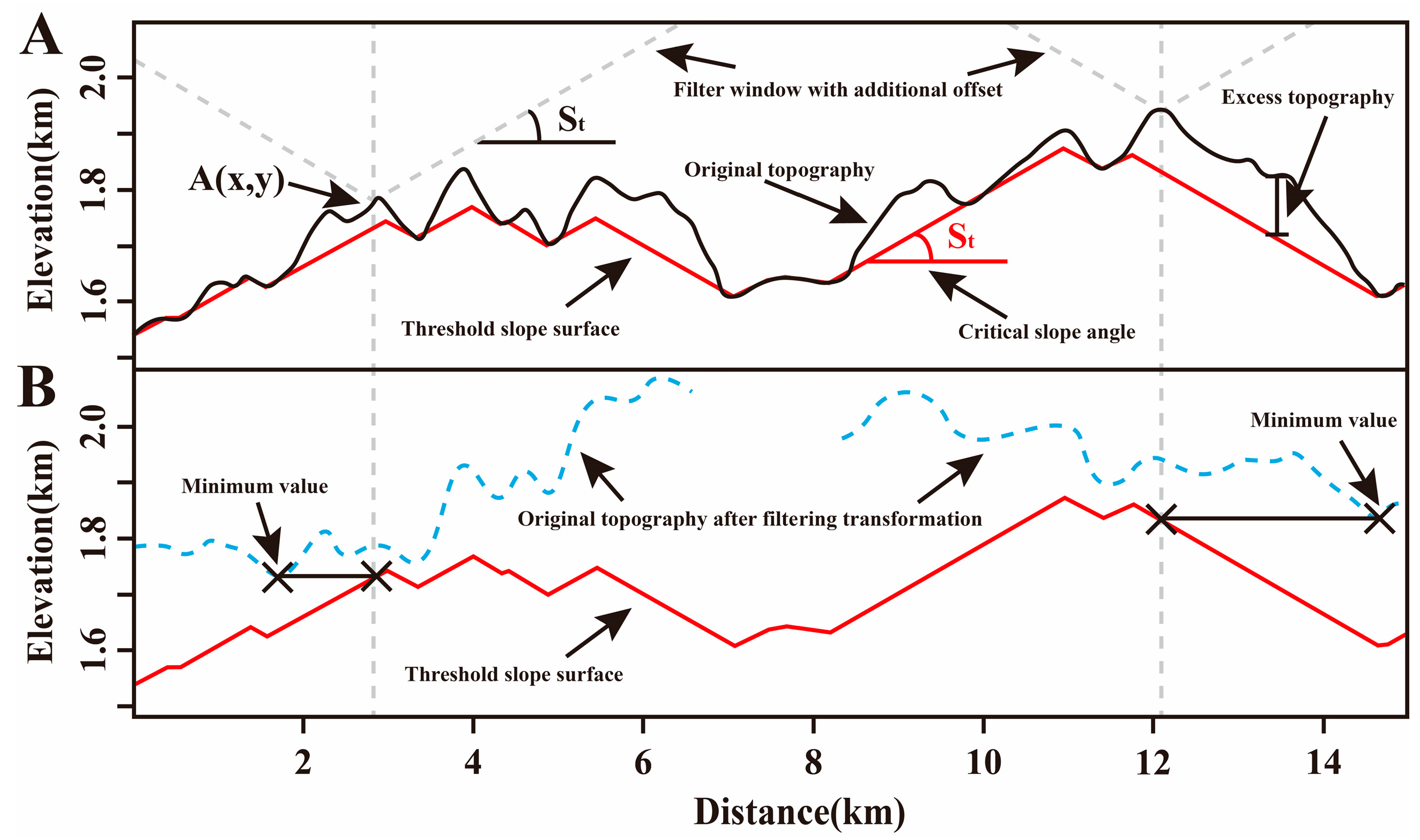
Blöthe introduced the concept of excess topography based on the critical slope to represent potentially unstable masses within a mountain where the slope exceeds the critical slope (Figure 6) [29]. Therefore, excess topography can be considered as the potential source material for landslides. Quantifying excess topography is crucial for understanding the importance of slope erosion in regional landform evolution and provides a clear indication of the risk of new landslides.
By using a digital elevation model (DEM) with projection information as input data, the calculation formula for the critical slope at a specific point A (x, y) is
Z ˙ x , y = min s , t , Z x + s , y + t + s t s 2 + t 2
where Z represents the actual terrain elevation, Z ˙ represents the idealized critical slope surface elevation, s t is the tangent value of the critical slope, and s and t are the filter coefficients, indicating the distance from the filter center to the point (x, y).
By setting the filter angle based on the given critical slope angle, the actual terrain is processed through the filtering calculation formula to obtain the filtered terrain. When the minimum value of the filtered terrain deviates from the center of the filter, the critical slope surface is lower than the actual terrain, indicating the presence of excess topography.
The elevation of the excess topography Z can be obtained by subtracting the elevation of the critical slope surface Z E from the actual terrain elevation,
Z E x , y = Z x , y Z ˙ x , y
The extraction of the excess topography is performed on the 12.5 m DEM of the study area through Matlab’s TopoToolbox [32].

3.3. Newmark Model

The Newmark cumulative displacement model, proposed based on the limit equilibrium theory, is a widely used method for assessing slope stability under seismic conditions [33]. Jibson simplified the model to make it more suitable for regional assessments. In this model, the critical acceleration is used to measure the potential risk of earthquake-induced landslides in a region [5]. The higher the critical acceleration, the greater the external force the slope can resist, indicating stronger stability. Conversely, a lower critical acceleration suggests that the slope is less stable.
In a static state, the static safety factor can be calculated using the infinite slope method
F S = m g cos α tan φ m g sin α = tan φ tan α
where m represents the mass of the sliding block, F S is the static safety factor, g is the acceleration due to gravity, and α is the inclination angle of the sliding surface, which can be approximated by the slope angle of the slope body. The term m g cos   α tan   ϕ represents the resisting force, while m g sin α represents the driving force.
m g sin α + m a c m g cos α tan φ = 1
Transforming the equation allows the calculation of the critical acceleration a c of the sliding block,
a c = tan φ tan α 1 g sin α
approach,
a c = F S 1 g sin α
Considering the influence of the effective internal friction angle and cohesion of the geotechnical material on the static slope stability, F S can be calculated as follows,
F S = c γ t sin α + tan φ tan α m γ w tan φ γ tan α
where c is the effective cohesion of the slope geotechnical material, φ is the effective internal friction angle, t is the thickness of the sliding mass, m is the ratio of the saturated portion to the total thickness of the sliding mass, γ is the unit weight of the geotechnical material, and γ m is the unit weight of water.
Based on the results of a regional landslide susceptibility survey, this study selected the widely used peak ground acceleration measurement as the main input parameter for a regional earthquake landslide hazard assessment [5,34,35,36]. By comparing a c with PGA, the potential hazard of seismic landslides in the area can be quickly assessed. The greater the difference between PGA and the critical acceleration a c , the higher the hazard of seismic landslides.

4. Extraction of Excess Topography in the Ludian Earthquake Study Area

4.1. The Value of the Critical Slope

The internal friction angle indicates the ability of soil or rock particles to resist shear movement due to friction. Similarly, the internal friction angle is a measure of how much normal stress a geotechnical material can withstand without slipping when subjected to shear stress. Therefore, compared to previous studies that uniformly assigned critical slope values to the study area, this paper suggests considering the critical slope as the internal friction angle that controls the stability of geotechnical slopes.
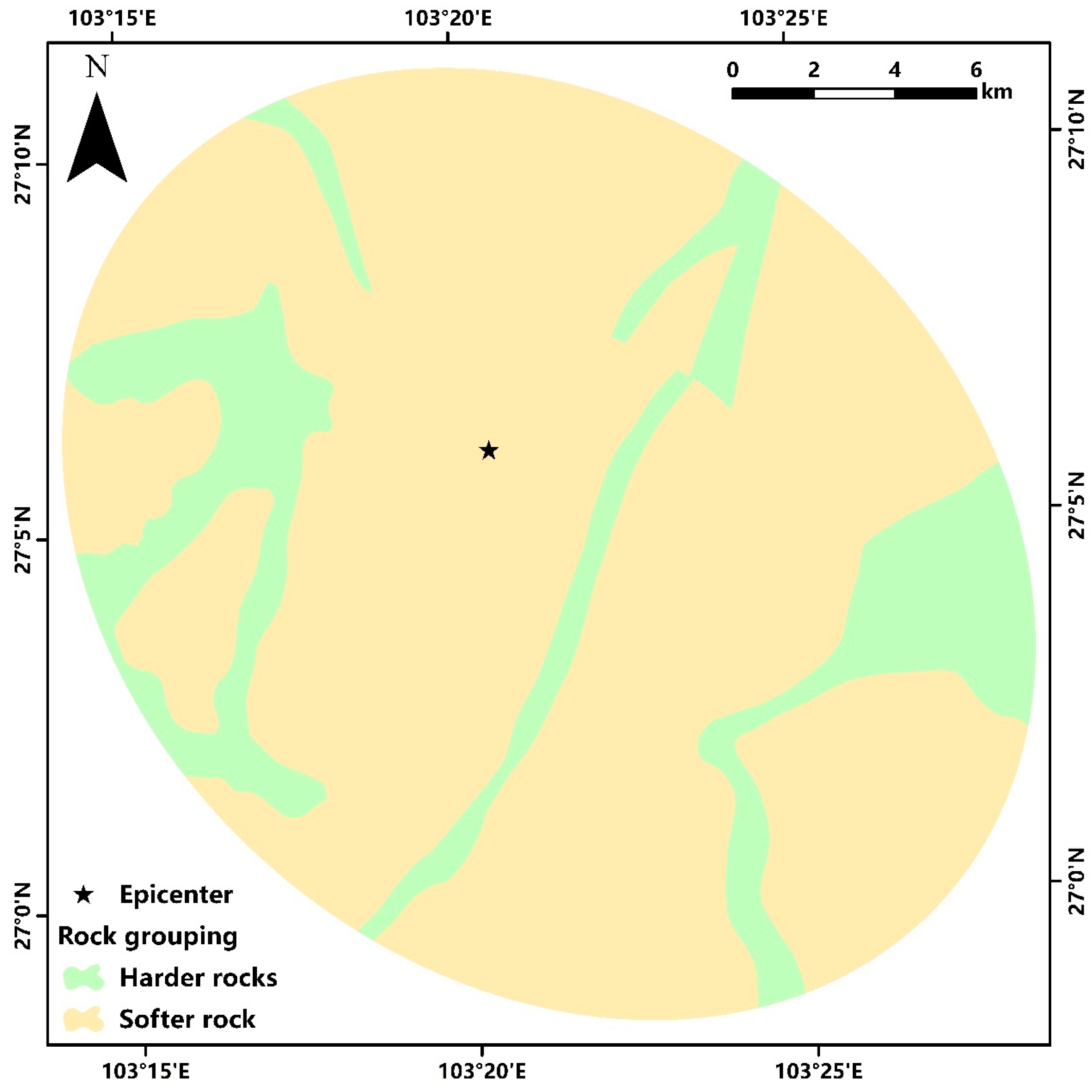
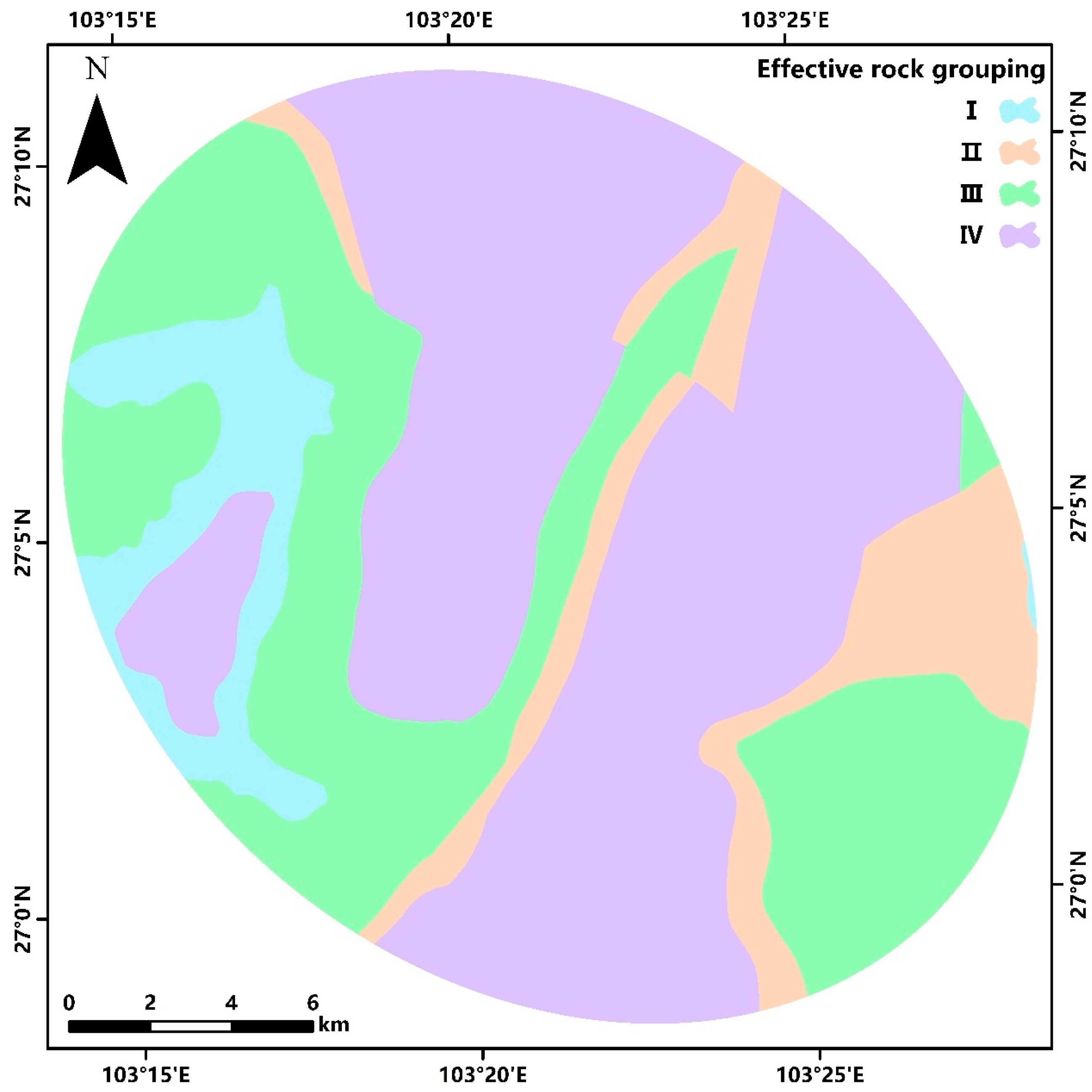
The lithology in the Ludian earthquake study area primarily includes basalt, limestone (including dolomitic limestone), dolomite (including algal dolomite), shale, sandstone, siltstone, mudstone, and coal seams. Based on rock properties, the strata in the study area are classified into two categories: harder rock and softer rock (Figure 7). According to previous research, the average internal friction angle of different rock groups is used as the critical slope for the corresponding rock types (Table 1).
The determination of the critical slope is influenced by various factors, such as soil properties, geological structure, rainfall intensity, and groundwater. Different regions and types of soils may have different critical slopes. Studies have shown that as rainfall gradually infiltrates, the physical properties of the soil change, which may lead to a reduction in soil strength and affect the critical slope. For instance, some research has found that prolonged rainfall can cause the dissolution and migration of bonding materials in the soil, resulting in changes in the soil’s porous structure and a subsequent decrease in its resistance to shearing forces, leading to a smaller critical slope. Additionally, geological structures and topographic features also play a role in affecting the critical slope. For example, in regions with complex geological structures, the presence of faults and folds can reduce the stability of the slope and make the critical slope smaller. Human activities, such as irrigation projects and slope excavations, can also alter the distribution of groundwater and the physical properties of the soil, thereby affecting the critical slope [37,38,39,40]. Therefore, future research needs to explore the relationship between the internal friction angle and the critical slope in detail to determine the precise internal friction angle.

4.2. Extraction of Excess Topography

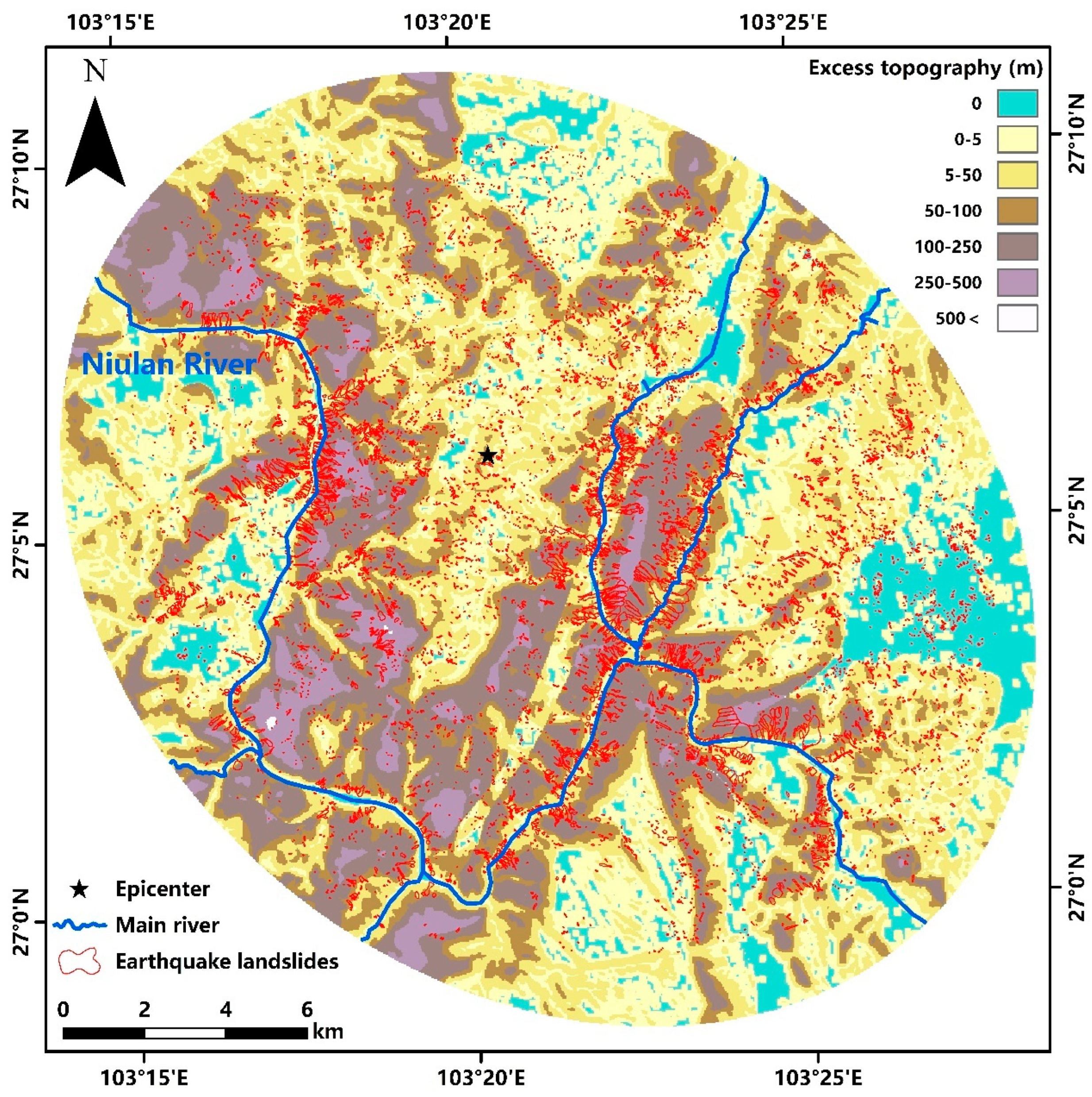
Based on the critical slope values and DEM, the excess topography of the Ludian earthquake area was extracted. The extraction results were reclassified into seven groups of excess topography intervals (Figure 8). Among them, 0 represents non-excess topography areas, while the remaining groups contain the maximum values within each interval. The maximum value of the excess topography is 548.28 m. It can be seen that extremely high excess topography is distributed in the high and steep valleys on both sides of the Niulan River and extends along the river, while lower excess topography is distributed in relatively flat areas. The amount of excess topography is relatively large near the ridgeline. In the study area, non-excess topography areas account for about 8.53%, with the majority of excess topography in the 5–50 m interval, covering approximately 29.82% of the area.

4.3. Validation of the Correlation Between Seismic Landslides and Excess Topography

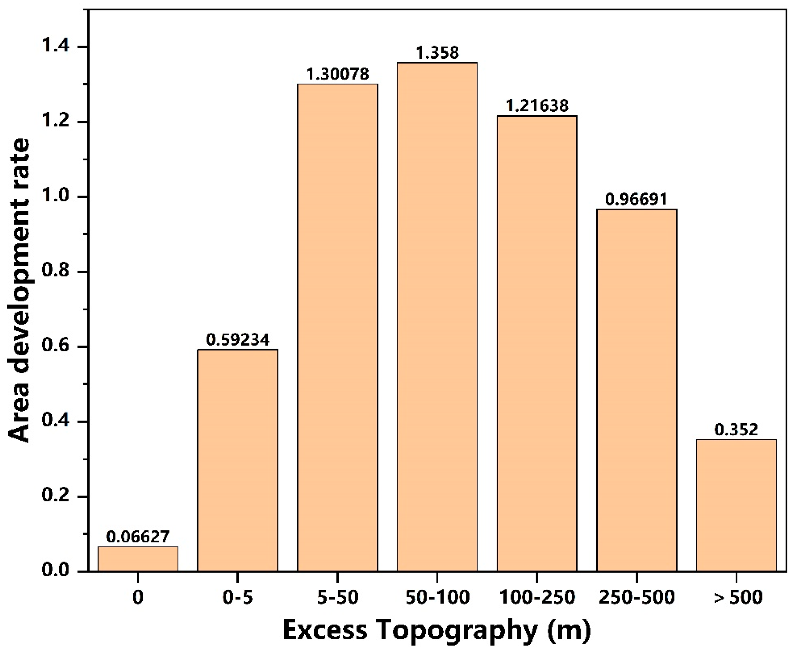
To visually compare the frequency of seismic landslides occurring in different excess topography intervals, the concept of landslide development rate is introduced for analysis [2]. A development rate of 1 indicates that the contribution of that excess topography interval to the seismic landslide area in the study area is proportional to its exposure area in the study area, representing the average probability of seismic landslide development for excess topography in the study area. If the development rate is less than 1, it indicates that the probability of seismic landslides occurring within that excess topography interval is below the average level of the study area, signifying a less prone landslide area. Conversely, if the development rate is greater than 1, it indicates that the excess topography interval is a landslide-prone area within the study area.
Through comparative analysis (Figure 9), it was found that the development rate of seismic landslides is highest in the excess topography interval of 50–100 m, at approximately 1.36. This is followed by the intervals of 5–50 m and 100–250 m, with seismic landslide development rates of about 1.30 and 1.22, respectively, indicating that the interval of 50–250 m is a landslide-prone area in the study region. In the interval of 250–500 m, the seismic landslide development rate is about 0.97, which is close to 1, indicating that this interval represents the average level of seismic landslide development in the study area. In the non-excess topography area, the development rate of seismic landslide area is less than 0.07, nearly 0, indicating a very low development rate of seismic landslides in areas without excess topography, which is consistent with natural principles. In the interval of 0–5 m of excess topography, the development rate of seismic landslides is about 0.59, indicating that this interval is a less landslide-prone area in the study region, suggesting that when the amount of excess topography is low, seismic landslides are less likely to be triggered. In areas where the excess topography exceeds 500 m, the development rate of seismic landslide areas is only 0.35, making it another less landslide-prone area in the study region. One reason for this is that the area of excess topography greater than 500 m constitutes only 0.017% of the total study area, which is relatively small, resulting in fewer triggered landslides. Additionally, excess topography represents the potential landslide body thickness above the ideal stable slope surface, and a thickness greater than 500 m is relatively large. The seismic intensity required to trigger landslides in such areas should also be higher. It is possible that the intensity of the earthquake in these regions was not sufficient to meet the conditions for triggering landslides, resulting in a lower development rate for this interval.

5. Landslide Susceptibility Distribution in the Ludian Earthquake Study Area

5.1. Parameter Values for the Newmark Model

Due to the lack of sufficient measured rock strength parameters and clear reduction relationships, this study appropriately reduced the empirical values of each rock group in the examples in the table based on the physical and mechanical properties of the rock and soil in the study area, using them as effective strength parameters. The hardness and mechanical properties of engineering geological rock formations, as well as the distribution of rock formations, the stability, sturdiness, cracks and permeability of mountains, and the weathering resistance of formations all significantly affect the geological conditions of the study area. The reduction coefficients are shown in Table 2. Multiplying the reference values of internal friction angle and cohesion with the loss coefficient can obtain the effective internal friction angle and effective cohesion (Table 3), as well as the grouping distribution of rock mechanics parameters (Figure 10).
Based on regional hydrogeological surveys, it is known that the Ludian earthquake study area primarily consists of lava, pores, and fractures in igneous and metamorphic rocks. Wells in these formations yield less than 50 cubic meters per day, and the flow rates of underground rivers and springs are less than 1 L per second. These rock layers have very low water content, with a defined saturation of 0. Secondly, the area includes karst, fractures, and caves in carbonate rocks. Wells in these formations yield between 350 and 1750 cubic meters per day, and the flow rates of underground rivers and springs range from 0.7 to 3.5 L per second. These rock layers have higher water content, with a defined saturation of 0.25.
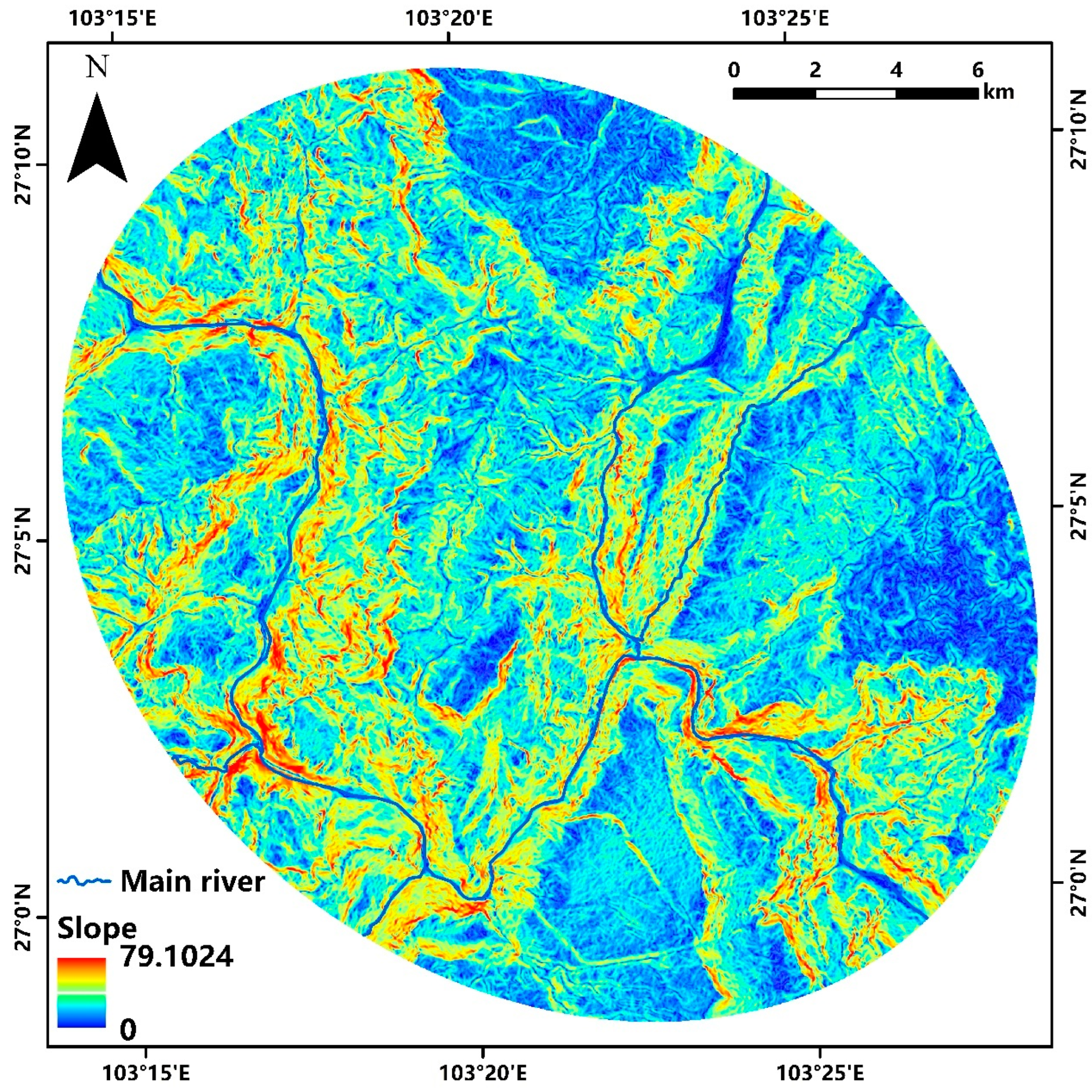
Due to the predominance of shallow landslides induced by earthquakes [37], and based on previous studies, the landslide thickness in the Ludian earthquake study area is uniformly assigned a value of 3 m [18,41,42,43]. The slope distribution in the study area was calculated using ALOS 12.5 m DEM data (Figure 11), showing that the maximum slope in the Ludian earthquake study area reaches 79°. High and steep areas are commonly found in the valleys on both sides of the rivers.

5.2. Landslide Susceptibility Assessment

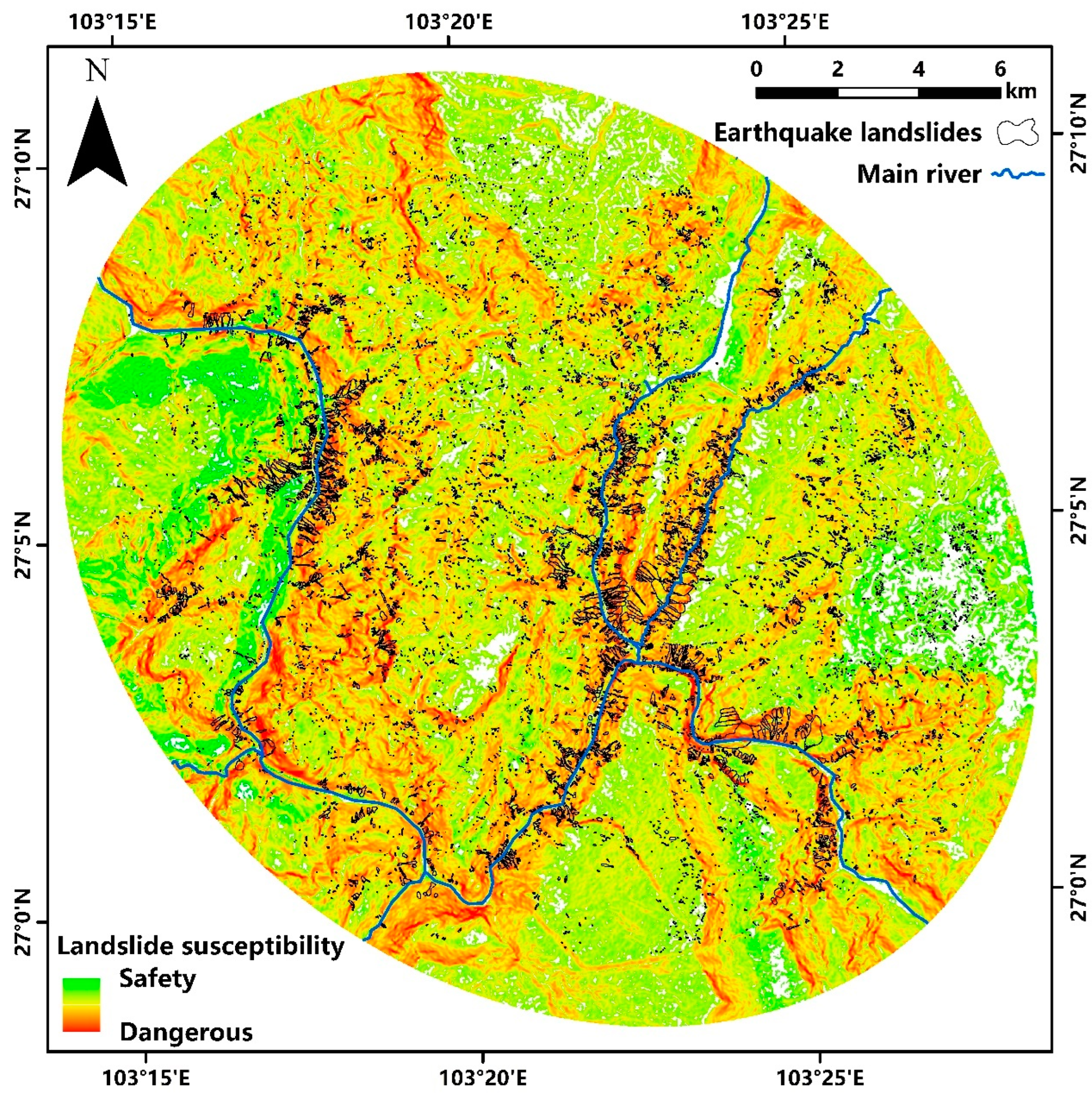
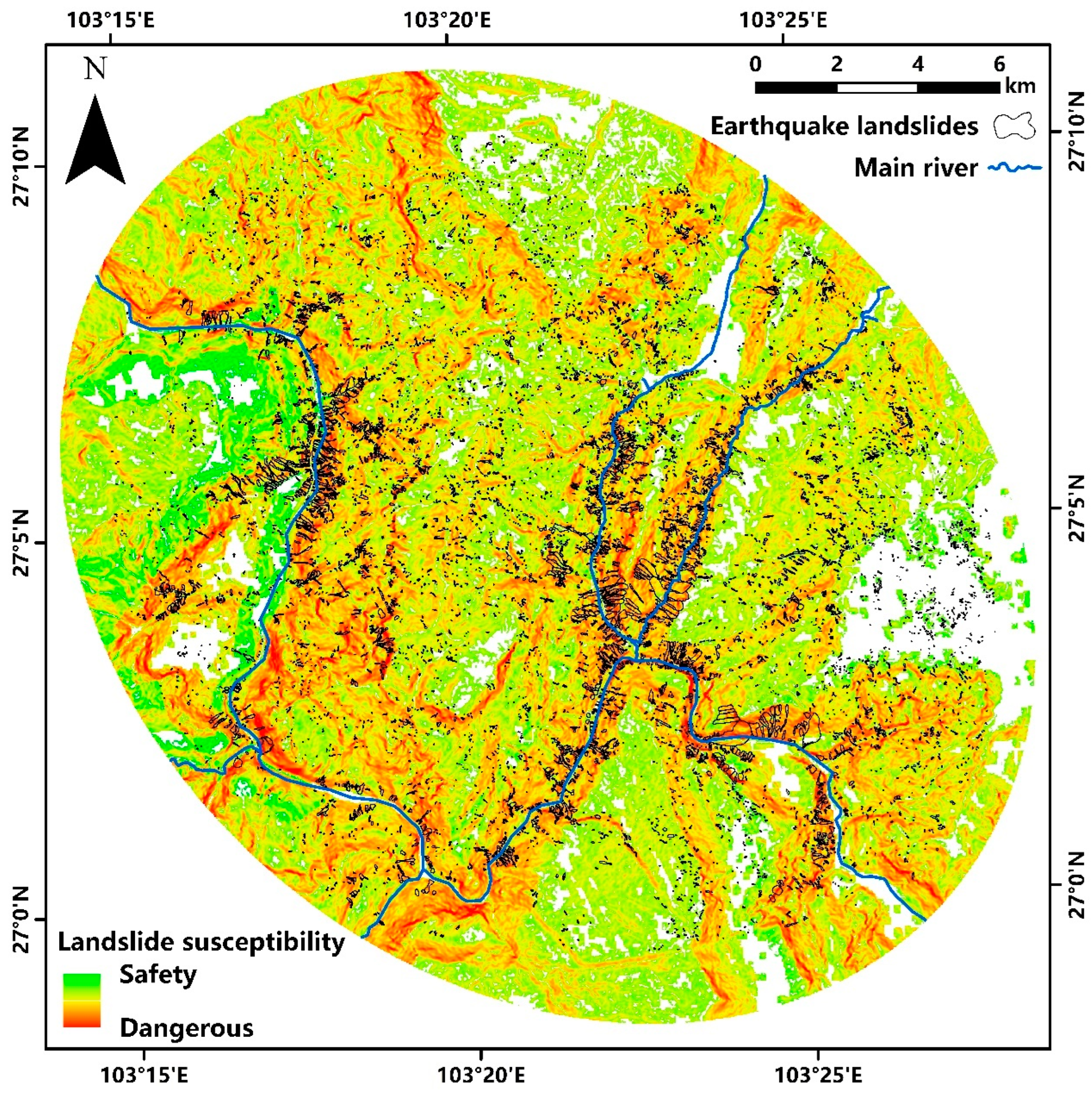
Using the obtained effective internal friction angle, effective cohesion, unit weight of geotechnical material, thickness of the sliding mass, saturation of geotechnical material, water density (uniform value of 1 g/cm3), and slope, the landslide susceptibility distribution in the Ludian earthquake study area was calculated (Figure 12). In the landslide susceptibility distribution map, the transition from red to green indicates a gradual decrease in landslide susceptibility. Areas with higher susceptibility suggest that these regions are more prone to slope movement under external forces, constituting potential risk zones. It can be observed that the steep slopes on both sides of the rivers exhibit higher risk, with coseismic landslides predominantly developing in areas with higher landslide susceptibility. Since this susceptibility assessment does not account for regional differences in seismic ground motion levels, it cannot display the probability of landslide occurrence under various seismic conditions in different areas. Therefore, it is necessary to further evaluate the seismic landslide hazard in the study area.

5.3. Model Accuracy Validation

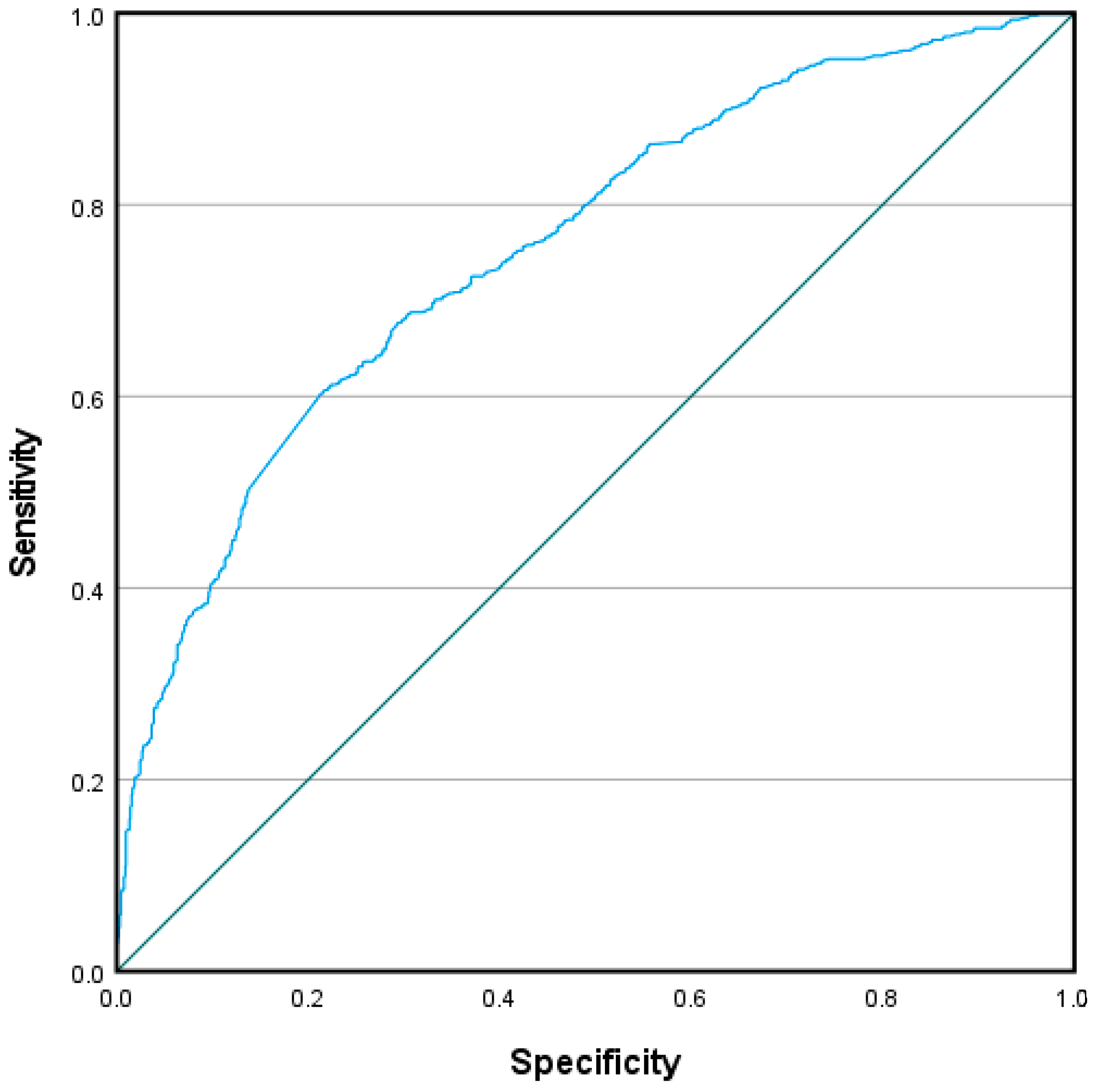
The ROC curve is a tool used to evaluate and compare the performance of binary classification models [44,45]. It demonstrates the model’s classification ability by plotting the true positive rate against the false positive rate at various threshold levels. This method can be used to assess the accuracy of geological hazard susceptibility evaluations. The area under the ROC curve (AUC) is an indicator of the performance of the classification model, with values ranging from 0 to 1. The closer the AUC value is to 1, the stronger the model’s predictive capability, indicating superior model performance.
Using the 10,559 landslide centers within the Ludian earthquake study area as landslide sample points, and randomly selecting 10,000 non-landslide points outside the landslide areas as non-landslide sample points, a total of 20,559 sample points within the Ludian earthquake study area were analyzed. By extracting the critical acceleration value corresponding to each sample point, an ROC curve analysis was conducted (Figure 13). The AUC value of this curve is 0.755, indicating that the landslide susceptibility evaluation results are effective and the model’s actual predictive accuracy is relatively high. Given the small size of the study area and the high density of sample points selected within the study area, the AUC value might be slightly lower due to potential sample selection bias. Since the landslide susceptibility analysis results were obtained prior to the occurrence of the Ludian earthquake, it suggests that these results are applicable to real-world scenarios.

5.4. Validation of the Correlation Between Landslide Susceptibility and Excess Topography

Two-variable correlation analysis is a statistical method used to assess whether there is a linear relationship between two variables and the degree of that relationship [46]. After conducting normality tests on the excess topography and critical acceleration in the Ludian earthquake study area, it was found that these two variables do not follow a normal distribution. The degree of correlation is typically measured using a correlation coefficient. The Spearman’s rank correlation coefficient is used to measure the correlation between the ranks (or order) of two variables [47,48]. It is suitable for ordinal data or continuous data that do not completely follow a normal distribution.
In the Ludian earthquake study area, 10,000 sample points were randomly selected, and the excess topography values and critical acceleration values were extracted for each. A Spearman’s correlation analysis was conducted on these two sets of variables (Table 4), resulting in a correlation coefficient of −0.771. According to the critical values table for the Spearman’s rank correlation coefficient test, this result rejects the null hypothesis, indicating a significant correlation. The two-tailed test results show a very significant negative relationship between the two variables. The larger the critical acceleration value, the more stable the landslide susceptibility. The Spearman correlation coefficient indicates that as the critical acceleration increases, the excess topography decreases. This can be understood as the smaller the excess topography, the more stable the landslide susceptibility. This also demonstrates that excess topography can be used as a reference indicator for the potential occurrence of landslides and as a parameter for predicting landslide susceptibility.

5.5. Landslide Susceptibility Analysis Incorporating Excess Topography

Given the significant correlation between excess topography and landslide susceptibility, it indicates that excess topography can serve as a reference indicator for potential landslide thickness. Therefore, the average excess topography for different intervals in the Ludian earthquake area was calculated. Considering the possible thickness of actual landslides, the average excess topography for different intervals was adjusted using a proportional coefficient to represent the potential landslide thickness (Table 5). It is assumed that non-excess topography areas do not have potential landslide bodies.
Combining the potential landslide thickness with adjustments based on the excess topography, a new landslide susceptibility distribution for the Ludian earthquake study area was calculated (Figure 14). It can be seen that this result differs from the uniform 3-m assignment. High landslide risk areas are still located in the steep slopes on both sides of the rivers. Coseismic landslides are more prevalent in areas with higher landslide susceptibility. However, there are still some small landslides in non-dangerous areas, which may be debris flows triggered by loose rock fragments on the slope surface due to seismic vibrations.
Using the 20,559 sample points within the Ludian earthquake study area, an ROC curve analysis was performed on the new landslide susceptibility results (Figure 15). The AUC value of this curve is 0.829. This indicates that the landslide susceptibility evaluation result is better and has higher accuracy compared to the uniform 3-m thickness assignment. Judging by the AUC value, this result is relatively consistent with reality and can be applied to seismic landslide hazard prediction analysis.

6. Earthquake Landslide Hazard Prediction in the Ludian Earthquake Area

Under the influence of an earthquake, the stability of a slope is determined by both the properties of the slope itself and the magnitude of the seismic forces it experiences. Therefore, by comparing the critical acceleration of the slope with the peak ground acceleration (PGA) of the seismic motion, the earthquake landslide hazard areas in the study region can be assessed. This method allows for the identification of regions where the potential for landslides is high, providing valuable information for hazard mitigation and planning.

6.1. Actual Ground Motion Conditions

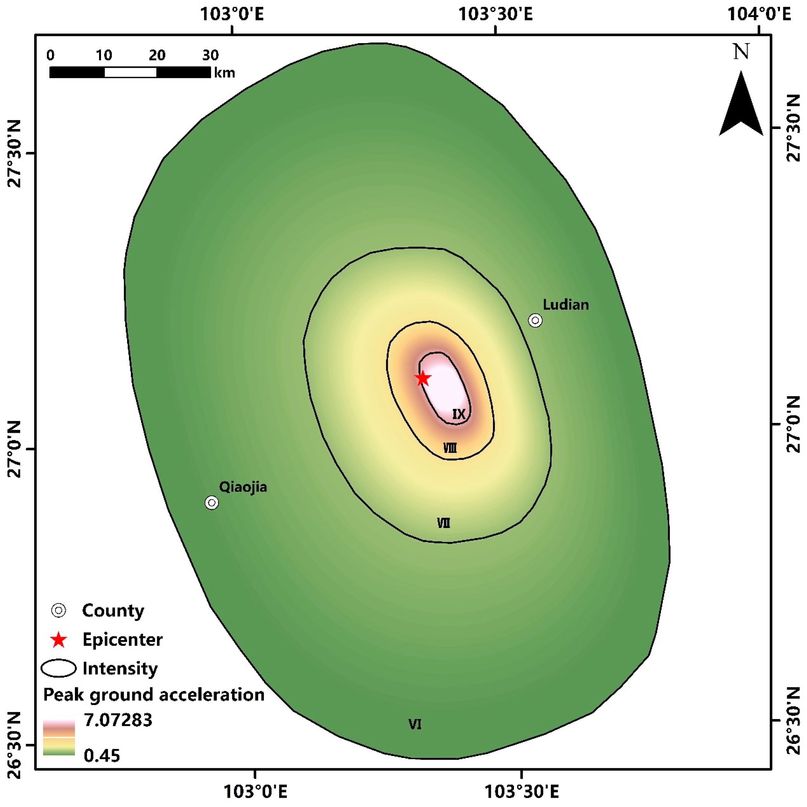
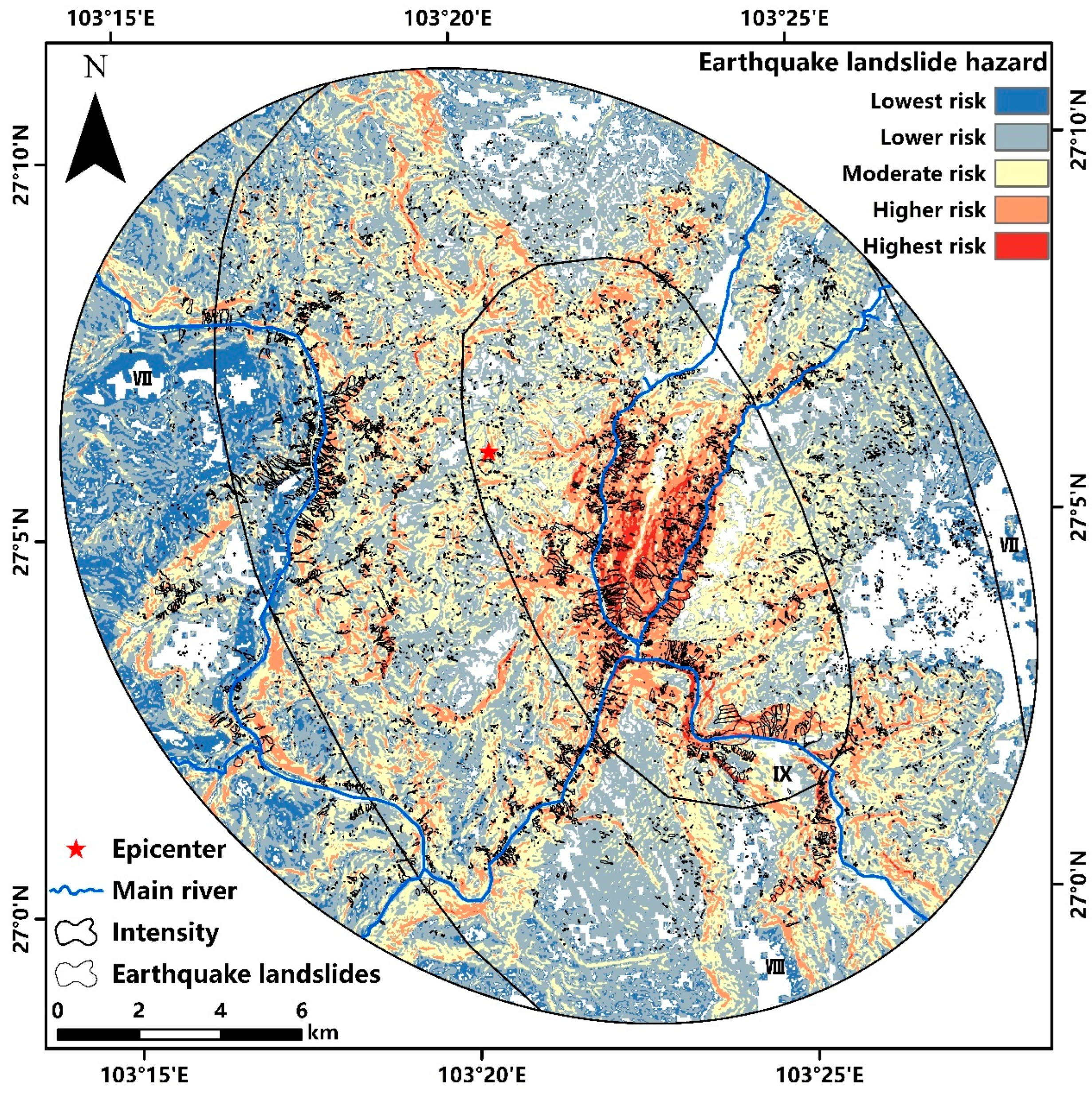
Based on the conversion method between seismic intensity and peak ground acceleration (PGA) for the Ludian earthquake (Table 6) [42], the PGA distribution map for this event was obtained (Figure 16). Using this information and the landslide susceptibility calculations, the earthquake landslide hazard distribution map for the Ludian earthquake study area was created (Figure 17), categorizing the hazard into five levels: extremely high risk, high risk, moderate risk, low risk, and extremely low risk. The area proportions for each hazard zone are 10.33%, 43.06%, 31.77%, 13.57%, and 1.28%, respectively. The results show that on both sides of the rivers in the southeast of the epicenter, within the IX intensity zone, the earthquake landslide hazard is generally extremely high. Relatively large landslides are densely distributed in this area. The relatively higher risk zones are almost aligned along the riverbanks. Similarly, in the upstream area of the Niulan River to the west of the epicenter, the hazard is also relatively high with a dense distribution of landslides.
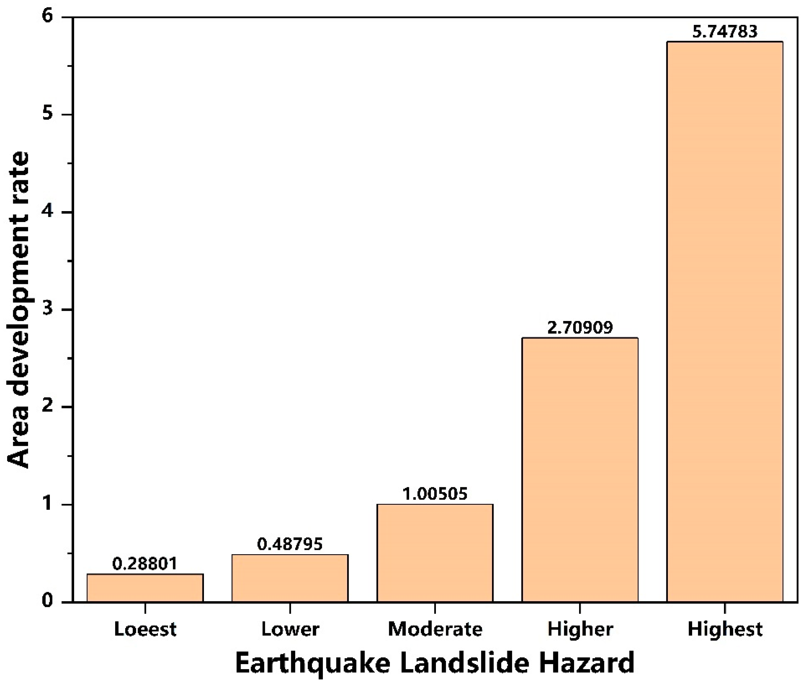
By calculating the seismic landslide area development rates for different hazard zones (Figure 18), it was found that the development rate in the moderate hazard zone is approximately 1. This indicates that the moderate hazard zone represents the average level of landslide development under the current seismic conditions in the study area. In the extremely low hazard zone, the development rate is only 0.29, while in the low hazard zone, it is 0.49. These two areas are less prone to landslides in the study area for this earthquake. In contrast, the development rate in the high hazard zone is 2.71, and in the extremely high hazard zone, it reaches 5.75. This shows that these two zones are highly prone to landslides in the study area for this earthquake, with the extremely high hazard zone being particularly susceptible to landslides. This seismic hazard prediction result can provide valuable reference and suggestions for emergency response and post-disaster reconstruction efforts.

6.2. Basic Ground Motion Conditions

According to the Chinese Seismic Ground Motion Parameter Zonation Map, the Ludian earthquake study area falls within the 0.15 g PGA range. Using the basic PGA and critical acceleration, an analysis was conducted to predict earthquake landslide hazards based on a 10% exceedance probability in 50 years (Figure 19). This figure represents a conventional pre-earthquake seismic landslide hazard prediction for the region. The area proportions for the extremely low hazard zone, low hazard zone, moderate hazard zone, high hazard zone, and extremely high hazard zone are 21.97%, 38.93%, 27.96%, 9.30%, and 1.84%, respectively. Since the basic ground motion is more uniformly distributed compared to actual seismic motion within the study area, the resulting hazard distribution is also more evenly spread. The results indicate that the extremely high and high seismic landslide hazard zones in the Ludian earthquake study area are almost exclusively distributed along the rivers.
By calculating the seismic landslide area development rates for different hazard zones (Figure 20), it was found that the development rate in the moderate hazard zone is approximately 1.36, close to 1. This indicates that the moderate hazard zone still represents the average level of landslide development within the study area. In the extremely low hazard zone and low hazard zone, the seismic landslide development rates are about 0.43 and 0.66, respectively. These two zones remain less prone to landslides under basic ground motion conditions, but the development rates are higher compared to the actual seismic motion results. In the high hazard zone and extremely high hazard zone, the seismic landslide development rates are approximately 2.30 and 2.93, respectively. This indicates that these two zones are also landslide-prone areas within the study region, but the development rates are lower compared to the actual seismic motion results. Although the seismic landslide hazard zoning results based on the basic peak ground acceleration differ somewhat from those based on actual seismic motion, they still align with objective principles. This indicates that the seismic hazard prediction results are realistic and can provide valuable references and suggestions for pre-earthquake urban planning, engineering construction, and other disaster prevention and mitigation efforts.

7. Conclusions

This study focuses on the VIII and IX intensity zones of the Ludian earthquake area. Excess topography in the study area was extracted and analyzed for its correlation with seismic landslides. The landslide susceptibility and earthquake landslide hazard in the study area were calculated. The results are as follows:
(1)
The maximum value of excess topography in the study area is 548.28 m. Extremely high excess topography is distributed in the high and steep valleys on both sides of the Niulan River and extends along the river. The amount of excess topography is relatively large near the ridgeline. The non-excess topography area accounts for about 8.53% of the study area. The interval with the most excess topography is 5–50 m, covering approximately 29.82% of the area. The intervals of 50–500 m are prone to landslides in the study area, while intervals below 50 m and above 500 m are less prone to landslides.
(2)
A landslide susceptibility analysis was conducted for the study area, assuming a uniform potential landslide thickness of 3 m. The Spearman’s rank correlation coefficient between the critical acceleration values and excess topography was calculated, yielding a correlation coefficient of −0.771. This indicates a strong and significant negative correlation between excess topography and critical acceleration.
(3)
By setting the potential landslide thickness based on excess topography and proportional coefficients, a new landslide susceptibility distribution was obtained. ROC curve analysis showed that the AUC value of the new results is 0.829, higher than the original AUC value of 0.755, indicating higher model evaluation accuracy with the new approach.
(4)
Earthquake landslide hazard predictions were made for both post-earthquake rapid assessment using actual ground motion and pre-earthquake planning using a 2% exceedance probability in 50 years. The results were verified against landslide development rates and were found to be consistent with actual conditions.

Author Contributions

Conceptualization, P.Z.; methodology, P.Z., X.C. and Q.Z.; validation, P.Z., H.X. and Z.L.; formal analysis, P.Z. and X.C.; investigation, P.Z.; resources, P.Z. and C.X.; data curation, P.Z. and C.X.; writing—original draft preparation, P.Z.; writing—review and editing, P.Z., X.C., Q.Z., H.X. and Z.L.; visualization, P.Z.; supervision, P.Z., X.C. and Q.Z.; project administration, X.C.; funding acquistion, X.C. All authors have read and agreed to the published version of the manuscript.

Funding

This research was funded by the National Nonprofit Fundamental Research Grant of China, Institute of Geology, China Earthquake Administration (Grant No. IGCEA2202).

Data Availability Statement

Data associated with this research are available and can be obtained by contacting the corresponding author.

Acknowledgments

We appreciate the editors and reviewers for their valuable comments that greatly improved the paper.

Conflicts of Interest

Authors Pengfei Zhang, Haibo Xiao and Zhiyuan Li are employed by the company Power China Beijing Engineering Corporation Limited. The remaining authors declare that the research was conducted in the absence of any commercial or financial relationships that could be construed as a potential conflict of interest.

References

  1. Bozzano, F.; Lenti, L.; Martino, S.; Montagna, A.; Paciello, A. Earthquake triggering of landslides in highly jointed rock masses: Reconstruction of the 1783 Scilla rock avalanche (Italy). Geomorphology 2011, 129, 294–308. [Google Scholar] [CrossRef]
  2. Zhang, P.; Qiu, H.; Xu, C.; Chen, X.; Zhou, Q. Analysis of the Controlling Effect of Excess Topography on the Distribution of Coseismic Landslides during the Iburi Earthquake, Japan, on 6 September 2018. Remote Sens. 2023, 15, 5035. [Google Scholar] [CrossRef]
  3. Dai, F.C.; Xu, C.; Yao, X.; Xu, L.; Tu, X.B.; Gong, Q.M. Spatial distribution of landslides triggered by the 2008 Ms 8.0 Wenchuan earthquake, China. J. Asian Earth Sci. 2011, 40, 883–895. [Google Scholar] [CrossRef]
  4. Aleotti, P.; Chowdhury, R. Landslide hazard assessment: Summary review and new perspectives. Bull. Eng. Geol. Environ. 1999, 58, 21–44. [Google Scholar] [CrossRef]
  5. Jibson, R.W.; Harp, E.L.; Michael, J.A. A method for producing digital probabilistic seismic landslide hazard maps. Eng. Geol. 2000, 58, 271–289. [Google Scholar] [CrossRef]
  6. Frattini, P.; Crosta, G.; Carrara, A. Techniques for evaluating the performance of landslide susceptibility models. Eng. Geol. 2010, 111, 62–72. [Google Scholar] [CrossRef]
  7. Park, D.W.; Nikhil, N.V.; Lee, S.R. Landslide and debris flow susceptibility zonation using TRIGRS for the 2011 Seoul landslide event. Nat. Hazards Earth Syst. Sci. 2013, 13, 2833–2849. [Google Scholar] [CrossRef]
  8. Huang, F.; Huang, J.; Jiang, S.; Zhou, C. Landslide displacement prediction based on multivariate chaotic model and extreme learning machine. Eng. Geol. 2017, 218, 173–186. [Google Scholar] [CrossRef]
  9. Scaringi, G.; Hu, W.; Xu, Q.; Huang, R. Shear-rate-dependent behavior of clayey bimaterial interfaces at landslide stress levels. Geophys. Res. Lett. 2018, 45, 766–777. [Google Scholar] [CrossRef]
  10. Ma, S.; Xu, C.; Shao, X.; Zhang, P.; Liang, X.; Tian, Y. Geometric and kinematic features of a landslide in Mabian Sichuan, China, derived from UAV photography. Landslides 2019, 16, 373–381. [Google Scholar] [CrossRef]
  11. Medvedev, S.V.; Sponheuer, W. Scale of seismic intensity. In Proceedings of the 4th World Conference on Earthquake Engineering, A-2, Santiago, Chile, 13–18 January 1969; pp. 143–153. [Google Scholar]
  12. Wu, W.; Xu, C.; Wang, X.; Tian, Y.; Deng, F. Landslides triggered by the 3 August 2014 Ludian (China) M w 6.2 earthquake: An updated inventory and analysis of their spatial distribution. J. Earth Sci. 2020, 31, 853–866. [Google Scholar] [CrossRef]
  13. Wang, Z.; Zhao, D.; Wang, J. Deep structure and seismogenesis of the north-south seismic zone in southwest China. J. Geophys. Res. Solid Earth 2010, 115. [Google Scholar] [CrossRef]
  14. Xu, X.W.; Jiang, G.Y.; Yu, G.H.; Wu, X.Y.; Zhang, J.G. Discussion on seismogenic fault of the Ludian MS6. 5 earthquake and its tectonic attribution. Chin. J. Geophys. 2014, 57, 3060–3068. [Google Scholar]
  15. Xu, X.; Wen, X.; Zheng, R.; Ma, W.; Song, F.; Yu, G. Pattern of latest tectonic motion and its dynamics for active blocks in Sichuan-Yunnan region, China. Sci. China Ser. D Earth Sci. 2003, 46, 210–226. [Google Scholar] [CrossRef]
  16. Zhang, P.; Deng, Q.; Zhang, G.; Ma, J.; Gan, W.; Min, W.; Mao, F.; Wang, Q. Active tectonic blocks and strong earthquakes in the continent of China. Sci. China Ser. D Earth Sci. 2003, 46, 13–24. [Google Scholar] [CrossRef]
  17. Xu, X.W.; Xu, C.; Li, X.; Zhang, J. The Ludian M W 6.2 earthquake: A minimum earthquake with primary surface ruptures in the eastern Tibetan Plateau. Seismol. Res. Lett. 2015, 86, 1622–1635. [Google Scholar] [CrossRef]
  18. Chang, Z.F.; Zhou, R.J.; An, X.W.; Chen, Y.J.; Zhou, Q.; Li, J. Late-quaternary activity of the Zhaotong-Ludian fault zone and its tectonic implication. Seismol. Geol. 2014, 36, 1260–1279. [Google Scholar]
  19. Carson, M.A.; Petley, D.J. The existence of threshold hillslopes in the denudation of the landscape. Trans. Inst. Br. Geogr. 1970, 49, 71–95. [Google Scholar] [CrossRef]
  20. Schmidt, K.M.; Montgomery, D.R. Limits to relief. Science 1995, 270, 617–620. [Google Scholar] [CrossRef]
  21. Burbank, D.W.; Leland, J.; Fielding, E.; Anderson, R.S.; Brozovic, N.; Reid, M.R.; Duncan, C. Bedrock incision, rock uplift and threshold hillslopes in the northwestern Himalayas. Nature 1996, 379, 505–510. [Google Scholar] [CrossRef]
  22. Whipple, K.X.; Tucker, G.E. Dynamics of the stream-power river incision model: Implications for height limits of mountain ranges, landscape response timescales, and research needs. J. Geophys. Res. Solid Earth 1999, 104, 17661–17674. [Google Scholar] [CrossRef]
  23. Safran, E.B.; Bierman, P.R.; Aalto, R.; Dunne, T.; Whipple, K.X.; Caffee, M. Erosion rates driven by channel network incision in the Bolivian Andes. Earth Surf. Process. Landf. J. Br. Geomorphol. Res. Group 2005, 30, 1007–1024. [Google Scholar] [CrossRef]
  24. Roering, J. Landslides limit mountain relief. Nat. Geosci. 2012, 5, 446–447. [Google Scholar] [CrossRef]
  25. Larsen, I.J.; Montgomery, D.R. Landslide erosion coupled to tectonics and river incision. Nat. Geosci. 2012, 5, 468–473. [Google Scholar] [CrossRef]
  26. Anderson, M.G.; Richards, K.S.; Kneale, P.E. The role of stability analysis in the interpretation of the evolution of threshold slopes. Trans. Inst. Br. Geogr. 1980, 5, 100–112. [Google Scholar] [CrossRef]
  27. Schmidt, K.M.; Montgomery, D.R. Rock mass strength assessment for bedrock landsliding. Environ. Eng. Geosci. 1996, 2, 325–338. [Google Scholar] [CrossRef]
  28. Montgomery, D.R. Slope distributions, threshold hillslopes, and steady-state topography. Am. J. Sci. 2001, 301, 432–454. [Google Scholar] [CrossRef]
  29. Blöthe, J.H.; Korup, O.; Schwanghart, W. Large landslides lie low: Excess topography in the Himalaya-Karakoram ranges. Geology 2015, 43, 523–526. [Google Scholar] [CrossRef]
  30. Bennett, G.L.; Miller, S.R.; Roering, J.J.; Schmidt, D.A. Landslides, threshold slopes, and the survival of relict terrain in the wake of the Mendocino Triple Junction. Geology 2016, 44, 363–366. [Google Scholar] [CrossRef]
  31. Liu, X.; Zhao, C.; Zhang, Q.; Lu, Z.; Li, Z.; Yang, C.; Zhu, W.; Liu-Zeng, J.; Chen, L.; Liu, C. Integration of Sentinel-1 and ALOS/PALSAR-2 SAR datasets for mapping active landslides along the Jinsha River corridor, China. Eng. Geol. 2021, 284, 106033. [Google Scholar] [CrossRef]
  32. Schwanghart, W.; Kuhn, N.J. TopoToolbox: A set of Matlab functions for topographic analysis. Environ. Model. Softw. 2010, 25, 770–781. [Google Scholar] [CrossRef]
  33. Newmark, N.M. Effects of earthquakes on dams and embankments. Geotechnique 1965, 15, 139–160. [Google Scholar] [CrossRef]
  34. Pradel, D.; Smith, P.M.; Stewart, J.P.; Raad, G. Case history of landslide movement during the Northridge earthquake. J. Geotech. Geoenvironmental Eng. 2005, 131, 1360–1369. [Google Scholar] [CrossRef]
  35. Rathje, E.M.; Saygili, G. Estimating fully probabilistic seismic sliding displacements of slopes from a pseudoprobabilistic approach. J. Geotech. Geoenvironmental Eng. 2011, 137, 208–217. [Google Scholar] [CrossRef]
  36. Dreyfus, D.; Rathje, E.M.; Jibson, R.W. The influence of different simplified sliding-block models and input parameters on regional predictions of seismic landslides triggered by the Northridge earthquake. Eng. Geol. 2013, 163, 41–54. [Google Scholar] [CrossRef]
  37. Julian, M.; Anthony, E. Aspects of landslide activity in the Mercantour Massif and the French Riviera, southeastern France. Geomorphology 1996, 15, 275–289. [Google Scholar] [CrossRef]
  38. Zhang, Z.; Zeng, R.; Meng, X.; Zhao, S.; Wang, S.; Ma, J.; Wang, H. Effects of changes in soil properties caused by progressive infiltration of rainwater on rainfall-induced landslides. Catena 2023, 233, 107475. [Google Scholar] [CrossRef]
  39. Xie, Q.; Huang, Q.; Liu, Y.; Wang, Z.; Yu, D.; Peng, J. Strength behaviors of undisturbed Malan loess under rainfall leaching in Yan’an area, China. Bull. Eng. Geol. Environ. 2023, 82, 53. [Google Scholar] [CrossRef]
  40. Zhang, Z.; Zeng, R.; Zhao, S.; Meng, X.; Ma, J.; Yin, H.; Long, Z. Effects of irrigation projects on the classification of yellow river terrace landslides and their failure modes: A case study of heitai terrace. Remote Sens. 2023, 15, 5012. [Google Scholar] [CrossRef]
  41. Keefer, D.K. Landslides Caused by Earthquakes; Geological Society of America: Boulder, CO, USA, 1984; Volume 95, pp. 406–421. [Google Scholar]
  42. Chen, X.; Liu, C.; Wang, M. A method for quick assessment of earthquake-triggered landslide hazards: A case study of the Mw6. 1 2014 Ludian, China earthquake. Bull. Eng. Geol. Environ. 2019, 78, 2449–2458. [Google Scholar] [CrossRef]
  43. Ma, S.; Xu, C. Assessment of co-seismic landslide hazard using the Newmark model and statistical analyses: A case study of the 2013 Lushan, China, Mw6. 6 earthquake. Nat. Hazards 2019, 96, 389–412. [Google Scholar] [CrossRef]
  44. Metz, C.E. Basic principles of ROC analysis. Semin. Nucl. Med. 1978, 8, 283–298. [Google Scholar] [CrossRef] [PubMed]
  45. Obuchowski, N.A. ROC analysis. Am. J. Roentgenol. 2005, 184, 364–372. [Google Scholar] [CrossRef] [PubMed]
  46. Duncan, O.D. Some linear models for two-wave, two-variable panel analysis. Psychol. Bull. 1969, 72, 177. [Google Scholar] [CrossRef]
  47. Myers, L.; Sirois, M.J. Spearman correlation coefficients, differences between. In Encyclopedia of Statistical Sciences; John Wiley & Sons, Inc.: Hoboken, NJ, USA, 2004; Volume 12. [Google Scholar]
  48. Sedgwick, P. Spearman’s rank correlation coefficient. BMJ 2014, 349, 7327. [Google Scholar] [CrossRef] [PubMed]
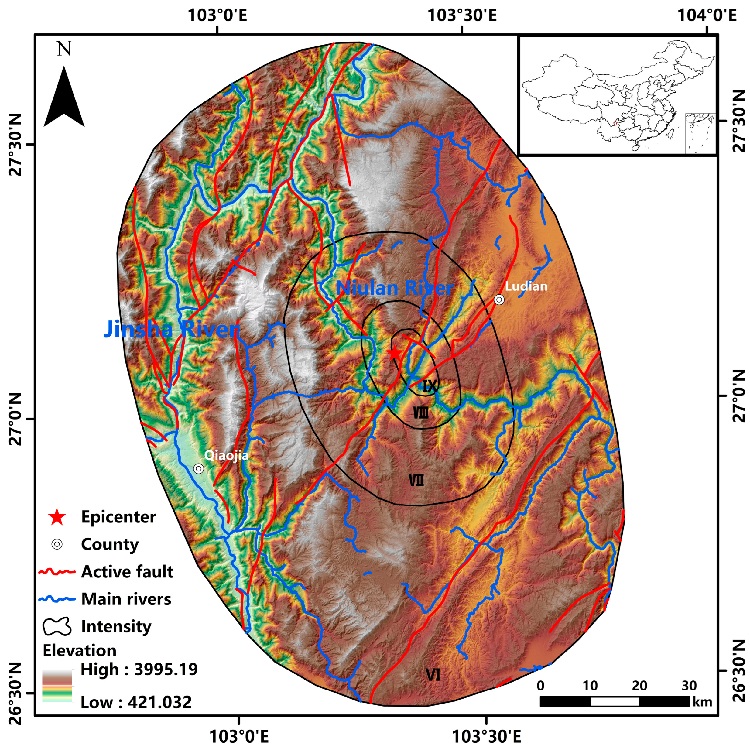
Figure 1. Map showing the location of the Ludian earthquake area (extent corresponds to the six-intensity zone, with the base map using ALOS 12.5 m DEM data).
Remotesensing 16 02951 g001
Figure 2. Map showing the seismic intensity distribution of Ludian earthquake (the source from the China Earthquake Administration, https://www.cea.gov.cn/cea/dzpd/dzzt/3571618/3571619/3577650/index.html), URL (accessed on 6 March 2024).
Remotesensing 16 02951 g002
Figure 3. Map showing the distribution of coseismic landslides induced by the Ludian earthquake (data sourced from [4]).
Remotesensing 16 02951 g003
Figure 4. Map showing the structural background of Ludian area in Yunnan province (BXF: Baogudang-Xiaohe Fault, ZLF: Zhaotong-Lianfeng Fault, SMF: Shimen Fault, LFF: Lianfeng Fault, JYF: Jinyang Fault, WLFF: Wulianfeng Fault, XJF: Xiaojiang Fault, ZMHF: Zemuhe Fault).
Remotesensing 16 02951 g004
Figure 5. Map showing the diagram of slope gradient growth and landslide erosion (revised from [24]).
Remotesensing 16 02951 g005
Figure 6. Map showing the schematic diagram of the process of calculating the excess topography (image modified from Blöthe et al. [29], (A) is original topography, (B) is threshold slope surface).
Remotesensing 16 02951 g006
Figure 7. Map showing the rock classification in the Ludian earthquake study area (adapted from the 1:500,000 Geological Map of China).
Remotesensing 16 02951 g007
Figure 8. Map showing the extraction results of excess topography in the Ludian earthquake study area.
Remotesensing 16 02951 g008
Figure 9. Map showing the development rates of seismic landslide areas in different excess topography intervals in the Ludian earthquake study area.
Remotesensing 16 02951 g009
Figure 10. Map showing the effective rock grouping in the Ludian earthquake study area.
Remotesensing 16 02951 g010
Figure 11. Map showing the distribution of slope in the Ludian earthquake study area.
Remotesensing 16 02951 g011
Figure 12. Map showing the landslide susceptibility distribution in the Ludian earthquake study area.
Remotesensing 16 02951 g012
Figure 13. Map showing the ROC curve analysis for the Ludian earthquake study area (The blue line represents the receiver operation characteristic curve, while the diagonal line indicates that the classifier has no discriminative ability.).
Remotesensing 16 02951 g013
Figure 14. Map showing the landslide susceptibility results referencing excess topography in the Ludian earthquake study area.
Remotesensing 16 02951 g014
Figure 15. Map showing the ROC curve analysis for the new landslide susceptibility in the Ludian earthquake study area (The blue line represents the receiver operation characteristic curve, while the diagonal line indicates that the classifier has no discriminative ability.).
Remotesensing 16 02951 g015
Figure 16. Map showing the PGA distribution for the Ludian earthquake event.
Remotesensing 16 02951 g016
Figure 17. Map showing the predicted earthquake landslide hazard under actual ground motion conditions in the Ludian earthquake study area.
Remotesensing 16 02951 g017
Figure 18. Map showing the seismic landslide area development rates for different hazard zones in the Ludian earthquake study area.
Remotesensing 16 02951 g018
Figure 19. Map showing the earthquake landslide hazard prediction based on basic ground motion conditions in the Ludian earthquake area.
Remotesensing 16 02951 g019
Figure 20. Map showing the distribution of coseismic landslides and earthquake landslide hazard under basic ground motion conditions in the Ludian earthquake area.
Remotesensing 16 02951 g020
Table 1. Critical slope values for different rock groups.
Rock GroupingHarder RocksSofter Rocks
Critical slope(°)3324
Table 2. Reference table for reduction factor.
Rock FormationReduction CoefficientDescribe
Carbonate rock formations1.0The lithology is mainly composed of limestone, crystalline limestone, argillaceous limestone, and dolomitic limestone, with locally interbedded quartz sandstone, calcareous quartz sandstone, shale, and sandy calcareous slate. This type of rock formation is generally dense and hard, often forming high mountain terrain with good mountain stability. The slopes are generally between 40–45 degrees and are prone to forming steep cliffs. From field investigations and existing data, it can be seen that the solubility of carbonate rock formations in the study area is not high. The reason for this is determined by the geographical location of the high mountains and cold regions where the study area is located, with only a small number of dissolution fractures visible.
Blocky hard rock formations0.9Mainly composed of intrusive rocks such as basic ultrabasic rocks of the Jinsha River ophiolite group, the rocks are dense and hard. However, due to the influence of structure, the rocks are fragmented, with developed joints and cleavage joints, resulting in a decrease in hardness. The main engineering geological feature of this rock formation is good stability. However, its weathering intensity has a significant impact on the physical and mechanical properties of the rock. The depth of the weathering zone in this rock formation is generally 3–15 m, with a fracture rate of 5%.
Layered hard rock formations0.8The lithology mainly consists of sodium feldspar chlorite schist, metamorphic diabase interbedded with Yangqi sodium feldspar quartz schist, mica quartz schist, quartzite, metamorphic sandstone, etc., mostly belonging to the category of hard or sub hard rocks. The main engineering geological characteristics of this rock formation are greatly influenced by their structures, with developed faults, cleavage, joints, and schistosity in the area. The rocks are fragmented, and there are significant differences in physical and mechanical properties, resulting in poor stability. Deep cut mountain areas are often formed on the terrain, which are the most severely affected areas for geological disasters such as landslides, collapses, and spalling.
Layered soft hard interbedded sub hard rock formations0.7Composed of various hard sandstones, moderately acidic volcanic rocks, limestone and mudstone, conglomerates, and interbedded pebbly sandstones, the rocks generally have strong cleavage, joints, and schistosity, and are highly permeable. The characteristic of this rock formation is a combination of “soft” and “hard”. Under the influence of engineering geological conditions such as high mountain deep cutting areas in the study area, the differential weathering is strong, and the stability of this group varies greatly. It is an unstable rock formation, often forming cliffs and steep walls, and is a prone area for geological disasters such as landslides, collapses, and peeling.
Scattered soft rock formations0.9These are composed of Quaternary floodplains, multi-level terraces, and slopes with sub sandy soil and crushed stone layers.
Table 3. Mechanical parameters of rock for effective grouping in the study area.
Effective Rock GroupingEffective Internal Friction Angle (°)Effective Cohesion (MPa)Unit Weight (kN/m3)
I33.00.17026.5
II23.10.11926.5
III19.20.08025.5
IV16.80.07025.5
Table 4. The Spearman’s correlation analysis between excess topography and critical acceleration in the Ludian earthquake study area.
Critical AccelerationExcess Topography
Spearman’s RhoCritical AccelerationCorrelation Coefficient1.0−0.771 **
Significance (two-sided) 0
N10,00010,000
Excess TopographyCorrelation Coefficient−0.771 **1.0
Significance (two-sided)0
N10,00010,000
** At the 0.01 level (two-sided), the correlation is significant.
Table 5. Potential landslide thickness in different excess topography intervals in the study area.
Excess Topography Interval (m)Average Excess Topography (m)Proportional CoefficientAdjusted Potential Landslide Thickness (m)
0010
0–51.4511.45
5–5022.810.12.281
50–10072.430.053.6215
100–250158.200.0253.955
250–500308.370.026.1674
>500517.780.0157.7667
Table 6. Corresponding values of seismic intensity and PGA in the study area.
IntensityVI (6)VII (7)VIII (8)IX (9)
PGA (m/s2)0.450–0.8990.900–1.7791.780–3.5393.540–7.079
Disclaimer/Publisher’s Note: The statements, opinions and data contained in all publications are solely those of the individual author(s) and contributor(s) and not of MDPI and/or the editor(s). MDPI and/or the editor(s) disclaim responsibility for any injury to people or property resulting from any ideas, methods, instructions or products referred to in the content.