Article

Summer Discrepancies between 2 m Air Temperature and Landsat LST in Suceava City, Northeastern Romania

by
Dumitru Mihăilă
1,
Petruț-Ionel Bistricean
1,*,
Lucian Sfîcă
2,
Vasilică-Dănuț Horodnic
1,
Alin Prisăcariu
1 and
Vlad-Alexandru Amihăesei
3,4
1
Department of Geography, “Stefan cel Mare” University of Suceava, 720229 Suceava, Romania
2
Department of Geography, Faculty of Geography and Geology, Alexandru Ioan Cuza University of Iași, 700506 Iași, Romania
3
Doctoral School of Geosciences, Alexandru Ioan Cuza University of Iași, 700506 Iași, Romania
4
Department of Climatology, National Meteorological Administration, 013686 Bucharest, Romania
*
Author to whom correspondence should be addressed.
Remote Sens. 2024, 16(16), 2967; https://doi.org/10.3390/rs16162967
Submission received: 14 June 2024 / Revised: 22 July 2024 / Accepted: 11 August 2024 / Published: 13 August 2024

Abstract

:
The widespread availability of Land Surface Temperature (LST) data from various sources presents a contemporary challenge for urban climate studies: how to efficiently compare these data with the results of traditional methods of temperature monitoring, which typically assume measurements at 2 m under sheltered conditions. In this line, the current study is based primarily on data extracted from a network of 31 points of hourly temperature monitoring at the 2 m level (Tair2m), in use between 2019 and 2021, in the city of Suceava in north-eastern Romania. These data allowed a detailed mapping for each hourly time step through multiple regression, adjusted by IDW, which was identified as the best interpolation method of Tair2m. These data were analyzed in parallel with LST data derived from Landsat imagery available in the analyzed period for 35 summer days with no or low cloud cover. The mapping results of both the Tair2m and LST data describe the main characteristics of the Suceava urban agglomeration (SvMA) heat island, which presents polynuclear features with intensities—as expressed by the temperature difference between the cores of the heat island and the surrounding rural areas—spanning during the summer noontime between 3.0 °C based on Tair2m and 7.1 °C on LST, respectively. The values of the Tair2m–LST differences were 0.68 °C on average, ranging from 5.33 to −19.17 °C, directly proportional to the imperviousness ratio (IMD) values, reaching the highest values in the local climate zones (LCZs) with a high built-up ratio (up to −19.17 °C) and the lowest (0.5 ÷ −0.5 °C) for those with bare soils, with isolated bushes and trees, with few or no buildings. The study results could serve as a tool to downscale the LST data to the level of Tair2m, which is useful for interpretation of the data derived from these commonly used tools in urban climate monitoring.

1. Introduction

Nowadays, the assessment of urban heat island extent and intensity tends to heavily rely on remote sensing tools, primarily for acquiring various Land Surface Temperature (LST) products, a practice that leads to an imbalance between urban heat island (UHI) evaluation methods. A major part of surface UHI (SUHI) studies based on remote sensing tools are currently developed on MODIS LST products [1] due to their high temporal resolution, but there are also other LST products that are extensively used in urban climate studies for their high spatial resolution, such as those from Landsat [2].
LST products play a pivotal role in urban climate assessment [3] as they offer a spatially detailed insight into the complex thermal environment of cities due to their high spatial resolution, and also extensive possibilities for use in connection with land cover [4]. It is generally well known that the LST is negatively correlated with the extent of vegetation cover [4,5] and positively correlated with built-up ratios [6]. Also, a high spatial resolution of LST, such as that from Landsat, offers the opportunity to assess in detail the impact of different types of land use in LST spatial variation, like the role of urban trees in the mitigation of LST increase [7], or that of dense urban fabrics [8]. The use of LST products is also very efficient in testing different urban solutions for mitigating UHI effects, such as high albedo impervious surfaces [9] or green spaces configurations [10]. Furthermore, previously, Landsat LST data have been used to suggest the best possible location of in situ urban weather stations [11].
In the meantime, the assessment of UHIs using in situ measurements—at 2 m above the ground and in sheltered conditions—has represented the classical scientific way to approach this topic, being enhanced nowadays by the increased accessibility to data loggers and progress in using crowdsourced data [12]. Moreover, currently it is considered that worldwide UHI mitigation relies strongly on software simulation, like ENVI-met, and remote sensing methods and, due to this, more attention should be given to field experiments or long-term weather observations [3]. Therefore, the use of in situ measurements in urban climate studies should be encouraged, especially due to the fact that they can offer a concrete image of the thermal comfort inside an urban environment [13].
In this context, there is a need to accurately analyze the differences between LST data and those resulting from in situ measurements [1]. This need is higher especially during the summer when heatwaves can amplify urban heat islands [13,14], and because the thermal environment of cities is more complicated, with large differences between the various types of thermal measurements. Moreover, the assessment of these differences is able to offer a detailed image of the urban thermal environment, through the combination of high spatial LST products and continuous observation from in situ air temperature measurements [15].
Consequently, LST products could represent a reliable proxy for in situ measurements of air temperature, both being linked by strong correlations, especially at the level of daily averages [16,17], even if in very large cities this correlation is weak [18]. Generally, the relation between LST products and Tair2m is dependent on the type of urban land use [19,20]. The positive differences between LST and in situ measurements are highest for the dense urban fabric, and negative especially for deciduous forest areas near cities [21]. Apparently, the colder and drier the city, the greater the difference between LST and Tair2m observations [22,23].
For the territory of Romania, studies on urban heat islands emerged simultaneously, based on remote sensing tools, using either MODIS [24,25] or Landsat [26], and direct in situ measurements [27,28], all being focused on Bucharest. Also, UHIs were extensively investigated for Iași, using both in situ measurements [29,30] and MODIS LST [15], the latter study including a detailed comparison between LST and Tair2m.
In this context, in some of these cities, relevant attempts have been made to investigate the difference between LST products and in situ measurements. These studies indicate that, in general, there is a good correlation between LST and Tair2m in the complex urban environment of Bucharest [31] and Craiova [32], especially during clear sky conditions [33]. For Bucharest, the difference between MODIS LST and Tair2m spans between 2 and 6 °C, with higher values in the central urban area with a high ratio of impervious surfaces and which is dominated by densely built-up land use types [34,35]. The same difference pattern, but with lower intensities (1–4 °C), was assessed for Timișoara [36,37] and Cluj-Napoca [38,39]. The differences between Landsat LST and Tair2m were found to be higher also in Bacău city [40], being ranged between 5.1 °C in an urban park environment and 7.1 °C in a densely built-up area, which is in line with the results obtained for numerous cities worldwide [41]. The use of a monitoring network for long-term observations of the Tair2m in Iași city showed that the differences between MODIS LST and Tair2m were higher than those from other articles [15]. This observation emphasizes the need for more extensive in situ monitoring networks to cover the wide variety of urban land use when assessing the differences between LST and Tair2m, to serve the scientific goals of urban heat island mitigation and adaptation [3].
The current study explores for the first time the characteristics of both the canopy layer (CLUHI) and surface urban heat island (SUHI) for the small city of Suceava, located in heterogeneous landform conditions in the north-east of Romania, enlarging urban climate knowledge beyond the mostly researched large cities [42]. The study pursues two main objectives: (1) to ascertain the characteristics of SUHIs by using Landsat LST data and those of CLUHI by using 31 Tair2m monitoring points during summer sunny days; (2) to assess for summer sunny days, the differences between the LST and Tair2m analyzed in relation to the impervious ratio, but also to urban land use conditions, as derived from the Local Climate Zones classification.

2. Materials and Methods

2.1. Study Area

SvMA is a territorially and economically dynamic urban agglomeration, and this dynamism is reflected in its local climate and microclimatic characteristics. The surveyed area covers 406.9 km2, in north-eastern Romania (Figure 1a,b), with altitudes between 249 and 530 m, with average values of 390 m. The Suceava river crosses the central part of the city for about 20 km, from NW to SE, splitting in two the analyzed territory (Figure 1c). The river meadow is unflooded and mostly used as an area for industrial or commercial use, and links the two main urban cores of the city.
In 2011, the entire SvMA had 140,488 inhabitants, and after the last census (2021), the population increased to 142,844 [44,45]. Within the administrative boundaries of the SvMA, from 2018, residential areas occupied 9.2%, industrial and commercial units 3.8%, agricultural land 48.6%, pastures and meadows 19.6%, forests 17.6%, and water areas 1.2% [46]. Comparison of the CLC 1990 [47] and CLC 2018 data shows that in this period the total area subject to changes represented 9.1%, with urban and industrial areas (including commercial complexes) having increased by 50.7%. Also, the construction and housing classes total area grew by 2.12% from the area of SvMA, with the largest part coming from arable land (1.86%).

2.2. Data

From the 31 monitoring points of Tair2m hourly observation data (2019–2021), originating mainly from a self-developed weather monitoring network, we extracted 35 hourly datasets corresponding to 11.30 AM Romanian time, in order to be synchronous with the crossing hours of available Landsat LST images (Table S1, Supplementary Materials).
Of the 31 observation points, one was represented by the Suceava official meteorological station (SMS) belonging to the National Meteorological Administration of Romania network, one by the meteorological station at Salcea airport (SAE) belonging to the ROMATSA network, and two other meteorological stations (SV1 and SV2) of the National Air Quality Monitoring Network, while the other 27 points were represented by meteorological posts installed by the USV team members involved in the current analysis (8 posts located in the Suceava municipality, 12 posts in peri-urban localities, 4 posts along the major Suceava riverbed and 5 posts in the urban and suburban forests—Table S2, Supplementary Materials). Based on this data, the canopy urban heat island (CLUHI) was assessed and discussed in our study.
The data used to generate the Landsat LST map model are summarized in Table 1.
The final LST map model based on Landsat data was generated by averaging 35 satellite scenes, of which 24 were Landsat 8 OLI&TIR and 11 Landsat 7 ETM+ satellite scenes, respectively. The satellite images were evenly distributed between the summer months, with 12 images from June, 10 images from July and 13 images from August (Table S1). Due to the importance of cloud cover in shaping UHI characteristics [49], but also taking into consideration the high level of cloud cover in Suceava, drastically restricting the number of possible Landsat LST scenes, we decided to select for our analysis only images with less than 50% cloud cover, while the values for missing pixels were filled using the DINEOF method. Based on Landsat LST data, we assessed the surface urban heat island (SUHI) as presented and discussed in the study’s results.
Furthermore, ASTERGDEM [50] was used as the digital elevation model, and was also used as the source for the altitude, slope, and exposure measurements used in the multiple regression analysis.

2.3. Methods

2.3.1. Gap Filling of Land Surface Temperature

The Data Interpolating Empirical Orthogonal Functions (DINEOF) method was used in this study as it has been shown to be more efficient than geostatistical methods (e.g., interpolation, empirical regression) in filling missing data in LST products, yet requiring less data input and less computation time [51]. The DINEOF method uses spatio-temporal patterns in the data in order to predict what the missing values should be. Firstly, the images in the time series are converted into a matrix whose columns represent the image pixels recorded at the same time, while the rows represent the different times of recording (days). Next, the DINEOF algorithm decomposes the time series into a set of orthogonal functions well known as empirical orthogonal functions (EOFs) [52]. These EOFs capture the dominant patterns of variability in the data. Then, DINEOF uses the EOFs to reconstruct the original time series but replaces missing values with estimates based on the patterns in the data. The final step is to combine the reconstructed time series with the original data to create a complete time series with no missing values. In previous studies, the DINEOF method has been successfully applied to the reconstruction of sea surface temperature [53,54] or in mountainous regions [51]. Cheval et al. [55] also used the same method to fill Landsat LST images for Bucharest and [56] applied the method for MODIS data in Bacău city. DINEOF proved to also produce good results as a gap-filling technique for Landsat LST (RMSE < 2, R2 > 0.7) for the most important cities in north-eastern Romania [57]. By employing DINEOF, the gaps in the LST data resulting from limited cloud cover were effectively filled, enhancing the overall data completeness and reliability. The DINEOF gap-filling method for a gridded dataset was implemented using the “rtsa” library [58] developed in R [59].

2.3.2. Interpolation of Tair2m Data

In the first phase, for the spatial interpolation of the Tair2m data, we tested the performance of five spatial interpolation methods: simple regression, simple regression adjusted by ordinary kriging, simple regression adjusted by IDW, multiple regression adjusted by ordinary kriging, and multiple regression adjusted by IDW. In order to assess the performance of each method and to choose the best one of them to work with in the following phase, from 31 monitoring points, we randomly left out six of them (NOV, IPT, SFI, ZAM, APD, VRT), performing the interpolation with the other 25. After that, the mean values of these six points were compared with the values extracted for each point from the maps of the interpolated methods used, the best method being considered the one with the lowest deviation from the measured value (Table 2). Analyzing the obtained results, the method with the best performance was the interpolation of the Tair2m data by multiple regression adjusted by IDW. This method gave estimated values with the minimum deviation for the six left out points (Figure 2) with a mean deviation of 0.68 °C.
At the end of this process, the Tair2m from the 31 chosen points of observations corresponding to the times of the satellite passing over Suceava were interpolated through the selected method. The multiple regression integrated parameters, such as the altitude, inclination and slopes exposure, and the general model obtained was the following:
Y = (−5.1976 × Xalt) + (−0.5856 × Xslo) + (−13.221 × Xexp)
where Y = Tair2m from the local hour corresponding to the satellite scenes crossing time from the summer months (2019–2021), Xalt = the altitude of each meteorological observation point for the in situ monitoring network, Xslo = the slope that shows the DEM inclination of the pixel in which the observation point was located, and Xexp = the slopes exposure, which shows the exposure in relation to the sunlight/air circulation of the pixel in which the observation point was located.
Firstly, from the numerical model of Tair2m obtained by multiple regression, the values based on the 31 monitoring points were extracted. Thereafter, the differences between the actual thermal values obtained from the measurements and those estimated by multiple regression were calculated. The spatial pattern of these differences interpolated by IDW was added to the pattern estimated by multiple regression, resulting in the final map of the spatial distribution of Tair2m in SvMA for the 35 selected time steps.
It should be noted that the resolution of the rasters in this study was 30 × 30 m, identical to that of the Landsat LST satellite images. This was obtained by using available ARCGIS tools for resampling the spatial data.

2.3.3. Methods for Ancillary Remote Sensing Data Treatments

Kernel Density (KDE) of Impervious Density (IMD) for 2018

In order to understand how urban land use influences the differences between Tair2m and Landsat LST values at a local level, we used IMD values data taken from Copernicus [60]. The assessment of these parameters was made by using ArcGIS 10.8. Firstly, the raster image of the IMD was converted into points by using the “Raster to Point” function from the “Conversion Tools” function. The resulting points were interpolated using the “Kernel Density” function from the “Spatial Analyst Tools” toolkit. This function calculates the density of each point in a vicinity around each output raster cell with a resolution of 1000 m. During this process, a smoothly curved surface (kernel surface) is fitted over a circular vicinity of each point based on the quartic kernel function [61]. The surface value is the highest at the point location and decreases at the same time with increasing distance from the point, reaching zero at the boundary of the circular proximity. Subsequently, the raster was reclassified into 10 classes ranging from 0 to 100%, by a similar method to [62].
The grid network was designed by using the Fishnet tool function in ArcGIS V10.8, having a square size of 500 × 500 m, in order to correspond with the spatial resolution of Landsat LST. We chose to create centroid points for each square from the network by using the “label points” option from the Fishnet tool. The distance between points was 500 m, resulting in a grid network of 1626 points. The resulting points were used to extract the temperature values (Tair2m and LST), IMD, and other input data for the Digital Elevation Model, enabling the organization of a detailed statistical database.

Local Climate Zones (LCZs) Classification

To highlight the influence of the land use pattern, especially in the urban environment, Ref. [63] proposed a classification of the urban landscape intended to take into account the land cover and its physical properties. By using the LCZ classification, which is a typical classification scheme for urban surface temperature [3], we aimed to obtain not only a local, as given by IMD, but a wider image of the differences between LST and Tair2m in relation to different types of urban land use.
The characterization of the urban landscapes was achieved by classifying the urban area into areas of uniform land use, with structure, materials, and human activities specific to them, called LCZs. For the generation of the LCZs, a so-called training file was created, in which, based on Google Earth images, between 5 and 10 areas from within the SvMA for each class were determined. The LCZ Generator application (developed on the WUDAPT platform) extracted from Landsat 8 satellite imagery the features of the urban surface and classified them into 17 classes. From these, 10 classes were determined on the basis of the building types and 7 classes on the basis of the land cover [64].
The generation of SvMA-specific LCZs resulted in the identification of 9 classes in the category of defined building types and 7 classes in the category of land cover. Due to the relatively small extension of the analyzed region, we manually improved the LCZ classes delimitation. Therefore, the degree of accuracy of the SvMA territory analysis is very good. Given that the maximum accuracy value is 1, the following levels of accuracy were obtained for this analysis: overall accuracy—0.83; accuracy for urban LCZ classes—0.75; overall accuracy of built/natural LCZ classes—0.97; weighted accuracy (OAw)— 0.96.
With reference to the classifications performed by [63,64], the following classes were identified within the SvMA according to the type of construction: class 1—tall buildings; class 2—compact, medium-sized buildings; class 3—compact, low buildings; class 5—isolated, medium-sized buildings; class 6—low, isolated buildings; class 7—light, low buildings; class 8—extensive, low buildings; class 9—lightly built-up areas; and class 10—industrial areas. It should be noted that, for class 4 of the classification (tall, detached buildings), no areas with these characteristics were identified within the SvMA. The land cover pattern generated the following surface types: A—densely wooded areas; B—areas with scattered trees; C—shrubs; D—low plants; E—paved areas; F—bare ground or sand; and G—water. Of these, in the SvMA, the highest proportion is of areas covered with herbaceous plants or agricultural crops (52%), and the lowest is of areas with sandy or unvegetated areas and land on which tall buildings stand (0.02%) (see Figure 3a–c).
The network of meteorological and thermal monitoring points operating for 3 years in the field (2019–2021) sampled more than 50% of the LCZs related to the urban agglomeration, the peri-urban, and the rural environment (Figure 1 and Figure 3c).

3. Results and Discussion

3.1. Thermal Differences Results between Tair2m and Landsat Surveys

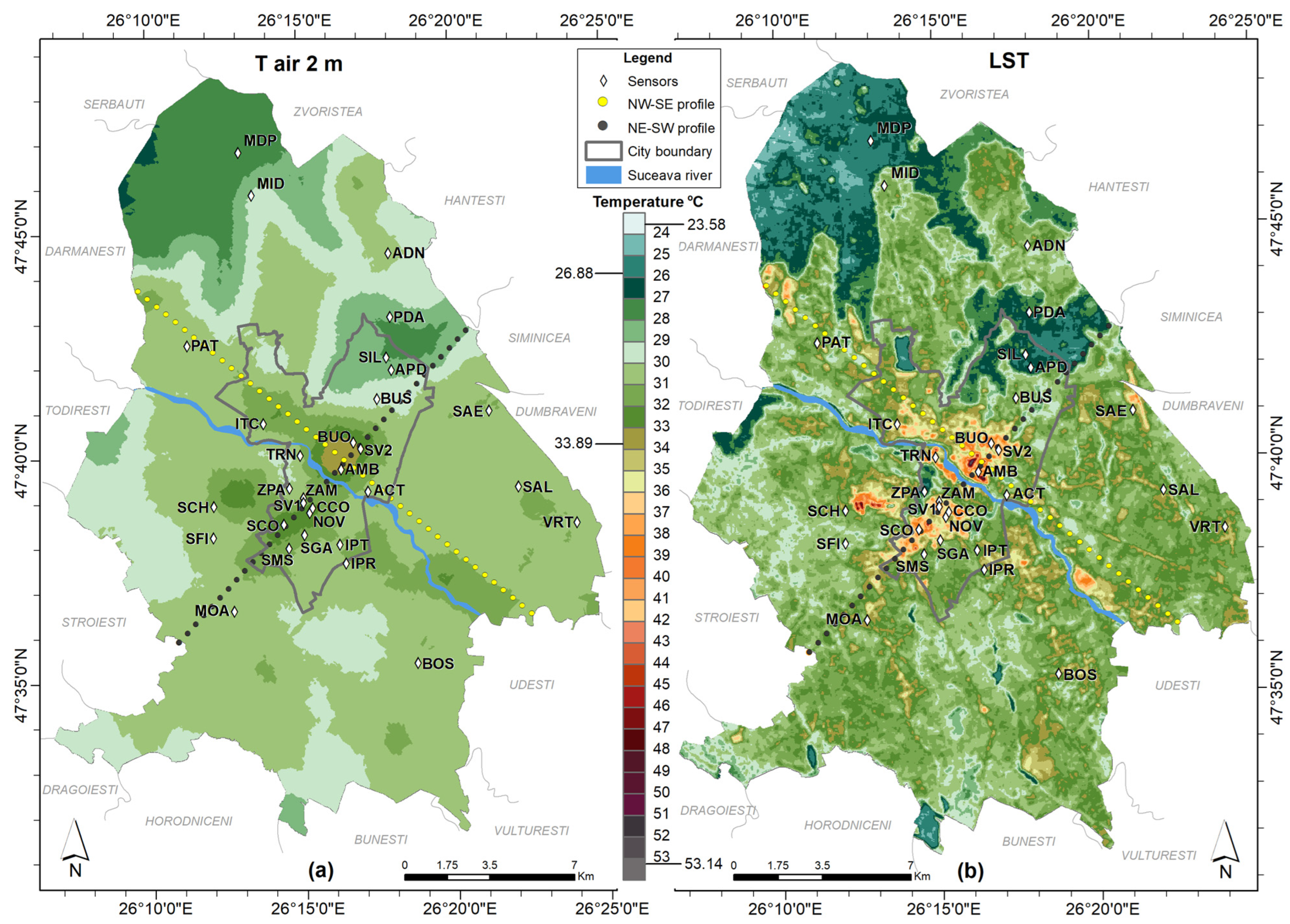
Our analytical approach integrates field observations with remote sensing [1,65]. As a general feature, the more complex typology of the topographic surface in cities, in which many anthropogenic composite materials are used (concrete, asphalt, sheet metal, etc.), induces a higher variability in the spatial distribution of LST than in the case of the 2 m level in air. The analysis of the two map representations (Figure 4a,b) allows the identification of the areas with the highest temperature values, which in both cases (Tair2m and LST) highlight the polynuclear urban heat islands. For CLUHI, as indicated by Tair2m (Figure 4a), a thermal average of 29.4 °C, a minimum of 26.9 °C, and a maximum of 33.9 °C were identified, while for SUHI, as indicated by LST (Figure 4b), an average of 32.7 °C, a minimum of 23.6 °C, and a maximum of 53.1 °C were observed. Obviously, territorial thermal extremes are more attenuated on the Tair2m map (7.0 °C) and more accentuated on the LST map (29.6 °C).
Based on the mean Tair2m distribution for the 35 selected days, it is assessed that the summer CLUHI in Suceava has several cores during the daytime. A first core is positioned over the Burdujeni urban neighborhood in the north-east of the city, with extension through the areas with railway infrastructure towards the Ițcani neighborhood located in the north, but especially towards the industrial platform and nearby commercial areas located in the Suceava river meadow. The heat island thins out in the sector of the major bed of the Suceava River and extends to the SE of it in the neighborhoods around the historical center of the city, located on the terrace on the right side of the Suceava River with connection to the peri-urban locality of Șcheia. In this extension, the CLUHI is bounded by the 31 °C isotherm, and at its hottest points, Tair2m exceeds the 33 °C threshold.
In contrast to the CLUHI, within the SUHI, we can identify with great clarity as cooler environments, the forests around Suceava (Adâncata, Mitocul Dragomirnei, Pătrăuți, Mihoveni) and the urban forests Șipote and Zamca, where the LST values drop below 28 °C (Figure 4b), underlining the efficiency of these land cover types in UHI mitigation [7]. The territorial distribution of LST spans over a wider range of values than the Tair2m and includes more spatial details. The SUHI is territorially more extended and better expressed, being delimited by the 33 °C isotherm, with the 35 °C isotherm delimiting large areas in the core of the city. Moreover, the built-up, heavily anthropized areas are the warmest, exceeding 40 °C in several places, and even 50 °C in some points. These results correspond broadly to those obtained for Iași, where the SUHI for the summer season is bounded by the 35 °C isotherm [15] and confirms the high intensity of SUHI during the day assessed using MODIS LST by [33]. On the LST map for Suceava, several hotspots stand out: the runway of the “Ștefan cel Mare” Airport in Salcea, the platform of S.C. Termica S.A. and Bioenergy S.R.L., and the industrial-urban infrastructure of the peri-urban locality of Șcheia. The areas covered with forest vegetation and those covered by water bodies are outside of the 30 °C isotherm, being distinctly visible on the LST map (Figure 4b). Cold spots appear within them and the LST also falls below the 25 °C threshold even during the analyzed summer sunny days.
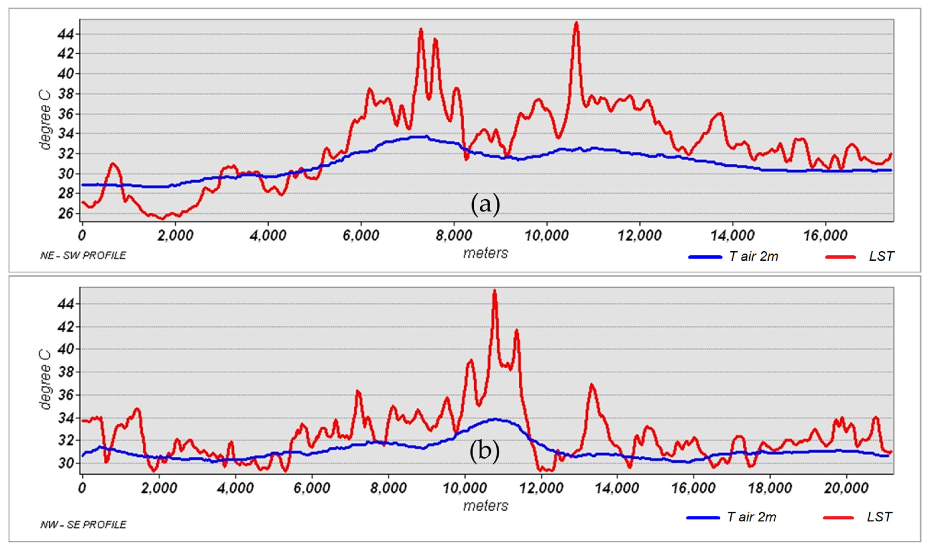
The thermal profiles of Tair2m and LST through the NE–SW direction, beyond the higher variability of the LST profile, show very clearly the positioning of the main CLUHI and SUHI nuclei above the Burdujeni neighborhood, the decrease in their intensity above the major riverbed of the Suceava river, and the regeneration, to some extent, of the CLUHI/SUHI intensity above the urban neighborhoods located on the structural plateau of Suceava (Centru, Mărășești, Areni, George Enescu, Obcini) (Figure 5a). These profiles also underline the very complex role of landform diversity for the characteristics of the UHI [66].
The thermal profile in the NW–SE direction on the Tair2m map passes through the central part of the CLUHI and has a more orderly, but also more valorically attenuated, course than the same profile conducted on the SUHI through the LST thermal field (Figure 5b).
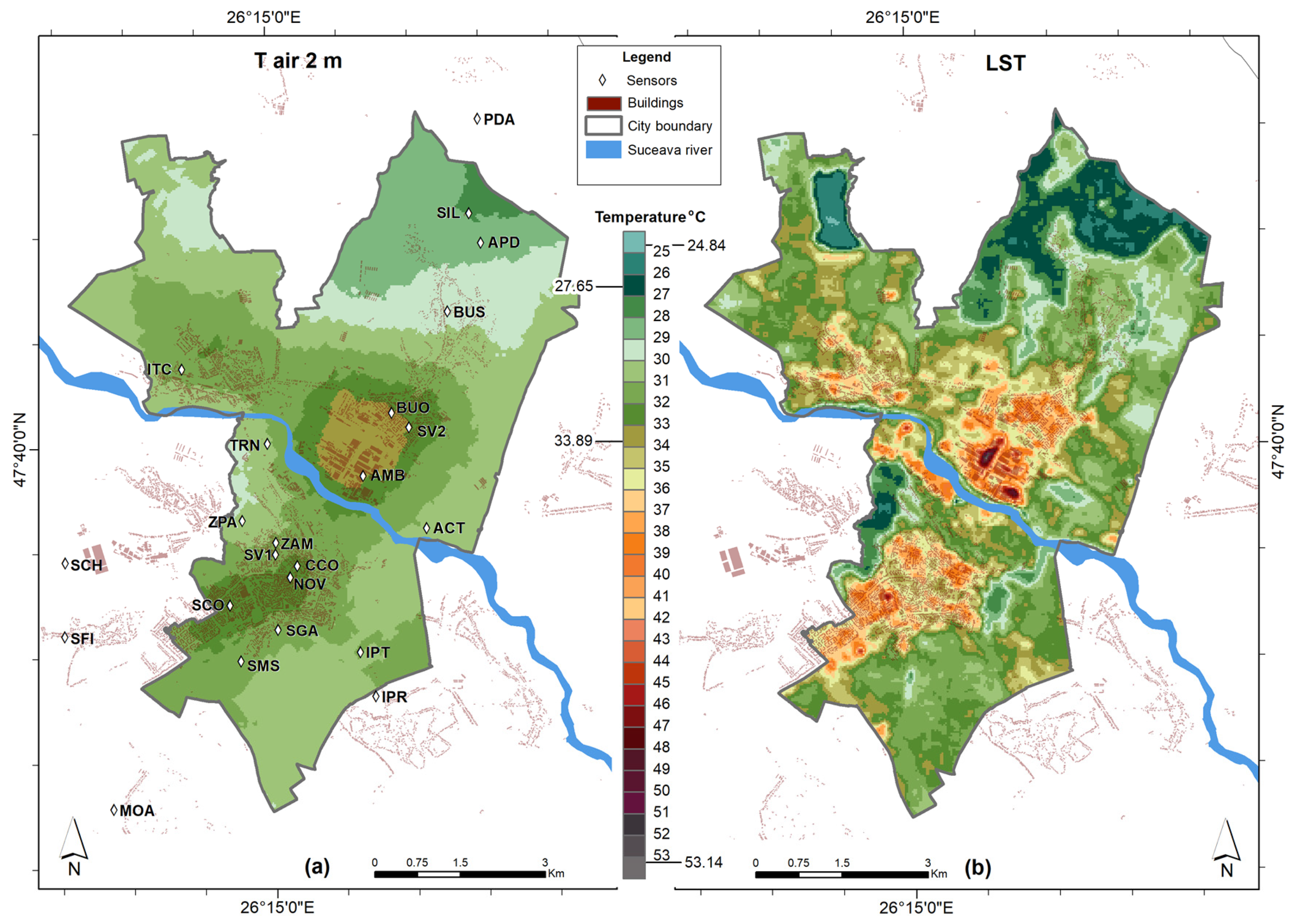
The details of the territorial footprint of the CLUHI and SUHI in Suceava city area are well expressed in Figure 6a,b. If we added the peri-urban locality of Șcheia, we would notice that the CLUHI, delimited on the outside during summer mornings by the isotherm of 31 °C, is formed by four nuclei. We distinguish the first one by its intensity and magnitude, including the Burdujeni neighborhood, the industrial platform and the commercial area of Suceava, with the in situ monitoring points BUO, SV2, and AMB. The second core is located in the flat part of the city, with the neighborhoods Centru, Areni, Mărășești, George Enescu, and Obcini (points CCO, NOV, SCO), while a third one extends above the peri-urban locality of Șcheia (SCH—more visible in Figure 4a). The last CLUHI core, more blurred and most probably on the increase, in the Ițcani neighborhood (ITC), seems to be imposed by the thermal imprint of the urban-rail infrastructure.
The Zamca Urban Forest (ZPA) and the major riverbed of Suceava have the potential to interrupt the territorial continuity of the CLUHI, to fragment it, and to diminish its intensity. The spatial distribution of SUHI nuclei (Figure 6b) overlays the hottest areas of Suceava, represented by the parking lot and the Leroy Merlin Carrefour, Dechatlon, and Egros shopping stores, respectively, and the parking lot and the commercial spaces of the Iulius Mall Suceava shopping complex, where the LST values exceed the 45 °C threshold at noon. Some parts of the Adâncata Forest, the Zamca urban forest, and Lake Dragomirna appear instead clearly on the LST map as colder areas (below 27 °C). CLUHI and SUHI (Figure 6a,b) show many similarities in terms of the temperature distribution, but the differences between them are also visible, due to the higher level of detail of the hot and cold, well expressed on SUHI (Figure 6b). At Suceava, the SUHI–CLUHI difference is, on average, 2–5 °C, while at Iași (daytime, summer), according to [15], this is 5–7 °C.
Tair2m in those 35 sequences related to the satellite passage over SvMA (which occurred for the satellite scenes used between 8.05 and 9.08 GMT hours, 11.05 and 12.08 official time; 3 + GMT according to Romanian summer time) was 29.4 °C on average, and the LST derived from Landsat imagery was 32.7 °C, resulting overall in a Tair2m–LST thermal difference of 3.3 °C. The thermal differences between Tair2m and LST are almost zero or very low on the lands with a low degree of built-up area, which do not have very steep slopes and are used as agricultural land (arable, pasture, meadow). For this type of land, the Landsat LST could be used easily as a proxy for Tair2m. On the lands covered with forest vegetation instead, those with an excess of moisture or water and the ones with a strong inclination of the slopes and with a generally northern exposure, the Tair2m–LST difference indicates positive values (+5.3 °C) before midday of the summer sunny days, indicating a slight thermal advance in the air compared to the level of the topographic surface.
The largest differences between Tair2m and LST are reached in areas with a high impervious ratio, covered with composite materials with different thermo-caloric capacities and conductivities, with surfaces with different albedo values, slopes and exposures, with the latter thermal parameter, as can be seen in Figure 7, being able to exceed the former by 5 to 20 °C. Similar results were obtained for Cluj by [67], and for Bucharest by [26] and underline the complexity of thermal conditions near the ground inside urban areas [68].
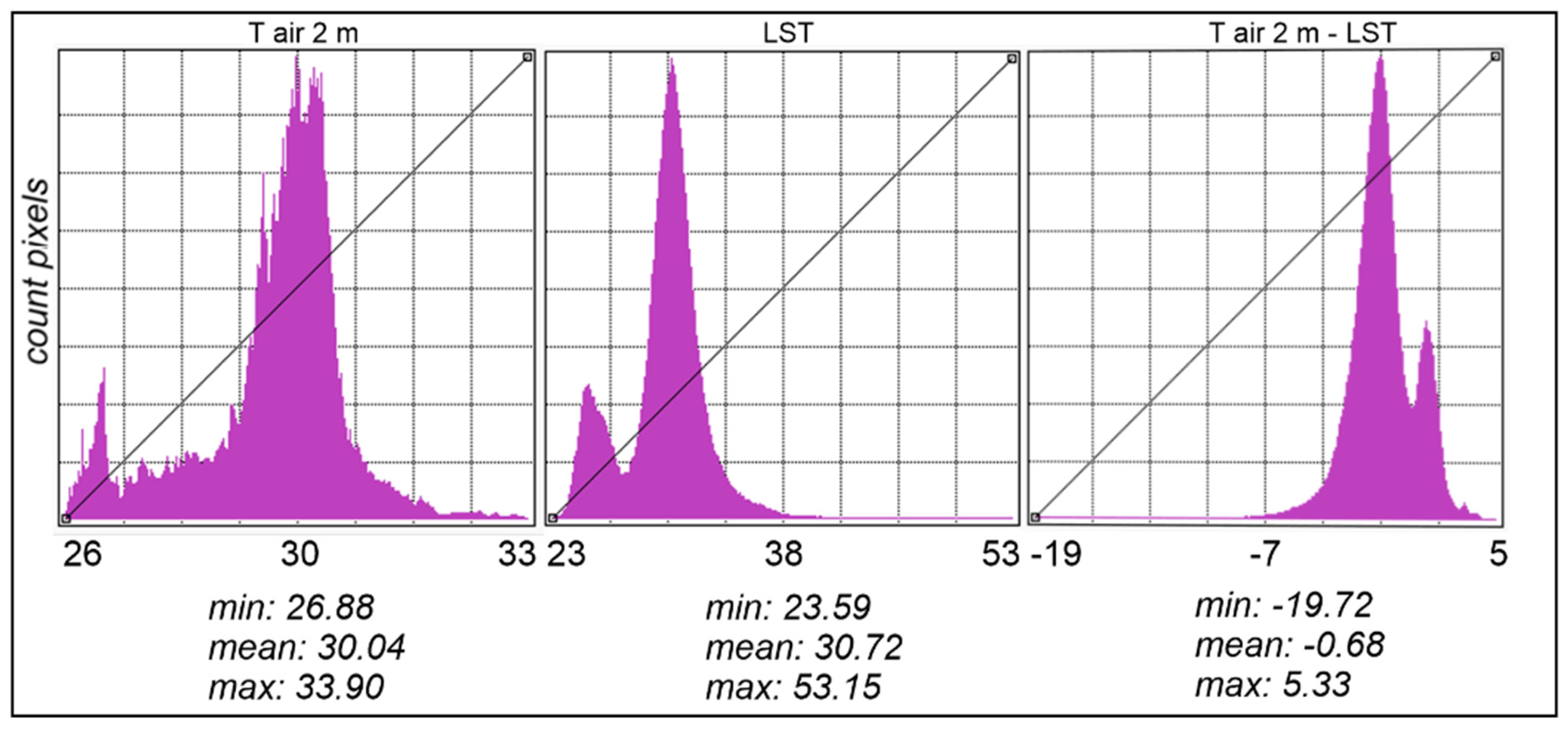
By analyzing for the whole area of SvMA the frequency histograms for the Tair2m, LST, and the Tair2m–LST differences (Figure 8), it is observed that the Tair2m values on the SvMA decreased to 26.9 °C, and had an average of 30.0 °C and a maximum of 33.9 °C, while the LST values decreased to 23.6 °C, had an average of 30.7 °C and a maximum of 53.2 °C. The Tair2m–LST histograms show larger differences in some specific situations in the city: (i) red hotspots (Figure 7) in the case of LST up to 19.7 °C higher than Tair2m, but values between 7 and 19.7 °C occur only occasionally; (ii) on average on SvMA, the temperature values are 0.7 °C higher for LST than Tair2m and; (iii) in the areas with forest vegetation, the Tair2m values can even be 5.3 °C higher than LST. Actually, LST with values >35 °C delimits the summer SUHI during the day also in Cluj-Napoca [67], and in Bacău [56]. Due to its higher altitude or reduced size, the central area of Suceava is also delimited by the 31 °C isotherm. In Galați, according to [69], the heat island of the city is binuclear, but in Suceava, it is made up of four nuclei.
While Ref. [18] or Ref. [70] did not succeed in finely correlating the Tair2m with LST in their studies, similar to Ref. [21], Ref. [22], or Ref. [23], we, in the present study, obtained small mean differences between the two thermal parameters. On average, the Tair2m–LST differences for the abovementioned authors fell within the limit of −8.5 °C, while ours were −0.7 °C, this being explained by multiple factors. Firstly, compared with other large cities, Suceava city reflects the characteristics of CLUHI and SUHI in small cities. Secondly, our results indicate the thermal conditions during the first half of the sunny summer days, with the extended urban surface remaining colder (LST) after the night when compared to the air near the ground (Tair2m), leading overall to mean differences close to 0 °C (−0.68 °C). Nevertheless, some patches of artificial surfaces are warming up very rapidly causing the very high values of LST indicated by the negative values in Figure 7. In fact, these last areas play the major role in the development of the SUHI during the day that is propagated also in CLUHI development in the afternoon hours and its peak during the night in summer [29].
From this perspective, our results validate previous results for Romanian cities, where the LST–Tair2m correlations are high [31], and relatively similar to those obtained for Bucharest [34,35], where the difference between LST–Tair2m has values of 2–6 °C, including Timișoara, with values of 1–3 °C [36,37], and Cluj with values of 1–4 °C [38,39], while for Craiova [32], the LST/Tair2m correlation indices have values between 0.77–0.83. For an urban park in Bacău, [40] determined LST–Tair2m differences of 2.5 °C. The authors of [33] found, for cities in Romania with more than 30,000 inhabitants, good correlations between LST and Tair2m in summer, during the daytime and in clear weather.

3.2. Thermal Differences between Tair2m and LST Conditioned by the Imperviouss Density

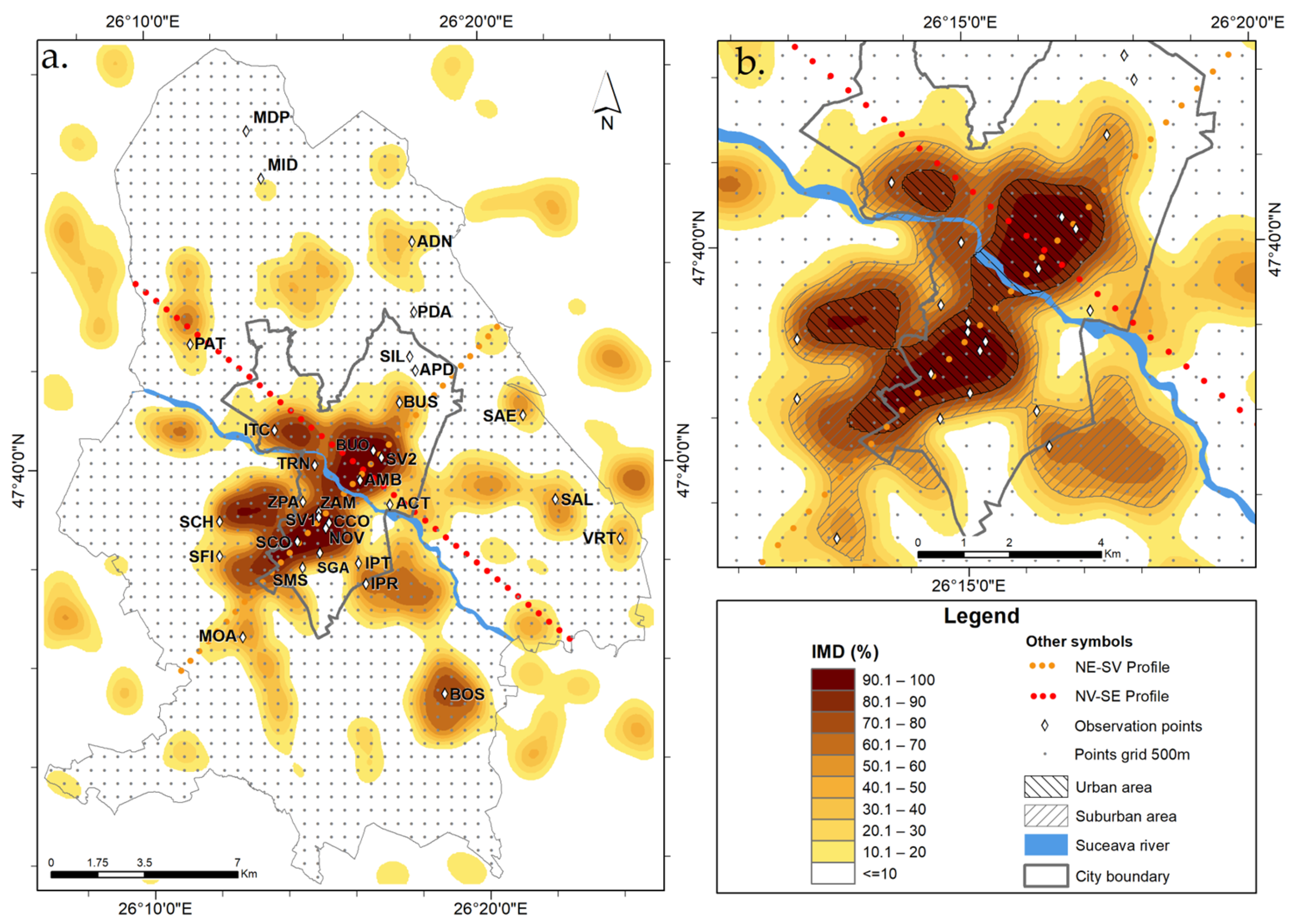
In our analysis, we regarded as urban the area where the IMD is higher than 80%, as peri-urban, the area where the IMD is between 40 and 80%, while IMD values below 40% were considered as rural areas (Figure 9 and Table 3). Other researchers have also used this index with good results in studies of this kind [56]. The analyses of Figure 9a for SvMA and of its detail focused on the Suceava municipality (Figure 9b) allow us to identify in the IMD distribution the same four cores which appear both on the Tair2m maps (Figure 4a and Figure 6a) and on the LST maps (Figure 4b and Figure 6b). These hotspots are clearly distinguishable in Figure 4b and Figure 6b and, by their specific features, the negative differences with values below −10 °C (but not lower than −19.72 °C between Tair2m and LST).
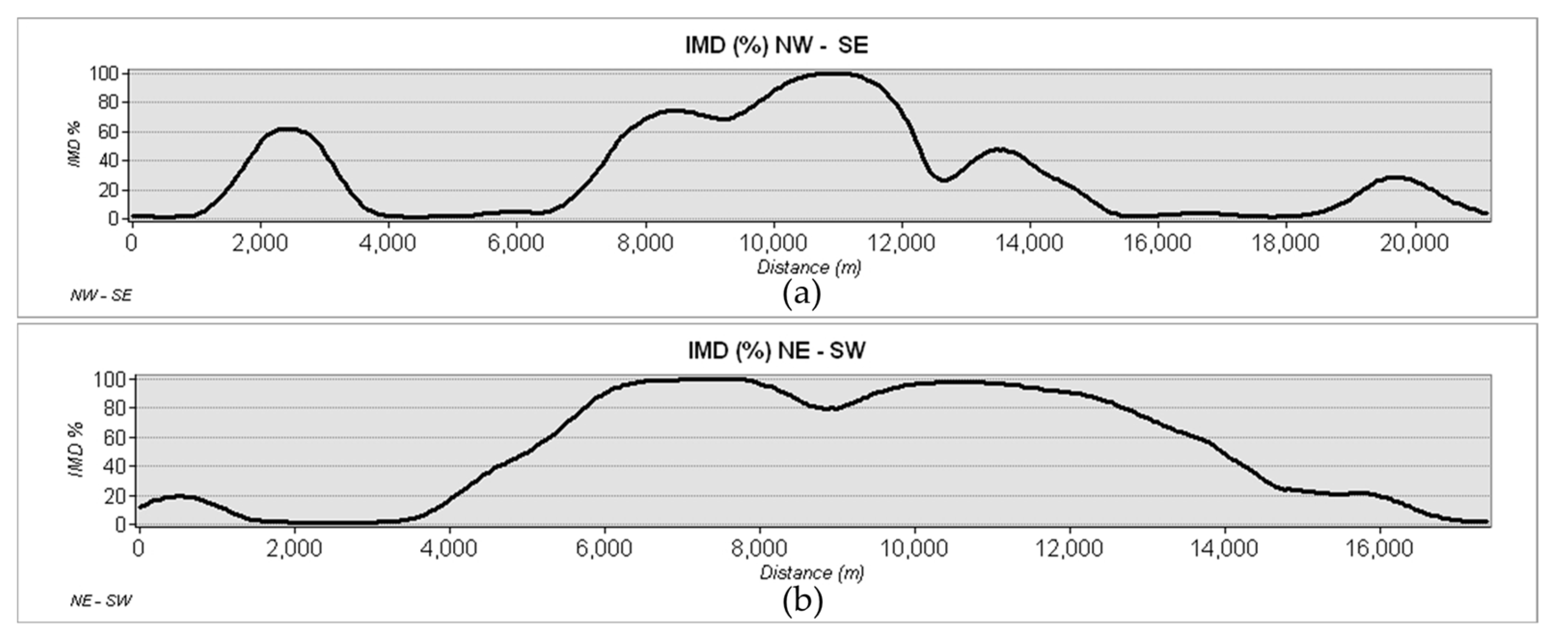
The profiles of the IMD value field in SvMA capture the areas with a dense urban infrastructure above which there are ideal conditions for CLUHI and SUHI development (Figure 10a,b).
The UHI appears polynuclear, where the density of the continuous urban infrastructure expressed through the IMD is higher than 80%, with a length of more than 6 km on the long axis (NE-SW) and 2.5–3 km on the short axis (NW-SE) (Figure 10a,b, respectively).
According to the statistics of this study, the thermal differences between the urban areas and the peri-urban areas is of 1.2 °C for mean Tair2m and of 3.2 °C for the LST, while the difference from the rural area is of 2.3 °C for Tair2m averages and of 5.4 °C for the LST (Table 3). These differences also represent a good proxy of the CLUHI and SUHI intensities, confirming that an impervious surface can be used as an explanatory variable of the UHI intensity [71]. The average differences between Tair2m and LST at the analyzed hour fade as the degree of anthropization of the topographic surface decreases, being −3.6 °C in the urban area with IMD > 80%, −1.6 °C in the peri-urban area, with IMD between 40–80%, and only −0.5 °C in the rural area with IMD below 40%. The differences with a negative sign indicate that at the time of the satellite passage over SvMA, the Tair2m is lower than the LST, which is similar to the results shown in Figure 7 and Figure 8.
For the maximum temperature values, the Tair2m–ST differences are the largest in value. In the urban and peri-urban areas, where those hotspots occur, LST can be higher than Tair2m, with values ranging between 12 and 19.3 °C before noon, and in the rural areas, the differences fade down, decreasing to 7 °C (Table 3).
If we take into account this thermal reality given by the differences between the thermal parameters of Tair2m and LST (Table 3), in future, we can use the satellite images converted for thermal analysis of the urban environment of SvMA even in the absence of some points of in situ meteorological measurement.
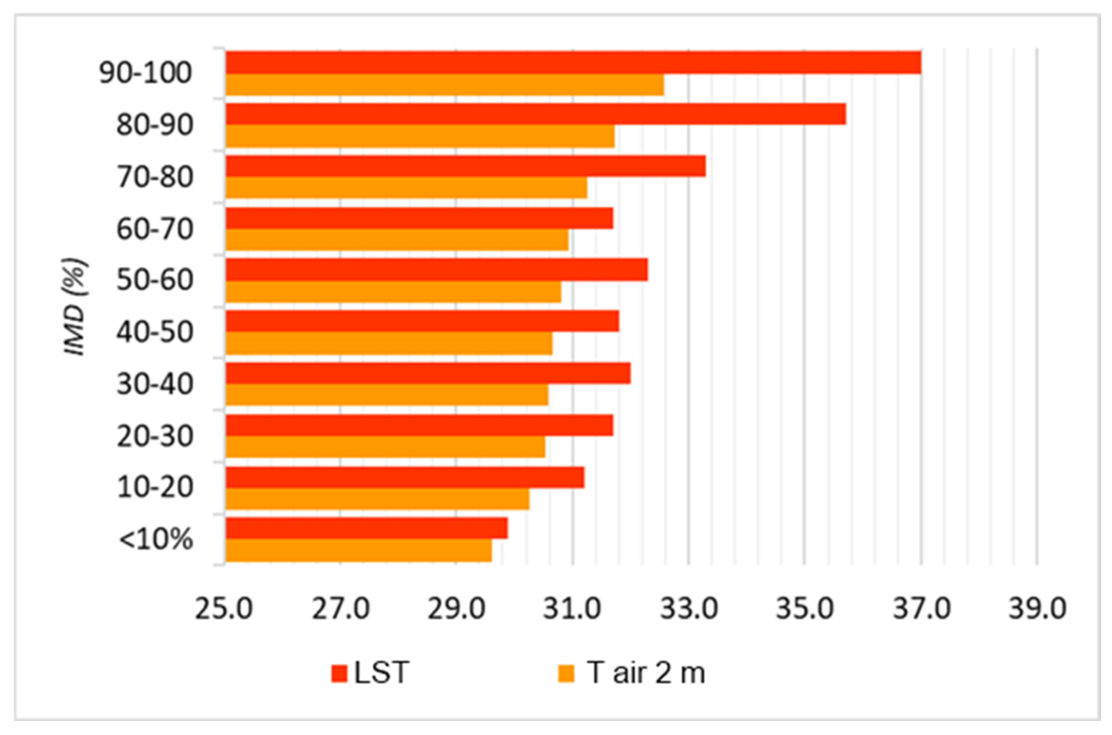
By analyzing the thermal characteristics for different thresholds of the IMD for Tair2m and LST, detailed for the 1628 grid points that covered the SvMA area (Table 4), we can see that the UHI, expressed as the difference between the mean temperature of areas with IMD < 10% and areas with IMD > 90%, reaches an intensity of 3.0 °C for Tair2m and by 7.1 °C for LST.
The differences between the Tair2m and LST averages are negative in the urban environment (−4.0 to −4.4 °C) towards the midday of summer days, when the urban surface becomes warmer than the air environment at 2 m level. For the rural environment, the Tair2m–LST differences are maintained between −0.3 and −1.4 °C. Overall, the obtained results offer support for the use of Landsat LST data as a proxy for Tair2m and vice versa for summer noon days. In the peri-urban environment, the Tair2m–LST differences are also negative and increase slightly in value compared to the rural environment, ranging between −1.2 and −0.3 °C. For minimum values, for all IMD classes, the thermal positive differences between Tair2m and LST are not very high (between 0.2 and 3.6 °C). By analyzing Tair2m–LST, for the maximum values of the differences, we found that in the peri-urban environment (IMD 40–80%), they have the lowest values (−3.5 to −4.5 °C); in the rural environment (IMD < 40%), the differences increase, especially above the exposed arable land with low slope and generally south-facing chernozemic soils, ranging between −3.3 and −6.4 °C. The differences in the Tair2m–LST maximums are maintained as a negative sign and reach the highest values in urban areas with IMD > 80% (from −11.2 to −12.4 °C) due to their particular profile and structure.
The distribution of the Tair2 m and LST values on different IMD thresholds above SvMA unequivocally indicates an increase in their differences as the IMD values increase (Figure 11). After establishing the spatial and temporal pattern of these differences, the two ways of exploring the temperature at different levels of those urban environments can be complemented one by the other.
Based on our results, we reach the conclusion that LST products, such as Landsat in our study, can be used as proxy data for Tair2m observations, having as a key control the differences between them filtered through the IMD ratio, which is by far the main control factor of the observed differences.

3.3. Thermal Differences between Tair2m and LST Conditioned by LCZ

We enlarge the understanding of the role of the built-up ratio on the magnitude of the differences between Tair2m and LST from a local level, as indicated previously by IMD, to urban land use types, as indicated by LCZs. The majority of the in situ monitoring points (11) belonged to LCZ 6, followed by highly urbanized LCZ 1–5 with nine monitoring points. Also, one monitoring point is located in each of LCZ 7–9. Furthermore, LCZ A indicating forested areas sum up five monitoring points, while LCZ D, that is mostly agricultural land, is covered by the other three monitoring points. Generally, we notice that these 31 points physically cover most of the LCZs identified and can be subjected to an analysis of this type. Across all LCZs, Tair2m–LST has a minimum value of 3 °C, an average of 1.8 °C, and a maximum value of negative sign (−19.3 °C), as indicated in Table 5.
By analyzing Tair2m–LST based on average values, we observe that the highest negative differences (between −6 and −3.9 °C) are specific to LCZ 1–2 (densely built-up areas), and LCZ 8–10 (industrial use). It is obvious that the heavily anthropized areas have average values of the LST higher than those of the Tair2m. Refs. [41,72] noted that the highest LST values are in the built-up LCZs, and [17] noted that in the densely built LCZs, the LST is 6.7 °C higher than in the natural ones. The lowest values of the Tair2m–LST difference (between −0.5 and 0.5 °C) are specific to LCZ F, LCZ B, LCZ C, representing land use types that are specific to rural and peri-urban areas.
The highest average values (1.6–1.8 °C), of positive sign, of Tair2m–LST are specific to classes A (densely forested areas) and G (water), which at noon of summer days at the 2 m level, is warmer than at the level of the emissive surface.
The highest values of the differences (−16.0 ÷ −19.3 °C), of negative sign, of Tair2m–LST were recorded above classes E (paved areas) and 8 (extended, low buildings).

4. Conclusions

In our study, we have shown that, at least for small and medium-sized cities, such as Suceava, Landsat LST data could complement air temperature in situ measurement and both can be used in climatic studies in a complementary way. Our results show, firstly, that during the summer noon, the CLUHI of the Suceava urban agglomeration is delimited to the exterior by the 31 °C isotherm and consists of four cores: a main core including the Burdujeni neighborhood, the industrial fields and the commercial area of Suceava, a second core in the flat part of the city with the neighborhoods Centru, Areni, Mărășești, George Enescu, and Obcini, a third one above the peri-urban locality of Șcheia, and a fourth one, more blurred and with growth potential in the Ițcani neighborhood, imposed by the urban–rail infrastructure. In the center of these cores, Tair2m exceeds the 33 °C threshold. On the LST map, the SUHI is delimited to the exterior by the 33 °C isotherm, the 35 °C isotherm delimits significant areas, and the built-up, heavily anthropized areas are the warmest, exceeding 40 °C. Generally, we assessed that SUHI is spatially more extended than CLUHI for the analyzed time steps of the day.
The thermal differences between Tair2m and LST are almost zero as a mean or very reduced on the terrains with a low built-up ratio, which do not have very steep slopes and are used as agricultural land (arable, pasture, meadow). On the lands covered with forest vegetation, on those with excess moisture or water, and on those with a steep inclination of the slopes and a northern exposure in general, the Tair2m–LST indicates slightly positive values (up to 5.3 °C). On the heavily built-up areas lands, the highest negative differences between Tair2m–LST (between −5 and −20 °C) are reached.
The thermal difference between the urban area (with IMD > 80%) and the peri-urban area (IMD between 40 and 80%) is +1.2 °C for the Tair2m averages and +3.2 °C for the LST, and compared to the rural area (with IMD < 40%), it is +2.3 °C for the Tair2m averages and +5.4 °C for the LST.
By analyzing the average values for Tair2m–LST, we observe that the largest negative differences (ranging between −6 and −3.9 °C) are specific for the LCZ classes that include buildings and elements of infrastructure that significantly artificialize the underlying surface. The lowest values of the Tair2m–LST difference (between −0.5 and 0.5 °C) are specific to the LCZ classes without pronounced characteristics of the underlying surface imposed by natural or anthropogenic factors. The highest positive average values (1.6–1.8 °C) of the Tair2m–LST difference are specific to the LCZs with forests and water surfaces, above which, towards the noon of the summer days, at 2 m, it is warmer than at the level of the underlying surface.
Nevertheless, we underline that our study’s results are limited to summer sunny days for which the Landsat LST data were available, and also that they refer to late morning hours, at the time of the satellite passage. However, it should be noted that even with these obvious limitations of the study, the results give a very good image of the CLUHI and SUHI and also of the differences between Tair2m and LST in the selected conditions, which were mostly anticyclonic, representing the synoptic conditions that are prone to enhance the intensification of UHI.

Supplementary Materials

The following supporting information can be downloaded at: https://www.mdpi.com/article/10.3390/rs16162967/s1, Table S1. Landsat products data used in the current study over AMSV study area (2019, 2020 and 2021 summer seasons). Table S2. The weather stations and posts used to collect Tair2m observations from January 1, 2019 to December 31, 2021 within the AMSv territory.

Author Contributions

Conceptualization: D.M., P.-I.B. and L.S.; methodology and analysis: D.M., P.-I.B. and L.S.; data modeling and results analysis: P.-I.B., V.-D.H., A.P. and V.-A.A.; writing—original draft preparation: D.M. and P.-I.B.; review and editing: P.-I.B., V.-D.H., L.S. and A.P.; funding acquisition, L.S.; project administration: L.S. By contributing to this study, I, D.M. consider that P.-I.B. has equal status with the first author. All authors have read and agreed to the published version of the manuscript.

Funding

This work was supported by a grant of the Ministry of Research, Innovation and Digitization, CNCS—UEFISCDI, project number PN-III-P1-1.1-TE-2021-0882, within PNCDI III.

Data Availability Statement

The original contributions presented in the study are included in the article/Supplementary Materials, further inquiries can be directed to the corresponding author.

Acknowledgments

We thank the Department of Geography of Stefan cel Mare University of Suceava for the constant support of the climate research group of the Applied Geography Research Centre—GEA.

Conflicts of Interest

The authors declare no conflicts of interest.

References

  1. Zhou, D.; Xiao, J.; Bonafoni, S.; Berger, C.; Deilami, K.; Zhou, Y.; Frolking, S.; Yao, R.; Qiao, Z.; Sobrino, J.A. Satellite Remote Sensing of Surface Urban Heat Islands: Progress, Challenges, and Perspectives. Remote Sens. 2019, 11, 48. [Google Scholar] [CrossRef]
  2. Weng, Q. Thermal infrared remote sensing for urban climate and environmental studies: Methods, applications, and trends. ISPRS J. Photogramm. Remote Sens. 2009, 64, 335–344. [Google Scholar] [CrossRef]
  3. He, B.-J.; Wang, W.; Sharifi, A.; Liu, X. Progress, knowledge gap and future directions of urban heat mitigation and adaptation research through a bibliometric review of history and evolution. Energy Build. 2023, 287, 112976. [Google Scholar] [CrossRef]
  4. Lin, W.; Yu, T.; Chang, X.; Wu, W.; Zhang, Y. Calculating cooling extents of green parks using remote sensing: Method and test. Landsc. Urban Plan. 2015, 134, 66–75. [Google Scholar] [CrossRef]
  5. Farid, N.; Moazzam, M.F.U.; Ahmad, S.R.; Coluzzi, R.; Lanfredi, M. Monitoring the Impact of Rapid Urbanization on Land Surface Temperature and Assessment of Surface Urban Heat Island Using Landsat in Megacity (Lahore) of Pakistan. Front. Remote Sens. 2022, 3, 897397. [Google Scholar] [CrossRef]
  6. Yang, H.; Xi, C.; Zhao, X.; Mao, P.; Wang, Z.; Shi, Y.; He, T.; Li, Z. Measuring the Urban Land Surface Temperature Variations Under Zhengzhou City Expansion Using Landsat-Like Data. Remote Sens. 2020, 12, 801. [Google Scholar] [CrossRef]
  7. Schwaab, J.; Meier, R.; Mussetti, G.; Seneviratne, S.; Bürgi, C.; Davin, E.L. The role of urban trees in reducing land surface temperatures in European cities. Nat. Commun. 2021, 12, 6763. [Google Scholar] [CrossRef] [PubMed]
  8. Hossain, M.A.; Sultana, S.; Siddiqui, M.R. Effects of the Nature of Urban Development on Land Surface Temperature (LST) at the Neighbourhood Scale in Dhaka City, Bangladesh. Environ. Urban. ASIA 2022, 13, 284–303. [Google Scholar] [CrossRef]
  9. Tahooni, A.; Kakroodi, A.A.; Kiavarz, M. Monitoring of land surface albedo and its impact on land surface temperature (LST) using time series of remote sensing data. Ecol. Inform. 2023, 75, 102118. [Google Scholar] [CrossRef]
  10. An, H.; Cai, H.; Xu, X.; Qiao, Z.; Han, D. Impacts of Urban Green Space on Land Surface Temperature from Urban Block Perspectives. Remote Sens. 2022, 14, 4580. [Google Scholar] [CrossRef]
  11. Unger, J.; Savić, S.; Gál, T. Modelling of the Annual Mean Urban Heat Island Pattern for Planning of Representative Urban Climate Station Network. Adv. Meteorol. 2011, 2011, 398613. [Google Scholar] [CrossRef]
  12. Fenner, D.; Meier, F.; Bechtel, B.; Otto, M.; Scherer, D. Intra and inter local climate zone variability of air temperature as observed by crowdsourced citizen weather stations in Berlin, Germany. Meteorol. Z. 2017, 26, 525–547. [Google Scholar] [CrossRef]
  13. He, B.J.; Wang, J.; Liu, H.; Ulpiani, G. Localized synergies between heat waves and urban heat islands: Implications on human thermal comfort and urban heat management. Environ. Res. 2021, 193, 110584. [Google Scholar] [CrossRef] [PubMed]
  14. Cheval, S.; Amihăesei, V.A.; Chitu, Z.; Dumitrescu, A.; Falcescu, V.; Irașoc, A.; Micu, D.; Mihulet, E.; Ontel, I.; Paraschiv, M.G.; et al. A systematic review of urban heat island and heat waves research (1991–2022). Clim. Risk Manag. 2024, 44, 100603. [Google Scholar] [CrossRef]
  15. Sfîcă, L.; Crețu, Ș.-C.; Ichim, P.; Hrițac, R.; Breabăn, I. Surface urban heat island of Iași city (Romania) and its differences from in situ screen-level air temperature measurements. Sustain. Cities Soc. 2023, 94, 104568. [Google Scholar] [CrossRef]
  16. White-Newsome, J.L.; Brines, S.J.; Brown, D.G.; Dvonch, J.T.; Gronlund, C.J.; Zhang, K.; Oswald, E.M.; O’Neill, M.S. Validating Satellite-Derived Land Surface Temperature with in Situ Measurements: A Public Health Perspective. Environ. Health Perspect. 2013, 121, 925–931. [Google Scholar] [CrossRef] [PubMed]
  17. Puche, M. Analysis of Temperature Variation with Respect to the LCZs Using In-Situ Measures and Satellite Imagery: Study Case of the Metropolitan City of Milan. Master’s Thesis, School of Civil Environmental and Land Management Engineering School of Industrial and Information Engineering, Politecnico Milano, Milan, Italy, 2022; 87p. [Google Scholar]
  18. Xiong, Y.; Chen, F. Correlation analysis between temperatures from Landsat thermal infrared retrievals and synchronous weather observations in Shenzhen, China. Remote Sens. Appl. Soc. Environ. 2017, 7, 40–48. [Google Scholar] [CrossRef]
  19. Marzban, F.; Sodoudi, S.; Preusker, R. The influence of land-cover type on the relationship between NDVI–LST and LST-Tair. Int. J. Remote Sens. 2017, 39, 1377–1398. [Google Scholar] [CrossRef]
  20. Yang, C.; He, X.; Yan, F.; Yu, L.; Bu, K.; Yang, J.; Chang, L.; Zhang, S. Mapping the Influence of Land Use/Land Cover Changes on the Urban Heat Island Effect—A Case Study of Changchun, China. Sustainability 2017, 9, 312. [Google Scholar] [CrossRef]
  21. Majkowska, A.; Kolendowicz, L.; Półrolniczak, M.; Hauke, J.; Czernecki, B. The urban heat island in the city of Poznań as derived from Landsat 5 TM. Theor. Appl. Climatol. 2017, 128, 769–783. [Google Scholar] [CrossRef]
  22. Matuzko, A.K.; Yakubailik, O.E. Urban heat island effects over Krasnoyarsk obtained on the basis of Landsat 8 remote sensing data. IOP Conf. Ser. Earth Environ. Sci. 2018, 211, 012010. [Google Scholar] [CrossRef]
  23. García, D.H. Analysis and precision of the Terrestrial Surface Temperature using Landsat 8 and Sentinel 3 images: Study applied to the city of Granada (Spain). Sustain. Cities Soc. 2021, 71, 102980. [Google Scholar] [CrossRef]
  24. Cheval, S.; Dumitrescu, A. The July urban heat island of Bucharest as derived from MODIS images. Theor. Appl. Climatol. 2009, 96, 145–153. [Google Scholar] [CrossRef]
  25. Cheval, S.; Dumitrescu, A. The summer surface urban heat island of Bucharest (Romania) retrieved from MODIS images. Theor. Appl. Climatol. 2015, 121, 631–640. [Google Scholar] [CrossRef]
  26. Dumitrică, C.; Ciupitu, D.; Grigorescu, I. Spatial characteristics of the land surface temperature in Bucharest metropolitan area. Rom. J. Geogr. 2018, 62, 3–17. [Google Scholar]
  27. Ionac, N.; Grigore, E. Thermal Differences within Bucharest Town Area. Case Study: 01.07.2006–31.03.2007. Present Environ. Sustain. Dev. 2013, 7, 21–36. [Google Scholar]
  28. Vlăducu, M.; Tâştea, D.; Dragotă, C.-S.; Grigorescu, I.; Kucsicsa, G. Urban influences on air temperature and relative humidity of moist air distribution in Bucharest Municipality. Heat Island. Ann. Univ. Craiova Ser. Geogr. 2007, 10, 13–20. [Google Scholar]
  29. Sfîcă, L.; Ichim, P.; Apostol, L.; Ursu, A. The extent and intensity of the urban heat island in Iasi City, Romania. Theor. Appl. Climatol. 2018, 134, 777–791. [Google Scholar] [CrossRef]
  30. Ichim, P.; Sfîcă, L. The Influence of Urban Climate on Bioclimatic Conditions in the City of Iași, Romania. Sustainability 2020, 12, 9652. [Google Scholar] [CrossRef]
  31. Cheval, S.; Dumitrescu, A.; Bell, A. The urban heat island of Bucharest during the extreme high temperature of July 2007. Theor. Appl. Climatol. 2009, 97, 391–401. [Google Scholar] [CrossRef]
  32. Udristoiu, M.T.; Velea, L.; Bojariu, R.; Sararu, S.C. Assessment of Urban Heat Island for Craiova from satellite-based LST. AIP Conf. Proc. 2017, 1916, 040004. [Google Scholar] [CrossRef]
  33. Cheval, S.; Dumitrescu, A.; Irașoc, A.; Paraschiv, M.G.; Perry, M.; Ghent, D. MODIS-based climatology of the Surface Urban Heat Island at country scale (Romania). Urban Clim. 2022, 41, 101056. [Google Scholar] [CrossRef]
  34. Bălteanu, D.; Apostol, L. Impactul schimbărilor climatice asupra mediului urban din București. Rom. J. Geogr. 2014, 58, 5–16. [Google Scholar]
  35. Căpățână, D.E.; Vasilescu, F. Analiza insulelor de căldură urbane în București cu ajutorul imaginilor satelitare Landsat 8. Bul. Soc. Române Geogr. 2015, 54, 73–84. [Google Scholar]
  36. Gherman, I.; Bejan, A. Spatial and temporal variability of the surface urban heat island in Timișoara, Romania. Theor. Appl. Climatol. 2014, 117, 435–448. [Google Scholar]
  37. Munteanu, I.; Boroneanț, C. The impact of urban green spaces on surface temperature in Timișoara, Romania. Urban Clim. 2017, 22, 1–12. [Google Scholar]
  38. Onea, F.; Abrudan, I.V. Assessing the relationship between land use/cover and surface urban heat island in Cluj-Napoca, Romania. Carpath. J. Earth Environ. Sci. 2016, 11, 339–350. [Google Scholar]
  39. Pătru-Stupariu, I.; Roșca, B. The influence of land use changes on the surface urban heat island in Cluj-Napoca, Romania. Climate 2018, 6, 55. [Google Scholar]
  40. Corocăescu, A.; Ichim, P.; Crețu, Ș.-C.; Dior, A.; Șerban, L.; Amihăesei, V.-A.; Sfîcă, L. Assessment of Climate Characteristics of an Urban Park Using Satellite Imagery and In-Situ Measurements. Study Case of Cancicov Park from Bacău City (Romania). In Proceedings of the “Air and Water-Components of the Environment” Conference Proceedings, Cluj-Napoca, Romania, 17–19 March 2023; pp. 33–46. [Google Scholar] [CrossRef]
  41. Rostam, M.G.; Beck, C. Towards the Determination of Driving Factors of Varying LST-LCZ Relationships—A Case Study over 25 Cities. Geogr. Pannon. 2019, 23, 289–307. [Google Scholar] [CrossRef]
  42. Lamb, W.F.; Creutzig, F.; Callaghan, M.W.; Minx, J.C. Learning about urban climate solutions from case studies. Nat. Clim. Change 2019, 9, 279–287. [Google Scholar] [CrossRef]
  43. National Agency for Cadastre and Land Registration. Available online: https://www.ancpi.ro/en/ (accessed on 10 January 2024).
  44. National Institute of Statistics. TEMPO-Online Database. Available online: http://statistici.insse.ro/shop/ (accessed on 22 September 2023).
  45. Prisacariu, A. Climatic, Topoclimatic and Microclimatic Study of the Metropolitan Area of Suceava Municipality. Ph.D. Thesis, “Ștefan cel Mare” University of Suceava, Suceava, Romania, 2023. (In Romanian). [Google Scholar]
  46. Copernicus Land Monitoring Service. CORINE Land Cover. 2018 Dataset. Available online: https://land.copernicus.eu/en/products/corine-land-cover/clc2018 (accessed on 22 September 2023).
  47. Copernicus Land Monitoring Service. CORINE Land Cover. 1990 Dataset. Available online: https://land.copernicus.eu/en/products/corine-land-cover/clc-1990 (accessed on 22 September 2023).
  48. USGS EarthExplorer. Available online: https://earthexplorer.usgs.gov/ (accessed on 22 September 2023).
  49. He, B.-J. Potentials of meteorological characteristics and synoptic conditions to mitigate urban heat island effects. Urban Clim. 2018, 24, 26–33. [Google Scholar] [CrossRef]
  50. Earthdata. Available online: https://www.earthdata.nasa.gov/ (accessed on 22 September 2023).
  51. Zhou, W.; Peng, B.; Shi, J. Reconstructing spatial–temporal continuous MODIS land surface temperature using the DINEOF method. J. Appl. Remote Sens. 2017, 11, 046016. [Google Scholar] [CrossRef]
  52. Beckers, J.M.; Rixen, M. EOF Calculations and Data Filling from Incomplete Oceanographic Datasets. J. Atmos. Ocean. Technol. 2003, 20, 1839–1856. [Google Scholar] [CrossRef]
  53. Álvera-Azcárate, A.; Barth, A.; Rixen, M.; Beckers, J. Reconstruction of incomplete oceanographic data sets using empirical orthogonal functions: Application to the Adriatic Sea surface temperature. Ocean Model. 2005, 9, 325–346. [Google Scholar] [CrossRef]
  54. Beckers, J.M.; Barth, A.; Alvera-Azcárate, A. DINEOF reconstruction of clouded images including error maps: Application to the sea-surface temperature around Corsican Island. Ocean Sci. 2006, 2, 183–199. [Google Scholar] [CrossRef]
  55. Cheval, S.; Dumitrescu, A.; Amihăesei, V.A. Exploratory analysis of urban climate using a gap-filled Landsat 8 Land Surface Temperature Data Set. Sensors 2020, 20, 5336. [Google Scholar] [CrossRef] [PubMed]
  56. Sfîcă, L.; Corocăescu, A.-C.; Crețu, Ș.-C.; Amihăesei, V.-A.; Ichim, P. Spatiotemporal Features of the Surface Urban Heat Island of Bacău City (Romania) during the Warm Season and Local Trends of LST Imposed by Land Use Changes during the Last 20 Years. Remote Sens. 2023, 15, 3385. [Google Scholar] [CrossRef]
  57. Amihăesei, V.A.; Crețu, Ș.-C.; Ichim, P.; Sfîcă, L. Traitement des images satellitaires pour l’evaluation du climat urbain au nord-est de la Roumanie. In Proceedings of the 36ème Colloque de l’Association Internationale de Climatologie, Bucharest, Romania, 3–7 July 2023; pp. 17–20. [Google Scholar]
  58. Filipponi, F. rtsa: Raster Time Series Analysis. R Package Version 0.3. 2019. Available online: https://github.com/ffilipponi/rtsa (accessed on 10 January 2024).
  59. R Core Team. R: A Language and Environment for Statistical Computing; R Foundation for Statistical Computing: Vienna, Austria, 2022; Available online: https://www.r-project.org/ (accessed on 22 September 2023).
  60. Copernicus Land Monitoring Service. High Resolution Layer Imperviousness. 2018 Dataset. Available online: https://doi.org/10.2909/3bf542bd-eebd-4d73-b53c-a0243f2ed862 (accessed on 22 September 2023).
  61. Silverman, B.W. Density Estimation for Statistics and Data Analysis; Chapman and Hall: New York, NY, USA, 1986; 186p. [Google Scholar]
  62. Li, H.; Zhou, Y.; Li, X.; Meng, L.; Wang, X.; Wu, S.; Sodoudi, S.A. A new method to quantify surface urban heat island intensity. Sci. Total Environ. 2018, 624, 262–272. [Google Scholar] [CrossRef] [PubMed]
  63. Stewart, I.D.; Oke, T.R. Local Climate Zones for Urban Temperature Studies. Bull. Am. Meterol. Soc. 2012, 93, 1879–1900. [Google Scholar] [CrossRef]
  64. Demuzere, M.; Kittner, J.; Bechtel, B. LCZ Generator: A web application to create Local Climate Zone maps. Front. Environ. Sci. 2021, 9, 637455. [Google Scholar] [CrossRef]
  65. Almeida, C.R.d.; Teodoro, A.C.; Gonçalves, A. Study of the Urban Heat Island (UHI) Using Remote Sensing Data/Techniques: A Systematic Review. Environments 2021, 8, 105. [Google Scholar] [CrossRef]
  66. Liu, X.; Ming, Y.; Liu, Y.; Yue, W.; Han, G. Influences of landform and urban form factors on urban heat island: Comparative case study between Chengdu and Chongqing. Sci. Total Environ. 2022, 820, 153395. [Google Scholar] [CrossRef] [PubMed]
  67. Ivan, K.; Benedek, J. The assessment relationship between land surface temperature (LST) and built-up area in urban agglomeration. Case study: Cluj-Napoca, Romania. Geogr. Tech. 2017, 12, 64–74. [Google Scholar] [CrossRef]
  68. Lindberg, F.; Onomura, S.; Grimmond, C.S.B. Influence of ground surface characteristics on the mean radiant temperature in urban areas. Int. J. Bioclimatol. 2016, 60, 1439–1452. [Google Scholar] [CrossRef] [PubMed]
  69. Crețu, Ș.-C.; Ichim, P.; Sfîcă, L. Summer urban heat island of Galați city (Romania) detected using satellite products. Present Environ. Sustain. Dev. 2020, 14, 5–27. [Google Scholar] [CrossRef]
  70. Elmes, A.; Healy, M.; Geron, N.; Andrews, M.M.; Rogan, J.; Martin, D.G.; Sangermano, F.; William, C.A.; Weil, B. Mapping spatiotemporal variability of the urban heat island across an urban gradient in Worcester, Massachusetts using in-situ Thermochrons and Landsat-8 Thermal Infrared Sensor (TIRS) data. GISci. Remote Sens. 2020, 57, 845–864. [Google Scholar] [CrossRef]
  71. Shi, Z.; Li, X.; Hu, T.; Yuan, B.; Yin, P.; Jiang, D. Modeling the intensity of surface urban heat island based on the impervious surface area. Urban Clim. 2023, 49, 101529. [Google Scholar] [CrossRef]
  72. Cai, M.; Ren, C.; Xu, Y.; Lau, K.; Wang, R. Investigating the relationship between local climate zone and land surface temperature using an improved WUDAPT methodology—A case study of Yangtze River Delta, China. Urban Clim. 2017, 24, 485–502. [Google Scholar] [CrossRef]
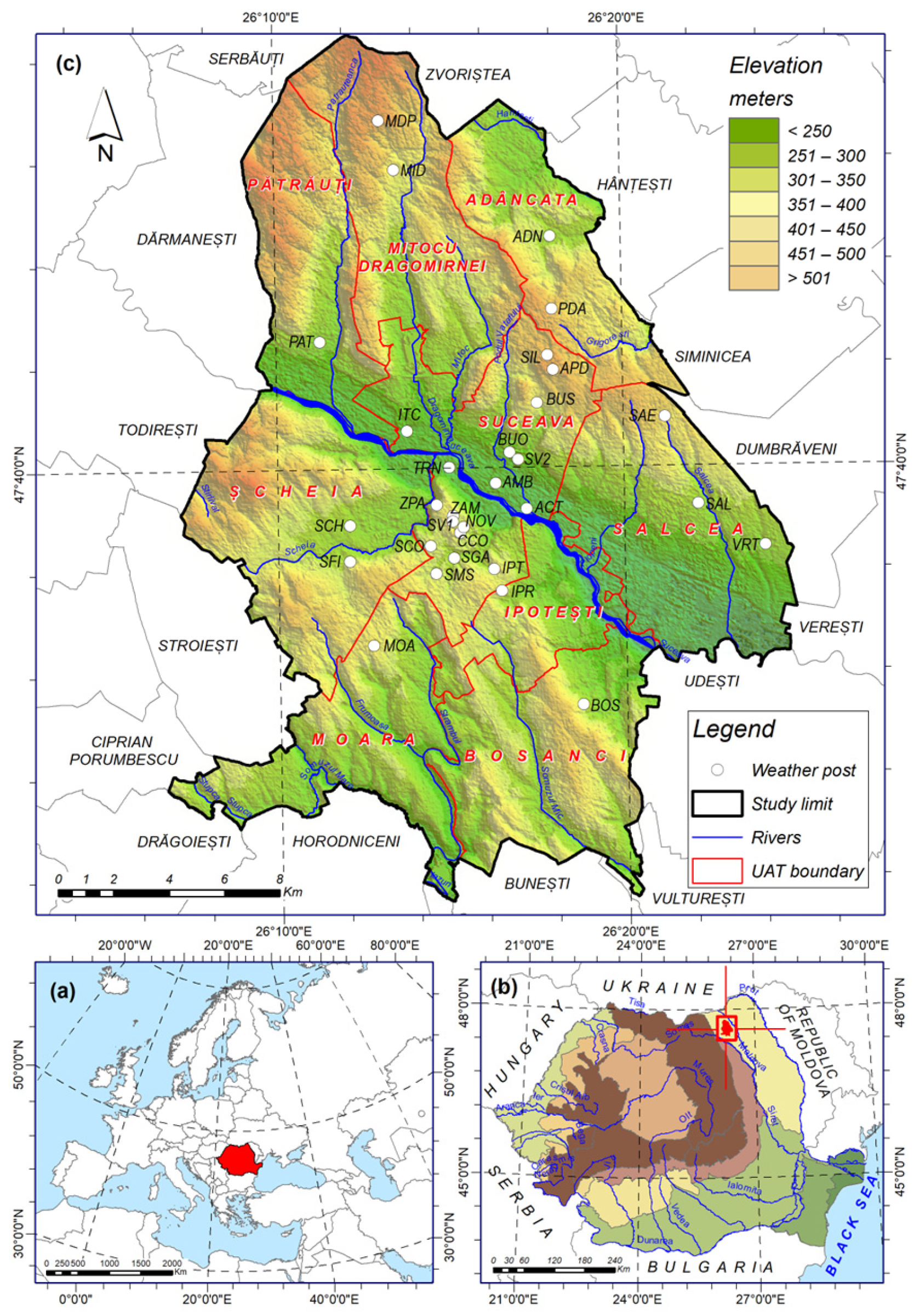
Figure 1. The location of SvMA in Europe (a), in the north-east of Romania (b), and the detailed physico-geographical conditions within the administrative boundaries [43], as well as the position of the meteorological posts and stations where the Tair2m observations were carried out during the 2019–2021 interval (c).
Remotesensing 16 02967 g001
Figure 2. The regression lines and equations for the measured and estimated values at the 31 observation points resulting from data interpolation through the method of multiple regression with IDW.
Remotesensing 16 02967 g002
Figure 3. The LCZs map of the Suceava metropolitan area (a). The share of different areas of the LCZs from SvMA surface (2023). (b) Designation of LCZ types in the metropolitan area of Suceava (c).
Remotesensing 16 02967 g003
Figure 4. Spatial distribution of the mean thermal values in SvMA in the interval 2019–2021 from in situ measurements at Tair2m (a) and Landsat LST (b) for the 35 analyzed time steps.
Remotesensing 16 02967 g004
Figure 5. Thermal profiles of Tair2m and LST on the NE–SW (a) and NW–SE (b) directions over SvMA during sunny summer days (2019–2021).
Remotesensing 16 02967 g005
Figure 6. Spatial distribution of the mean thermal values in the municipality of Suceava in the interval 2019–2021 for summer sunny days from Tair2m measurements (a) and LST satellite imagery (b) for the 35 analyzed time steps.
Remotesensing 16 02967 g006
Figure 7. Spatial distribution of the differences between the numerical models of Tair2m and LST (Tair2m—LST) for the 35 analyzed time steps of summer sunny days over SvMA in the interval 2019–2021.
Remotesensing 16 02967 g007
Figure 8. Histograms showing the Tair2m and LST baseline thermal parameters for SvMA and their differences for the 35 hourly sequences of in situ determinations synchronous to the 35 Landsat satellite scenes used in the thermal modeling for the summer days in the interval 2019–2021.
Remotesensing 16 02967 g008
Figure 9. IMD ratio regionalized by the kernel density estimation method for urban agglomerations (a) and city areas (b).
Remotesensing 16 02967 g009
Figure 10. NW–SE (a) and NE–SW (b) profile IMD ratio, over SvMA.
Remotesensing 16 02967 g010
Figure 11. The average values of Tair2m and LST on IMD thresholds obtained from gridded points at 500 m grids (1626 values) for SvMA (2019–2021).
Remotesensing 16 02967 g011
Table 1. Specifications of Landsat data [48] over the SvMA study area (June–August interval from 2019, 2020, and 2021).
SatellitesSensorsBandsSpatial
Resolution
Temporal ResolutionPathsRowPass Time (GMT)No. of Data
Series
Landsat 7ETM+Band 660 *(30) m16 days183/1842708:05–08:5211
Landsat 8OLI&TIRBand 10100 **(30) m16 days183/1842709:02–09:0824
* ETM + Band 6 is acquired at 60 m resolution, but products are resampled to 30-m pixels.
** TIR + Band 10 is acquired at 100 m resolution, but products are resampled to 30-m pixels.
Table 2. The performance of the 5 interpolated methods expressed as modulus values of differences between measured and estimated temperatures for SvMA (2019–2021); Dif.–Difference, MT-measured temperature, MR + IDW-multiple regression adjusted by IDW, MR + OK-measured temperature adjusted by ordinary kriging, SR-simple regression, SR + IDW-simple regression adjusted by ordinary kriging, SR + OK-simple regression adjusted by ordinary kriging.
PostIndexALT.SLOPEASPECTMTMR + IDWDif.MR + OKDif.SRDif.SR + IDWDif.SR + OKDif.
X1X2X3ABA–BCA–CDA–DEA–EFA–F
NOV123634.69130.2429.530.61.129.10.429.40.131.62.129.10.4
IPT163585.94256.6128.428.20.229.20.729.41.029.20.829.20.7
SFI153564.74305.5428.428.20.229.20.829.41.128.20.229.20.8
ZAM93684.56115.0230.429.90.529.11.229.41.028.91.529.11.2
APD234558.50290.7728.229.41.229.10.929.10.929.41.229.10.9
VRT243129.32229.7629.028.00.929.80.829.60.630.01.129.80.8
Mean 0.7 0.8 0.8 1.1 0.8
Table 3. The Tair2m–LST difference between the urban, peri-urban, and rural areas of SvMA (values obtained from the histograms of the numerical models Tair2m and LST).
Surface AreaTAir2mLSTTAir2m—LST
MinAvgMaxMinAvgMaxMinAvgMax
Urban area (IMD > 80%)30.632.233.926.935.853.23.7−3.6−19.3
Peri-urban area (IMD 40–80%)29.331.032.725.232.644.74.1−1.6−12
Rural area (IMD < 40%)26.929.932.123.630.439.13.3−0.5−7
Table 4. The thermal differences between Tair2m and LST by IMD classes extracted from 500 m grids (1626 values) for SvMA (2019–2021).
IMDTAir2mLSTTAir2m—LST
%MinAvgMaxMinAvgMaxMinAvgMax
<10%26.929.632.024.229.938.02.7−0.3−6.0
10–2028.330.333.426.431.236.71.9−0.9−3.3
20–3029.230.531.427.331.735.41.9−1.2−4.0
30–4029.530.631.428.132.037.81.4−1.4−6.4
40–5029.630.731.626.631.835.43.0−1.1−3.8
50–6029.630.831.728.132.336.21.5−1.5−4.5
60–7030.130.931.726.531.735.23.6−0.8−3.5
70–8030.231.332.628.433.336.81.8−2.0−4.2
80–9030.731.732.630.935.745.0−0.2−4.0−12.4
90–10031.432.633.931.137.045.10.3−4.4−11.2
Remotesensing 16 02967 i001
Table 5. The minimum, average, and maximum values for each LCZ class extracted from the Tair2m and LST model.
LCZ ClassNumber of
Meteorological Posts
The Indicatives of the
Meteorological Posts
TAir2mLSTTAir2m—LST
MinAvgMaxMinAvgMaxMin *Avg *Max *
10-32.132.433.334.738.046.0−2.6−5.6−12.7
26SCO, NOV, SV1, ZAM, SV2, BUO29.232.033.927.035.947.22.2−3.9−13.3
33CCO, ACT, ITC29.531.333.926.133.748.53.4−2.4−14.6
50-31.531.631.732.332.833.5−0.8−1.2−1.8
611BOS, MOA, IPR, IPT, SFI, SGA, VRT, SAL, BUS, PAT, ADN27.230.433.825.331.747.81.9−1.3−14.0
71TRN29.731.733.728.435.747.81.3−4.0−14.1
81AMB29.632.233.926.336.553.23.3−4.3−19.3
91MID27.029.431.524.929.636.82.1−0.2−5.3
100-29.932.133.729.138.147.50.8−6.0−13.8
A5ZPA, ADP, SIL, PDA, MPD26.928.131.923.626.536.73.31.6−4.8
B0-26.929.131.724.428.635.32.50.5−3.6
C0-28.730.633.225.230.938.53.5−0.3−5.3
D3SMS, SCH, SAE27.230.433.924.931.444.72.3−1.0−10.8
E0-29.130.933.927.232.549.91.9−1.6−16.0
F0-28.930.831.825.731.334.43.2−0.5−2.6
G0-27.529.832.424.828.037.82.71.8−5.4
Thermal indices of synthesis for SvMA26.930.833.923.632.57553.23.3−1.8−19.3
* Values resulting from mathematical calculation.
Disclaimer/Publisher’s Note: The statements, opinions and data contained in all publications are solely those of the individual author(s) and contributor(s) and not of MDPI and/or the editor(s). MDPI and/or the editor(s) disclaim responsibility for any injury to people or property resulting from any ideas, methods, instructions or products referred to in the content.