Article

Assessment of Hygroscopic Behavior of Arctic Aerosol by Contemporary Lidar and Radiosonde Observations

1
Alfred-Wegener-Institute, Helmholtz Centre for Polar and Marine Research, Telegrafenberg A45, 14473 Potsdam, Germany
2
Institute of Physics and Astronomy, University of Potsdam, Karl-Liebknecht Str. 24/25, 14476 Potsdam, Germany
*
Author to whom correspondence should be addressed.
Remote Sens. 2024, 16(16), 3087; https://doi.org/10.3390/rs16163087
Submission received: 19 July 2024 / Revised: 16 August 2024 / Accepted: 18 August 2024 / Published: 21 August 2024

Abstract

:
This study presents the hygroscopic properties of aerosols from the Arctic free troposphere by means of contemporary lidar and radiosonde observations only. It investigates the period from the Arctic Haze in spring towards the summer season in 2021. Therefore, a one-parameter growth curve model is applied to lidar data from the Koldewey Aerosol Raman Lidar (AWIPEV in Ny-Ålesund, Svalbard) and simultaneous radiosonde measurements. Hygroscopic growth depends on different factors like aerosol diameter and chemical composition. To detangle this dependency, three trends in hygroscopicity are additionally investigated by classifying the aerosol first by its dry color ratio, and then by its season and altitude. Generally, we found a complex altitude dependence with the least hygroscopic particles in the middle of the troposphere. The most hygroscopic aerosol is located in the upper free troposphere. A hypothesis based on prior lifting of the particles is given. The expected trend with aerosol diameter is not observed, which draws attention to the complex dependence of hygroscopic growth on geographical region and altitude, and to the development of backscatter with the aerosol size itself. In a seasonal overview, two different modes of stronger or weaker hygroscopic particles are additionally observed. Furthermore, two special days are discussed using the Mie theory. They show, on the one hand, the complexity of analyzing hygroscopic growth by means of lidar data, but on the other hand, they demonstrate that it is in fact measurable with this approach. For these two case studies, we calculated that the aerosol effective radius increased from 0.16 μ m (dry) to 0.18 μ m (wet) and from 0.28 μ m to 0.32 μ m for the second case.

1. Introduction

The Arctic, and especially the European sector in winter, shows a strong warming [1], a phenomenon which is called Arctic Amplification [2,3]. This Arctic Amplification is not fully understood due to a complex interplay between local and regional exchange processes [4]. Amongst others, variations in aerosols are found to lead to significant changes in the Arctic climate system [5]. Their direct effect [6] as well as the aerosol–cloud feedback [7] are complex and depend on the spatial and temporal distribution of the aerosols [8]. However, this feedback may play an important role in the Arctic Amplification.
Ny-Ålesund is located on the West coast of Spitsbergen in the European Arctic at (78.9N, 11.9E). It is an international super-site for environmental research, in which atmospheric measurements are carried out by many institutes from different European or Asian countries. Aerosol measurements were originally motivated by the Arctic Haze phenomenon, a springtime air pollution [9] transported into the Arctic from inhabited regions [10]. Other prominent aerosol types in this region are biomass burning [11], sulfates of different origin or sea salt [12].
These aerosol measurements have been performed both by in situ (e.g., [13]) and by remote sensing (e.g., [14]) methods for more than 20 years at that site. A current overview of the measurement efforts concerning in situ techniques is given in Platt et al. [15], and the trend and variability from a remote-sensing perspective are presented in Graßl and Ritter [16].
While a few studies have been published that combine both in situ and remote sensing information, like Ferrero et al. [17], this is generally a complicated task, because aerosol properties may change in the boundary layer on short time scales.
Arctic aerosols typically present a clear annual cycle as described by Tunved et al. [13]: there are slightly larger particles during the Arctic Haze period in spring, followed by a maximum aerosol concentration in summer of more and very small particles from a local origin (increased new particle formation [18]) and a clear autumn. Hence, from an aerosol perspective, a year may be subdivided into three periods: polluted in late winter and spring, local with sporadic biomass burning events in summer, and a clean season in autumn and early winter. As the aerosol’s radiative forcing not only depends on their intrinsic properties, but also on the albedo, solar altitude and background atmosphere [19], a precise estimation of this forcing is challenging.
Aerosols are difficult to describe in climate models for several reasons [20]. In this work, we investigate one of them in detail: the hygroscopic growth of these particles. Above a given relative humidity over water, an aerosol captures water molecules from the gas phase. Hence, it is growing in size and thus changes its light scattering properties [21,22,23]. We note that by the uptake and release of water molecules, not only the size but also the shape and the index of refraction of the scattering particles change. Hence potential differences between measured dry aerosol properties and the aerosol’s direct effect on the real atmosphere may partially be explained by hygroscopic effects.
The uptake or release of water from aerosols at changing relative humidity has been known for decades. Tang [21] considered the hygroscopic growth of different sulfate and nitrate aerosol particles and presented a hysteresis curve (his Figure 1): The aerosols remained at their dry radius at consecutively wetter conditions up to the deliquescence point. Beyond that, at even higher relative humidity, they take up water (they are “activated”) and may grow into a cloud droplet at about 100% relative humidity. At consecutively lower relative humidity, the aerosols are able to “defend” their water shell up to the efflorescence point. This means that aerosols that have been in contact with moist air before continuously change their diameter, and hence their scatter coefficient, depending on ambient humidity.
Frequently, this hygroscopic behavior of the scattering particles is described by a simple one-parameter power law of relative humidity with a hygroscopic exponent. Gassó et al. [22], for example, were able to separate different aerosol classes via that value, and Zieger et al. [24] presented an overview of aerosols’ hygroscopicity for several European sites. Vu et al. [23] also analyzed the hygroscopic behavior of an aerosol as a function of its dry diameter.
In Ny-Ålesund, the hygroscopic growth of Arctic aerosols was also analyzed by Zieger et al. [25], who performed measurements there during summer and fall using a dry and wet nephelometer. They found a surprisingly high hygroscopic behavior and a considerable sea salt fraction. Rastak et al. [26] extended similar measurements for a longer time period and concluded that during summer the aerosol was even more strongly hygroscopic than during spring time.
Lidar together with radiosonde data have been used to derive the hygroscopicity of aerosols so far in different regions of the world, like, e.g., in the U.S. (Dawson et al. [27]), or in China (Zhao et al. [28]). Wang et al. [29] even discussed the modification of the aerosol radiative forcing due to hygroscopic growth and found an increase in aerosol backscatter already below 40% relative humidity.
By this work we wanted to analyze to what extent the hygroscopic properties of aerosols can be derived by simultaneous observations from a multiwavelength lidar and a radiosonde for an Arctic site. We hypothesized that in the Arctic free troposphere (far away from the major sources of aerosols) vertical gradients of the aerosol properties, such as dry radius and chemical composition, should be low. Hence we posed the assumption that if changes in the aerosol properties occurred which coincided with gradients of the relative humidity, these changes would be due to hygroscopic effects, i.e., the uptake or release of water molecules from the aerosol particles. During their long advection from the source regions into the Arctic, an aerosol may frequently have encountered moist conditions and may have been activated. Therefore, remote regions like the Arctic may be well-suited locations to analyze hygroscopic effects of aerosol by lidar.
The paper is structured as follows: We shortly present our lidar and the radiosonde data in Section 2. Next the general situation on which this study is built is illustrated in Section 3. Using the lidar data, we present the development of the aerosol’s optical properties from spring to summer 2021, followed by an overview of the vertical trends in backscatter, color ratio and relative humidity over water. Further, an overview of their general hygroscopic properties is illustrated in Section 4. As this seasonal overview shows quite a bit of scatter, we discuss hygroscopicity in terms of its dependence on the aerosols’ size, season and altitude. Additionally, two case studies show the complexity of the different phenomena in some more detail. Finally, we try to put our findings in a more general perspective in Section 5. In particular, by using the Mie theory with properties obtained from lidar, we show that the hygroscopic growth of Arctic atmospheric aerosols is measurable and also above the boundary layer.

2. Instruments, Methods and Data

2.1. The Koldewey Aerosol Raman Lidar and Measurement Site

The data of this work were recorded by the Koldewey Aerosol Raman Lidar (KARL) at the AWIPEV station in Ny-Ålesund, Svalbard, ( 78 55.435 N 11 55.740 E), which is operated throughout the whole year. It is a traditional Raman lidar consisting of a Nd:YAG laser at 355 nm, 532 nm and 1064 nm. It collects both the elastically scattered light as well as the N 2 Raman lines at 387 nm and 607 nm by a 70 cm mirror and Licel electronics. It uses a Spectra-Newport laser operating at 10 W per color at 50 Hz. More information on the lidar can be found in Hoffmann [30].
This study used lidar data from April to the end of July 2021. The dataset consisted of a spatial resolution of 7.5 m and a temporal resolution of 10 min . As the investigation focused on tropospheric aerosol, only data up to 10.0 km are discussed.
In this work, we mainly considered the (volumetric) backscatter coefficient of an aerosol, β aer , in [ m 1 sr 1 ]. Another important quantity is the extinction coefficient α aer [ m 1 ]. Further, we defined the color ratio, the depolarization and the lidar ratio as:
CR ( λ 1 , λ 2 ) = β aer ( λ 1 ) β aer ( λ 2 ) δ aer ( λ ) = β aer ( λ ) β aer ( λ ) LR ( λ ) = α aer ( λ ) β aer ( λ )
However, as we dealt with daylight data, the noise in α aer limited the accessible altitude (see Appendix A.1). One needs to treat it with caution, which is why in this work, α aer and the lidar ratio LR were only analyzed up to a 2.5 km height.
For abbreviation purposes, if not stated otherwise, we considered the backscatter at 532 nm , written as β 532 , the color ratio CR ( 355 nm , 532 nm ) = β aer ( 355 nm ) β aer ( 532 nm ) , or in short CR 532 355 , and the depolarization and lidar ratio at 532 nm as well.
Information on the meteorologic conditions was obtained by a radiosonde: A Vaisala RS-41 was launched directly next to the lidar each day at around 11 UT . It provided radiosonde profiles of temperature, wind, humidity and pressure [31]. These sounding data were used to calculate the Rayleigh contribution of backscatter and extinction and more importantly for this work, to derive profiles of relative humidity.

2.2. Dataset and Cloud Mask

Lidar provides vertical profiles of optical aerosol properties from which one can obtain their microphysical properties. The standard methods of Ansmann [32] and Klett [33] were used to evaluate the lidar data. A boundary condition was needed for the retrieval of the backscatter. We chose the clear sky condition β total = 1.1 · β Rayleigh at 532 nm as the average in the altitude interval between 16 km and 18 km . Further, we used an Ångström exponent A = 1.2 to recalculate the corresponding boundary condition for the other wavelengths. For the Klett Method, the assumption of a lidar ratio was needed. We chose moderate lidar ratios of 36 sr for 355 nm and 42 sr for 532 nm according to [14,34].
Clouds cause high backscatter and thus destroy any statistics on aerosol properties. Therefore, lidar profiles with cloud influence need to be filtered out prior to performing any statistics on the aerosol. The first step is to apply a threshold-based cloud filter which removes affected time or altitude steps. Analyzing our data (scatter plot of color ratio versus aerosol backscatter at 532 nm ), we noted that a situation where β aer > 3 · β Rayleigh implied a cloud occurrence, and we removed these data points accordingly. Further, below clouds, the backscatter profile in a lidar might be off due to an inappropriately chosen lidar ratio within the cloud. For thin clouds, our retrieval software automatically corrected this as in Nakoudi et al. [35]. For thicker clouds, the lidar profiles either had to be rejected or recalculated using the assumption that in at least one altitude layer below the cloud, the aerosol backscatter remains constant.
After application of the cloud filter, out of 1046 lidar profiles, 451 remained. During the discussion of hygroscopic growth, simultaneous radiosonde (Vaisala RS-41) data were used. Then, only lidar data obtained ± 30 min before and after the launch of the radiosonde were considered, leading to 33 profiles over 10 days.
As previously mentioned, the study focused on tropospheric aerosols up to a 10.0 km height. In addition, due to the necessary overlap of telescope and laser beam from the lidar, only heights above 0.7 km were analyzed.

2.3. Hygroscopic Growth and the Growth Curve Model

The hygroscopicity of an aerosol describes its ability to grow due to water uptake. Next to the relative humidity of the atmosphere, it depends on both the aerosol’s size and chemical composition [24,36].
Tang [21] studied a salt-containing aerosol and found the hygroscopic growth to describe a hysteresis: for the activated aerosol, meaning aerosols that already grew at some earlier point in time, the hygroscopic growth started at 40 % relative humidity, while for the non-activated aerosol, it started at 80 % .
Hygroscopic growth changes the aerosol’s scattering and absorption properties [25,37]. Zieger et al. [25] and Gassó et al. [22] described this change by means of the hygroscopic growth curve model. It utilizes the scattering enhancement factor  f ( RH , λ ) , which they parametrized as:
f ( RH ) = ( 1 RH ) γ
with the relative humidity RH and the fit parameter  γ , which acts as a measure for the hygroscopicity of the aerosol.
Two comments about this Formula (2) are necessary: First, f usually refers to the scattering enhancement. A lidar measures primarily the backscatter, and we applied the same approach to our data. Hence, the γ values of our work are not directly comparable to the cited literature. Second, via water uptake, typically, the refractive index of the aerosol changes. For a few case studies with good lidar data quality, this effect can be deduced (e.g., Dube et al. [38]). However, as in the literature above, here, we neglected this and assumed that the index of refraction did not change with humidity. In addition, we performed simulations that demonstrated that the derivation of the dry and wet diameter did not critically depend on the refractive index. In addition, by keeping the size distribution as a constant, the backscatter was only proportional to the total number N of aerosols behind the distribution. We assumed that N stayed constant and a change in backscatter at a contemporary gradient in relative humidity was solely due to hygroscopic growth. The application of the growth curve was then feasible without precise knowledge of the aerosol concentration by using the normalized backscatter. It was normalized by dry conditions where hygroscopic growth cannot occur. Dry conditions are generally considered between 0% and 40% relative humidity but are adapted depending on the quality of the normalization.
However, note that an assumption about the unchangeable composition of the particles only holds locally, that is, for each day and each layer where we see a pronounced gradient in the relative humidity. The averaged chemical composition in the seasonal overviews acts as an indication of the average hygroscopic growth in the free troposphere and might thus help in the future to refine the lifetime of the different aerosol species.

3. Aerosol Properties in Spring and Summer 2021

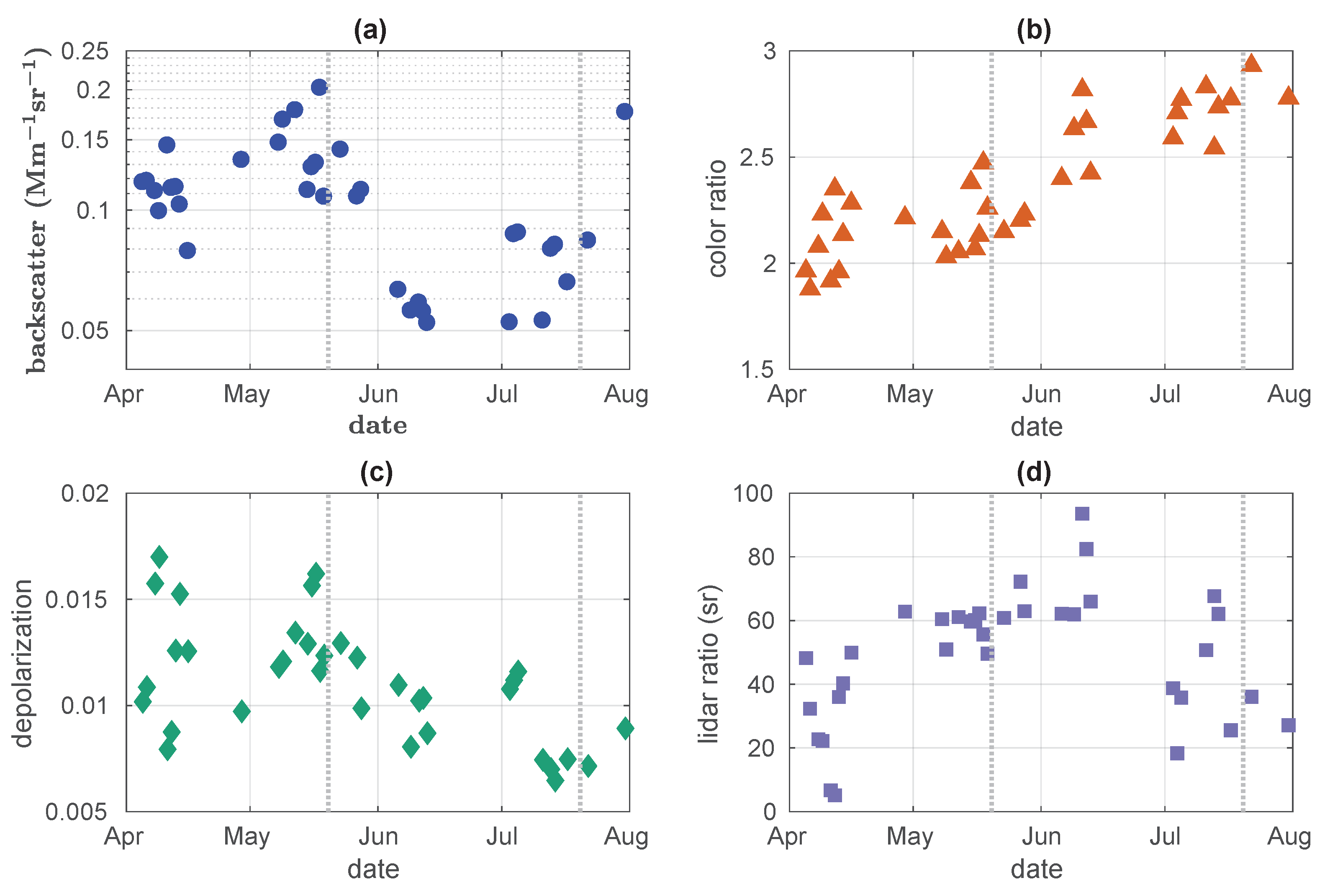
3.1. The Seasonal Aerosol Cycle from Spring to Summer 2021

The daily median of the aerosol backscatter, color ratio and depolarization between 0.7 km and 10.0 km and of the lidar ratio between 0.7 km and 2.5 km are illustrated in Figure 1a–d.
The backscatter development in Figure 1a exhibits an increase till mid-May, followed by a decrease till mid-June. Towards mid-July, the backscatter increases again. Considering the points of inflections on 20 May and 20 July, the period can be subdivided into three different seasons, as indicated by the vertical dotted lines in Figure 1a–d.
The color ratio in Figure 1b shows a continuous decrease in effective particle radius throughout the whole period.
The aerosol depolarization stays continuously low (see Figure 1c).
The lidar ratio is on average the highest in May and early June. In particular, 11 and 12 April have low values. It is noteworthy that the lidar ratio most often has values between 35 sr and 40 sr during the season, except for May and June. It is constantly enhanced and even provides two peaks in the lidar ratio on two consecutive days.

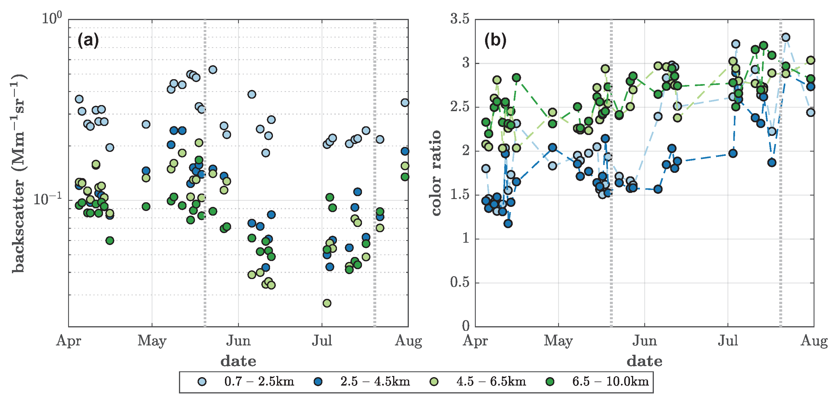
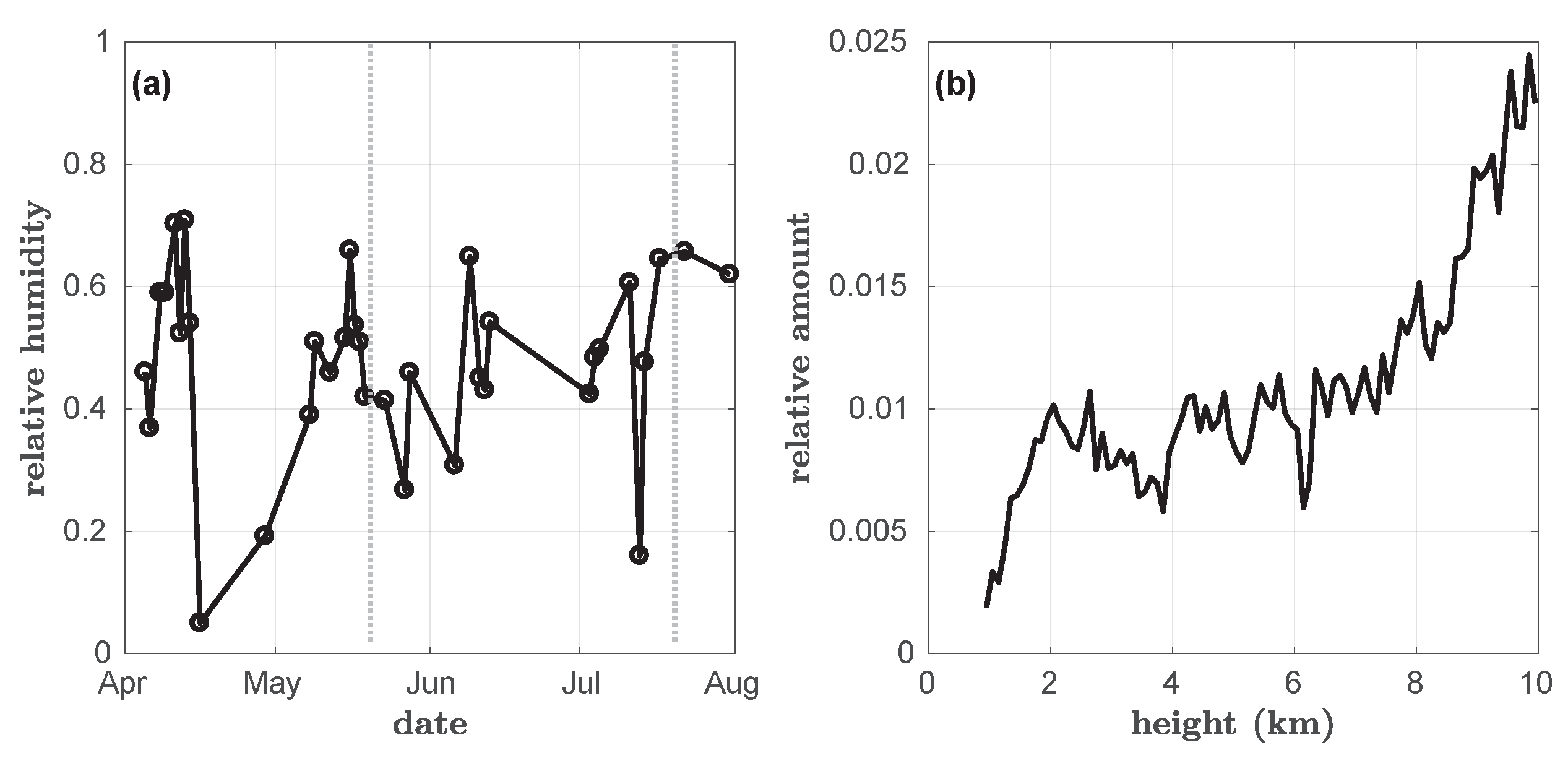
3.2. Vertical Trends in Backscatter and Color Ratio, and the Relative Humidity over Water of the Season

Figure 2a demonstrates the height dependence of the backscatter development. The daily median of the backscatter was built upon four different height intervals: 0.7–2.5 km , 2.5–4.5 km , 4.5–6.5 km and 6.5–10.0 km . Overall, the backscatter was most increased in the lowest height interval. However, the backscatter gradients in time were most pronounced at heights of 2.5 km to 6.5 km .
Figure 2b was built similarly to Figure 2a but illustrates the color ratio. In general, the color ratio increased towards the summer season for every height interval. Thereby, the lowest height interval (0.7–2.5 km ) provided the strongest gradient in time. The beginning of that increase was approximately after the spring season, which was estimated by means of the backscatter. Furthermore, the color ratio values were about 1.5 to 2.0 in the beginning and later rose to more than 2.5.
For a further evaluation of the impact of relative humidity on the seasonal trend (see Section 4.2), the average trend of relative humidity from April to July is shown in Figure 3a. From mid-April to May the values were comparably low. The forest fire-impacted season had on average the highest relative humidity of about 75 % . However, otherwise, no strong bias towards high or low relative humidity during a season was observed.
Although the absolute humidity decreased with altitude, the impact on the relative humidity was not clear, as the temperature decreased with altitude. The average, vertical distribution of relative humidity over water RH is illustrated in Figure 4a. Radiosonde points from the whole season, without limitation to temporal closeness to lidar data, were used. Data of low relative humidity (RH < 40 % ) can be treated all together, as hygroscopic growth occurs only for RH > 40 % ; thus, this is thus illustrated individually in Figure 3b.
It is visible that the relative humidity decreased with altitude. In particular, above 7 km , the amount of RH < 40 % increased strongly. Noteworthy is also the accumulation of relative humidity data points between 40% and 60% from 2 km to 4 km .
Figure 4b illustrates the relative amount of aerosol of specified color ratio within a certain height interval. A shift to higher color ratio values was observed above 5.0 km . The biggest aerosol gathered around 2.5–3.5 km , which correlated with the accumulation of relative humidity values between 40% and 60%. Note, also that the spread increased in this height interval so that aerosol with CR < 1 was especially allocated there. Above 7 km , the average color ratio began to reduce again, yet it was still bigger than the average values below 4.5 km . Above 9 km , the pattern became a more even distribution and in addition, a second concentration emerged which included very small aerosols ( CR > 4 ). Overall, there existed a clear trend of smaller aerosols at higher altitudes, yet not continuously decreasing.

4. Hygroscopic Properties

In this section, we present an overview of the general hygroscopic properties of Arctic aerosols for the whole season. Note that the relative humidity over ice, and thus ice nucleation, was not additionally considered. A further explanation for neglecting this effect is stated in Appendix A.2.
Figure 5a shows the backscatter development with regard to the relative humidity over water from April to the end of July 2021. Due to the high spread of 7.8 · 10 2 Mm 1 sr 1 in the backscatter, the median for each percentage of relative humidity is additionally illustrated. In general, the backscatter rose with the relative humidity. However, beginning at a relative humidity of 67 % , the behavior became more irregular and provided increased backscatter values.
For further analysis, in Figure 5b, a normalization of the median backscatter relative to dry conditions was performed. The drop in backscatter below 20 % relative humidity was considered as not representative for the expected constant course in dry conditions. Thus, “dry conditions” were taken here as the average backscatter coefficient between 20 % and 40 % relative humidity. The quality of the normalization was considered to be sufficient, as the constant course below 40 % was located around 1.0. The growth curve in Equation (2) was fitted to the normalized median backscatter between 41 % and 67 % relative humidity. By means of the assumption that disruptive effects would cancel out, due to the variety of meteorological events and aerosol size and composition, the fitting parameter γ could be considered as a seasonal average. It can be seen from the plot that already at 40 % relative humidity, the backscatter was larger than in dry conditions and that at 60 % , the backscatter was about 1.3 times larger than in the dry state.
Note that R2 amounted to only 0.43. To reduce the spread in backscatter and thus obtain a more precise fitting parameter γ , three subdivisions of the dataset were performed and are evaluated in the following Section 4.1, Section 4.2 and Section 4.3. The goal was to evaluate diameter-dependent, seasonal and vertical trends in hygroscopic growth of aerosols. The subdatasets in the following subsections are illustrated without an upper boundary in relative humidity. A robust least-squares fit was used for the application of the growth curve due to its stability against outliers.

4.1. Hygroscopic Growth Analysis, Dependent on Aerosol Diameter

A subdivision of the backscatter and radiosonde data from Figure 5 was performed. It was classified by the profiles’ median dry color ratios CR dry ( 355 nm , 532 nm ) and CR dry ( 532 nm , 1064 nm ) : Figure A3a in Appendix A.3 shows aerosols with CR dry ( 355 nm , 532 nm ) < 2 and 2 < CR dry ( 532 nm , 1064 nm ) < 3. Aerosols in Figure A3b fulfilled the conditions CR dry ( 355 nm , 532 nm ) 3.0 or CR dry ( 532 nm , 1064 nm ) 1.2 . The last subplot, Figure A3c, presents aerosols with 2 CR dry ( 355 nm , 532 nm ) < 3 and 1.2 < CR dry ( 532 nm , 1064 nm ) 1.7 . The choice of these color ratio intervals is explained later in Section 5.3. For now, just note that the subfigures are sorted in ascending order of aerosol diameter. As indicated by the median backscatter, the general development was a rise in backscatter with humidity, i.e., the occurrence of hygroscopic growth was still visible. Another observation is that the subdivision of the dataset mostly reduced the standard deviation σ . In particular, on the log-scale, a thinning of the spread in the data was visible compared to Figure 5a.
The hygroscopic growth curve was fitted to these subdatasets in Figure 6a–c. To improve the normalization in Figure 6a, reasonable dry conditions were considered to be between 30% and 40%. The fitting parameter γ was maximal for Figure 6b. Moreover, it indicated a particularly low hygroscopicity for Figure 6a.

4.2. Hygroscopic Growth Analysis, Dependent on the Season

The lidar and radiosonde data of Figure 5a were subdivided into whether they were recorded during Arctic Haze, the summer or the season with forest fire impacts. The classification of those seasons was based on Section 3.
The subdivided data are shown in Figure A4a–c in Appendix A.3. In general, backscatter still increased with relative humidity. Compared to the full dataset in Figure 5a, the spread in backscatter did not decrease significantly (see Figure A4a,b). Furthermore, because the complete daily trends were included in one subdataset, individual days that differed strongly from other days could have quite an impact on the overall trend. This was particularly visible in the smallest dataset—the forest fire-impacted season (see Figure A4c).
The growth curve was fitted onto the subdatasets (see Figure 7a–c). Two different modes were striking during the Haze and the summer season: one of lower and one of higher hygroscopicity. A weighting of the data points confirmed the fitting curves followed the different modes and estimated the aerosols’ hygroscopicity.
The modes of high hygroscopicity were almost identical for both seasons. However, the mode of low hygroscopicity during summer was stronger than during both Haze and forest fire-impacted season, as indicated by the fit parameter γ .

4.3. Hygroscopic Growth Analysis, Dependent on Altitude

The last hygroscopic growth analysis was performed on a dataset that was subdivided into altitude intervals. This subdivision is interesting as the aerosol size, chemical composition and relative humidity change with altitude. In accordance with Section 3, the following height intervals were used: 0.7–2.5 km , 2.5–4.5 km , 4.5–6.5 km and 6.5–10.0 km . Figure A5a–d illustrate the backscatter of the subdivided dataset, as well as its median. The standard deviation, in comparison with the analysis of the whole season (see Figure 5), was only partly reduced, as the average backscatter value of subplot Figure A5a,b was relatively high. Looking at the median backscatter, it seemed to be almost constant and merely fluctuating around a value.
The application of the growth curve (see Figure 8a–d) confirmed that observation, as the fit parameter γ at 2.5–4.5 km and 4.5–6.5 km was unreasonably low. Aerosols below 2.5 km provided a weak hygroscopicity (see Figure 8a). Above 6.5 km , there existed a comparably strong growth behavior (see Figure 8d).

4.4. Case Study: 23 May 2021

This case study addresses the visibility of hygroscopic growth within the variables color ratio, lidar ratio and aerosol depolarization in detail. In particular, we found distinct particle properties below 20 % relative humidity. Even if at this dry condition, no hygroscopic behavior can be expected, we present the results here and simply state that apparently, below this limit, the aerosol microphysics is different.
23 May 2021 was characterized by a strong gradient in relative humidity between 2.28 km and 3.28 km . Figure 9 shows the development of the color ratio (a) as well as the lidar ratio and aerosol depolarization (b) with relative humidity over water.
The color ratio CR 532 355 decreased from about 2.8 to 2.4. The color ratio CR 1064 532 , constructed from the longer wavelengths, was lower and rose from about 1.2 to 1.9. The aerosol depolarization was generally low and further decreased with increasing relative humidity. Apparently, the hygroscopic growth made the particles even more spherical, as one could imagine for a shell of water forming around the aerosol. Only at very dry conditions, the aerosol depolarization increased above 3 % . However, the dependence of the lidar ratio on relative humidity was not simple. We recall that the lidar ratio depends on all three parameters that determine the light scattering: the size, shape and refractive index [39]. All these variables change by the uptake or release of water molecules from the aerosol. As it can be seen from Figure 9, for 355 nm , the lidar ratio was low and more or less constant with low values below 20 sr , in particular above 20 % relative humidity. For 532 nm , the lidar ratio was more complicated: it peaked with values around 65 sr at about 30 % relative humidity.

4.5. Case Study: 29 April 2021

In this section, we discuss a second case study, this time for 29 April. By using this day, we wanted to demonstrate some caveats and difficulties which must be kept in mind when a combined evaluation between lidar and radiosonde for hygroscopic growth of aerosol is conducted.
We neglected the trivial case where the radiosonde and lidar may not probe the same air mass, because the radiosonde drifts with the wind and hence cannot see the advection of “new air masses”. One can overcome this by making sure that only cases are discussed that show a persistent structure in the lidar.
In Figure 10, an overview of this day in terms of relative humidity and aerosol backscatter is presented. While the lowest interval (1550 m to 1900 m) may point to a hygroscopic growth, the higher intervals (Figure 10b,c) clearly show a different behavior: while in the layer at altitudes between 3000 m and 3800 m, the relative humidity rose from slightly over 20 % to over 60 % , absolutely no increase in backscatter can be seen. There are two possible explanations for this finding: either the aerosol in this case is really non-hygroscopic and may, e.g., consist of soot, or (more likely) it consists of a normal hygroscopic aerosol that has not been activated before and was always trapped in dry air masses. In this case, the particles are always below their deliquescence point (as in Figure 1 of Tang [21]). While such cases may be rare in the Arctic (a long advection time of aerosols and cooling of the air masses, which enhances the relative humidity), they should be more frequent in the free troposphere above the inhabited continents.
Figure 10c shows the conditions in the altitude range between 6350 m and 6650 m , where a double layer in backscatter can be seen. In this case, the relative humidity is so low that no hygroscopic growth can be expected. This example simply shows that at least sometimes the aerosol is advected in dry air into the Arctic. In fact, Khattatov et al. [40] already noted that according to their observations, Arctic Haze either resulted from cold and dry source regions or underwent cloud formation processes.
The fact that no hygroscopic growth is visible in the layers around 3400 m or 6500 m can also be seen in Figure 11.
Figure 12 shows the lowest layer, at altitudes between 1550 m and 1900 m . While the relative humidity dropped significantly in this range, the color ratio CR 1064 532 rose. However, clearly, both quantities were not strictly correlated (see Figure 12a). This may indicate that (dry) particle properties were not precisely constant over this altitude interval. Neglecting this complication, Figure 12b shows the scatter plots of both color ratios as a function of relative humidity. It can be seen that the color ratio CR 532 355 remained almost constant at values around two.

5. Discussion

5.1. Estimation of the Effective Aerosol Radius—According to Mie Theory

In this section, we present an analysis of Mie calculations to quantify any change in the aerosol size by water uptake. Mie theory is a valid approximation as the aerosol depolarization, as presented in the previous sections, is generally small. It enables a deeper understanding of how the lidar variables change with particle diameter, and was already used by Ferrare et al. [41].
To represent an aerosol distribution, we chose a slim log-normal distribution with a geometric standard deviation of σ = 1.1 and a typical complex refractive index of Arctic aerosol of n = 1.5 + 0.01 i , as in Böckmann et al. [42]. This assumption of an index of refraction is a bit heuristic, as the precise value for both case studies and the change in the refractive index with humidity is not known. Contrarily, the choice of the geometric standard deviation is quite safe, as broader distributions cannot represent the measured changes in the color ratios and even more narrow distributions may be unlikely. We calculated for different effective radii of the aerosol the ratio of the backscatter efficiency coefficients at the three different wavelengths, i.e., the color ratios. The result is plotted in Figure 13.
Some interesting features can be seen from this plot. First, in both spectral regions, short wave and long wave, the color ratios do not decrease monotonically. This means that a plain statement like “the color ratios are an indicator of the particles’ size” is not strictly true. In fact, Figure 13 shows several intervals of aerosol radii, in which both color ratios show the opposite behavior. Second, the color ratio CR 532 355 contains the smaller information content, because for an aerosol effective radius between 0.2 μ m to 0.45 μ m , its value is always close to two.
For the case of 23 May, we observed an increase in CR 1064 532 from 1.2 (dry) to 1.9 (wet) (see Figure 9), while CR 532 355 decreased from values around 2.8 (dry) to 2.3 (moist). From the Mie calculations (see Figure 13), it can be seen that these values for the color ratios agreed with each other, and that the effective radius of the aerosol increased from about 0.16 μ m (dry) to 0.18 μ m (wet). These aerosol sizes are typical for the Arctic free troposphere based on lidar data [38]. This increase in the aerosol effective radius is highly relevant as can be seen from the increase in backscatter with humidity by a factor of three in Figure A6.
The second case from 29 April also showed values of the color ratios that were physically meaningful (see Figure 12b). In this example, the effective radius of the aerosol was around 0.32 μ m at around 1600 m at 80 % relative humidity, while it was approximately 0.28 μ m at around 1900 m at 50 % .
This non-monotonic behavior of the two color ratios from the Mie calculation also explains the complicated result of Figure 6, where the largest γ value was found for color ratios CR dry ( 355 nm , 532 nm ) 3.0 and CR dry ( 532 nm , 1064 nm ) 1.2 , which correspond to an effective radius of about 0.15 μ m (see Figure 13): both questions—how much does the aerosol radius increase with humidity and how apparent is this radius change in lidar data—need to be considered. Figure 14 shows the dependence of the aerosol backscatter at the three wavelengths of a Nd:YAG based lidar. The units in the figure are arbitrary, as they depend on the aerosol concentration that varies from case to case. Figure 14 uses the same log-normal distribution as before. It validates the previously mentioned observation of significant changes in backscatter for a seemingly small increase in aerosol size. Furthermore, it can be seen that larger particles have the highest backscatter. However, the gradient of how much the backscatter changes with the effective radius is not constant. The growth of aerosols with different dry radii is thus expressed differently in a backscatter-based growth curve as in Figure 6. In particular, for this situation, the backscatter gradient of 532 nm is the largest for an aerosol with a radius of about 0.15 μ m .
One obvious summary so far is that the information content from one color ratio alone is clearly limited (due to its non-monotonic behavior). However, with a three-wavelength system, the hygroscopic growth of aerosols in the accumulation mode can be tracked, because the backscatter changes for all wavelengths and both color ratios mostly show an opposite behavior. We note that for this discussion, the extinction values were not used, hence this methodology works in daylight, as in our case. Still, it would be beneficial to perform a real inversion (including the extinction coefficients) to retrieve the microphysical properties of aerosols, which would also allow us to estimate the change in the refractive index with humidity, as in Böckmann [43] and Dube et al. [38]. However, as our dataset also contained faint aerosol layers in the high troposphere during Polar day, the evaluation of the extinction coefficient was not always trustful; see Appendix A.1.

5.2. The Seasonal Cycle of Arctic Aerosol in 2021

Based on optical aerosol properties in Section 3, one can deduce the microphysical aerosol properties. The temporal development of these properties shows the seasonal cycle of the aerosol (see Figure 1a–d). In 2021, a return of the Haze period in May was observed. The lidar ratio was enhanced but not due to elongated particles [44] since the aerosol particles stayed spherical throughout the season (see Figure 1c). Instead, pollution was the reason, i.e., a return of the Arctic Haze. The Haze lasted approximately till 20 May, according to turning points in the backscatter developments. In comparison to May, April consisted of a clearer atmosphere—in particular on 11 and 12 April. Usually (e.g., [9,13]), the Haze maximum is observed in March or April. However, Shibata et al. [34] found the backscatter maximum from 2014 to 2017 to be on average in May, as in this study. However, they also found an increased aerosol load in June and July. This can be explained by inter-annual variability, as discussed in Graßl and Ritter [16]. In the last century, the Arctic Haze phenomenon also lasted until May (Herber et al. [45]). For this reason, it is important to continue monitoring the occurrence of aerosols in the Arctic.
After the Haze period, the typical summer season started (e.g., [13,46]). It was characterized by a small aerosol diameter (see Figure 1b) and lower backscatter (see Figure 1a), probably due to new particle formation [13].
Beginning on 20 July, the summer development was disturbed. As before, the lidar ratio and aerosol depolarization indicated the occurrence of pollution (see Figure 1c,d). Forest fire impacts were hypothesized as the reason for this disturbance.
The backscatter development within different height intervals is displayed in Figure 2a. It is visible that the aerosol number density was maximal in the lower troposphere. This was as expected (e.g., [47]), and in addition coincided during spring with the usual altitude range of the Arctic Haze [34,48]. In comparison, the transition from Arctic Haze to summer season, i.e., the seasonal cycle, was most pronounced between 2.5 km and 6.5 km . Shibata et al. [34] also stated that it was best to observe a seasonal cycle above 2 km . The weaker gradients, compared to the studies of Tunved et al. [13], stemmed from the integration of the lidar data over the altitude.
The color ratio development within the different height intervals (see Figure 2b) shows that in general, aerosols have a larger diameter in lower height intervals. This coincides with the studies of Rader et al. [49] and the location of the Haze [34,48]. A connection to hygroscopic growth is to be discussed later in Section 5.3. If we compare the color ratio of Figure 13 with typical sizes of Arctic aerosols as in Tunved et al. [13] or Dall’Osto et al. [50], which measured, even close to the ground, predominately aerosol radii smaller than 0.1 μ m , we notice that our sizes seem generally larger. Clearly, more regular and direct comparisons between aerosol in situ and remote sensing instruments are necessary. The existence of CR 532 355 values of about 1.5 only below an altitude of 2.5 km in March and April, which later increased to values around 2 and more, implies that only during the Haze period, at this low altitude, particles with an effective radius around 0.18 μ m prevail. Later in the year and always at higher altitudes, particles with effective radii around 0.15 μ m dominate.
Two obvious explanations why the aerosol diameter may be overestimated in lidar compared to in situ instruments can be immediately given: Figure 14 shows that the lidar signal is dominated by very few large particles which may not be captured efficiently by in situ techniques, or, simply, part of the aerosol is hygroscopically grown in the free Arctic atmosphere.

5.3. Dependence of Hygroscopicity on Particle Size, Season and Altitude

The hygroscopic analysis of all simultaneous lidar and radiosonde data from April to July 2021 (see Figure 5b) between 0.7 km and 10 km altitude provides a weaker growth than in the studies of Zieger et al. [25]. However, as described in Section 2.3 our values of the growth parameter γ were based on the backscatter coefficient and hence only roughly comparable to the existing literature. Further, we hypothesize that the sea salt fraction decreases with altitude: while sea salt may be one reason for the high hygroscopicity found by [26] and is frequent in the boundary layer of Ny-Ålesund as pointed out by [12], previous lidar studies suggest that sea salt is only a minor aerosol constituent above a 1 km altitude [14].
Overall, we noted a large spread in the overall hygroscopicity (see Figure 5). Therefore, subdivisions of the dataset were performed to reduce this spread. It was assumed that γ would then be determined more exactly. Moreover, another goal was the determination of hygroscopic trends dependent on aerosol diameter, season and altitude. Thus, this study provides information on hygroscopic properties of an average Arctic aerosol in this season. This is a major difference from previous studies, as they were mostly performed at either constant time or altitude (e.g., Navas-Guzmán et al. [51], Lv et al. [52]), except, e.g., Dawson et al. [27], who presented an overview of a campaign (based in the U.S.). Furthermore, our study includes the free troposphere, whereas studies have so far been often focused on the boundary layer (e.g., Lv et al. [52]).
  • Particle Diameter Trends
First of all, using Figure 13, the choice of the color ratio intervals in Section 4.1 leads to the following aerosol radii: Figure 6a corresponds to aerosols with a radius of about 0.11–0.12 μ m . Aerosols in Figure 6b have a radius of about 0.15 μ m , and the ones in Figure 6c have a radius of about 0.15–0.17 μ m . Hence, the hygroscopicity does not increase with the aerosol diameter in this analysis. However, this expected trend [23] is not doubted.
The results show that aerosol size is not the most important parameter in determining hygroscopic growth, unlike others, e.g., chemical composition. This critical dependence is also underlined by a case study from Lv et al. [52]. Thus, Figure 6 emphasizes the importance of the aerosols’ geographical location and altitude.
Furthermore, Figure 14 can be consulted to interpret the trend seen in hygroscopicity. The development of the backscatter coefficient of 532 nm with relative humidity shows the strongest gradient for a radius of around 0.15 μ m and is particularly low for smaller aerosols. It coincides with the observed high or low γ parameters in Figure 6a–c. Further research on the importance of the chemical composition compared to the aerosol size in terms of its hygroscopicity needs to be performed for a final evaluation of these two hypotheses. The unambiguous classification of even larger aerosols by their dry color ratio is desirable but not feasible here.
  • Seasonal Trends
In this work, we generally (Figure 7) found two modes with higher or lower values of the growth parameter. Only for the days in July with increased backscatter (biomass burning) was the mode of high γ missing (see Figure 7c). A low hygroscopicity for biomass burning was also found by [53,54].
We hypothesize that our finding with the mode of weak hygroscopicity can be explained by one of the following circumstances: T he particles have not been activated, as in the case of Section 4.5, which is indeed more likely for the drier upper free troposphere (Figure 3). Alternatively, the particles are already so large that any further growth cannot be captured well by the color ratio only in lidar data [42]. Finally, the aerosol in the upper free troposphere may simply be less hygroscopic; see next paragraph.
  • Vertical Trends
In this study, we analyzed to our knowledge for the first time the hygroscopic behavior of Arctic aerosols vertically resolved in the free troposphere. In our dataset from 2021, on average, no hygroscopic growth was visible from 2.5 km to 6.5 km (see Figure 8b,c). We explain this by the fact that with the increasing altitude, the surrounding air becomes drier (Figure 3) and the aerosol may become smaller. These two effects hinder the hygroscopicity. Further, Figure 8 shows the highest variability in the middle two altitude intervals.
From 0.7 km to 2.5 km , the aerosol is weakly hygroscopic (see Figure 8a). Due to the orography of Svalbard, one can hypothesize that underneath 2.5 km , interactions with the boundary layer still occur, meaning that, e.g., more moisture from the ocean or sea salt aerosol is present. Furthermore, assuming vertical wind shear, the spread in color ratio from 2.5–3.5 km (see Figure 4a) results from the mixing of different aerosols, if the free troposphere is in fact located above 2.5 km .
The most hygroscopic aerosol is present above 6.5 km (see Figure 8d). We explain this surprising result by the fact that the sources of the aerosol are close to the ground. Hence, an aerosol above 6.5 km has necessarily been rising with the surrounding air. Ascending air cools, which increases the relative humidity. Further, the aerosol in this air might be the oldest and during its aging, an Arctic aerosol changes from a chemically external to an internal mixture, meaning that less hygroscopic aerosol is surrounded by a shell of more hygroscopic sulfate [55]. Hence, we hypothesize that the fraction of aerosol in this altitude that has been in contact with moist conditions is higher than below 6.5 km . Therefore, the less hygroscopic, non-activated branch is missing in the upper troposphere. This finding is in agreement with [56] who stated that high Arctic black carbon (and aerosol) layers in the Arctic are controlled by cloud processes.
In total, we found a surprising complex vertical hygroscopicity, which needs to be analyzed further.

6. Conclusions

Herein, to our knowledge for the first time, hygroscopic properties of aerosols from the real, Arctic free troposphere were examined vertically by lidar. The study focused on tropospheric aerosols from the European Arctic from spring to summer 2021. Therefore, first, the seasonal development of the microphysical aerosol properties was investigated. The main results built the average situation of this season, on which the analysis of this study was based: an extended Arctic Haze till 20 May, followed by the typical summer season. Forest fire impacts were disruptive beginning on 20 July.
The main analysis, focusing on the aerosols’ hygroscopicity, included the following tasks in particular:
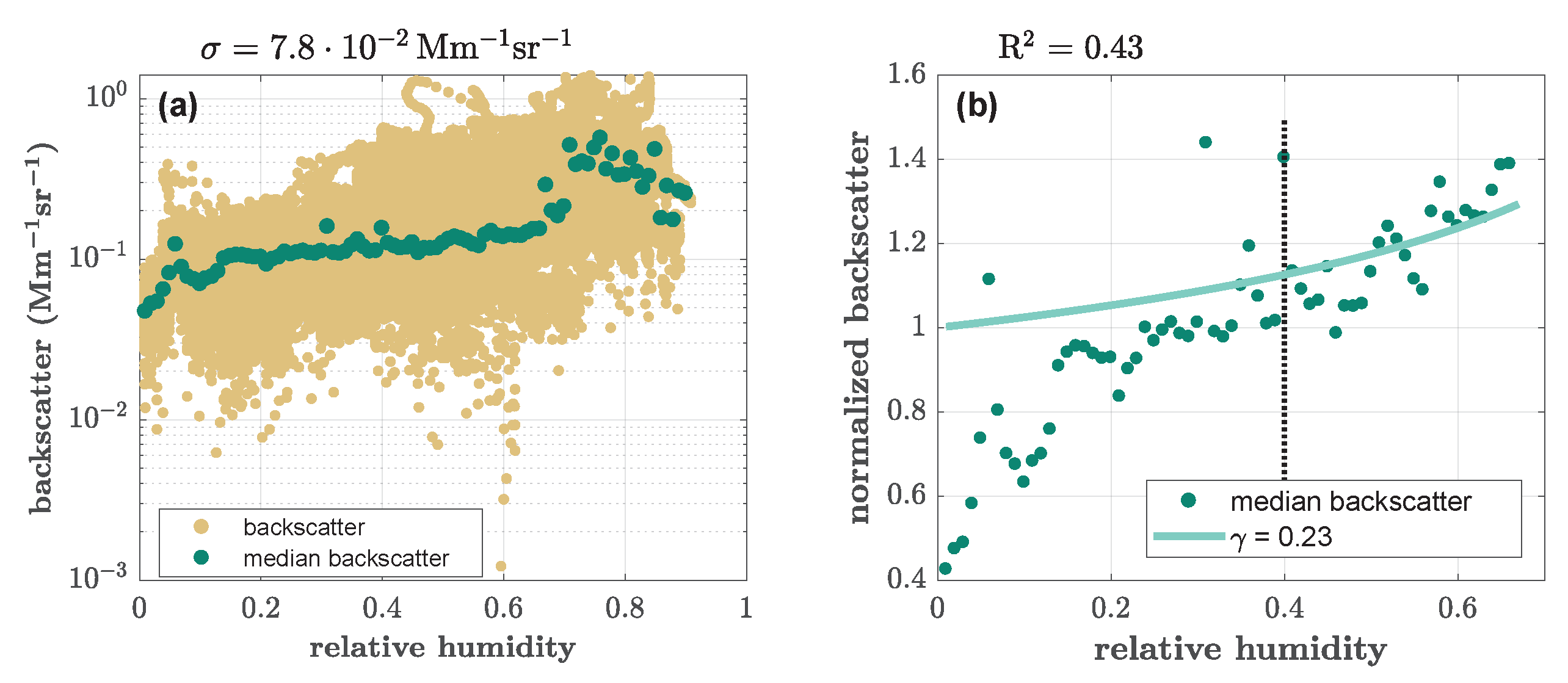
  • A subdivision of the dataset according to the aerosols’ color ratio, season and altitude. The application of the growth curve model then estimated the hygroscopicity of the subdataset.
  • An illustration of the often complex interpretation of the lidar data, and in particular, the color ratio. A Mie calculation was performed to obtain the relation between the color ratio and the effective aerosol radius. We showed that by three backscatter coefficients (two color ratios, no extinction coefficient) the hygroscopic growth for a large, relevant size interval could be captured with only mild assumptions on the refractive index.
Assessing these investigations led to the following results:
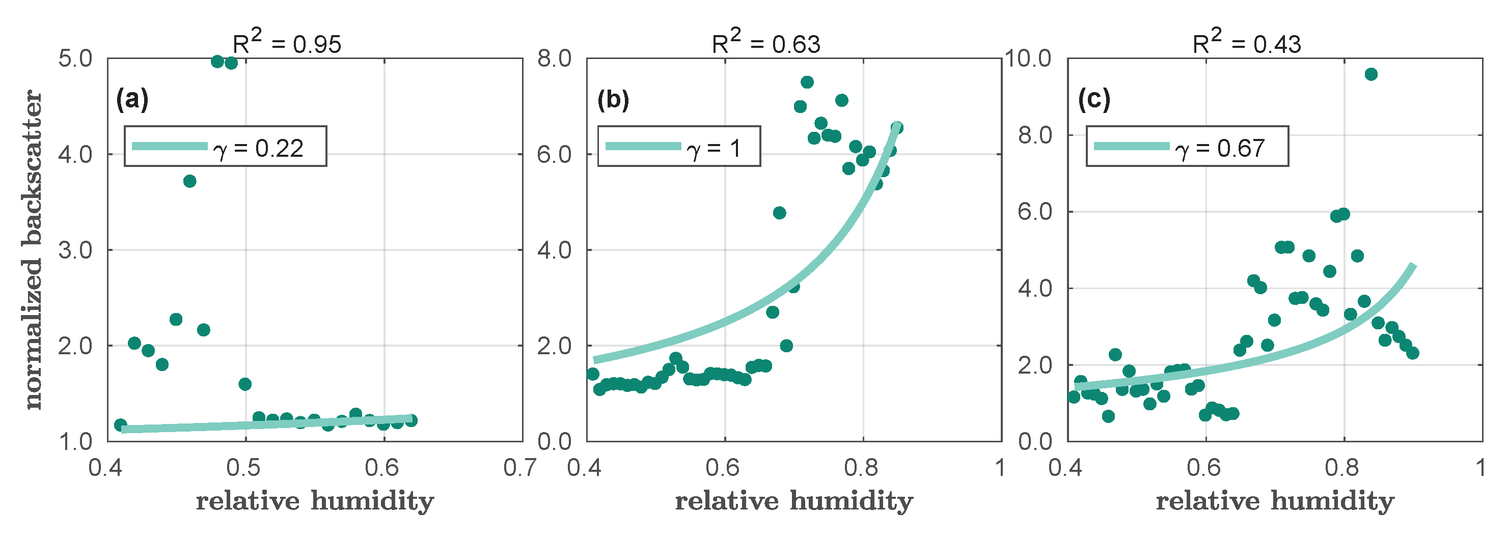
  • No clear trend in the hygroscopic growth with regard to the aerosol diameter could be observed. This probably resulted from its strong dependence on the aerosols’ geographical location and altitude, or even the development of backscatter with the particle radius itself (according to Mie theory). The hygroscopic growth of larger particles surely happens in the atmosphere, but it is hard to see from the inspection of the color ratio alone. Here, a full inversion of the lidar data seems necessary.
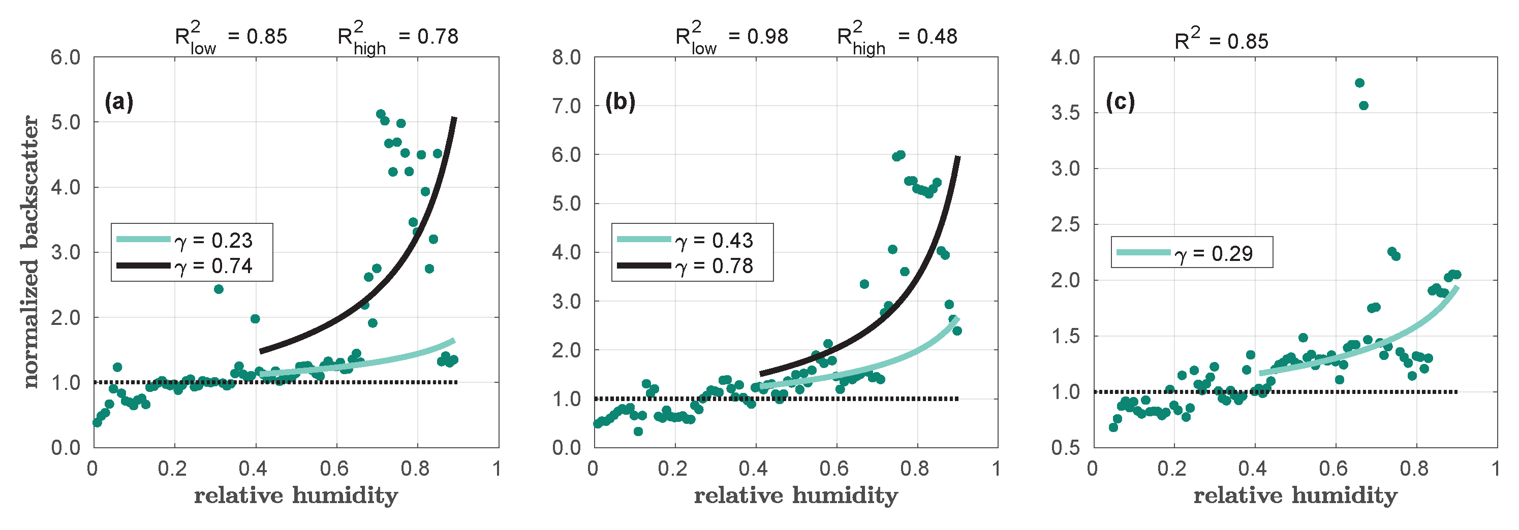
  • Generally, we found two modes in hygroscopicity in different seasons: one of stronger ( γ 0.75 , only missing during the forest fire season) and one of weaker ( γ 0.25 ) hygroscopicity. During summer only, this weakly hygroscopic mode had a higher γ value. Since this hygroscopicity parameter in the present work was based on the aerosol backscatter coefficient, this number may not be directly comparable to the existing literature. However, in the atmospheric column, the aerosol may, on average, be less hygroscopic than previously derived by ground-based measurements.
  • An interplay of processes causes the vertical trend in hygroscopicity to be complex. We found higher hygroscopicity and high relative humidity in the lowest altitude but could not say whether this was due to a different chemical composition or due to orographic effects. In the middle troposphere, the hygroscopicity was reduced, maybe because the probability of having aerosols that never encountered moist conditions is the highest. Finally, in the upper free troposphere, highly hygroscopic aerosols were found. These particles must have been lifted up, hence the surrounding air had apparently cooled to saturation level prior to its advection towards the Arctic. Case studies enabled this further detangling of the complex vertical trend.
In the future, a similar work could be performed during the Polar night to capture the full annual cycle and to systematically include the extinction coefficient from the Raman method. Coordinated observations by wind lidar in the lowest atmospheric layers may shed some light on vertical movements of air and their impact on humidity and hygroscopic growth.

Author Contributions

This study was jointly designed by N.E. and C.R. The evaluation of the lidar data and the writing of the manuscript was mainly performed by N.E. S.G. provided the Figures for the Mie calculations. C.R. is the PI of the lidar study and supervised N.E. and S.G. All authors have read and agreed to the published version of the manuscript.

Funding

This research received no external funding.

Data Availability Statement

The data presented in this study are available on request from the corresponding author.

Acknowledgments

The lidar measurements were performed by Sandra Graßl and Wilfried Ruhe. The authors thank the team of AWIPEV station for their support.

Conflicts of Interest

The authors declare no conflicts of interest.

Appendix A

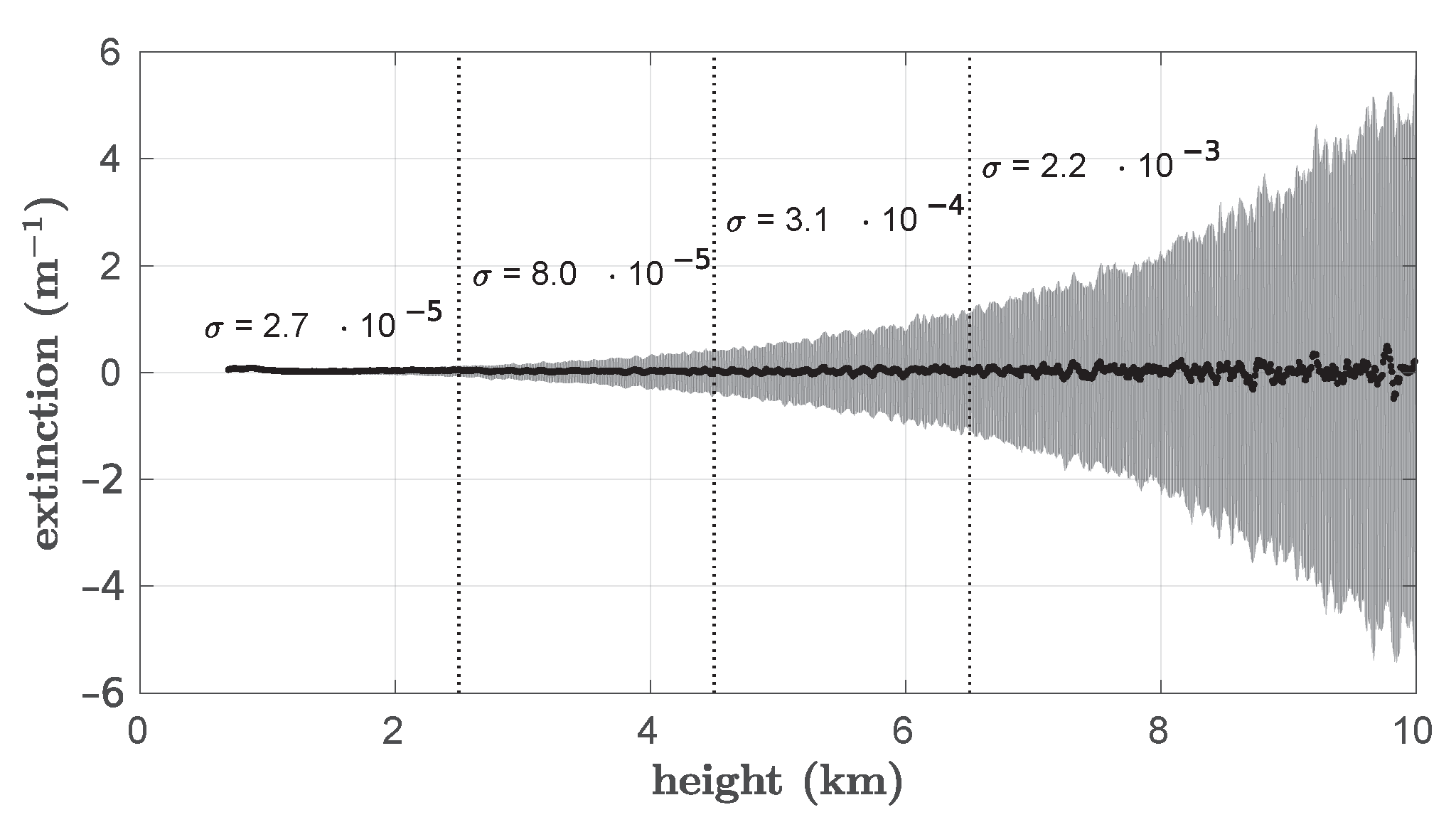
Appendix A.1. Sensitivity Study: Amplifying Noise in the Extinction Coefficient with Altitude

Figure A1. The median extinction over all available data points (without cloud influence) was calculated and is displayed for each height step. The standard deviation for each height step is illustrated as a filled area. It demonstrates the strongly increasing noise in extinction and thus the lidar ratio with altitude. For the previous analysis in this paper, the height intervals 0.7–2.5 km , 2.5–4.5 km , 4.5–6.5 km and 6.5–10.0 km were often utilized. In particular, the lidar ratio was only used within the lowest height interval due to noise. To emphasize this strengthening in noise, the mean standard deviation within this height interval is denoted in the figure. It rose by a magnitude of about 2.
Remotesensing 16 03087 g0a1

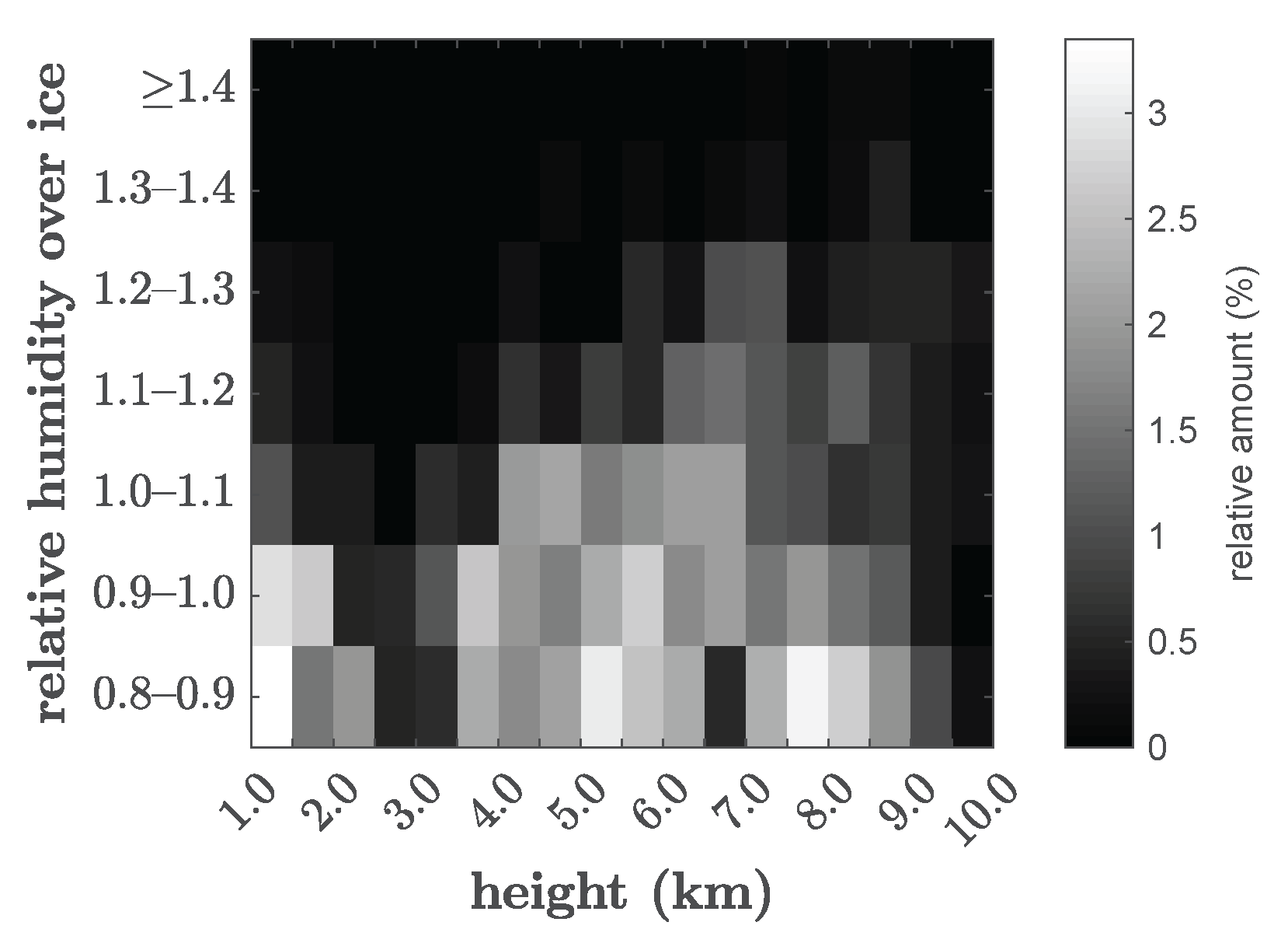
Appendix A.2. Discussion on the Importance of Relative Humidity over Ice in This Work

In this work, only the relative humidity over water was considered. This was due to the general sparseness of INP [57]: at a given supersaturation over ice, the onset of hygroscopic growth in the ice phase depends on the availability of INP, which may or may not be present. This potentially leads to a large scatter in the γ parameter.
Figure A2. The vertical distribution of the relative humidity over ice is shown. Significant supersaturation (>110%) occurs only above a 4 km altitude.
Remotesensing 16 03087 g0a2
Figure A2 presents the occurrence of supersaturation with respect to ice in our dataset. It can be seen that significant supersaturation (>110%) only occurred above a 4 km altitude. It was shown in Section 3 that at that altitude, the aerosol backscatter was already clearly lower than in the lower free troposphere.
However, principally contemporary measurements by radiosonde and depolarization lidar allow the creation of statistics, in which season, altitude, relative humidity and temperature ice or water clouds will form.

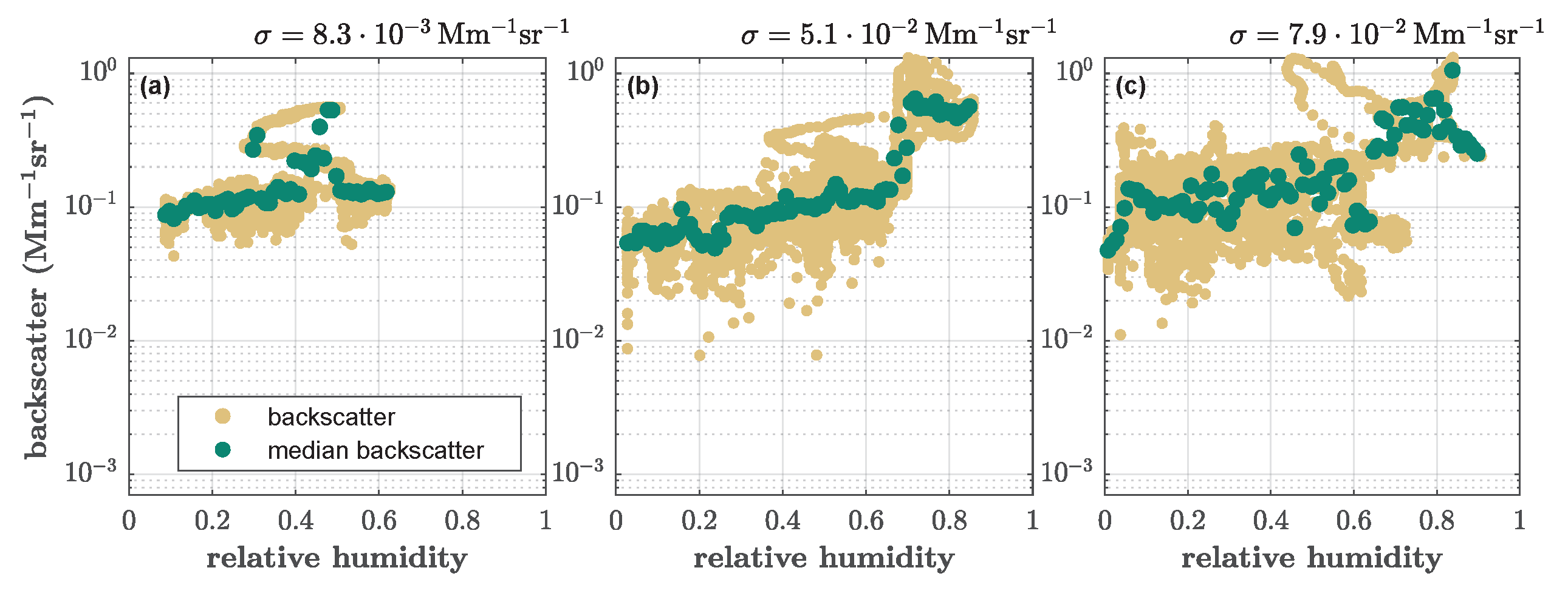
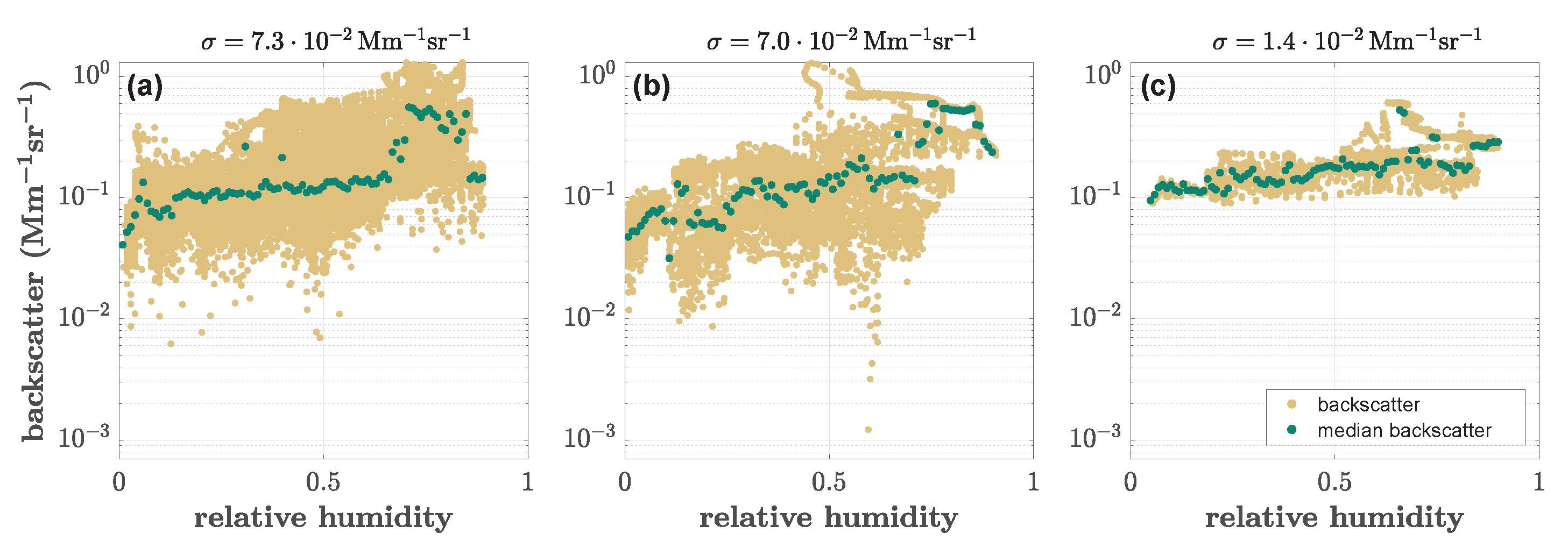
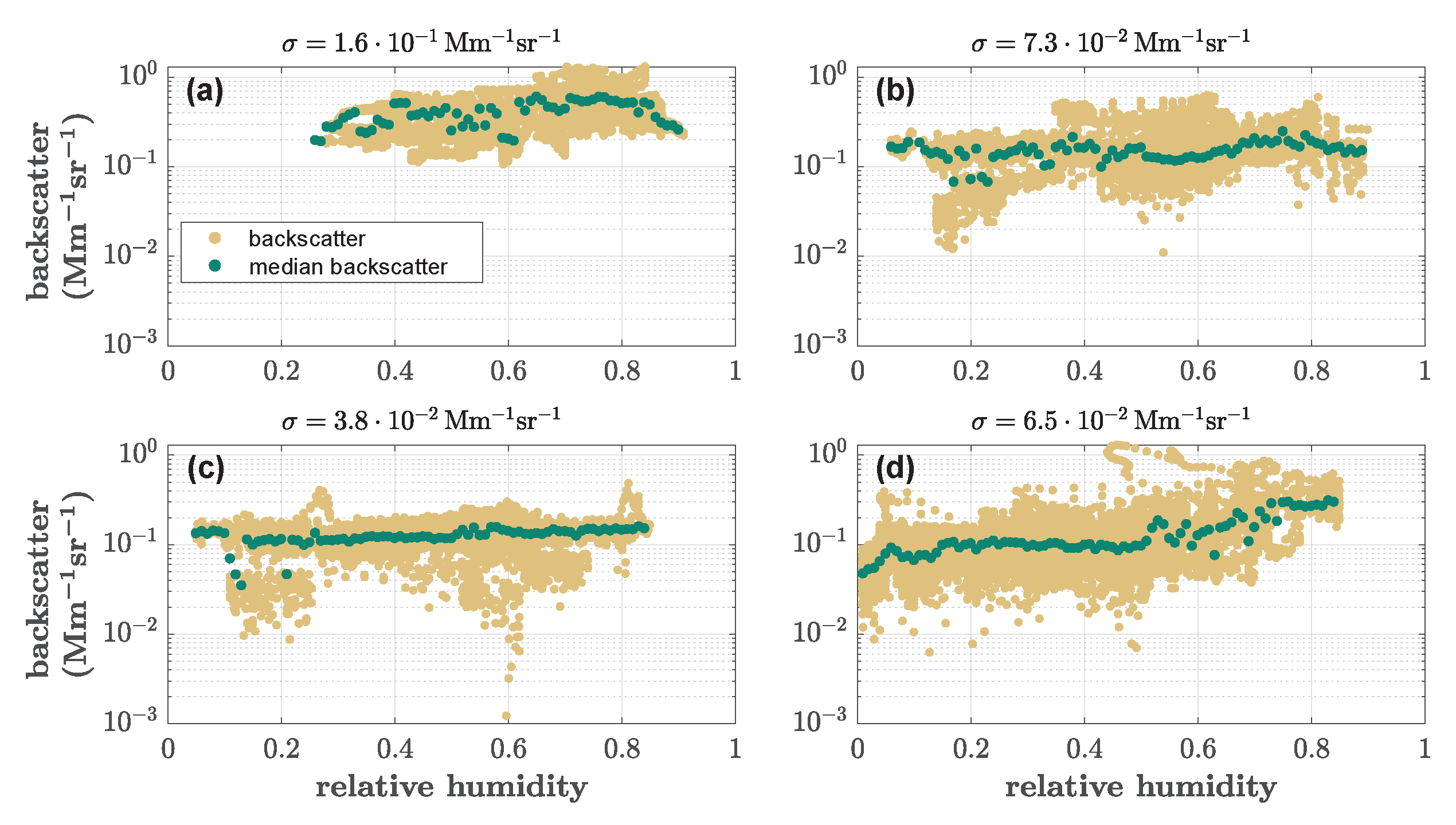
Appendix A.3. Backscatter Development with Relative Humidity for the Subdivided Datasets

The backscatter developments with regard to relative humidity for the subdivided datasets of Section 4.1, Section 4.2 and Section 4.3 are shown. The plots were built similar to Figure 5a, which displays the whole season. These overview plots are important to evaluate the quality of the subdivision by, e.g., a reduction in the spread of the backscatter. Moreover, outliers in the normalized median backscatter, used later for the growth curve, can be understood further.
Overall, the hygroscopic growth, meaning a rise in backscatter with humidity, as well as a reduction in the spread of the backscatter are mostly visible in all subdatasets.
Figure A3. The backscatter and radiosonde data from April to July 2021 were subdivided according to the profiles’ median dry color ratios. The intervals were the following: (a) CR dry ( 355 nm ,   532 nm ) < 2 and 2 < CR dry ( 532 nm ,   1064 nm ) < 3 , (b) CR dry ( 355 nm ,   532 nm ) 3.0 or CR dry ( 532 nm ,   1064 nm ) 1.2 , (c) 2 CR dry ( 355 nm ,   532 nm ) < 3 and 1.2 < CR dry ( 532 nm ,   1064 nm ) 1.7 . The median backscatter was calculated for each percentage of relative humidity. Overall, the backscatter still rises with humidity, as expected.
Remotesensing 16 03087 g0a3
Figure A4. The lidar and radiosonde data were subdivided into the three seasons, Arctic Haze (a), summer (b) and season with forest fire impacts (c). This separation was based on Section 3. To visualize an average growth behavior of the season, the median backscatter was calculated for each percentage of relative humidity. Note that backscatter developments of individual time steps may have a great impact on the overall trend.
Remotesensing 16 03087 g0a4
Figure A5. The dataset was subdivided by altitude. The backscatter and median backscatter between 0.7–2.5 km (a), 2.5–4.5 km (b), 4.5–6.5 km (c) and 6.5–10.0 km (d) are illustrated.
Remotesensing 16 03087 g0a5

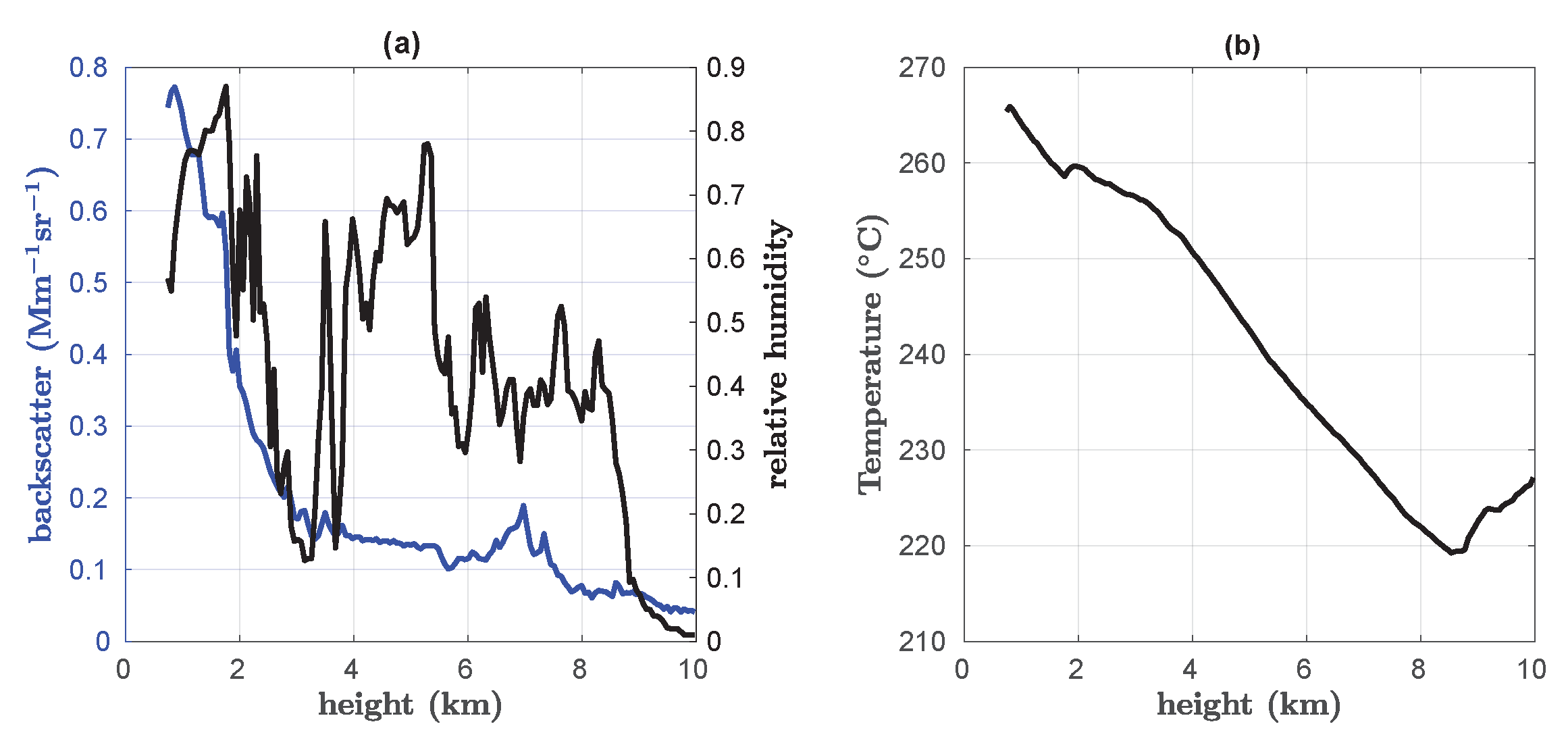
Appendix A.4. Backscatter, Relative Humidity and Temperature Profiles on 23 May 2021

Figure A6. The tropospheric profiles from backscatter, relative humidity (a) and temperature (b) are illustrated. A strong gradient in relative humidity is visible from 2.28 km to 3.28 km . A focused analysis of this interval was performed in Section 4.4.
Remotesensing 16 03087 g0a6

References

  1. Maturilli, M.; Herber, A.; König-Langlo, G. Surface radiation climatology for Ny-Ålesund, Svalbard (78.9 N), basic observations for trend detection. Theor. Appl. Climatol. 2015, 120, 331–339. [Google Scholar]
  2. Wendisch, M.; Brückner, M.; Crewell, S.; Ehrlich, A.; Notholt, J.; Lüpkes, C.; Macke, A.; Burrows, J.; Rinke, A.; Quaas, J.; et al. Atmospheric and surface processes, and feedback mechanisms determining Arctic amplification: A review of first results and prospects of the (AC) 3 project. Bull. Am. Meteorol. Soc. 2023, 104, E208–E242. [Google Scholar]
  3. Serreze, M.C.; Barry, R.G. Processes and impacts of Arctic amplification: A research synthesis. Glob. Planet. Chang. 2011, 77, 85–96. [Google Scholar] [CrossRef]
  4. Previdi, M.; Smith, K.L.; Polvani, L.M. Arctic amplification of climate change: A review of underlying mechanisms. Environ. Res. Lett. 2021, 16, 093003. [Google Scholar] [CrossRef]
  5. Stjern, C.W.; Lund, M.T.; Samset, B.H.; Myhre, G.; Forster, P.M.; Andrews, T.; Boucher, O.; Faluvegi, G.; Fläschner, D.; Iversen, T.; et al. Arctic Amplification Response to Individual Climate Drivers. J. Geophys. Res. Atmos. 2019, 124, 6698–6717. [Google Scholar] [CrossRef]
  6. Schmale, J.; Zieger, P. Aerosols in current and future Arctic climate. Nat. Clim. Chang. 2021, 11, 95–105. [Google Scholar] [CrossRef]
  7. Creamean, J.M.; Barry, K.; Hill, T.C.J.; Hume, C.; DeMott, P.J.; Shupe, M.D.; Dahlke, S.; Willmes, S.; Schmale, J.; Beck, I.; et al. Annual cycle observations of aerosols capable of ice formation in central Arctic clouds. Nat. Commun. 2022, 13, 3537. [Google Scholar] [CrossRef]
  8. Li, J.; Carlson, B.E.; Yung, Y.L.; Lv, D.; Hansen, J.; Penner, J.E.; Liao, H.; Ramaswamy, V.; Kahn, R.A.; Zhang, P.; et al. Scattering and absorbing aerosols in the climate system. Nat. Rev. Earth Environ. 2022, 3, 363–379. [Google Scholar] [CrossRef]
  9. Quinn, P.K.; Shaw, G.; Andrews, E.; Dutton, E.; Ruoho-Airola, T.; Gong, S. Arctic haze: Current trends and knowledge gaps. Tellus B Chem. Phys. Meteorol. 2007, 59, 99–114. [Google Scholar]
  10. Stohl, A. Characteristics of atmospheric transport into the Arctic troposphere. J. Geophys. Res. Atmos. 2006, 111. [Google Scholar] [CrossRef]
  11. Zielinski, T.; Bolzacchini, E.; Cataldi, M.; Ferrero, L.; Graßl, S.; Hansen, G.; Mateos, D.; Mazzola, M.; Neuber, R.; Pakszys, P.; et al. Study of chemical and optical properties of biomass burning aerosols during long-range transport events toward the arctic in summer 2017. Atmosphere 2020, 11, 84. [Google Scholar] [CrossRef]
  12. Udisti, R.; Bazzano, A.; Becagli, S.; Bolzacchini, E.; Caiazzo, L.; Cappelletti, D.; Ferrero, L.; Frosini, D.; Giardi, F.; Grotti, M.; et al. Sulfate source apportionment in the Ny-Ålesund (Svalbard Islands) Arctic aerosol. Rend. Lincei 2016, 27, 85–94. [Google Scholar]
  13. Tunved, P.; Ström, J.; Krejci, R. Arctic aerosol life cycle: Linking aerosol size distributions observed between 2000 and 2010 with air mass transport and precipitation at Zeppelin station, Ny-Ålesund, Svalbard. Atmos. Chem. Phys. 2013, 13, 3643–3660. [Google Scholar] [CrossRef]
  14. Ritter, C.; Neuber, R.; Schulz, A.; Markowicz, K.; Stachlewska, I.; Lisok, J.; Makuch, P.; Pakszys, P.; Markuszewski, P.; Rozwadowska, A.; et al. 2014 iAREA campaign on aerosol in Spitsbergen–Part 2: Optical properties from Raman-lidar and in-situ observations at Ny-Ålesund. Atmos. Environ. 2016, 141, 1–19. [Google Scholar]
  15. Platt, S.M.; Hov, Ø.; Berg, T.; Breivik, K.; Eckhardt, S.; Eleftheriadis, K.; Evangeliou, N.; Fiebig, M.; Fisher, R.; Hansen, G.; et al. Atmospheric composition in the European Arctic and 30 years of the Zeppelin Observatory, Ny-Ålesund. Atmos. Chem. Phys. Discuss. 2021, 22, 3321–3369. [Google Scholar]
  16. Graßl, S.; Ritter, C. Properties of arctic aerosol based on sun photometer long-term measurements in Ny-Ålesund, Svalbard. Remote Sens. 2019, 11, 1362. [Google Scholar] [CrossRef]
  17. Ferrero, L.; Ritter, C.; Cappelletti, D.; Moroni, B.; Močnik, G.; Mazzola, M.; Lupi, A.; Becagli, S.; Traversi, R.; Cataldi, M.; et al. Aerosol optical properties in the Arctic: The role of aerosol chemistry and dust composition in a closure experiment between Lidar and tethered balloon vertical profiles. Sci. Total. Environ. 2019, 686, 452–467. [Google Scholar] [PubMed]
  18. Schmale, J.; Baccarini, A. Progress in Unraveling Atmospheric New Particle Formation and Growth Across the Arctic. Geophys. Res. Lett. 2021, 48, e2021GL094198. [Google Scholar] [CrossRef]
  19. Nakoudi, K.; Ritter, C.; Böckmann, C.; Kunkel, D.; Eppers, O.; Rozanov, V.; Mei, L.; Pefanis, V.; Jäkel, E.; Herber, A.; et al. Does the Intra-Arctic Modification of Long-Range Transported Aerosol Affect the Local Radiative Budget? (A Case Study). Remote Sens. 2020, 12, 2112. [Google Scholar] [CrossRef]
  20. Johnson, J.S.; Regayre, L.A.; Yoshioka, M.; Pringle, K.J.; Turnock, S.T.; Browse, J.; Sexton, D.M.H.; Rostron, J.W.; Schutgens, N.A.J.; Partridge, D.G.; et al. Robust observational constraint of uncertain aerosol processes and emissions in a climate model and the effect on aerosol radiative forcing. Atmos. Chem. Phys. 2020, 20, 9491–9524. [Google Scholar] [CrossRef]
  21. Tang, I.N. Chemical and size effects of hygroscopic aerosols on light scattering coefficients. J. Geophys. Res. Atmos. 1996, 101, 19245–19250. [Google Scholar] [CrossRef]
  22. Gassó, S.; Hegg, D.A.; Covert, D.S.; Collins, D.; Noone, K.J.; Öström, E.; Schmid, B.; Russell, P.B.; Livingston, J.M.; Durkee, P.A.; et al. Influence of humidity on the aerosol scattering coefficient and its effect on the upwelling radiance during ACE-2. Tellus B Chem. Phys. Meteorol. 2000, 52, 546–567. [Google Scholar] [CrossRef]
  23. Vu, T.V.; Shi, Z.; Harrison, R.M. Estimation of hygroscopic growth properties of source-related sub-micrometre particle types in a mixed urban aerosol. npj Clim. Atmos. Sci. 2021, 4, 21. [Google Scholar] [CrossRef]
  24. Zieger, P.; Fierz-Schmidhauser, R.; Weingartner, E.; Baltensperger, U. Effects of relative humidity on aerosol light scattering: Results from different European sites. Atmos. Chem. Phys. 2013, 13, 10609–10631. [Google Scholar] [CrossRef]
  25. Zieger, P.; Fierz-Schmidhauser, R.; Gysel, M.; Ström, J.; Henne, S.; Yttri, K.E.; Baltensperger, U.; Weingartner, E. Effects of relative humidity on aerosol light scattering in the Arctic. Atmos. Chem. Phys. 2010, 10, 3875–3890. [Google Scholar] [CrossRef]
  26. Rastak, N.; Silvergren, S.; Zieger, P.; Wideqvist, U.; Ström, J.; Svenningsson, B.; Maturilli, M.; Tesche, M.; Ekman, A.M.L.; Tunved, P.; et al. Seasonal variation of aerosol water uptake and its impact on the direct radiative effect at Ny-Ålesund, Svalbard. Atmos. Chem. Phys. 2014, 14, 7445–7460. [Google Scholar] [CrossRef]
  27. Dawson, K.; Ferrare, R.; Moore, R.; Clayton, M.; Thorsen, T.; Eloranta, E. Ambient aerosol hygroscopic growth from combined Raman lidar and HSRL. J. Geophys. Res. Atmos. 2020, 125, e2019JD031708. [Google Scholar]
  28. Zhao, Y.; Wang, X.; Cai, Y.; Pan, J.; Yue, W.; Xu, H.; Wang, J. Measurements of atmospheric aerosol hygroscopic growth based on multi-channel Raman-Mie lidar. Atmos. Environ. 2021, 246, 118076. [Google Scholar]
  29. Wang, Q.; Mao, J.; Zhang, Y. Effect of aerosol hygroscopic growth on radiative forcing based on a Raman lidar. Air Qual. Atmos. Health 2023, 16, 1489–1499. [Google Scholar]
  30. Hoffmann, A. Comparative Aerosol Studies Based on Multi-Wavelength Raman LIDAR at Ny-Ålesund, Spitsbergen. Ph.D. Thesis, Universität Potsdam, Potsdam, Germany, 2011. [Google Scholar]
  31. Maturilli, M.; Kayser, M. Arctic warming, moisture increase and circulation changes observed in the Ny-Ålesund homogenized radiosonde record. Theor. Appl. Climatol. 2017, 130, 1–17. [Google Scholar]
  32. Ansmann, A.; Wandinger, U.; Riebesell, M.; Weitkamp, C.; Michaelis, W. Independent measurement of extinction and backscatter profiles in cirrus clouds by using a combined Raman elastic-backscatter lidar. Appl. Opt. 1992, 31, 7113–7131. [Google Scholar] [CrossRef] [PubMed]
  33. Klett, J.D. Lidar inversion with variable backscatter/extinction ratios. Appl. Opt. 1985, 24, 1638–1643. [Google Scholar] [CrossRef] [PubMed]
  34. Shibata, T.; Shiraishi, K.; Shiobara, M.; Iwasaki, S.; Takano, T. Seasonal Variations in High Arctic Free Tropospheric Aerosols Over Ny-Ålesund, Svalbard, Observed by Ground-Based Lidar. J. Geophys. Res. Atmos. 2018, 123, 12353–12367. [Google Scholar] [CrossRef]
  35. Nakoudi, K.; Stachlewska, I.S.; Ritter, C. An extended lidar-based cirrus cloud retrieval scheme: First application over an Arctic site. Opt. Express 2021, 29, 8553–8580. [Google Scholar] [CrossRef] [PubMed]
  36. Vu, T.V.; Delgado-Saborit, J.M.; Harrison, R.M. A review of hygroscopic growth factors of submicron aerosols from different sources and its implication for calculation of lung deposition efficiency of ambient aerosols. Air Qual. Atmos. Health 2015, 8, 429–440. [Google Scholar] [CrossRef]
  37. Swietlicki, E.; Hansson, H.C.; Hämeri, K.; Svenningsson, B.; Massling, A.; Mcfiggans, G.; Mcmurry, P.H.; Petäjä, T.; Tunved, P.; Gysel, M.; et al. Hygroscopic properties of submicrometer atmospheric aerosol particles measured with H-TDMA instruments in various environments—A review. Tellus B Chem. Phys. Meteorol. 2008, 60, 432–469. [Google Scholar] [CrossRef]
  38. Dube, J.; Böckmann, C.; Ritter, C. Lidar-Derived Aerosol Properties from Ny-Ålesund, Svalbard during the MOSAiC Spring 2020. Remote Sens. 2022, 14, 2578. [Google Scholar] [CrossRef]
  39. Foken, T. Springer Handbook of Atmospheric Measurements, 1st ed.; Springer: Cham, Switzerland, 2021. [Google Scholar] [CrossRef]
  40. Khattatov, V.; Tyabotov, A.; Alekseev, A. An aircraft lidar method of studying aerosol in the free troposphere over Siberia. Atmos. Res. 1997, 44, 89–98. [Google Scholar]
  41. Ferrare, R.A.; Melfi, S.H.; Whiteman, D.N.; Evans, K.D.; Poellot, M.; Kaufman, Y.J. Raman lidar measurements of aerosol extinction and backscattering: 2. Derivation of aerosol real refractive index, single-scattering albedo, and humidification factor using Raman lidar and aircraft size distribution measurements. J. Geophys. Res. Atmos. 1998, 103, 19673–19689. [Google Scholar] [CrossRef]
  42. Böckmann, C.; Ritter, C.; Graßl, S. Improvement of Aerosol Coarse-Mode Detection through Additional Use of Infrared Wavelengths in the Inversion of Arctic Lidar Data. Remote Sens. 2024, 16, 1576. [Google Scholar] [CrossRef]
  43. Böckmann, C. Hybrid regularization method for the ill-posed inversion of multiwavelength lidar data in the retrieval of aerosol size distributions. Appl. Opt. 2001, 40, 1329–1342. [Google Scholar]
  44. Sassen, K. Polarization in Lidar. In Lidar: Range-Resolved Optical Remote Sensing of the Atmosphere; Weitkamp, C., Ed.; Springer: New York, NY, USA, 2005; pp. 19–42. [Google Scholar] [CrossRef]
  45. Herber, A.; Thomason, L.W.; Gernandt, H.; Leiterer, U.; Nagel, D.; Schulz, K.H.; Kaptur, J.; Albrecht, T.; Notholt, J. Continuous day and night aerosol optical depth observations in the Arctic between 1991 and 1999. J. Geophys. Res. Atmos. 2002, 107, AAC 6-1–AAC 6-13. [Google Scholar]
  46. Schmeisser, L.; Backman, J.; Ogren, J.A.; Andrews, E.; Asmi, E.; Starkweather, S.; Uttal, T.; Fiebig, M.; Sharma, S.; Eleftheriadis, K.; et al. Seasonality of aerosol optical properties in the Arctic. Atmos. Chem. Phys. 2018, 18, 11599–11622. [Google Scholar] [CrossRef]
  47. Koffi, B.; Schulz, M.; Bréon, F.M.; Dentener, F.; Steensen, B.M.; Griesfeller, J.; Winker, D.; Balkanski, Y.; Bauer, S.E.; Bellouin, N.; et al. Evaluation of the aerosol vertical distribution in global aerosol models through comparison against CALIOP measurements: AeroCom phase II results. J. Geophys. Res. Atmos. 2016, 121, 7254–7283. [Google Scholar] [CrossRef]
  48. Tomasi, C.; Kokhanovsky, A.A.; Lupi, A.; Ritter, C.; Smirnov, A.; O’Neill, N.T.; Stone, R.S.; Holben, B.N.; Nyeki, S.; Wehrli, C.; et al. Aerosol remote sensing in polar regions. Earth-Sci. Rev. 2015, 140, 108–157. [Google Scholar] [CrossRef]
  49. Rader, F.; Traversi, R.; Severi, M.; Becagli, S.; Müller, K.J.; Nakoudi, K.; Ritter, C. Overview of Aerosol Properties in the European Arctic in Spring 2019 Based on In Situ Measurements and Lidar Data. Atmosphere 2021, 12, 271. [Google Scholar] [CrossRef]
  50. Dall’Osto, M.; Beddows, D.C.; Tunved, P.; Harrison, R.M.; Lupi, A.; Vitale, V.; Becagli, S.; Traversi, R.; Park, K.T.; Yoon, Y.J.; et al. Simultaneous measurements of aerosol size distributions at three sites in the European high Arctic. Atmos. Chem. Phys. 2019, 19, 7377–7395. [Google Scholar]
  51. Navas-Guzmán, F.; Martucci, G.; Collaud Coen, M.; Granados-Muñoz, M.J.; Hervo, M.; Sicard, M.; Haefele, A. Characterization of aerosol hygroscopicity using Raman lidar measurements at the EARLINET station of Payerne. Atmos. Chem. Phys. 2019, 19, 11651–11668. [Google Scholar] [CrossRef]
  52. Lv, M.; Liu, D.; Li, Z.; Mao, J.; Sun, Y.; Wang, Z.; Wang, Y.; Xie, C. Hygroscopic growth of atmospheric aerosol particles based on lidar, radiosonde, and in situ measurements: Case studies from the Xinzhou field campaign. J. Quant. Spectrosc. Radiat. Transf. 2017, 188, 60–70. [Google Scholar] [CrossRef]
  53. Rissler, J.; Vestin, A.; Swietlicki, E.; Fisch, G.; Zhou, J.; Artaxo, P.; Andreae, M.O. Size distribution and hygroscopic properties of aerosol particles from dry-season biomass burning in Amazonia. Atmos. Chem. Phys. 2006, 6, 471–491. [Google Scholar] [CrossRef]
  54. Lathem, T.L.; Beyersdorf, A.J.; Thornhill, K.L.; Winstead, E.L.; Cubison, M.J.; Hecobian, A.; Jimenez, J.L.; Weber, R.J.; Anderson, B.E.; Nenes, A. Analysis of CCN activity of Arctic aerosol and Canadian biomass burning during summer 2008. Atmos. Chem. Phys. 2013, 13, 2735–2756. [Google Scholar] [CrossRef]
  55. Hara, K.; Yamagata, S.; Yamanouchi, T.; Sato, K.; Herber, A.; Iwasaka, Y.; Nagatani, M.; Nakata, H. Mixing states of individual aerosol particles in spring Arctic troposphere during ASTAR 2000 campaign. J. Geophys. Res. Atmos. 2003, 108, 4209. [Google Scholar] [CrossRef]
  56. Schacht, J.; Heinold, B.; Quaas, J.; Backman, J.; Cherian, R.; Ehrlich, A.; Herber, A.; Huang, W.T.K.; Kondo, Y.; Massling, A.; et al. The importance of the representation of air pollution emissions for the modeled distribution and radiative effects of black carbon in the Arctic. Atmos. Chem. Phys. 2019, 19, 11159–11183. [Google Scholar] [CrossRef]
  57. Schrod, J.; Thomson, E.S.; Weber, D.; Kossmann, J.; Pöhlker, C.; Saturno, J.; Ditas, F.; Artaxo, P.; Clouard, V.; Saurel, J.M.; et al. Long-term INP measurements from four stations across the globe. Atmos. Chem. Phys. Discuss. 2020, 20, 15983–16006. [Google Scholar]
Figure 1. The daily median of the backscatter (a), the color ratio (b) and the aerosol depolarization (c) was calculated within altitudes between 0.7 km and 10.0 km , and for the lidar ratio (d) from 0.7 km to 2.5 km . After a decrease in April, the backscatter takes its maximum in May. An unusual second increase in July is observed. The lidar ratio is enhanced throughout the whole season and is maximal in May and June. The color ratio continuously increases, and the depolarization decreases. Three estimated seasons are indicated by dotted lines.
Remotesensing 16 03087 g001
Figure 2. The daily median of the backscatter (a) and color ratio (b) are illustrated for four different height intervals: 0.7–2.5 km , 2.5–4.5 km , 4.5–6.5 km and 6.5–10.0 km . Overall, the backscatter is the highest in the lowest height interval. However, the seasonal development, i.e., the transition from spring to summer, is most pronounced between 2.5 km and 6.5 km . The color ratio increases towards summer. The strongest gradient in time is visible below 2.5 km .
Remotesensing 16 03087 g002
Figure 3. The seasonal development of the relative humidity is illustrated in (a). The median was determined between 0.7 km and 10.0 km . Dotted lines indicate the three seasons—Haze, summer season and forest fire-impacted season. Figure (b) shows the vertical distribution of data points from the whole season between 0.7 km and 10.0 km that provided a relative humidity smaller than 40%. On average, the relative humidity decreases with altitude.
Remotesensing 16 03087 g003
Figure 4. The vertical distribution of the color ratio (a) and relative humidity (b) over the troposphere are shown. Values between 40 % and 60 % , as well as the smallest color ratio values, occur most often between 2 km and 4 km . Note, as no direct comparison of radiosonde and lidar data was performed here, not only the simultaneous data are illustrated, which enhances the data basis.
Remotesensing 16 03087 g004
Figure 5. The backscatter development between April and July 2021 with regard to the relative humidity over water is shown in (a). The median backscatter of each percentage of relative humidity is additionally illustrated. In general, the aerosol demonstrates a hygroscopic growth between 40% and 67% relative humidity. Beginning at 67 % relative humidity, a more irregular behavior dominates. The growth curve is fitted onto the normalized median backscatter between 41 % and 67 % relative humidity in (b). The fitting parameter γ amounts to 0.23 with an R2 of 0.43.
Remotesensing 16 03087 g005
Figure 6. The median backscatter of the subdivided dataset is illustrated in scatter plots (ac) along with relative humidity. The intervals of the subdivision were the following: (a) CR dry ( 355 nm ,   532 nm ) < 2 and 2 < CR dry ( 532 nm ,   1064 nm ) < 3 , (b) CR dry ( 355 nm ,   532 nm ) 3.0 or CR dry ( 532 nm ,   1064 nm ) 1.2 , (c) 2 CR dry ( 355 nm ,   532 nm ) < 3 and 1.2 < CR dry ( 532 nm ,   1064 nm ) 1.7 . It resulted in an increasing aerosol diameter. The growth curve was calculated for each dataset. Hygroscopic growth was the strongest for (b) and the weakest for (a).
Remotesensing 16 03087 g006
Figure 7. The growth curve was fitted onto the median backscatter above 40% relative humidity over water. The data were taken from the seasonally classified dataset. It was subdivided into Arctic Haze (a), summer (b) and the season with forest fire impacts (c). Modes of higher and one of lower hygroscopicity were visible during Arctic Haze and summer. The high modes almost coincided, whereas the lower mode of the summer season was still stronger than during Arctic Haze and the forest fire-impacted season.
Remotesensing 16 03087 g007
Figure 8. The growth curve was fitted onto the data of the different height intervals 0.7–2.5 km (a), 2.5–4.5 km (b), 4.5–6.5 km (c) and 6.5–10.0 km (d). Except for the uppermost height interval, no clear growth trend was observed. Especially within 2.5–6.5 km , random trends seemed to dominate.
Remotesensing 16 03087 g008
Figure 9. The development of the color ratio (a) and of the depolarization and lidar ratio (b) with relative humidity on 23 May between 2.28 km and 3.28 km is illustrated. CR 532 355 and CR 1064 532 developed contrarily. While the lidar ratio at 355 nm was constantly low, it had a maximum at 30 % relative humidity for 532 nm . In Section 5.1 the aerosol radius of this case study is shown to have increased from 0.16 μ m to 0.18 μ m .
Remotesensing 16 03087 g009
Figure 10. The backscatter profiles at 10:52:31 and the relative humidity profiles at 11:00:00 between 1550–1900 m (a), 3000–3800 m (b) and 6350–6650 m (c) on 29 April are illustrated. These cases demonstrate the difficulties when analyzing hygroscopic growth with combined radiosonde and lidar data.
Remotesensing 16 03087 g010
Figure 11. The color ratio development of CR 532 355 and CR 1064 532 with regard to relative humidity is displayed between 3000–3800 m (a) and 6350–6650 m (b). The development of the two color ratios seems chaotic. No hygroscopic growth is visible.
Remotesensing 16 03087 g011
Figure 12. The profiles of color ratio CR 1064 532 and relative humidity for the lowest layer, 1550–1900 m , are illustrated (a). No strict correlation is seen. In addition, the development of CR 532 355 and CR 1064 532 with relative humidity is shown (b). In particular, CR 532 355 stays almost constant.
Remotesensing 16 03087 g012
Figure 13. Dependence of the color ratios on the effective radius of aerosol according to Mie theory for a log-normal distribution of geometric standard deviation ( σ ) of 1.1 and a complex index of refraction of n = 1.5 + 0.01 i .
Remotesensing 16 03087 g013
Figure 14. Dependence of the aerosol backscatter at the three colors of 355 nm , 532 nm and 1064 nm as a function of the effective radius of the aerosol according to Mie theory for a log-normal distribution of geometric standard deviation ( σ ) of 1.1 and a complex index of refraction of n = 1.5 + 0.01 i . The values on the y-axis are in arbitrary units as the concentration of aerosol is different from case to case.
Remotesensing 16 03087 g014
Disclaimer/Publisher’s Note: The statements, opinions and data contained in all publications are solely those of the individual author(s) and contributor(s) and not of MDPI and/or the editor(s). MDPI and/or the editor(s) disclaim responsibility for any injury to people or property resulting from any ideas, methods, instructions or products referred to in the content.

