TCPSNet: Transformer and Cross-Pseudo-Siamese Learning Network for Classification of Multi-Source Remote Sensing Images

Abstract

The integration of multi-source remote sensing data, bolstered by advancements in deep learning, has emerged as a pivotal strategy for enhancing land use and land cover (LULC) classification accuracy. However, current methods often fail to consider the numerous prior knowledge of remote sensing images and the characteristics of heterogeneous remote sensing data, resulting in data loss between different modalities and the loss of a significant amount of useful information, thus affecting classification accuracy. To tackle these challenges, this paper proposes a LULC classification method based on remote sensing data that combines a Transformer and cross-pseudo-siamese learning deep neural network (TCPSNet). It first conducts shallow feature extraction in a dynamic multi-scale manner, fully leveraging the prior information of remote sensing data. Then, it further models deep features through the multimodal cross-attention module (MCAM) and cross-pseudo-siamese learning module (CPSLM). Finally, it achieves comprehensive fusion of local and global features through feature-level fusion and decision-level fusion combinations. Extensive experiments on datasets such as Trento, Houston 2013, Augsburg, MUUFL and Berlin demonstrate the superior performance of the proposed TCPSNet. The overall accuracy (OA) of the network on the Trento, Houston 2013 and Augsburg datasets is of 99.76%, 99.92%, 97.41%, 87.97% and 97.96%, respectively.

1. Introduction

The ongoing development of aeronautical remote sensing technology has replaced manual surveying with airborne digital approaches in fields including land cover mapping, mineral exploration and ecological study. This advancement makes it possible to classify land features using a variety of remote sensing data sources [1,2,3]. Hyperspectral images (HSIs) have rich spectral information, and thus are commonly used in LULC classification, but it is difficult to differentiate between features such as roads and roofs of buildings that are made of the same material, and due to the imaging characteristics of the optical image, this will be affected by the adverse weather conditions. The powerful three-dimensional feature acquisition capability of LiDAR data can enhance the differentiation of features at different elevations [4], and the all-weather acquisition capability of SAR data can effectively solve the influence of adverse weather conditions [5]. Therefore, the combination of multi-source remote sensing data can make up for the shortcomings of single-source data and effectively improve the classification accuracy [6].

However, due to the heterogeneity of multi-source remote sensing data in terms of data types and storage formats, the integration of heterogeneous data has thus become a new challenge. Therefore, it is crucial to develop an efficient data fusion method.

Many researchers have explored various methods to address this problem, such as combining extinction profile (EP) and morphological profile (MP) features [7], fusion based on composite kernel space [8], low-dimensional model-based methods [9], residual fusion strategies at the decision level [6] and graph-structured fusion methodologies [10]. However, these techniques suffer from high computational complexity, high feature dimensions and memory information loss. With the advancement of deep learning technologies in recent years, many have tried to apply these developments in the field of remote sensing. For example, researchers first introduced CNN-based methods into multi-source remote sensing data fusion [11,12,13,14], and later, a variety of methods including generative adversarial networks (GANs) [15], graph convolutional networks (GCNs) [16], stacked autoencoders (SAEs) [17] and Transformers [18] have also been widely used by scholars. Compared with the many limitations of traditional methods, deep learning methods are able to learn a more complex feature space, which is more conducive to the extraction of multi-source data and the fusion of heterogeneous features.

Even though existing techniques have demonstrated strong performance in remote sensing photograph classification applications, certain issues remain to be resolved. The information of remote sensing images is not fully utilized because many research results currently in use are inherited from the field of image semantic segmentation, and they have not taken into account the extensive prior knowledge of these images, that is, the closer the ground objects are, the more similar their characteristics are. As the most used multi-source remote sensing data classification framework, however, the heterogeneity issue of multi-source remote sensing data cannot be successfully solved by CNNs with fixed convolutional kernels for feature extraction and single-scale feature input. Transformer-based classification networks are capable of modeling global information with efficiency, but they ignore many of the two-dimensional structural elements of the images they receive because they are input as one-dimensional sequences. Ultimately, when it comes to data fusion, the methods that are now in use are frequently feature-level fusions that lose a significant amount of information by neglecting the correlation between various sensor data.

In summary, we propose a new LULC classification network called TCPSNet that utilizes Transformers and cross-pseudo-siamese learning. We first design a dynamic multi-scale feature extraction module (Dy-MFEM) based on [19]. But different from its role in [19], our application concentrates on the initial phases of feature extraction. Moreover, we combine CNNs with Transformers to provide richer information, introducing a cross-pseudo-siamese learning module (CPSLM) and multimodal cross-attention module (MCAM). Meanwhile, we use a unique four-branch feature extraction network to synchronously extract features from two modal data sources and achieve complementarity between the data to improve the classification accuracy. In order to effectively integrate data from multiple sources, we use a combination of feature-level and decision-level methods in our final fusion.

The main contributions are summarized as follows:

• A new dynamic multi-scale feature extraction module is designed, which can dynamically obtain the target contour, realize finer feature extraction and make full use of effective information.
• The multimodal cross-attention module and cross-pseudo-siamese learning module are designed and both are embedded in a four-branch deep feature extraction framework.
• In the feature fusion stage, we use both feature-level and decision-level fusion, to which we add a joint learning method based on remote sensing data, to alleviate the phenomenon of misclassification caused by the imbalance of samples distribution during classification in traditional feature-level fusion.

The remainder of this paper is organized as follows. Section 3 describes the general framework and components of the proposed TCPSNet. In Section 4, we give the experimental dataset, experimental setup, classification results and analysis. Section 5 summarizes the paper and gives an outlook on possible future research directions.

2. Related Work

2.1. CNN-Based Methods

As the first deep learning technique for combining data from multiple sources for remote sensing, the CNN has undergone numerous improvements. Chen et al. [20] extract deep features from hyperspectral and LiDAR data using two CNNs, and these features were subsequently concatenated and classified using fully connected networks or logistic regression. Other researchers [21] then separated hyperspectral data into two subbranches, spectral channel and spatial channel, and processed them using pooling and convolution. Ghamisi et al. [22] created a three-branch network by combining spectral features of hyperspectral data with EP features extracted from LiDAR and hyperspectral data. Hang et al. [23] proposed a coupled CNN method characterized by a parameter-sharing strategy for its last two convolutional layers, which improves the efficiency and accuracy of the output features. Cao et al. [24] designed a spectral–spatial–linguistic fusion network (S2LFNet) that can fuse visual and linguistic features and utilize linguistic prior knowledge shared by spectral and spatial features to expand the semantic space, and demonstrated outstanding results in classification experiments. Wu et al. [25] proposed a method called cross-channel reconstruction network (CCR-Net), which employs a cross-modal reconstruction strategy aiming at obtaining a more compact fusion representation to interact with information in a more efficient way. Wang et al. [26] proposed a novel data fusion network for the classification of multimodal data, which can fully utilize the complementarity between different modalities, thereby increasing its spatial feature representation ability. After the emergence of the attention mechanism, numerous researchers tried to fuse multimodal features. Among them, Mohla et al. [27] proposed a spectral spatial multimodal fusion network with dual attention, and using LiDAR, derived attention maps to highlight the spatial features of hyperspectral images. Feng et al. [28] also proposed a dynamic-scale hierarchical fusion network (DSHFNet), which achieves feature complementarity by utilizing different attention modules for hierarchical fusion, using the spatial attention module for shallow fusion and joint feature extraction, and the modal attention module for deep fusion from different sensors. While the CNN is very good at extracting spatial features, it struggles to infer distance relationships from remote sensing images, and its global information capture capability is limited.

2.2. Transformer-Based Methods

With Transformer’s robust global feature extraction capabilities, extracting global features has become easier in recent years. Researchers’ work is also not restricted to CNNs. For example, Ren et al. [29] used an inception Transformer to merge end-to-end CNNs, greatly increasing the hyperspectral land classification accuracy. Zhao et al. [30] used a two-branch network consisting of a CNN and a Transformer for fusing heterogeneous information from multiple sources and improving the efficiency of feature classification. Zhao et al. [31] concatenated a CNN and Transformer to form a hybrid network, named convolution Transformer fusion splicing network (CTFSN), effectively integrating local and global features of multi-source remote sensing data through the use of channel stacking and pixel-by-pixel summation. Sun et al. [32] enhanced the joint classification model’s performance by end-to-end training by combining Transformer-based feature learning with feature extraction of a multi-scale 3D–2D hybrid CNN. Roy et al. [33] extended the basic structure of the Transformer according to the characteristics of multi-source remote sensing data, so that the query (Q), key (K) and value (V) of the self-attention module are taken from different data. Kang et al. [34] also improved the traditional Transformer network by proposing a Multiscale Head Selection Transformer (MHST) network aimed at obtaining spectral and spatial information at different scales and reducing the redundancy of features. Wang et al. [35] combined a three-branch cascade CNN with vectorized pixel group Transformer (VPGT) to obtain more detailed global information and alleviate the overfitting problem. Zhang et al. [36] proposed a new method called multimodal Transformer network (MTNet) to capture shared features of hyperspectral and LiDAR data. Ding et al. [37] proposed the global local Transformer network (Glt Net), which fully utilizes the advantages of the CNN in representing local features and of the Transformer in learning long-range dependencies. Although the Transformer can extract the long-distance dependencies between images well, its parallel processing mechanism makes it inefficient in inference efficiency, and also has high memory requirements, so it is not suitable for processing large-capacity multi-source remote sensing image fusion classification tasks and needs to be further optimized.

3. Methodology

3.1. Overall Framework

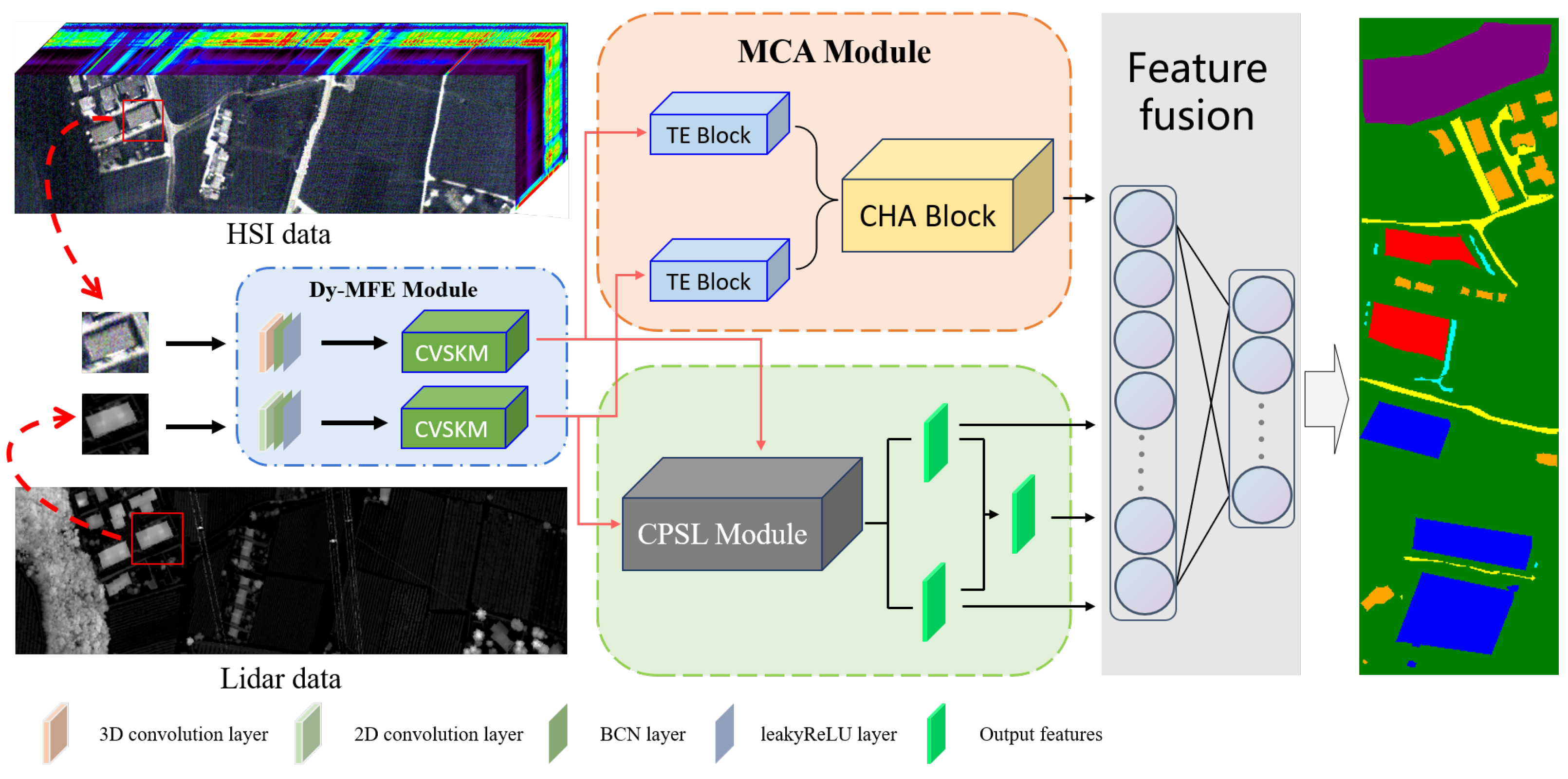
In this section, we will elaborate on the details of TCPSNet, primarily focusing on four components: dynamic multi-scale feature extraction module (Dy-MFEM), multimodal cross-attention module (MCAM), cross-pseudo-siamese learning module (CPSLM) as well as the multimodal mixed fusion method, shown in Figure 1. Using the fusion of HSI and LiDAR data as an example, firstly, we use Dy-MFEM to extract the shallow features of the two kinds of data, respectively, and then we use a four-branch network to extract the deep features of HSI and LiDAR data using the MCAM and CPSLM, respectively, in which the two outputs obtained from the MCAM are directly involved in the decision-level fusion, and the two outputs obtained from the CPSLM will first undergo a feature-level fusion to obtain a new feature, and then the three outputs including the new feature are fused together with the two outputs of the MCAM at the decision level, and finally the classification results are generated by decision-level fusion.

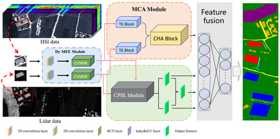
Figure 1. The main structure of TCPSNet.

3.2. Dynamic Multi-Scale Feature Extraction Module

First, we use 3D-CNN to extract the spectral and spatial information of HSI data, and 2D-CNN to extract the elevation information of LiDAR data. Meanwhile, this study added a batch channel normalization (BCN) layer and a leaky rectified linear unit (Leaky ReLU) layer after the convolutional layer. BCN combines the advantages of batch normalization (BN) and layer normalization (LN) to adaptively exploit channel and batch correlation. Specifically, it normalizes the spatial dimensions (N, H, W) and channel dimensions (C, H, W), and after normalization, the BCN merges the results using adaptive parameters to avoid the singularity vanishing problem caused by channel normalization. The Leaky ReLU is an improved linear unit that prevents the gradient descent problem by maintaining linearity in the non-negative part and introducing a small slope in the negative part. Then, we designed the combined variable selectivity kernel module (CVSKM) based on the feature that neighboring features have similarity, using the method of adaptively changing the spatial sensing domain in order to enable the network to pay more attention to the wide range of background information of remote sensing images.

Figure 2 shows the structure of the CVSKM. As can be seen in the right portion of the image, we employed 1 × 1 convolution to integrate the data and large kernel and atrous convolution to stimulate the rapid development of the sensory domain. After that, we split the features under various receptive domains and use a pooling process to determine the closeness relationship between the features.

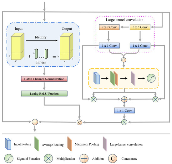
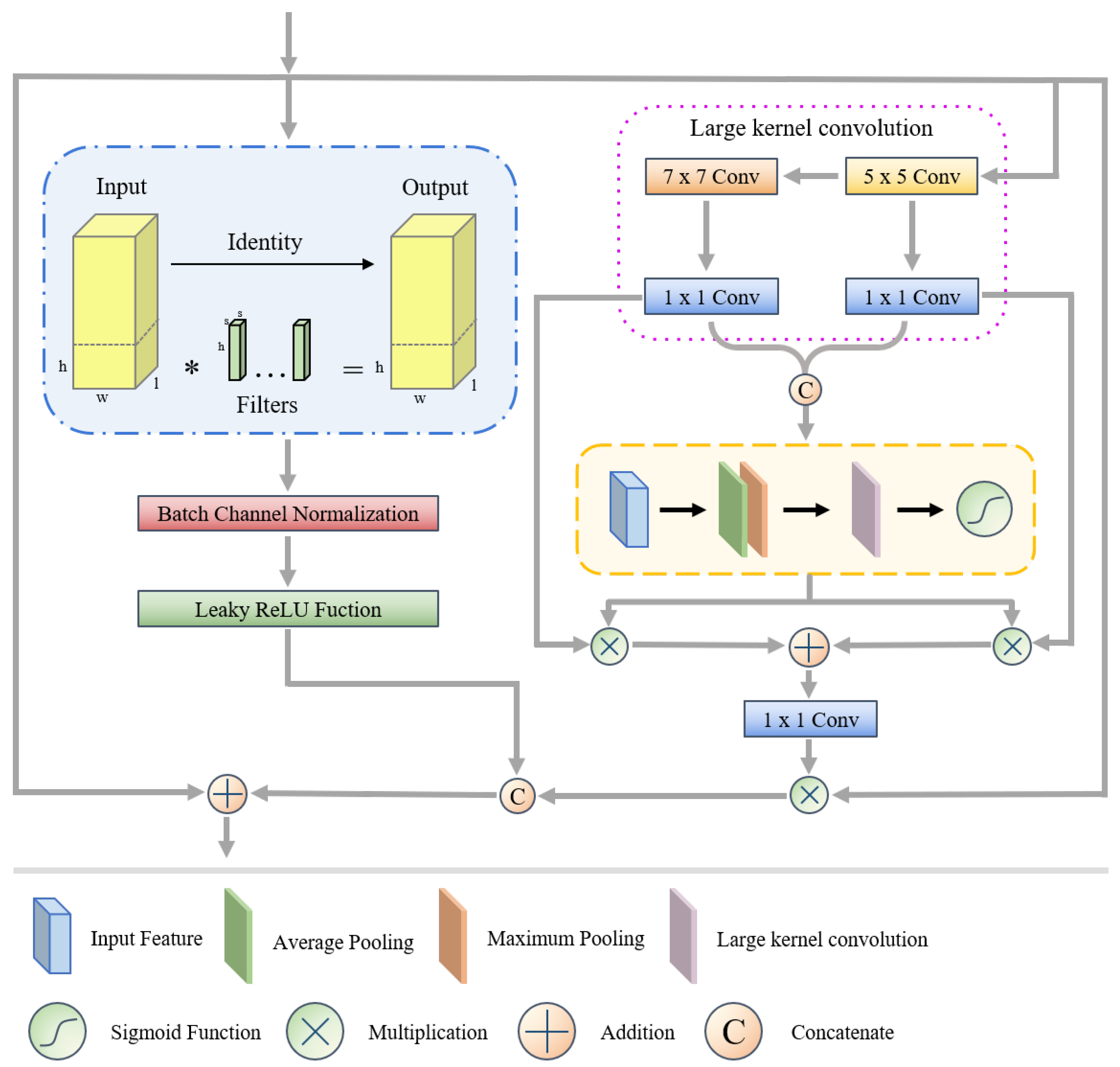
Figure 2. Structure of combination variable selectivity kernel module. Where * represent the execution of the multiplication operation.

Figure 2. Structure of combination variable selectivity kernel module. Where * represent the execution of the multiplication operation.

$$\begin{array}{c}\hfill \begin{array}{c}\hfill \tilde{F}=\left\{\widetilde{F_1};\widetilde{F_2};\dots ;\widetilde{F_i}\right\}\end{array}\end{array}$$

(1)

$$\begin{array}{c}\hfill \begin{array}{cc}\hfill & A{M}_{avg}=P_{avg}\left(\tilde{F}\right)\hfill \\ & A{M}_{max}=P_{max}\left(\tilde{F}\right)\hfill \end{array}\end{array}$$

(2)

$$\begin{array}{c}\hfill \begin{array}{c}\hfill \widetilde{AM}=\sigma \left(\delta (A{M}_{avg};A{M}_{max})\right)\end{array}\end{array}$$

(3)

Among them, $\widetilde{F_i}$ represents features at different scales, $\tilde{F}$ represents the result after cascading the features, $A{M}_{avg}$ and $A{M}_{max}$ are the average and maximum pooled spatial feature descriptors, where channel-based average and maximum pooling were denoted as $P_{avg}$(·) and $P_{max}$(·), $\sigma$(·) represents the softmax function, $\delta$(·) represents 2D convolution and $\widetilde{AM}$ represents the spatial selection mask obtained from the spatial attention mapping via the softmax function.

Next, we employ matching spatial masks to weight the decomposed large kernel sequence features, and a 1 × 1 convolution is used to fuse them.

$$\begin{array}{c}\hfill \begin{array}{c}\hfill {\displaystyle Y_i=\varphi \left(\sum _{i=1}^N\left(\widetilde{A{M}_i}\widetilde{F_i}\right)\right)}\end{array}\end{array}$$

(4)

Among them, $\varphi$(·) represents 1 × 1 convolution, $\widetilde{A{M}_i}$ represents the individual spatial selection mask and $Y_i$ represents the final attention feature obtained.

Meanwhile, we introduce a method called partial convolution, which selects certain channels for feature extraction while leaving others unaltered. This action was conducted in response to the difficulty presented by 3D convolutions, which produce a large number of channels and consequently redundant features. Regarding the LiDAR branch, we purposefully avoided using partial convolution in favor of stacking convolutional layers in order to prevent gradient vanishing.

3.3. Multimodal Cross-Attention Module

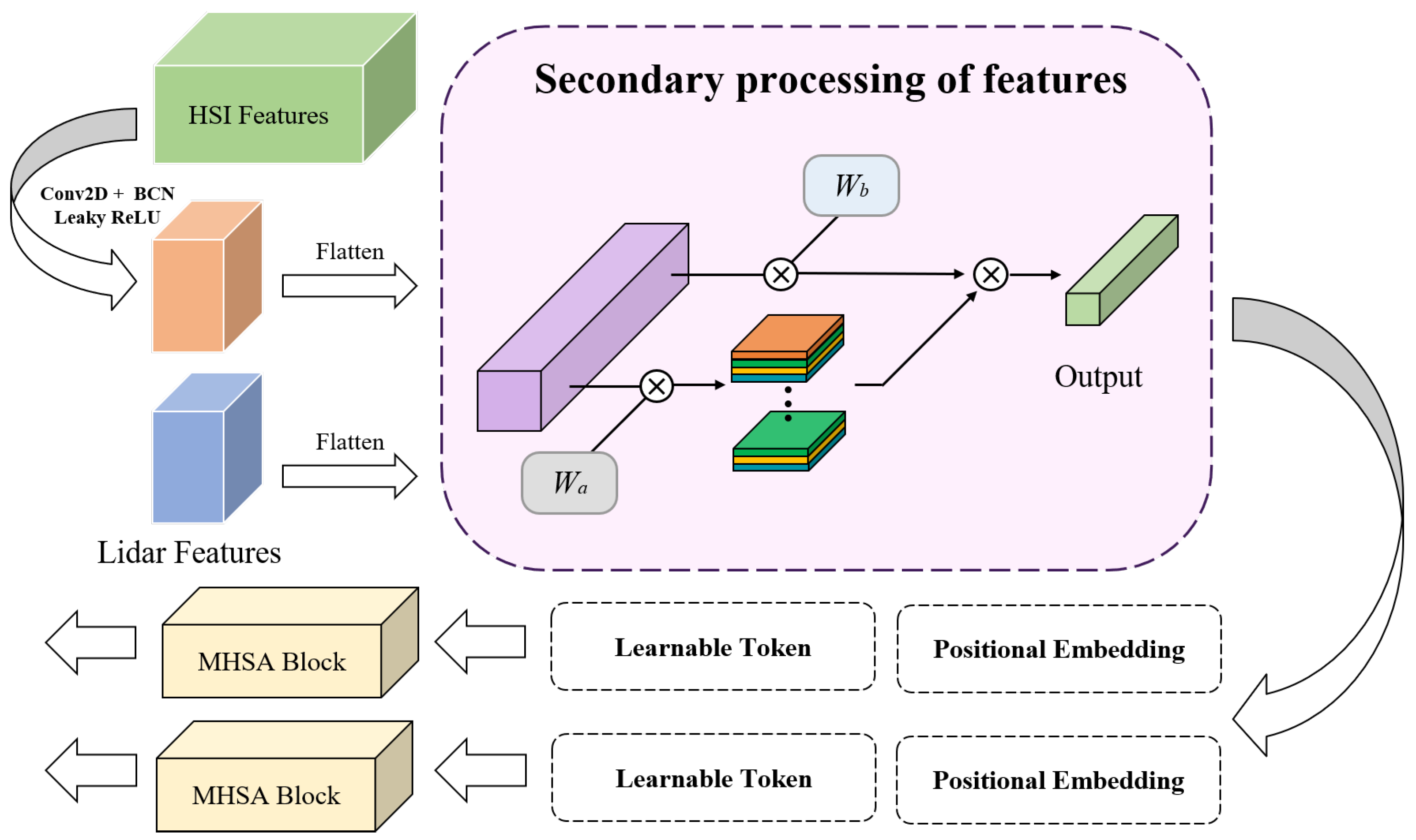
As illustrated in Figure 3, we first apply 2D convolution to the hyperspectral data in order to achieve parity between the sizes of the features in the hyperspectral and LiDAR data. Subsequently, the feature maps undergo flattening into feature vectors and transposition, resulting in the representation of $C^{m1}$ and $C^{m2}$. Following that, two sets of normally distributed learnable weights $W_a^{m1}$,$W_b^{m1}$ and $W_a^{m2}$,$W_b^{m2}$ can be used to obtain the secondary processed features. The entire procedure can be summed up as follows:

$$\begin{array}{c}\hfill \begin{array}{c}\hfill T^{m1}=\sigma \left(T\left(C^{m1}{W}_a^{m1}\right)\right)C^{m1}{W}_b^{m1}\\ \hfill T^{m2}=\sigma \left(T\left(C^{m2}{W}_a^{m2}\right)\right)C^{m2}{W}_b^{m2}\end{array}\end{array}$$

(5)

where $\sigma$(·) is the softmax function, T(·) is the transpose function, $m1$ and $m2$ represent the remote sensing data of two modalities, namely hyperspectral data and LiDAR data, $T^{m1}$ and $T^{m2}$ are the final labeled features obtained.

Figure 3. Proposed multimodal cross-attention module for deep feature fusion. First, convolution is performed on the hyperspectral data to achieve their feature size equal to that of the lidar data. Second, the multi-source remote sensing data are subjected to feature secondary processing. Third, we add positional embedding and learnable markers to features. Finally, the output is passed into the MHSA block for depth information capture. Additionally, the multiplication symbols in the figure all represent the execution of the multiplication operation.

Immediately after that, we embed the feature tokens representing the location information and the learnable classification tokens for completing the classification task into the labeled features; then, we can use the Transformer encoder to learn the features, and with the powerful context extraction capability of the Multihead Self-Attention (MHSA) block, we can construct a global feature map of the remote sensing data from multiple sources.

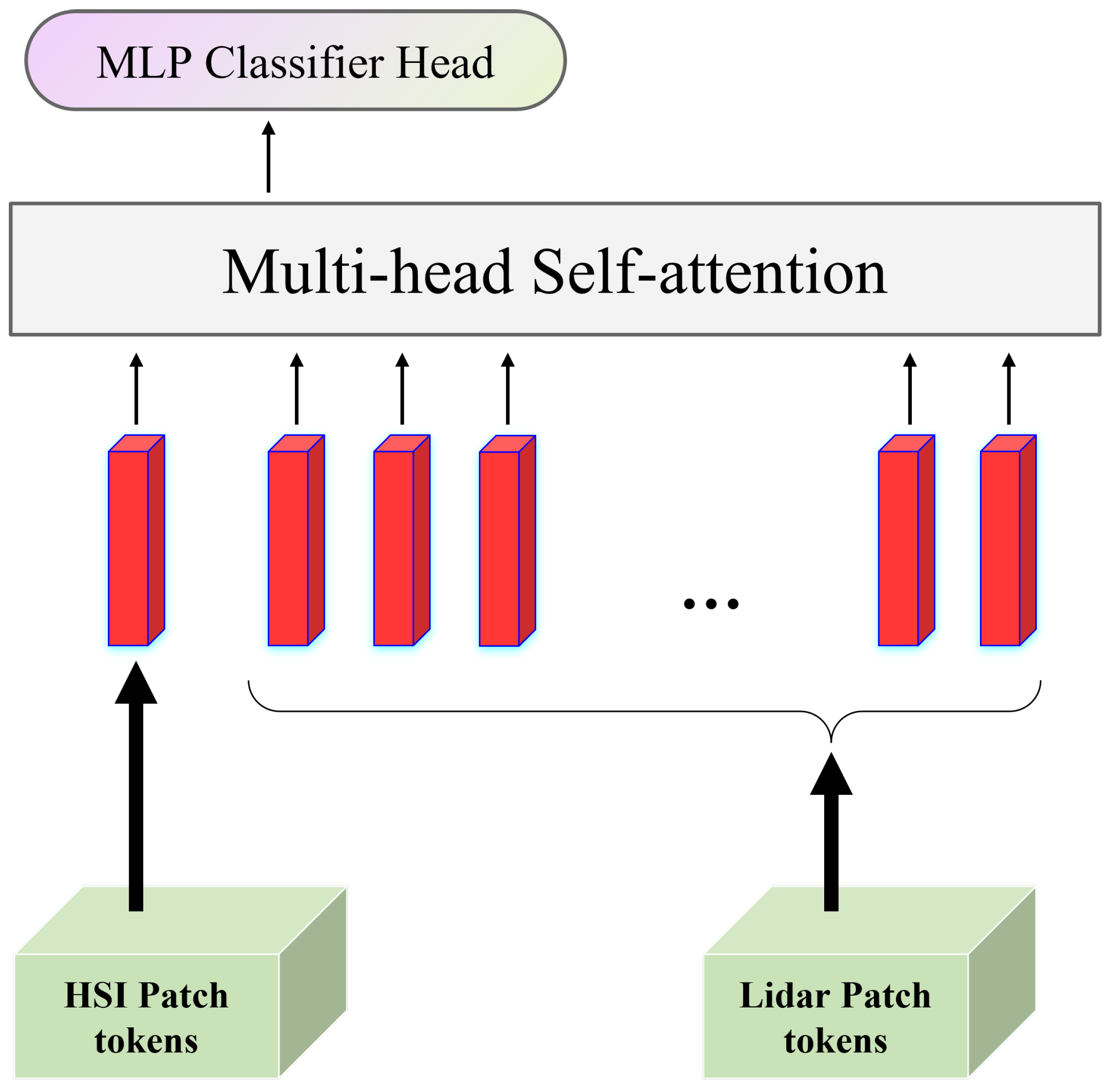
Then, in order to fuse multimodal information, we designed the cross-head attention (CHA) module. Using the MHSA as a guide, we tried to use the data from one modality as the learnable classification tokens of the data from another modality for self-attention learning. With the help of this module’s potent inter-data interaction capabilities, we were able to identify numerous correlations between the features of multiple sources. Figure 4 illustrates the module’s detailed algorithmic flow.

Figure 4. Structure of cross-head attention module. HSI data as a learnable categorical marker for Lidar data for self-attention learning and finally using MLP Classifier Head for result output.

3.4. Cross-Pseudo-Siamese Learning Module

A Transformer is a powerful tool for modeling contextual information, but it is also important to control the local information. Unfortunately, current research on CNN-based multi-source remote sensing data methods typically falls short in addressing the issue of high coupling between heterogeneous data and the inability to achieve multimodal data sharing on high-level features. As a result, we created CPSLM, the structure of which is depicted Figure 5.

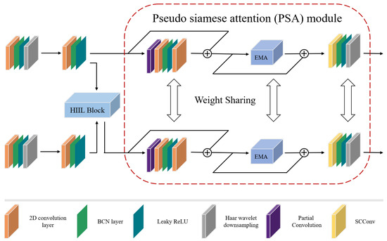
Figure 5. Structure of cross-pseudo-siamese learning module. The upper branch is a branch of HSI and the lower branch is a branch of LiDAR. The plus signs in the figure all represent the execution of the summing operation.

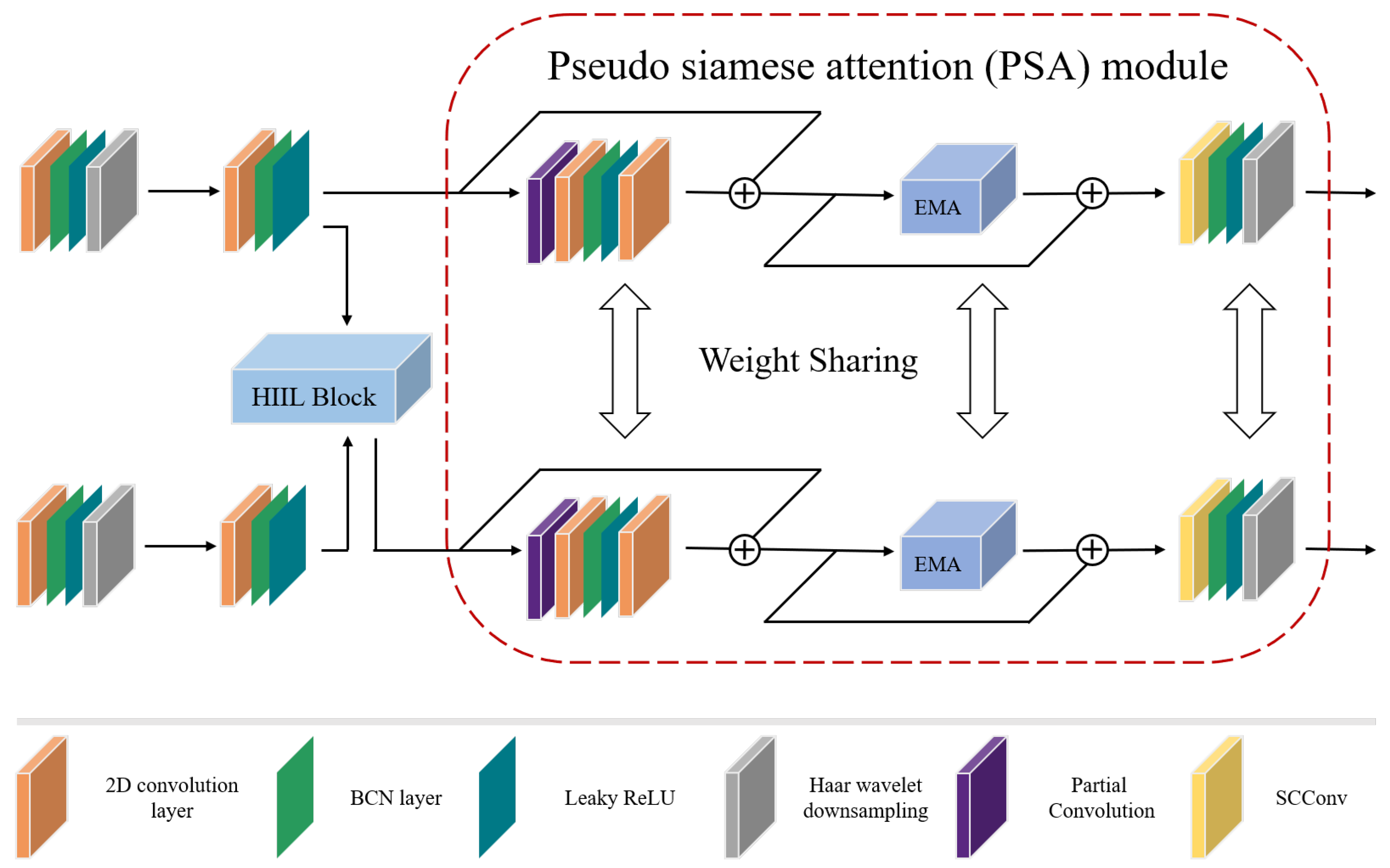
We use the convolutional layer, BCN layer, Leaky ReLU layer and the Haar wavelet downsampling (HWD) layer to achieve the extraction of spectral, spatial and elevation characteristics for HSI and LiDAR data during the deep feature extraction stage. It is important to pay attention to the HWD layer. While maximum pooling is used in most conventional down-sampling operations, it loses some important information when too many features are pooled in the local neighborhood for feature classification of remote sensing images. To mitigate this, HWD combines representational feature learning with lossless feature coding, which can partially restore the original components of each modality. Next, unlike CHA, we create the heterogeneous information-induced learning (HIIL) module, whose structure is depicted in Figure 6. The HIIL module is capable of fusing heterogeneous information from different sources while maintaining the 2D structure of the image.

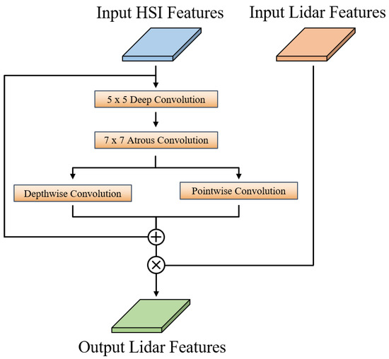
Figure 6. Structure of heterogeneous information-induced learning module. The plus and multiplication signs in the figure represent addition and multiplication operations, respectively.

We design the pseudo-siamese attention (PSA) module to further fuse the multimodal information. First, we use partial convolution to accelerate the extraction of the coupled features. Secondly, we use the EMA module to aggregate the spatial structural information at multiple scales for the long-range relations obtained by HIIL. Finally, we use the SC convolution to prevent both spatial and channel redundancy. We also use the weight sharing strategy in every layer of the module to fully couple the multimodal features. This yields the appearance of a siamese neural network and also helps to reduce the number of network parameters.

3.5. Fusion of Multi-Source Data

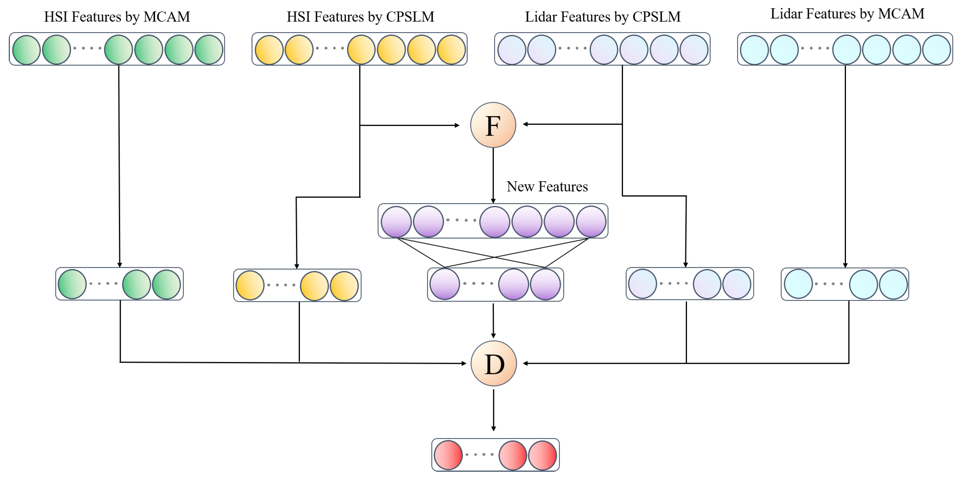
In order to obtain greater classification accuracy, the multimodal combined fusion method developed in this study combines feature-level and decision-level fusion. It is shown as follows:

$$\begin{array}{c}\hfill \begin{array}{cc}\hfill & Y=D\left\{F_1(X_{m1};W_1),F_2(X_{m2};W_2),F_3(X_{m1};W_3),\right.\hfill \\ & \left.F_4(X_{m2};W_4),F_5(M(X_{m1},X_{m2});W_5);U\right\}\hfill \end{array}\end{array}$$

(6)

Among them, $X_{m1}$ and $X_{m2}$ represent remote sensing data of two modalities, respectively, while $F1$(·) and $F2$(·) represent the output layer of the MCAM, $F3$(·) and $F4$(·) represent the output layer of the CPSLM, $F5$(·) represents the output layer of feature-level fusion, M(·) represents the execution of feature-level fusion, D(·) represents the execution of decision-level fusion, $W1$, $W2$, $W3$, $W4$, and $W5$ represent the connection weights of each output layer, U is the fusion weight for decision-level fusion, and its specific structure is shown in Figure 7.

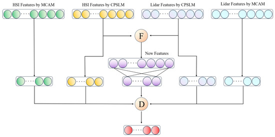
Figure 7. Structure of the fusion module. F represent feature-level fusion and D represent decision-level fusion. New feature from feature-level fusion of HSI and LiDAR.

For feature-level fusion, we use the summation method, the maximum value method and the PagFM function method, which are three fusion strategies. Among them, the PagFM function method is often used to mitigate the overshooting phenomenon generated when fusing high-resolution details and low-frequency contexts. Therefore, we try to add it into the fusion of multi-source remote sensing data to induce the heterogeneous information to be fused effectively. The computational procedure for all feature-level fusion is as follows:

$$\begin{array}{c}\hfill \begin{array}{cc}\hfill & M_S(X_{m1},X_{m2})=X_{m1}+X_{m2}\hfill \\ & M_m(X_{m1},X_{m2})=max(X_{m1},X_{m2})\hfill \\ & M_p(X_{m1},X_{m2})=PagFM(X_{m1},X_{m2})\hfill \end{array}\end{array}$$

(7)

Among them, $M_S$(·), $M_m$(·) and $M_p$(·) represent three feature level fusion methods, respectively. $max$(·) and $PagFM$(·) represent the maximum function and PagFM function, respectively.

We tried allocating additional computational resources to more challenging categories to identify due to the small number of land samples in some categories from remote sensing land classification jobs.Thus, unlike typical deep learning research that employs cross-entropy loss to forecast models, we devised a joint learning method based on remote sensing data (RSJLM). It is defined as follows:

$$\begin{array}{c}\hfill \begin{array}{c}\hfill DL=1-{\displaystyle \frac{2{\sum }_{i=1}^N{y}_i\widehat{y_i}}{{\sum }_{i=1}^N{y}_i+{\sum }_{i=1}^N\widehat{y_i}}}\end{array}\end{array}$$

(8)

The above equation is the formula for Dice Loss, where $y_i$ and $\widehat{y_i}$ represent the ground truth label and predicted value for each pixel i, respectively. The total number of pixels is N, and its size is the batch size multiplied by the total number of pixels in a single image.

$$\begin{array}{c}\hfill \begin{array}{c}\hfill FL=-{\alpha }_t{(1-p_t)}^{\gamma }log\left(p_t\right)\end{array}\end{array}$$

(9)

The above equation provides a detailed introduction to the focal loss formula, where ${\alpha }_t\in [0,1]$,$\gamma \in [0,5]$ are the variable weight parameters and $P_t$ represents the predicted value of class t.

$$\begin{array}{c}\hfill \begin{array}{c}\hfill Loss=\alpha DL-log\left(FL\right)\end{array}\end{array}$$

(10)

The loss function used in the RSJLM proposed in this article is shown in the above equation, where DL represents Dice loss, FL represents focal loss and $\alpha$ is a weight parameter.

4. Experiment and Analysis

4.1. Datasets

The Trento, Houston 2013 and Augsburg datasets are three of the prime multi-source remote sensing datasets that this study picked to verify the efficacy of the proposed method. The following will show the basic information of the three datasets, where the ground truth map denotes the distribution of all ground truth sample labels. The training and test sets are constructed by randomly selecting the training and test samples according to a certain number of samples, and the same training and test sets are used for the same dataset in all experiments except for the sample analysis experiment. The distribution of training and testing sample numbers is shown in Table 1.

Table 1. Training and test sample numbers for Trento, Houston and Augsburg datasets.

	Trento Dataset			Houston 2013 Dataset			Augsburg Dataset
Class	Class Name	Training.	Test.	Class Name	Training.	Test.	Class Name	Training.	Test.
C01	Apple Trees	129	3905	Healthy Grass	198	1053	Forest	675	12,832
C02	Buildings	125	2778	Stressed Grass	190	1064	Residential Area	1516	28,813
C03	Ground	105	374	Synthetic Grass	192	505	Industrial Area	192	3659
C04	Woods	154	8969	Trees	188	1056	Low Plants	1342	25,515
C05	Vineyard	184	10,317	Soil	186	1056	Allotment	28	547
C06	Roads	122	3052	Water	182	143	Commercial Area	82	1563
C07				Residential	196	1072	Water	76	1454
C08				Commercial	191	1053
C09				Road	193	1059
C10				Highway	191	1036
C11				Railway	181	1054
C12				Parking Lot1	194	1041
C13				Parking Lot2	184	285
C14				Tennis Court	181	247
C15				Running Track	187	473
-	Total	819	29,395	Total	2932	12,197	Total	3911	74,383

4.1.1. Trento Dataset

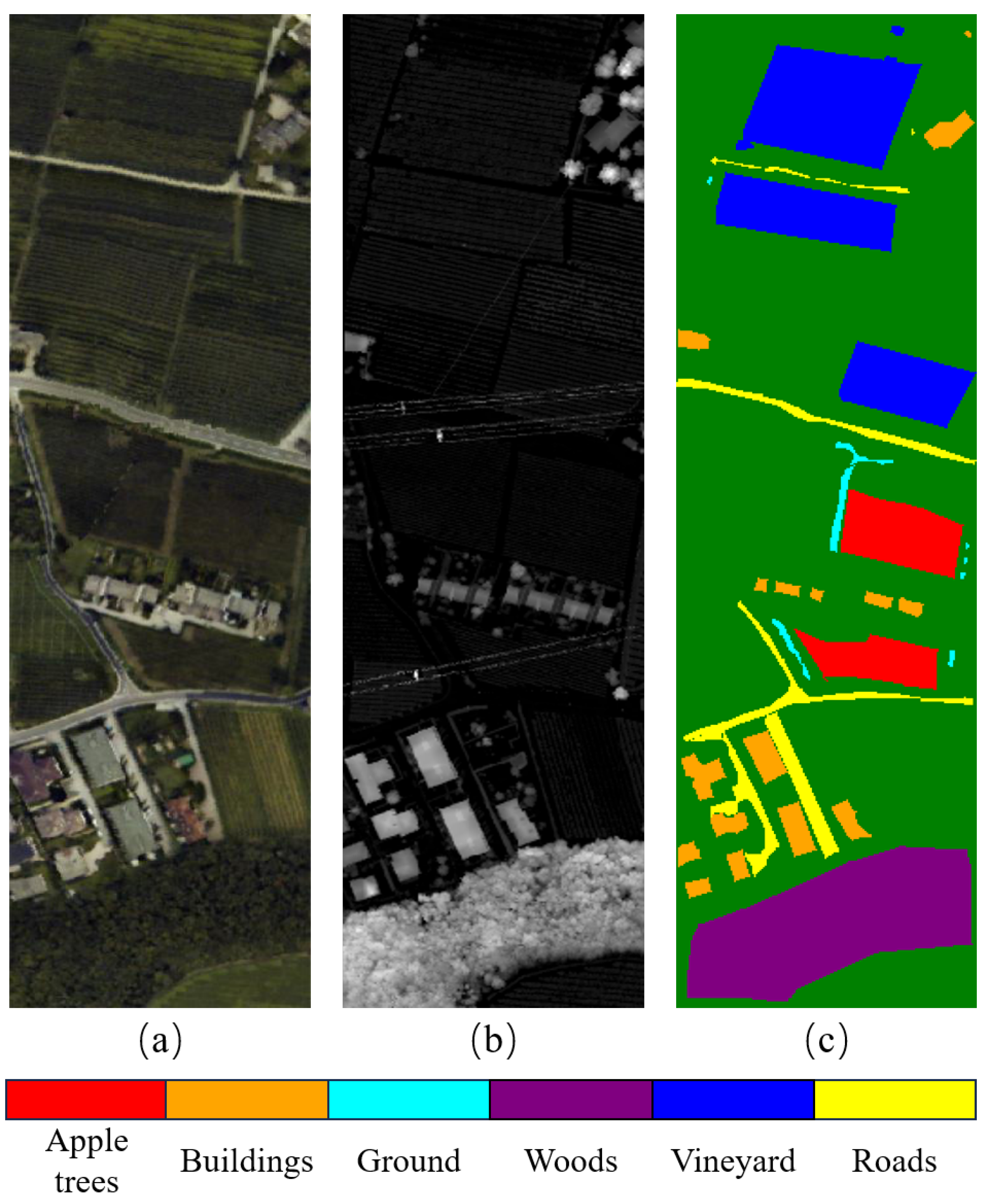
Trento dataset [38] was acquired in a rural area in the south of Trento, Italy. The LiDAR data were acquired with the Optech ALTM 3100EA sensor, and the hyperspectral data were acquired with the AISA Eagle sensor, containing 63 spectral bands, with a spectral resolution of 9.2 nm, and a wavelength range of 0.42 $\mathsf{\mu }$m to 0.99 $\mathsf{\mu }$m. The two datasets cover the same area, the image size is 166 × 600 pixels and the spatial resolution is 1 m. Six different classes and corresponding ground samples are included, and the detailed information is shown in Figure 8.

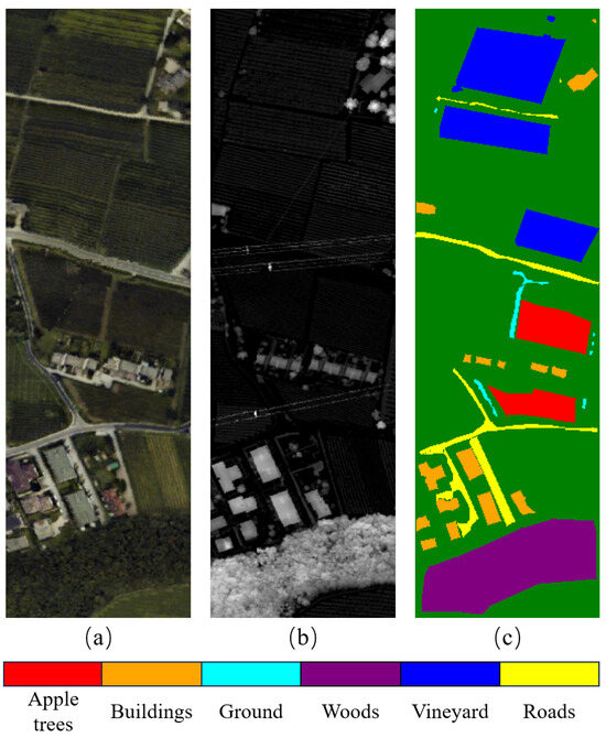
Figure 8. Trento dataset and all its feature classes. (a) Pseudo-color composite images in the 20th, 15th and 5th bands based on hyperspectral data. (b) Grayscale image for LiDAR-based DSM. (c) Ground truth map.

4.1.2. Houston 2013 Dataset

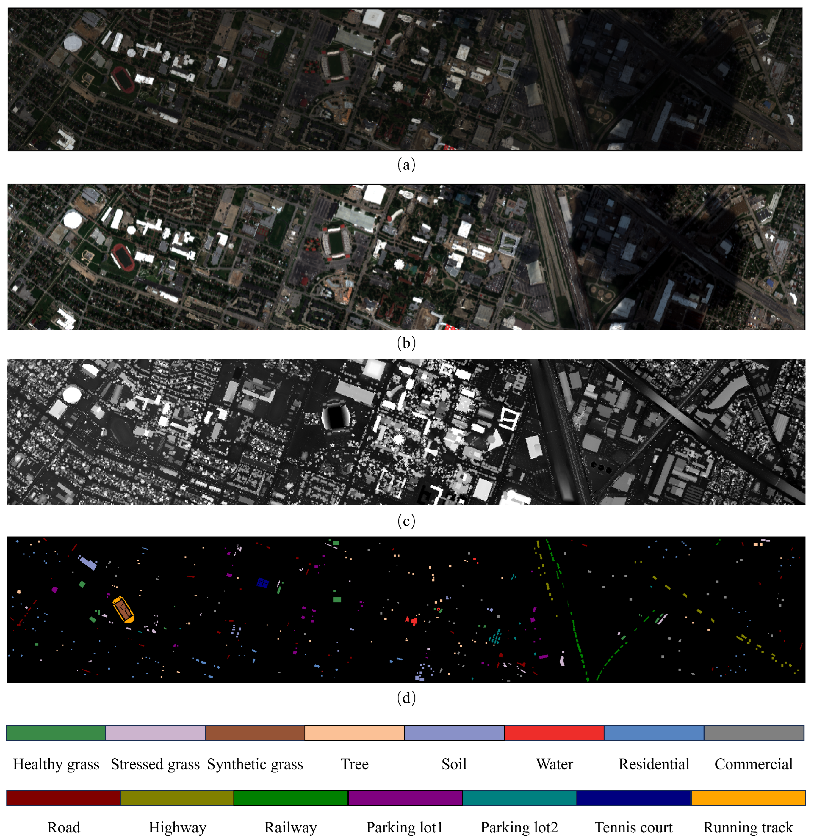
The Houston 2013 Dataset [39,40] was provided by the Institute for Earth Science and Remote Sensing (IEEE GRSS) in the 2013 Data Fusion Competition https://hyperspectral.ee.uh.edu/?page_id=459/(accessed on 5 July 2024). The region contains the university of Houston campus and surrounding areas, collected in 2012, including HSI data, multispectral images (MSI) data, and LiDAR data, covering the same area and all consisting of 349 × 1905 pixels, with a spatial resolution of 2.5 m. HSI contains 144 bands and MSI contains 8 bands in the wavelength range of 0.38–1.05 $\mathsf{\mu }$m. The dataset consists of 15 different classes and corresponding ground samples, detailed information of which is shown in Figure 9.

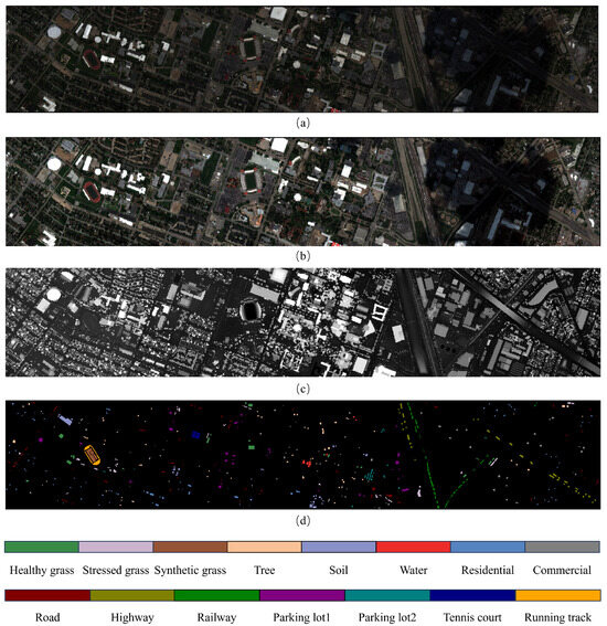
Figure 9. Houston dataset and all its feature classes. (a) Pseudo-color composite images in the 59th, 40th and 23th bands based on hyperspectral data. (b) Pseudo-color composite images of 3rd, 2nd and 1st bands based on multispectral data. (c) Grayscale image for LiDAR-based DSM. (d) Ground truth map.

4.1.3. Augsburg Dataset

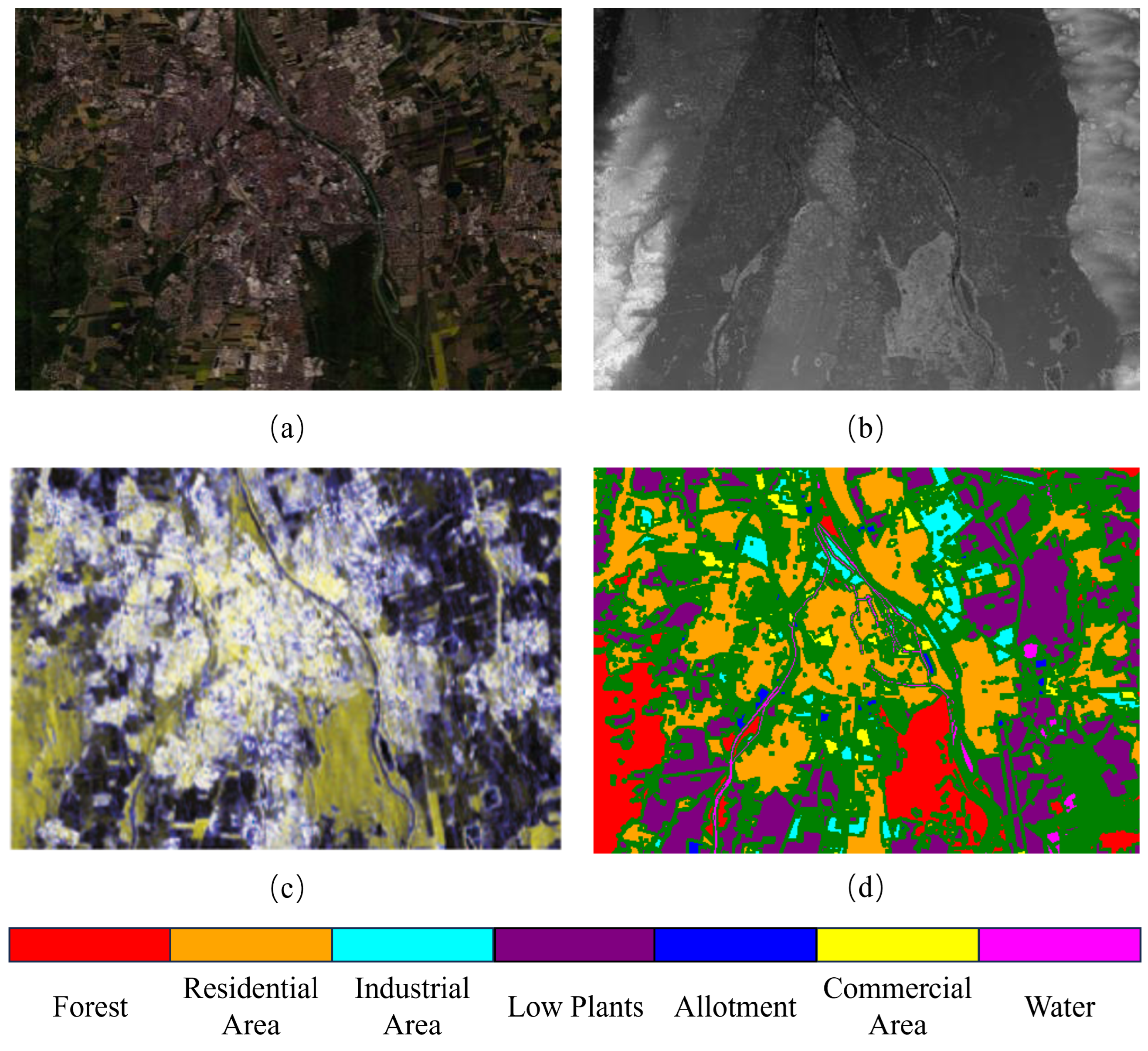
The Augsburg dataset [41] was acquired in the city of Augsburg, Germany. A total of three remote sensing data types, HSI, SAR and DSM, are included, in which HSI is obtained by DAS-EOC HySpex located over the city and contains 180 bands ranging from 0.4 $\mathsf{\mu }$m to 2.5 $\mathsf{\mu }$m, SAR data are collected from the Sentinel-1 platform and contain four bands, which denote the VV intensity, the VH intensity, the real component and the imaginary component, and the DSM data are obtained by DLR-3 K, and all the data cover the same area and are uniformly down-sampled to a spatial resolution of 30 m with image size of 332 × 485 pixels. Meanwhile, the dataset contains 7 different classes and corresponding ground samples, and the detailed information is shown in Figure 10.

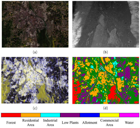
Figure 10. Augsburg dataset and all its feature classes. (a) Pseudo-color composite images in the 20th, 15th and 10th bands based on hyperspectral data. (b) Grayscale image for LiDAR-based DSM. (c) Pseudo-color composite images based on SAR data. (d) Ground truth map.

4.2. Experimental Settings

4.2.1. Evaluation Indicators

Three widely used classification evaluation indicators in the industry, namely overall accuracy (OA), average accuracy (AA) and Kappa coefficient, are primarily used to accurately assess the performance of the method proposed in this article.

OA reflects the difference between the classification results of all test samples and the true label value with the following formula:

$$\begin{array}{c}\hfill \begin{array}{c}\hfill OA={\displaystyle \frac{{\displaystyle \sum _{i=1}^C{T}_i}}{{\displaystyle \sum _{i=1}^C{N}_i}}}\end{array}\end{array}$$

(11)

Among them, $T_i$ is the number of correctly categorized samples in category i, $N_i$ is the total number of samples in category i, and C denotes the number of categories to be categorized.

AA reflects the average of the classification accuracies of all categories, which is calculated as follows:

$$\begin{array}{c}\hfill \begin{array}{c}\hfill {\displaystyle AA=\frac{1}{C}\sum _{i=1}^C\frac{T_i}{N_i}}\end{array}\end{array}$$

(12)

The Kappa coefficient is used to test the consistency and assess classification performance with the following formula:

$$\begin{array}{c}\hfill \begin{array}{c}\hfill M={\displaystyle \frac{{\displaystyle \sum _{i=1}^C{x}_i{y}_i}}{n^2}}\end{array}\end{array}$$

(13)

$$\begin{array}{c}\hfill \begin{array}{c}\hfill Kappa={\displaystyle \frac{OA-M}{1-M}}\end{array}\end{array}$$

(14)

Among them, $x_i$ is the actual number of samples in category i, $y_i$ is the predicted number of samples in category i and n is the total number of samples.

4.2.2. Configurations

All the experiments of the proposed method and other selected comparative methods in this study are implemented in PyTorch 1.12.0 deep learning framework using a server with Intel Xeon Bronze 3106 as the server’s central processor, 128 GB of RAM. The image processor is NVIDIA GeForce RTX 3090 with 24 GB of video memory. The optimizer is selected as Adam optimizer, the batch size is 64, the number of iterations epoch is set to 100 and the learning rate is set to 0.001.

4.3. Parameter Analysis

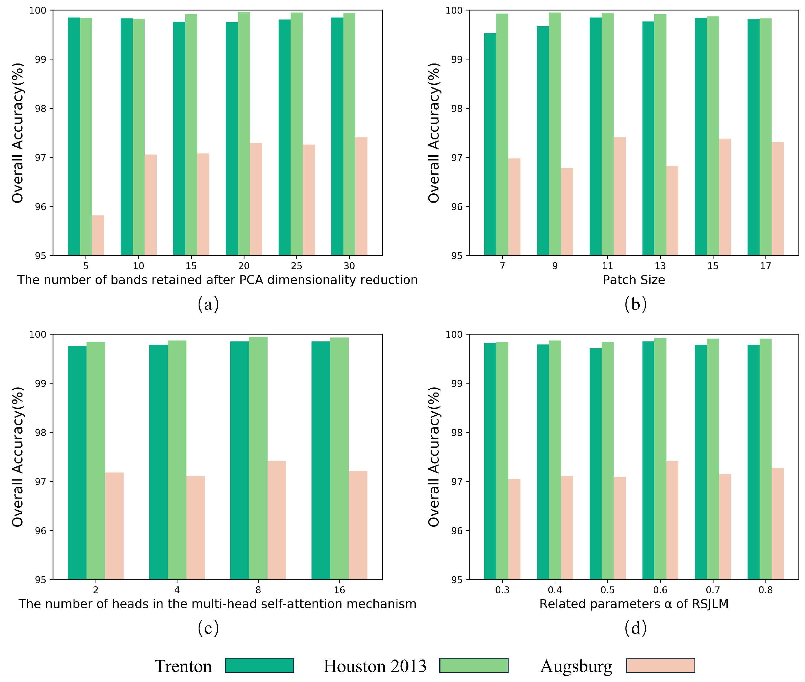
In this study, a detailed parametric analysis was conducted to investigate the effect of each hyperparameter of TCPSNet on model training. The hyperparameters we selected include the number of bands retained after principal component analysis (PCA) dimensionality reduction, the patch size, the number of heads in the multi-head self-attention mechanism and the related parameter $\alpha$ of RSJLM. Candidate sets of parameter values are identified with reference to the relevant literature [28,30]. Each of our experiments only changes the value of one of the hyperparameters, while ensuring that the values of the other three hyperparameters are fixed, and the analysis results are shown in Figure 11.

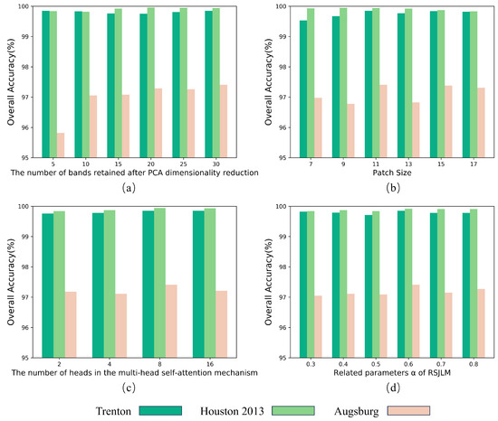
Figure 11. Influence of different parameters on the overall accuracy in three datasets. (a) The number of bands retained after PCA dimensionality reduction. (b) Patch size. (c) The number of heads in the multi-head self-attention mechanism. (d) Related parameters $\alpha$ of RSJLM.

In terms of the dataset, the Augsburg dataset has a significant change in OA when the hyperparameters are changed, while the other two datasets have almost no change. This phenomenon may be due to the fact that the Augsburg dataset has far more sample data than the other two datasets, and the model needs to be more carefully tuned to achieve optimal performance, while small changes in the hyperparameters may lead to significant fluctuations in the model’s performance.

In terms of parameter selection, we identified the optimal values for all four hyperparameters:

4.3.1. The Number of Bands Retained after PCA Dimensionality Reduction

We select the number of bands retained after dimensionality reduction from the candidate set {5, 10, 15, 20, 25, 30}. From Figure 11a, we can see that, in general, the OA improves with the increase in the number of bands, and the optimal parameter is 30 for Trento and Augsburg data, and 20 for Houston, and for convenience, the number of bands in the subsequent experiments we uniformly set to 30.

4.3.2. Patch Size

We select the values of the patch size from the candidate set {7, 9, 11, 13, 15, 17}. As can be seen from Figure 11b, the optimal OA was achieved with the patch size of 11 in three datasets.

4.3.3. The Number of Heads in The Multi-Head Self-Attention Mechanism

We select the number of attention heads from the candidate set {2, 4, 8, 16}. The experimental results are shown in Figure 11c, and it can be seen that the optimal number of self-attention heads is 8 for all the three datasets.

4.3.4. Related Parameters $\alpha$ of RSJLM

We select the values of the parameter $\alpha$ from the candidate set {0.3, 0.4, 0.5, 0.6, 0.7, 0.8}, and the results of the experiments are shown in Figure 11d, which shows that the optimal value of $\alpha$ is 0.6 for all the three datasets.

4.4. Comparison to State-of-the-Art Methods

A number of methods have been evaluated using the Trento, Houston and Augsburg datasets in the majority of the research that has been conducted on multi-source remote sensing data fusion. To evaluate the performance of our proposed method, we have chosen a number of representative methods and carried out comparison tests. Among these techniques are CoupledCNN [23], M2FNet [32], DSHF [28], CALC [17], 2D-CNN [13] and 3D-CNN [14]. Among them, the 2D-CNN and 3D-CNN methods use only hyperspectral data for classification, while all other networks use multi-source remote sensing data. And all methods’ settings are set in accordance with the original text’s description.

4.4.1. Quantitative Results and Analysis

Based on three datasets, Table 2, Table 3 and Table 4 display the accuracy for each category, namely OA, AA and Kappa coefficients. The optimal outcomes in each table are in bold. As may be observed, the method proposed in this article has greatly advanced the above previous methods. Comparing the three datasets to the methods used in recent years, the OA has increased by 0.89%, 4.19% and 4.1%. Additionally, the AA has grown by 1.68%, 3.94% and 19.7%, in that order. Moreover, there have been increases in the Kappa coefficient of 1.11%, 4.22% and 5.67%, respectively.

Table 2. Classification accuracies (%) and Kappa coefficients of different models on the Trento dataset.

	2D-CNN	3D-CNN	M2FNet	CALC	DSHF	CoupledCNN	Proposed
Apple Trees	94.29	94.21	99.23	98.13	99.62	99.54	99.90
Buildings	85.24	87.19	98.38	99.24	99.68	97.37	99.24
Ground	83.69	89.30	90.37	81.55	97.86	97.59	100.00
Wood	99.59	99.91	99.59	100.00	98.53	100.00	100.00
Vineyard	99.02	98.60	100.00	99.84	100.00	100.00	100.00
Roads	79.03	78.93	93.48	90.20	90.43	92.40	97.77
OA (%)	94.99	95.18	98.82	98.44	98.74	98.87	99.85
AA (%)	90.14	91.36	96.84	94.94	97.76	97.82	99.49
Kappa × 100	93.29	93.58	98.42	97.91	98.31	98.48	99.58

Table 3. Classification accuracies (%) and Kappa coefficients of different models on the Houston dataset.

	2D-CNN	3D-CNN	M2FNet	CALC	DSHF	CoupledCNN	Proposed
Healthy Grass	96.30	98.10	82.24	82.05	81.20	93.83	98.39
Stressed Grass	95.77	98.68	98.68	98.59	98.78	97.27	100.00
Synthetic Grass	96.04	99.80	94.65	94.46	100.00	96.24	99.80
Trees	90.63	89.30	96.40	97.35	99.81	100.00	99.81
Soil	98.96	99.72	99.43	100.00	100.00	100.00	100.00
Water	97.90	99.30	95.80	97.90	84.62	95.80	100.00
Residential	74.91	90.58	92.07	90.21	83.49	93.84	99.91
Commercial	53.00	74.45	92.78	91.45	69.33	95.63	100.00
Road	76.49	79.60	95.00	89.52	39.81	89.14	99.62
Highway	74.81	52.41	89.67	94.88	80.02	98.65	100.00
Railway	53.80	89.28	92.13	99.62	82.54	97.25	99.91
Parking Lot1	51.87	80.79	92.80	87.80	94.91	90.97	98.46
Parking Lot2	83.86	94.39	90.18	85.96	83.51	89.12	98.25
Tennis Court	99.60	96.36	100.00	100.00	96.76	97.57	100.00
Running Track	98.52	100.00	99.15	100.00	99.79	99.79	100.00
OA (%)	79.23	87.14	93.53	93.50	91.79	95.73	99.92
AA (%)	82.83	89.52	94.07	93.99	92.58	95.67	99.61
Kappa × 100	77.52	86.04	92.98	92.94	91.09	95.36	99.58

Table 4. Classification accuracies (%) and Kappa coefficients of different models on the Augsburg dataset.

	2D-CNN	3D-CNN	M2FNet	CALC	DSHF	CoupledCNN	Proposed
Forest	97.20	94.97	92.25	90.46	96.34	98.59	99.02
Residential Area	96.79	98.20	96.73	96.13	94.10	98.36	99.40
Industrial Area	87.87	75.62	76.89	91.38	67.18	63.11	87.65
Low Plants	96.51	97.81	94.57	95.61	97.48	95.33	98.99
Allotment	1.10	35.65	23.33	25.81	51.24	51.05	90.49
Commercial Area	3.58	17.15	1.16	1.65	0.08	8.55	60.84
Water	38.93	50.89	39.55	53.02	0.27	32.58	71.80
OA (%)	92.53	93.31	90.61	91.43	90.21	92.13	97.41
AA (%)	60.28	67.18	60.64	64.87	58.05	63.94	86.88
Kappa × 100	89.22	90.31	86.43	87.71	85.77	88.60	95.98

Simultaneously, we demonstrate that methods that solely rely on HSI data for classification have major drawbacks when compared to multi-source data classification methods for the majority of datasets. Regarding classification accuracy, the method proposed in this paper has enhanced the residential category of Houston by 6.07% over the methods used in recent years, the Allotment category of Augsburg by 39.25% over the methods used in recent years, and the Commercial Area category of Augsburg by 43.69% over the methods used in recent years.

4.4.2. Visual Evaluation and Analysis

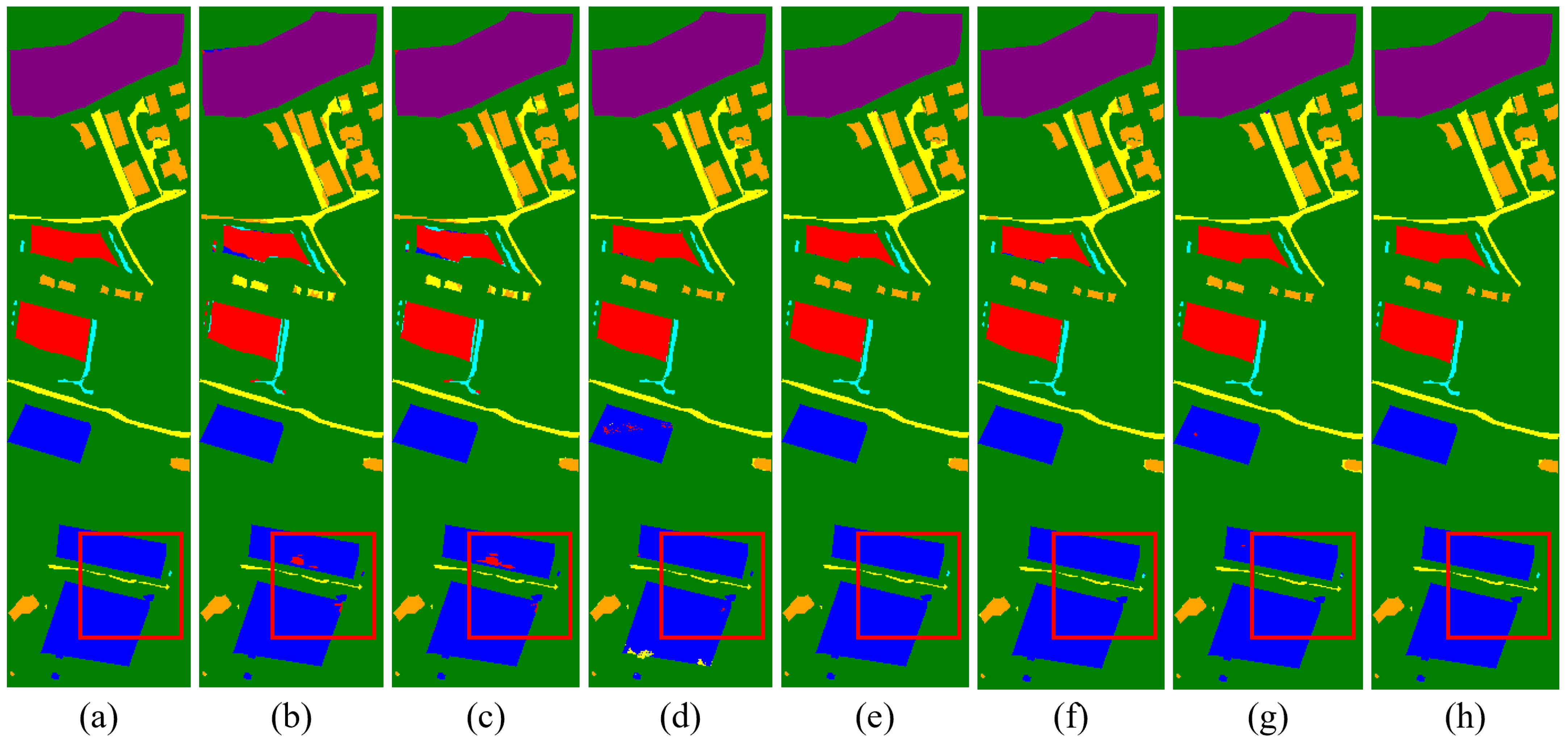
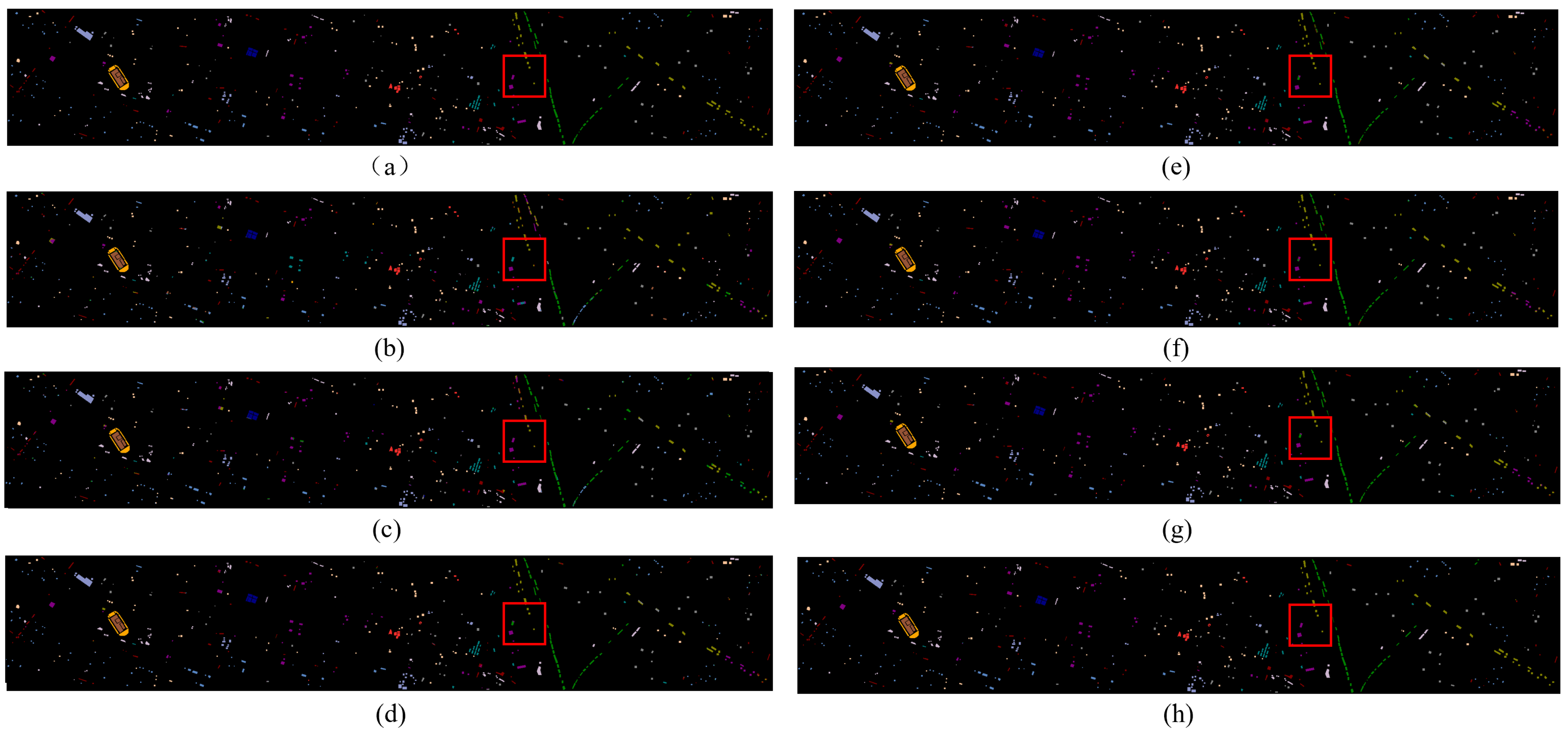
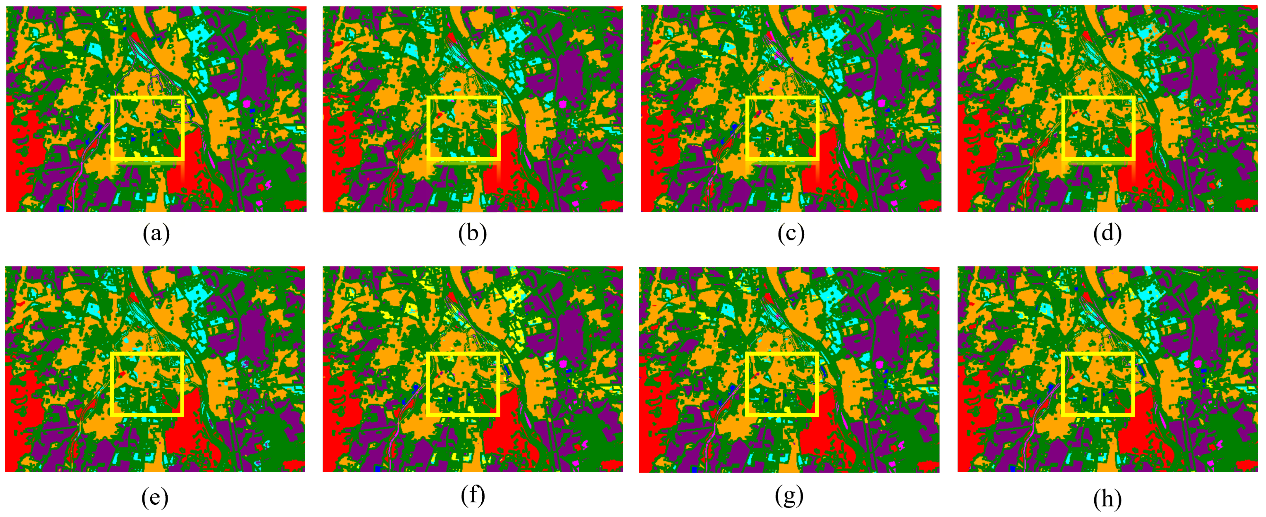
The classification outcomes for each method, which correspond to three datasets, are displayed in Figure 12, Figure 13 and Figure 14. The borders produced by our method are more distinct than those produced by other methods, further demonstrating its superior classification performance and consistency with the numerical data displayed in the table.

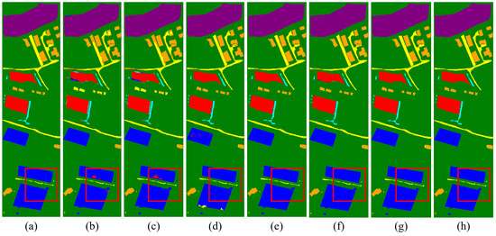
Figure 12. Classification maps by different models on the Trento dataset. (a) Ground truth map. (b) 2D-CNN (94.99%). (c) 3D-CNN (95.18%). (d) M2FNet (98.82%). (e) CALC (98.44%). (f) DSHF (98.74%). (g) Coupled CNN (98.87%). (h) Proposed (99.76%).

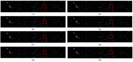
Figure 13. Classification maps by different models on the Houston dataset. (a) Ground truth map. (b) 2D-CNN (79.23%). (c) 3D-CNN (87.14%). (d) M2FNet (93.53%). (e) CALC (93.50%). (f) DSHF (91.79%). (g) Coupled CNN (95.73%). (h) Proposed (99.92%).

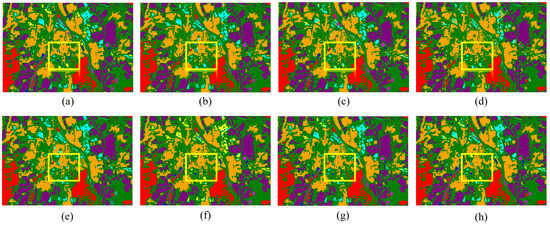
Figure 14. Classification maps by different models on the Augsburg dataset. (a) Ground truth map. (b) 2D-CNN (92.53%). (c) 3D-CNN (93.01%). (d) M2FNet (90.61%). (e) CALC (91.43%). (f) DSHF (90.21%). (g) Coupled CNN (92.13%). (h) Proposed (97.41%).

4.5. Ablation Analysis

4.5.1. Ablation Experiments on Various Fusion Methods

In order to find the most suitable fusion method for remote sensing data, we carried out a detailed study of the feature fusion module of TCPSNet and designed six combined fusion methods, as shown in Table 5. F-Sum, F-Max and F-PagFM are three feature-level fusion methods only, in which the summation, maximization and PagFM function method are used in fusion, respectively. DF-Sum, DF-Max and DF-PagFM are three fusion methods for the combination of feature level and decision level. The same represents the summation, maximization and PagFM function method. The accuracy evaluation index here is the overall accuracy, and the optimal results are shown in bold. From the experimental results, it can be seen that, among the three combinations of F-Sum, F-Max and F-PagFM using only feature-level fusion, the combination using the PagFM function tends to have higher classification accuracy. And the fusion methods of the three feature-level and decision-level combinations have a significant improvement in accuracy over the three feature-level fusion methods only; taking the PagFM function method for the Augsburg dataset as an example, the OA improves from 97.17% to 97.41% by using feature-level and decision-level fusion at the same time.

Table 5. Classification performance obtained by different fusion methods (overall accuracy (%)).

	F-Sum	F-Max	F-PagFM	DF-Sum	DF-Max	DF-PagFM
Trento	99.71	99.65	99.77	99.77	99.73	99.85
Houston	99.72	99.73	99.78	99.91	99.83	99.92
Augsburg	97.03	96.60	97.17	97.17	97.24	97.41

4.5.2. Ablation Experiments on Various Feature Extraction Modules

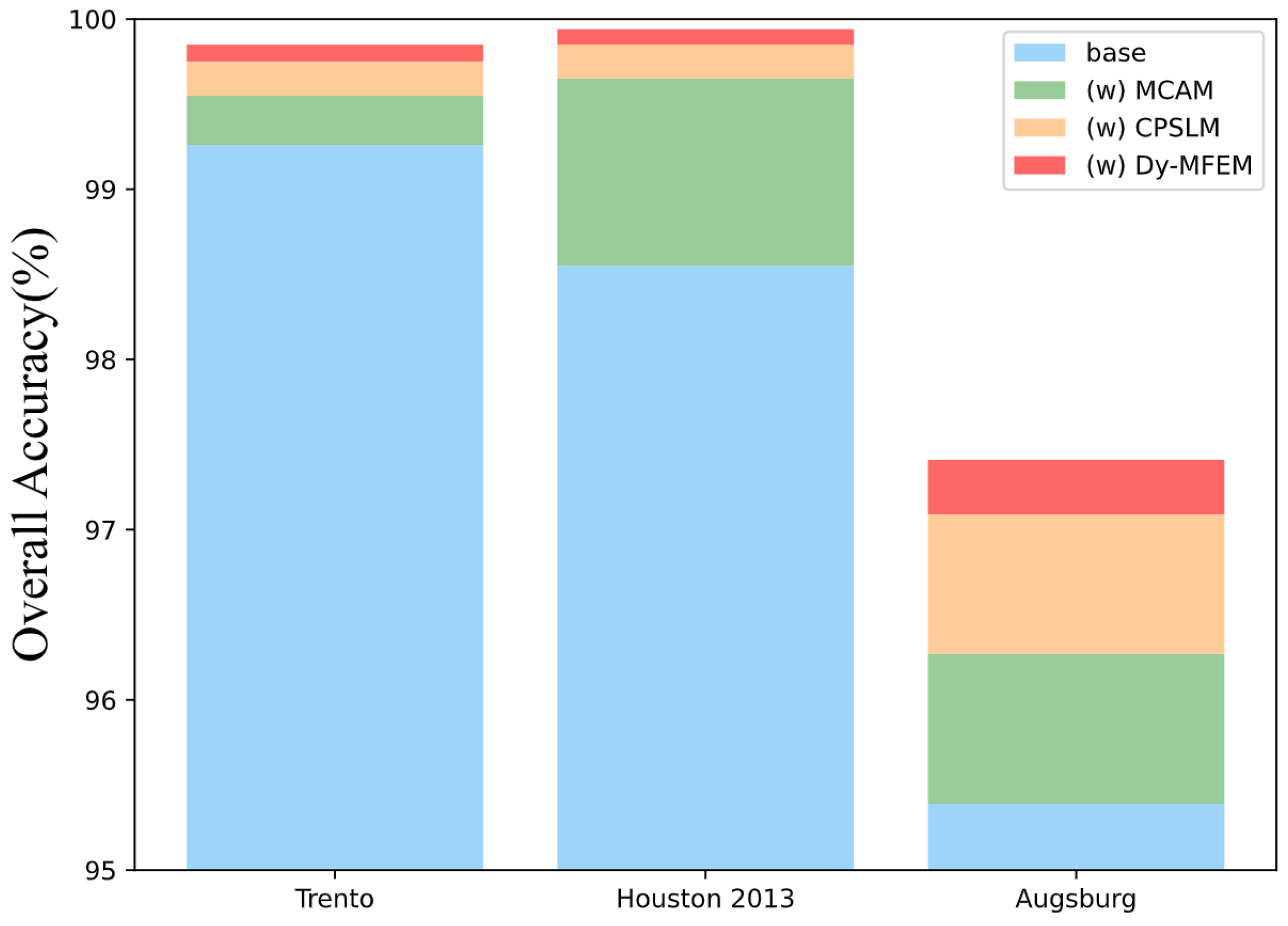
Since TCPSNet covers multiple modules, we further explore the effect of different modules on the classification ability through ablation experiments. We target the three feature extraction modules, namely MCAM, CPSLM and Dy-MFEM, and remove them to verify their effectiveness, as shown in Figure 15. The blue color indicates the classification accuracy when the three modules are removed and only part of the CNN is retained for shallow feature extraction and the fusion method proposed in this paper is used. The green, orange and red colors indicate the performance improvement after adding MCAM, CPSLM and Dy-MFEM, in which, for fairness, all fusion methods are using the DF-PagFM mentioned above, and OA is also used as the evaluation index of the classification performance. Taking the representative Trento dataset as an example, Table 6 shows the results of more detailed ablation experiments on this dataset to study the interactions and complexity between components (OA as an evaluation metric for classification performance).

Figure 15. Ablation experiments using different modules on three datasets (overall accuracy).

Table 6. Ablation analysis of different components in TCPSNet on the Trento dataset (overall accuracy (%)).

MCAM	CPSLM	Dy-MFEM	OA (%)
✓	✓	✓	99.85
✓	✓	×	99.75
×	✓	✓	99.70
✓	×	✓	99.76
✓	×	×	99.55
×	✓	×	99.69
×	×	✓	99.67
×	×	×	99.26

Based on the experimental outcomes of the three datasets, it is evident that the inclusion of the MCAM has greatly increased the accuracy. This shows that the CHA module effectively fuses the features of multimodal remote sensing data and mines the deep features of remote sensing data. But in the Trento datasets, the MCAM’s contribution is not outstanding. This may be the case because applying a Transformer encoder straight to Trento, a small dataset, will likely result in the loss of many two-dimensional image structures and a decrease in classification accuracy. However, it can also be seen that the use of CPSLM and Dy-MFEM alone without the MCAM also results in a 0.43% and 0.41% improvement in the classification results, which shows that these two modules have a good performance in some of the scenarios where the dataset is small. In the Augsburg dataset, the CPSLM’s contribution even appears to be approaching that of the MCAM. Meanwhile, if we focus on Dy-MFEM, the Houston and Trento datasets do not show significant accuracy improvement after adding this module, but for the Augsburg dataset, which is more difficult to classify, the accuracy improvement brought by Dy-MFEM is very significant. It can be seen that, in the more difficult to classify datasets, Dy-MFEM can make full use of the significant a priori knowledge on remote sensing images to mine new features and create conditions for subsequent deep feature extraction.

4.6. Sample Size Analysis

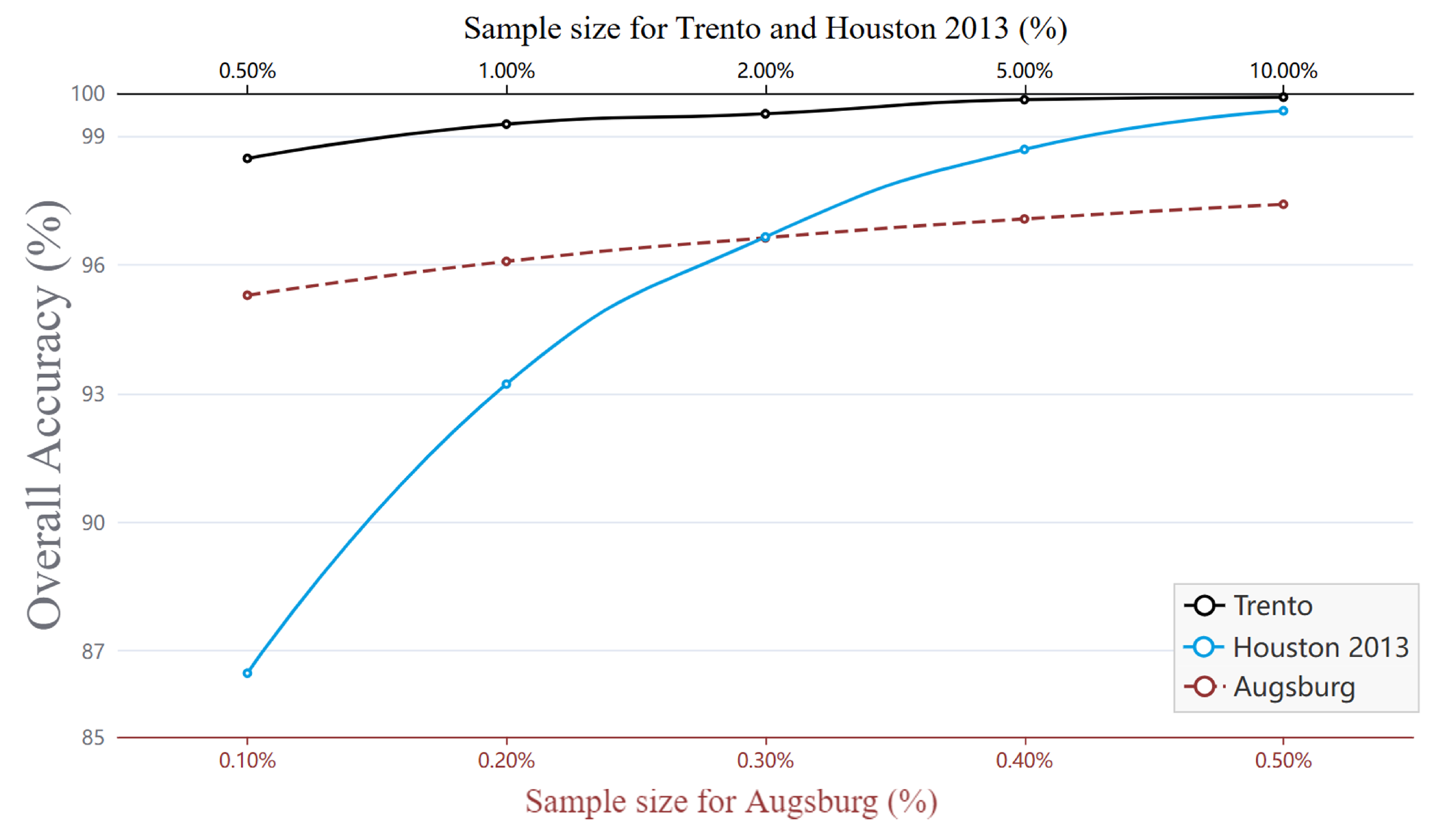
In order to test the performance of our network in scenarios such as insufficient number of sample markers and poor quality of sample markers themselves, we designed a sample size analysis experiment by re-drawing the training and test sets from the dataset in a certain proportion, where the training set extraction proportion is selected from the candidate set {0.5%, 1%, 2%, 5%, 10%}, and the remaining samples are used as the test set. Figure 16 shows the effect of different sample sizes on the overall classification accuracy of remote sensing images. It can be seen that the overall accuracy improves with the increase in the training set, but for the Trento dataset, the OA can reach 98.48% even with 0.5% of the training set samples, while for the Augsburg dataset, the OA is able to reach 95.29% even with 0.1% of the training set samples, which fully demonstrates the advantage of the method proposed in the small sample learning.

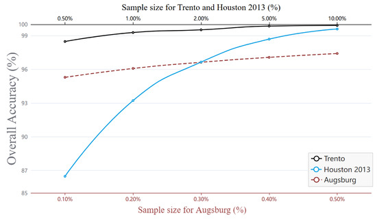
Figure 16. Influence of sample size on three datasets (overall accuracy), where the Trento and Houston datasets are represented by black and blue solid lines, with the upper axis as the horizontal axis, and the Augsburg dataset is represented by a red dashed line, with the lower axis as the horizontal axis.

4.7. Generalization Ability Analysis

We evaluate the generalizability of the network so that the method can be applied to a wider range of remote sensing data classification studies. Currently, we have created six uncommon data combinations. Specifically, these include LiDAR data combined with MSI data in the Houston 2013 dataset; HSI data combined with MSI data in the Houston 2013 dataset; SAR data combined with DSM data in the Augsburg dataset; HSI data combined with SAR data in the Augsburg dataset; HSI data combined with dual-band LiDAR data in the MUUFL dataset and HSI data combined with SAR data in the Berlin dataset.

Among them, the MUUFL dataset [42,43] was acquired in November 2010 using the reflectance optical system imaging spectrometer (ROSIS) sensor. The data consist of dual-band LiDAR data with an image size of 325 × 220 pixels and a wavelength of 1.06 $\mathsf{\mu }$m in each band. The HSI data, which cover the same area and have the same image size, consist of 72 spectral bands with spectral wavelengths covering the range of 0.38 $\mathsf{\mu }$m to 1.05 $\mathsf{\mu }$m, but due to noise, 8 bands were rejected, leaving 64 bands.

The Berlin dataset [44,45] is derived from the work of Hong et al. [3]. Its HSI data are simulated EnMAP data based on HyMap HS data and can be downloaded from the website http://doi.org/10.5880/enmap.2016.002 (accessed on 5 July 2024). In detail, the data have 244 spectral bands with a size of 797 × 220 pixels and a wavelength range of 0.4 $\mathsf{\mu }$m to 2.5 $\mathsf{\mu }$m.The SAR data in the same region are derived from the Sentinel-1 dual pol (VV-VH) single look complex (SLC) and have the same image size.

The training and test sample allocations used for MUUFL and Berlin are shown in Table 7, and the training and test sample allocations used for Houston 2013 and Augsburg are consistent with the previous experiments. Table 8 shows the experimental results for the six dataset combinations.

Table 7. Training and test sample numbers for MUUFL and Berlin datasets.

Class	MUUFL Dataset			Berlin Dataset
	Class Name	Training.	Test.	Class Name	Training.	Test.
C01	Trees	150	23,096	Forest	443	54,511
C02	Mostly Grass	150	4120	Residential Area	423	268,219
C03	Mixed Ground Surface	150	6732	Industrial Area	499	19,067
C04	Dirt and Sand	150	1676	Low Plants	376	58,906
C05	Road	150	6537	Soil	331	17,095
C06	Water	150	316	Allotment	280	13,025
C07	Buildings Shadow	150	2083	Commercial Area	298	24,526
C08	Buildings	150	6090	Water	170	6502
C09	Sidewalk	150	1235
C10	Yellow Curb	150	33
C11	Cloth Panels	150	119
-	Total	1650	52,037	Total	2820	461,851

Table 8. Classification accuracies (%) and Kappa coefficients obtained by different combination methods.

	Houston (M + L)	Houston (H + M)	Augsburg (S + L)	Augsburg (H + S)	MUUFL (H + L)	Berlin (H + S)
OA (%)	99.67	99.91	73.39	97.03	87.97	91.96
AA (%)	99.65	99.87	47.31	85.07	71.88	92.67
Kappa × 100	99.61	99.81	62.18	95.74	85.34	87.86

5. Conclusions

In this paper, a novel TCPSNet is proposed for the classification of multi-source remote sensing data. The network uses a dynamic multi-scale method for feature extraction to take advantage of the significant a priori knowledge of remote sensing data, then combines the use of the MCAM and CPSLM to obtain the modeling of deep features, and fully combines the heterogeneous features of multimodal data for interaction-induced learning, and ultimately uses a combinatorial fusion method to fuse the extracted local and global features. Our experiments on the Trento, Houston 2013, Augsburg, MUUFL and Berlin datasets show that the proposed method achieves good classification results with overall accuracies of 99.76%, 99.92%, 97.41%, 87.97% and 97.96%, respectively, while the validity of each of Dy-MFEM, MCAM, CPSLM and fusion module is demonstrated through extensive ablation experiments. Moreover, the experiments we conducted also evaluated the extent to which different hyperparameters affect the classification performance and their usability in small sample learning.

At present, our network computation efficiency is still unsatisfactory, so in the future, we will continue to explore practical ways to improve the network computation efficiency and reduce the number of parameters, in order to help the construction of smart cities.

References

- Yuan, Y.; Meng, X.; Sun, W.; Yang, G.; Wang, L.; Peng, J.; Wang, Y. Multi-Resolution Collaborative Fusion of SAR, Multispectral and Hyperspectral Images for Coastal Wetlands Mapping. Remote Sens. 2022, 14, 3492. [Google Scholar] [CrossRef]
- Zhang, M.; Zhao, X.; Li, W.; Zhang, Y.; Tao, R.; Du, Q. Cross-Scene Joint Classification of Multisource Data with Multilevel Domain Adaption Network. IEEE Trans. Neural Netw. Learn. Syst. 2023, 35, 11514–11526. [Google Scholar] [CrossRef] [PubMed]
- Hong, D.; Hu, J.; Yao, J.; Chanussot, J.; Zhu, X.X. Multimodal remote sensing benchmark datasets for land cover classification with a shared and specific feature learning model. ISPRS J. Photogramm. Remote Sens. 2021, 178, 68–80. [Google Scholar] [CrossRef] [PubMed]
- Li, X.; Wang, L.; Guan, H.; Chen, K.; Zang, Y.; Yu, Y. Urban Tree Species Classification Using UAV-Based Multispectral Images and LiDAR Point Clouds. J. Geovis. Spat. Anal. 2024, 8, 5. [Google Scholar] [CrossRef]
- Ibrahim, F.; Rasul, G.; Abdullah, H. Improving Crop Classification Accuracy with Integrated Sentinel-1 and Sentinel-2 Data: A Case Study of Barley and Wheat. J. Geovis. Spat. Anal. 2023, 7, 22. [Google Scholar] [CrossRef]
- Ge, C.; Du, Q.; Li, W.; Li, Y.; Sun, W. Hyperspectral and LiDAR Data Classification Using Kernel Collaborative Representation Based Residual Fusion. IEEE J. Sel. Top. Appl. Earth Obs. Remote Sens. 2019, 12, 1963–1973. [Google Scholar] [CrossRef]
- Benediktsson, J.; Palmason, J.; Sveinsson, J. Classification of hyperspectral data from urban areas based on extended morphological profiles. IEEE Trans. Geosci. Remote Sens. 2005, 43, 480–491. [Google Scholar] [CrossRef]
- Camps-Valls, G.; Gomez-Chova, L.; Munoz-Mari, J.; Vila-Frances, J.; Calpe-Maravilla, J. Composite kernels for hyperspectral image classification. IEEE Geosci. Remote Sens. Lett. 2006, 3, 93–97. [Google Scholar] [CrossRef]
- Rasti, B.; Ulfarsson, M.O.; Sveinsson, J.R. Hyperspectral Feature Extraction Using Total Variation Component Analysis. IEEE Trans. Geosci. Remote Sens. 2016, 54, 6976–6985. [Google Scholar] [CrossRef]
- Liao, W.; Bellens, R.; Piûrĭcă, A.; Gautama, S.; Philips, W. Combining feature fusion and decision fusion for classification of hyperspectral and LiDAR data. In Proceedings of the 2014 IEEE Geoscience and Remote Sensing Symposium, IEEE, Quebec City, QC, Canada, 13–18 July 2014; pp. 1241–1244. [Google Scholar] [CrossRef]
- Xu, J.; Xiong, Z.; Bhattacharyya, S.P. PIDNet: A Real-time Semantic Segmentation Network Inspired by PID Controllers. In Proceedings of the 2023 IEEE/CVF Conference on Computer Vision and Pattern Recognition (CVPR), Vancouver, BC, Canada, 13–18 July 2023; pp. 19529–19539. [Google Scholar] [CrossRef]
- Zhao, W.; Du, S. Spectral–spatial feature extraction for hyperspectral image classification: A dimension reduction and deep learning approach. IEEE Trans. Geosci. Remote Sens. 2016, 54, 4544–4554. [Google Scholar] [CrossRef]
- Chen, Y.; Jiang, H.; Li, C.; Jia, X.; Ghamisi, P. Deep Feature Extraction and Classification of Hyperspectral Images Based on Convolutional Neural Networks. IEEE Trans. Geosci. Remote Sens. 2016, 54, 6232–6251. [Google Scholar] [CrossRef]
- Roy, S.K.; Deria, A.; Hong, D.; Ahmad, M.; Plaza, A.; Chanussot, J. Hyperspectral and LiDAR Data Classification Using Joint CNNs and Morphological Feature Learning. IEEE Trans. Geosci. Remote Sens. 2022, 60, 5530416. [Google Scholar] [CrossRef]
- Hong, D.; Gao, L.; Hang, R.; Zhang, B.; Chanussot, J. Deep Encoder–Decoder Networks for Classification of Hyperspectral and LiDAR Data. IEEE Geosci. Remote Sens. Lett. 2022, 19, 5500205. [Google Scholar] [CrossRef]
- Du, X.; Zheng, X.; Lu, X.; Doudkin, A.A. Multisource Remote Sensing Data Classification with Graph Fusion Network. IEEE Trans. Geosci. Remote Sens. 2021, 59, 10062–10072. [Google Scholar] [CrossRef]
- Lu, T.; Ding, K.; Fu, W.; Li, S.; Guo, A. Coupled adversarial learning for fusion classification of hyperspectral and LiDAR data. Inf. Fusion 2023, 93, 118–131. [Google Scholar] [CrossRef]
- He, J.; Zhao, L.; Yang, H.; Zhang, M.; Li, W. HSI-BERT: Hyperspectral Image Classification Using the Bidirectional Encoder Representation from Transformers. IEEE Trans. Geosci. Remote Sens. 2020, 58, 165–178. [Google Scholar] [CrossRef]
- Li, Y.; Hou, Q.; Zheng, Z.; Cheng, M.M.; Yang, J.; Li, X. Large Selective Kernel Network for Remote Sensing Object Detection. In Proceedings of the 2023 IEEE/CVF International Conference on Computer Vision (ICCV), Paris, France, 1–6 October 2023; pp. 16748–16759. [Google Scholar] [CrossRef]
- Chen, Y.; Li, C.; Ghamisi, P.; Jia, X.; Gu, Y. Deep Fusion of Remote Sensing Data for Accurate Classification. IEEE Geosci. Remote Sens. Lett. 2017, 14, 1253–1257. [Google Scholar] [CrossRef]
- Xu, X.; Li, W.; Ran, Q.; Du, Q.; Gao, L.; Zhang, B. Multisource Remote Sensing Data Classification Based on Convolutional Neural Network. IEEE Trans. Geosci. Remote Sens. 2018, 56, 937–949. [Google Scholar] [CrossRef]
- Li, H.; Ghamisi, P.; Soergel, U.; Zhu, X.X. Hyperspectral and LiDAR fusion using deep three-stream convolutional neural networks. Remote Sens. 2018, 10, 1649. [Google Scholar] [CrossRef]
- Hang, R.; Li, Z.; Ghamisi, P.; Hong, D.; Xia, G.; Liu, Q. Classification of Hyperspectral and LiDAR Data Using Coupled CNNs. IEEE Trans. Geosci. Remote Sens. 2020, 58, 4939–4950. [Google Scholar] [CrossRef]
- Cao, M.; Zhao, G.; Lv, G.; Dong, A.; Guo, Y.; Dong, X. Spectral–Spatial–Language Fusion Network for Hyperspectral, LiDAR, and Text Data Classification. IEEE Trans. Geosci. Remote Sens. 2024, 62, 5503215. [Google Scholar] [CrossRef]
- Wu, X.; Hong, D.; Chanussot, J. Convolutional Neural Networks for Multimodal Remote Sensing Data Classification. IEEE Trans. Geosci. Remote Sens. 2022, 60, 5517010. [Google Scholar] [CrossRef]
- Wang, J.; Li, J.; Shi, Y.; Lai, J.; Tan, X. AM³Net: Adaptive Mutual-Learning-Based Multimodal Data Fusion Network. IEEE Trans. Circuits Syst. Video Technol. 2022, 32, 5411–5426. [Google Scholar] [CrossRef]
- Mohla, S.; Pande, S.; Banerjee, B.; Chaudhuri, S. FusAtNet: Dual Attention based SpectroSpatial Multimodal Fusion Network for Hyperspectral and LiDAR Classification. In Proceedings of the 2020 IEEE/CVF Conference on Computer Vision and Pattern Recognition Workshops (CVPRW), Seattle, WA, USA, 14–19 June 2020; pp. 416–425. [Google Scholar] [CrossRef]
- Feng, Y.; Song, L.; Wang, L.; Wang, X. DSHFNet: Dynamic Scale Hierarchical Fusion Network Based on Multiattention for Hyperspectral Image and LiDAR Data Classification. IEEE Trans. Geosci. Remote Sens. 2023, 61, 5522514. [Google Scholar] [CrossRef]
- Ren, Q.; Tu, B.; Liao, S.; Chen, S. Hyperspectral Image Classification with IFormer Network Feature Extraction. Remote Sens. 2022, 14, 4866. [Google Scholar] [CrossRef]
- Zhao, G.; Ye, Q.; Sun, L.; Wu, Z.; Pan, C.; Jeon, B. Joint Classification of Hyperspectral and LiDAR Data Using a Hierarchical CNN and Transformer. IEEE Trans. Geosci. Remote Sens. 2023, 61, 5500716. [Google Scholar] [CrossRef]
- Zhao, F.; Li, S.; Zhang, J.; Liu, H. Convolution Transformer Fusion Splicing Network for Hyperspectral Image Classification. IEEE Geosci. Remote Sens. Lett. 2023, 20, 5501005. [Google Scholar] [CrossRef]
- Sun, L.; Wang, X.; Zheng, Y.; Wu, Z.; Fu, L. Multiscale 3-D–2-D Mixed CNN and Lightweight Attention-Free Transformer for Hyperspectral and LiDAR Classification. IEEE Trans. Geosci. Remote Sens. 2024, 62, 2100116. [Google Scholar] [CrossRef]
- Roy, S.K.; Sukul, A.; Jamali, A.; Haut, J.M.; Ghamisi, P. Cross Hyperspectral and LiDAR Attention Transformer: An Extended Self-Attention for Land Use and Land Cover Classification. IEEE Trans. Geosci. Remote Sens. 2024, 62, 5512815. [Google Scholar] [CrossRef]
- Ni, K.; Wang, D.; Zheng, Z.; Wang, P. MHST: Multiscale Head Selection Transformer for Hyperspectral and LiDAR Classification. IEEE J. Sel. Top. Appl. Earth Obs. Remote Sens. 2024, 17, 5470–5483. [Google Scholar] [CrossRef]
- Wang, S.; Hou, C.; Chen, Y.; Liu, Z.; Zhang, Z.; Zhang, G. Classification of Hyperspectral and LiDAR Data Using Multi-Modal Transformer Cascaded Fusion Net. Remote Sens. 2023, 15, 4142. [Google Scholar] [CrossRef]
- Zhang, Y.; Xu, S.; Hong, D.; Gao, H.; Zhang, C.; Bi, M.; Li, C. Multimodal Transformer Network for Hyperspectral and LiDAR Classification. IEEE Trans. Geosci. Remote Sens. 2023, 61, 5514317. [Google Scholar] [CrossRef]
- Ding, K.; Lu, T.; Fu, W.; Li, S.; Ma, F. Global–Local Transformer Network for HSI and LiDAR Data Joint Classification. IEEE Trans. Geosci. Remote Sens. 2022, 60, 5541213. [Google Scholar] [CrossRef]
- Rasti, B.; Ghamisi, P.; Gloaguen, R. Hyperspectral and LiDAR Fusion Using Extinction Profiles and Total Variation Component Analysis. IEEE Trans. Geosci. Remote Sens. 2017, 55, 3997–4007. [Google Scholar] [CrossRef]
- Debes, C.; Merentitis, A.; Heremans, R.; Hahn, J.; Frangiadakis, N.; van Kasteren, T.; Liao, W.; Bellens, R.; Pižurica, A.; Gautama, S.; et al. Hyperspectral and LiDAR Data Fusion: Outcome of the 2013 GRSS Data Fusion Contest. IEEE J. Sel. Top. Appl. Earth Obs. Remote Sens. 2014, 7, 2405–2418. [Google Scholar] [CrossRef]
- Ghamisi, P.; Rasti, B.; Yokoya, N.; Wang, Q.; Hofle, B.; Bruzzone, L.; Bovolo, F.; Chi, M.; Anders, K.; Gloaguen, R.; et al. Multisource and Multitemporal Data Fusion in Remote Sensing: A Comprehensive Review of the State of the Art. IEEE Geosci. Remote Sens. Mag. 2019, 7, 6–39. [Google Scholar] [CrossRef]
- Baumgartner, A.; Gege, P.; Köhler, C.; Lenhard, K.; Schwarzmaier, T. Characterisation methods for the hyperspectral sensor HySpex at DLR’s calibration home base. In Proceedings of the Sensors, Systems, and Next-Generation Satellites XVI; Meynart, R., Neeck, S.P., Shimoda, H., Eds.; International Society for Optics and Photonics, SPIE: Bellingham, WA, USA, 2012; p. 85331H. [Google Scholar] [CrossRef]
- Gader, P.; Zare, A.; Close, R.; Aitken, J.; Tuell, G. MUUFL Gulfport Hyperspectral and LiDAR Airborne Data Set; University of Florida: Gainesville, FL, USA, 2013. [Google Scholar]
- Du, X.; Zare, A. Technical Report: Scene Label Ground Truth Map for MUUFL Gulfport Data Set; University of Florida: Gainesville, FL, USA, 2017. [Google Scholar]
- Okujeni, A.; Linden, S.V.D.; Hostert, P. Berlin-Urban-Gradient Dataset 2009: An EnMap Preparatory Flight Campaign; GFZ Data Services: Potsdam, Germany, 2016. [Google Scholar]
- Haklay, M.; Weber, P. OpenStreetMap: User-Generated Street Maps. IEEE Pervasive Comput. 2008, 7, 12–18. [Google Scholar] [CrossRef]
Disclaimer/Publisher’s Note: The statements, opinions and data contained in all publications are solely those of the individual author(s) and contributor(s) and not of MDPI and/or the editor(s). MDPI and/or the editor(s) disclaim responsibility for any injury to people or property resulting from any ideas, methods, instructions or products referred to in the content. |
© 2024 by the authors. Licensee MDPI, Basel, Switzerland. This article is an open access article distributed under the terms and conditions of the Creative Commons Attribution (CC BY) license (https://creativecommons.org/licenses/by/4.0/).