Abstract
Groundwater is crucial in mediating the interactions between the carbon and water cycles. Recently, groundwater storage depletion has been identified as a significant source of carbon dioxide (CO2) emissions. Here, we developed two data-driven models—XGBoost and convolutional neural network–long short-term memory (CNN-LSTM)—based on multi-satellite and reanalysis data to monitor CO2 emissions resulting from groundwater storage depletion in South Korea. The data-driven models developed in this study provided reasonably accurate predictions compared with in situ groundwater storage anomaly (GWSA) observations, identifying relatively high groundwater storage depletion levels in several regions over the past decade. For each administrative region exhibiting a decreasing groundwater storage trend, the corresponding CO2 emissions were quantified based on the predicted GWSA and respective bicarbonate concentrations. For 2008–2019, XGBoost and CNN-LSTM estimated CO2 emissions to be 0.216 and 0.202 MMTCO2/year, respectively. Furthermore, groundwater storage depletion vulnerability was assessed using the entropy weight method and technique for order of preference by similarity to ideal solution (TOPSIS) to identify hotspots with a heightened potential risk of CO2 emissions. Western South Korean regions were particularly classified as high or very high regions and susceptible to groundwater storage depletion-associated CO2 emissions. This study provides a foundation for developing countermeasures to mitigate accelerating groundwater storage depletion and the consequent rise in CO2 emissions.
1. Introduction
The amount of CO2 in the atmosphere continues to increase due to the combustion of fossil fuels and deforestation [1]. In an attempt to mitigate climate change on a global scale, concerted efforts are being made to reduce CO2 emissions worldwide [2]. To understand climate change clearly and enact effective policies for mitigating this phenomenon, a holistic understanding of the water and carbon cycle processes is required [3,4]. Globally, on average, water bodies emit 7700 million metric tons of CO2 (MMTCO2) annually, with streams and rivers contributing 6600 MMTCO2/year and lakes and reservoirs accounting for 1100 MMTCO2/year [5]. Therefore, monitoring changes in water use due to accelerated climate change and the attendant changes in CO2 emissions from water bodies is paramount.
Groundwater also contributes to atmospheric carbon dynamics through the interaction between the carbon and water cycles; it releases CO2 into surface waters as well as the atmosphere. The atmospheric CO2 contribution is affected by changes in the carbon flux between groundwater and the atmosphere. In recent years, increased water use, climate change-induced events such as droughts, and declining river flows have led to a greater dependence on groundwater, causing changes in carbon flux. Consequently, groundwater storage depletion has been widely observed globally [6,7,8,9,10,11]. Jasechko et al. [6] examined 1693 aquifers worldwide and found that groundwater storage declined in 36% of aquifers from 2000 to 2022. They also confirmed the acceleration of groundwater storage depletion by observing that in 30% of the 1693 aquifers, groundwater decline in the early 21st century exceeded the rate of decline in the late 20th century.
Groundwater depletion, a previously unrecognized factor, has now been reported to contribute to CO2 fluxes. There is no net change in CO2 emissions in a steady state of the groundwater aquifer system, where recharge and discharge are balanced [12]. However, if groundwater storage is depleted at a rate exceeding its recharge, CO2 is released into the atmosphere [13,14]. Consequently, the increasing trend of groundwater depletion due to groundwater extraction, driven by factors such as climate change and drought, is likely to result in higher CO2 emissions. Wood and Hyndman [12] reported that groundwater depletion was responsible for the release of approximately 1.7 MMTCO2/year into the atmosphere in the United States during 2000–2008, and it has been ranked among the top 20 sources of carbon emissions as documented by the US Environmental Protection Agency [15]. Mishra et al. [16] investigated CO2 emissions due to groundwater depletion and pumping in India using groundwater observation wells and the Gravity Recovery and Climate Change Experiment (GRACE) satellite. They estimated that during 2002–2016, the total groundwater depletion was 122–199 billion m3, and the corresponding annual CO2 emission was approximately 0.72 MMTCO2/year in India. Based on these findings, they emphasized the importance of understanding the relationship between groundwater and carbon emissions in preventing adverse environmental impacts.
However, analyzing the spatiotemporal relationships between carbon flux and groundwater storage is challenging due to the sparsity of observational data, discontinuities in data provision periods, and the low spatial resolution of available satellite data [11]. Groundwater storage observations, which often rely on point-based measurements, may not be sufficient for capturing groundwater storage depletion associated with spatiotemporal variations in CO2 emissions. As an alternative, combining satellite data with advanced data-driven models, such as machine and deep learning models, has recently garnered interest. This approach can provide a clearer idea of groundwater storage at different temporal and spatial scales, thereby overcoming the limitations of existing satellite data. For example, data-driven models have been used to predict temporal changes in groundwater storage [17,18,19], groundwater potential [20,21,22], and groundwater drought [23,24,25], as well as for the downscaling of groundwater storage data [26,27,28]. The existing studies predominantly employed data-driven models that relied on single meteorological variables, such as precipitation or temperature, or a restricted set of input parameters. However, groundwater dynamics are influenced by a complex interplay of multiple factors, necessitating a more comprehensive and diverse set of input variables. In this study, we developed a data-driven model to predict groundwater storage anomalies (GWSAs) and depletion by integrating an extensive range of input variables, encompassing satellite-based meteorological, hydrological, and vegetation data. CO2 emissions resulting from groundwater storage depletion can be estimated more accurately by utilizing a combination of data-driven models and multi-satellite data to predict spatiotemporal variations in groundwater storage.
With projections indicating a significant future decline in groundwater storage, recognizing the vulnerability to such depletion and identifying high-risk areas become imperative, especially considering the potential for associated CO2 emissions. In this regard, vulnerability assessment has emerged as a crucial tool in water resource management [29]. While the definition of vulnerability varies, it fundamentally refers to the degree of susceptibility or inability to cope with damages and negative impacts from climate change or human activities [30]. Adger [31] further defines vulnerability as the state of being susceptible to harm due to exposure to stresses associated with environmental and social change, coupled with a lack of adaptive capacity. Therefore, this study assessed vulnerability to groundwater storage depletion using the entropy weight and technique for order of preference by similarity to ideal solution (TOPSIS) methods, which considers spatial and temporal factors, including both natural and anthropogenic impacts. In addition, potential hotspots were identified by analyzing regions susceptible to groundwater storage depletion using vulnerability assessment and associated CO2 emissions based on data-driven models. Vulnerability assessment using this technique enables the identification of areas at risk of increased CO2 emissions due to groundwater storage depletion.
In this study, we investigated the impacts and vulnerabilities of groundwater storage depletion on CO2 emissions in South Korea using machine and deep learning models based on multi-satellite data. The specific objectives were as follows: (1) to predict the GWSA based on hydrological factors using multi-satellite and reanalysis data and to validate the spatiotemporal GWSA prediction and distribution by comparing them with in situ groundwater observations; (2) to quantify the contribution of groundwater depletion to CO2 emissions using the predicted GWSA; and (3) to investigate the extent of vulnerability to groundwater storage depletion that may result in CO2 emission changes using the entropy weight method and TOPSIS.
2. Study Area and Data
2.1. Study Area
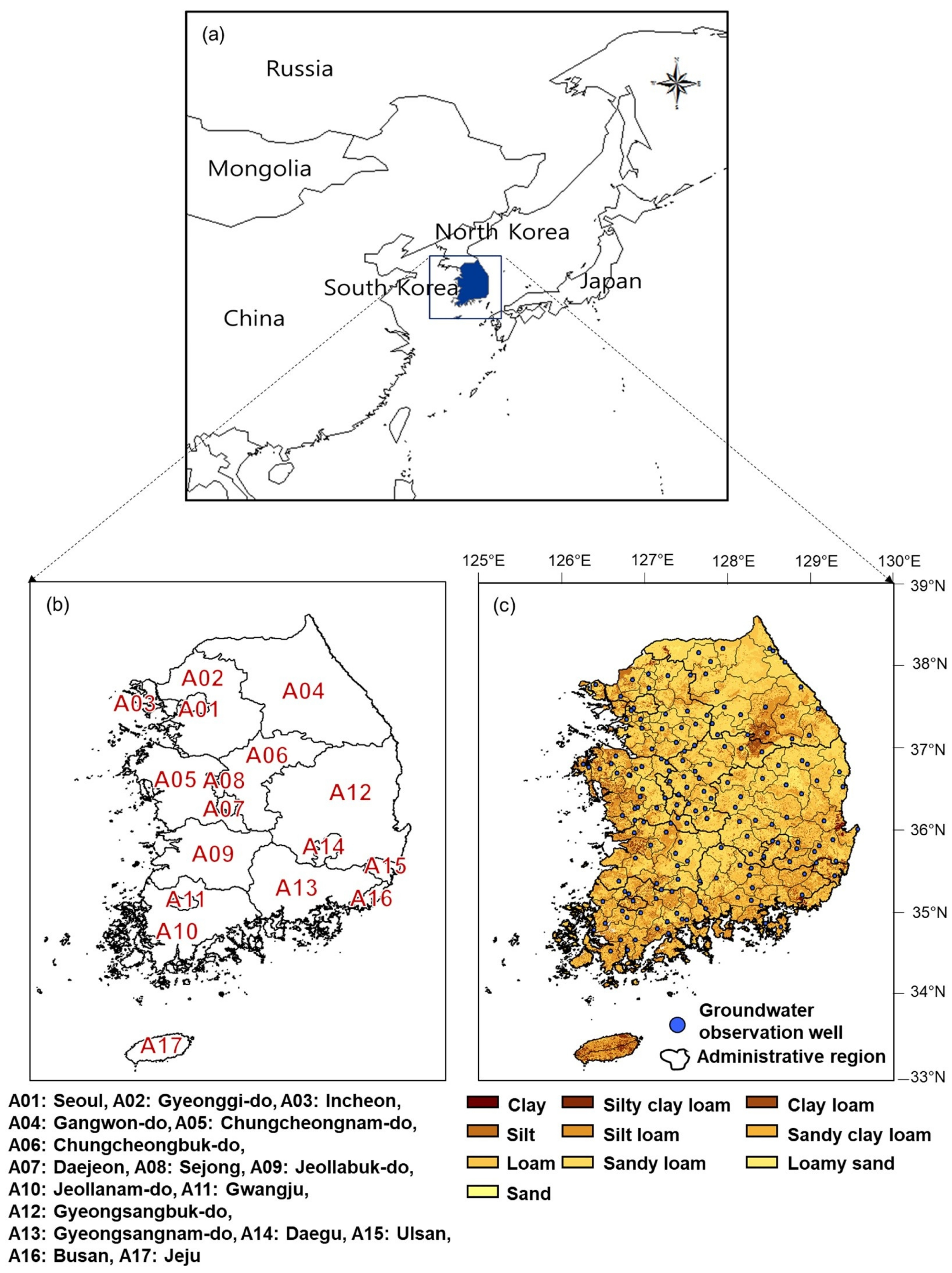
South Korea is located in East Asia (33°N to 39°N and 125°E to 130°E; Figure 1a) and is characterized by a temperate climate with a mean annual temperature of 12–14 °C and four distinct seasons. It is predominantly influenced by East Asian monsoons and typhoons. The mean annual precipitation is 1000–1800 mm, and rainfall occurs mainly during the Changma season (from July to August). South Korea consists of 160 administrative regions in 17 provinces (A01, Seoul; A02, Gyeonggi-do; A03, Incheon; A04, Gangwon-do; A05, Chungcheongnam-do; A06, Chungcheongbuk-do; A07, Daejeon; A08, Sejong; A09, Jeollabuk-do; A10, Jeollanam-do; A11, Gwangju; A12, Gyeongsangbuk-do; A13, Gyeongsangnam-do; A14, Daegu; A15, Ulsan; A16, Busan; A17, Jeju; Figure 1b). The Jeju Island region (A17) was excluded from the study area. Monthly groundwater-level data (2003–2019) from 166 stations (blue dots in Figure 1c) of the National Groundwater Monitoring Network (NGMN) were used. In addition, soil texture classification data (Figure 1c), based on a detailed soil map (1:25,000) of the National Institute of Agricultural Sciences and Korean Rural Development Administration, were used to calculate the specific yield (Sy) and convert groundwater-level data to groundwater storage. The proportions of clay (0.23%), silty clay loam (4.08%), clay loam (2.85%), silt (0.21%), silt loam (21.15%), sandy clay loam (0.59%), loam (27.61%), sandy loam (39.92%), loamy sand (3.06%), and sand (0.29%) in the soil were noted. Sandy loam, loam, and silt loam dominate the soil texture in South Korea (~89%). South Korea has a diverse geological landscape, which contributes to various types of aquifers, including alluvial, fractured rock, and volcanic aquifers. Alluvial aquifers are found in river valleys and coastal regions and are composed of unconsolidated sediments like sand, gravel, and silt, which have high porosity and permeability, making them significant sources of groundwater. In mountainous and hilly regions, fractured rock aquifers are prevalent. Jeju Island is known for its volcanic aquifers formed in basaltic rock.
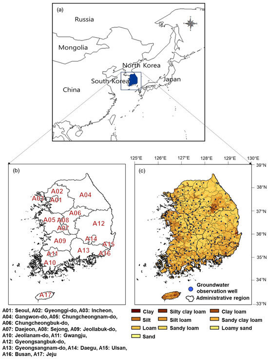
Figure 1.
Study area: (a) Locations of South Korea. (b) Provinces of South Korea. (c) Soil texture classification and groundwater observation wells.
2.2. Data
In this study, the input datasets of data-driven models consisted of the precipitation (P), mean temperature (T), soil moisture content (SM), normalized difference vegetation index (NDVI), modified normalized difference water index (MNDWI), and terrestrial water storage anomaly (TWSA) data, which were used to predict GWSA (Table 1).

Table 1.
Information on the satellite and reanalysis data.
The P data were obtained from the TMPA3B43V7 dataset produced by the Tropical Rainfall Measuring Mission (TRMM) satellite, which has been widely applied and validated in this study area [32,33]. Monthly P datasets from 2003 to 2019 with a spatial resolution of 0.25° were used. The T and SM values used in this study were provided by the global land data assimilation system (GLDAS, [34]). Monthly T and SM datasets (Noah025_M) from 2003 to 2019 with a spatial resolution of 0.25° were used.
The NDVI and MNDWI values were sourced from datasets provided by Landsat 5 (TM) and 8 (OLI) satellites. A fast line-of-sight atmospheric analysis using the spectral hypercube algorithm was performed for radiometric and atmospheric correction [35]. A total of 2652 processed images were mosaicked via nearest-neighbor sampling. The 30 m NDVI and MNDWI values over the entire period (2003–2019) were resampled to 0.25° grids.
TWSA data were determined using the equivalent water thickness converted from mass change observations provided by the GRACE satellite [36]. The GRACE data were processed at the Center for Space Research (CSR), Jet Propulsion Laboratory, and German Research Centre for Geosciences. In this study, we used the monthly TWSA data from the CSR mascon solution (release 6) at a resolution of 0.25° [37,38]. The CSR mascon data were improved upon through the measurement noise of traditional spherical harmonic coefficients through coefficient (C20, C30) replacement and filtering, thereby reducing leakage errors between coastal and land masks. Wang et al. [39] assessed the CSR mascon data, finding it to exhibit the lowest uncertainty among the available GRACE mascon solutions. GRACE data have been extensively applied and compared with in situ measurements in various studies in South Korea, demonstrating its reliability and validity [18,24,33,40]. Cubic spline interpolation was employed to fill in the monthly data gaps caused by battery issues and the 11-month hiatus between the GRACE and GRACE-FO products from July 2017 to May 2018. Cubic splines have been widely used in numerous studies due to their relative simplicity and effectiveness in gap-filling between GRACE and GRACE-FO [18,41,42,43,44].
The in situ GWSA represents the deviation for a specific month relative to the baseline average from January 2004 to December 2009. The monthly changes in groundwater-level data from 166 stations (blue dots in Figure 1c) were converted to GWSA values in terms of equivalent height by multiplying Sy by groundwater-level changes. The median Sy value for each 0.25° grid was calculated using soil texture information (Figure 1c), as reported by [45,46].
3. Methods
3.1. Prediction of GWSA
3.1.1. Machine and Deep Learning Models
Groundwater in situ data are limited in its spatial representation as it consists of point data. Although South Korea has 166 groundwater observation stations, the data are insufficient to calculate GWSA by administrative region. Consequently, satellite data present challenges for nowcasting and forecasting due to latency in data provision by institutions such as NASA. This study aims to develop data-driven models that consider the lag time of satellite and reanalysis data to predict accurate spatiotemporal GWSA.
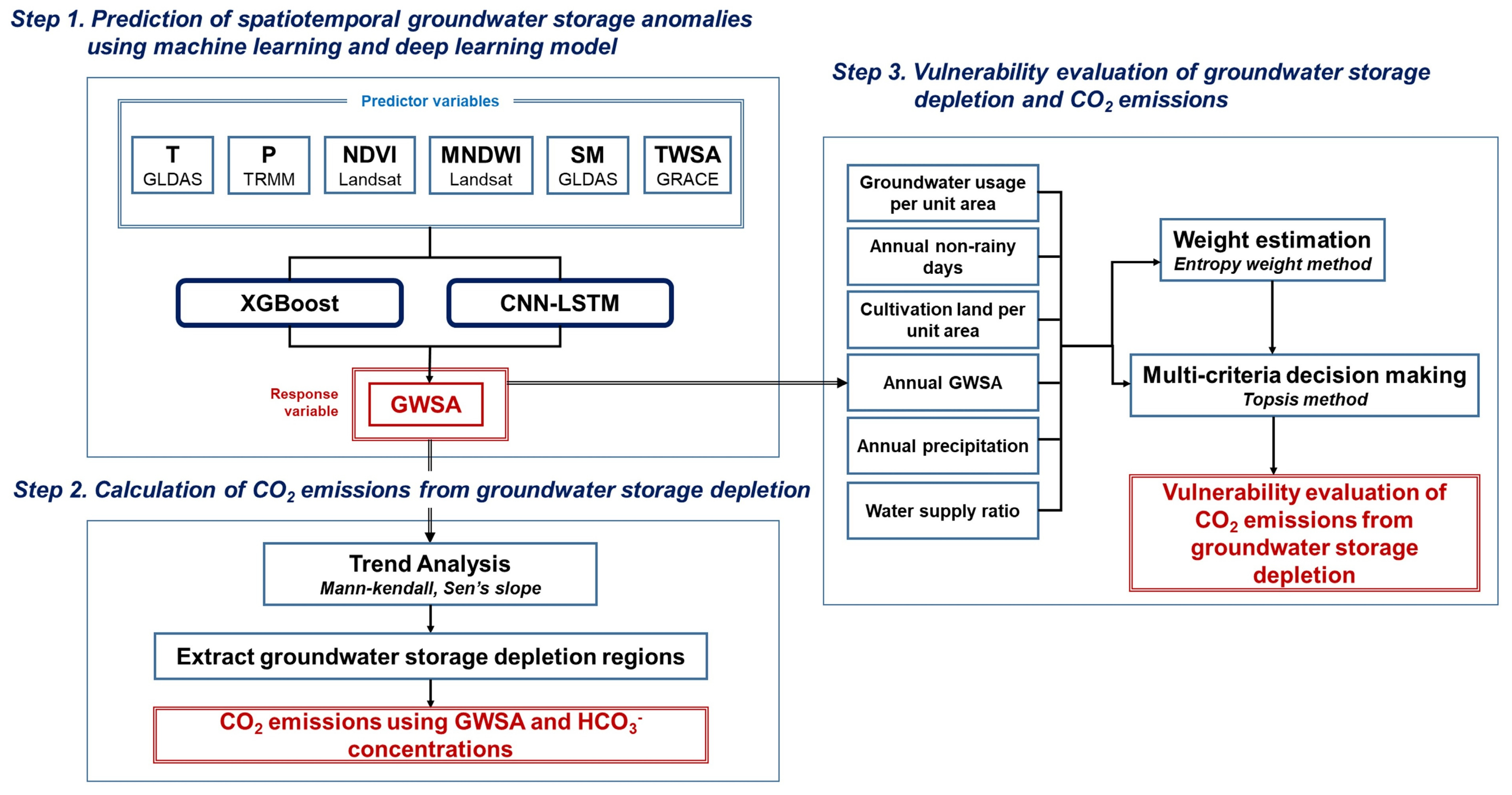
In this study, machine (XGBoost) and deep learning (convolutional neural network–long short-term memory; CNN-LSTM) models were developed to predict GWSA (Step 1 in Figure 2).
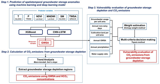
Figure 2.
A flow chart of the methodology used in this study.
XGBoost is a machine learning model that makes up for the shortcomings of the gradient boost model using residuals, which reduce errors by weighting data. It adds an overfitting prevention technique to gradient tree boosting, which is a supervised learning algorithm that sequentially combines gradient-boosting models. XGBoost is a highly accurate algorithm for regression problems (i.e., time series prediction) because it uses parallel computation to learn faster and prune unnecessary subtrees to reduce overfitting and achieve greater generalizability [47]. The CNN-LSTM model is powerful for time series prediction due to its ability to extract and learn both spatial and temporal features, leading to more accurate and reliable predictions [48].
The input variable sets for the data-driven models included satellite and reanalysis data from m months prior (t-m), specifically P(t-m), T(t-m), SM(t-m), NDVI(t-m), MNDWI(t-m), and TWSA(t-m) (Table 1 and Figure 3). The GWSA(t) is the output variable (prediction values) and was validated with in situ data (actual values) from 166 groundwater observation wells. The total period (2003–2019) of the dataset was divided into training (80%) and test (20%) periods.
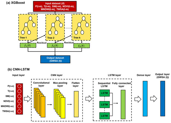
Figure 3.
Structure of data-driven models: (a) XGBoost, (b) CNN-LSTM.
The models were implemented using the XGBoost and Keras libraries in Python (version 3.6). The input variables were standardized using the min–max scaling method, which scales the data to have values between 0 and 1 to prevent overfitting in this study. The XGBoost structure consists of weak decision trees and each tree focuses on reducing the residuals (errors between the actual and predicted values) from the previous iteration to create strong learners (Figure 3a). The loss function was selected as the root mean square error (RMSE) to optimize errors in the training process in this study.
The CNN-LSTM structure consists of CNN, LSTM, and dense layers (Figure 3b). The convolutional layer extracts spatial features through an activation function (the ReLU function was used) after performing a convolutional product operation on the input data. Subsequently, the max pooling layer reduces the size of the detected feature data. Thereafter, the LSTM layer performs a time series prediction by extracting temporal features [18]. The RMSE was used as a loss function for updating the network as with the Adam optimizer in this study.
3.1.2. Hyperparameter Tuning
Hyperparameters are values that are often set by the user of an algorithm based on experience. The optimal value is not predefined and must be determined through multiple iterations. Determining optimal hyperparameter values is essential for the model to achieve high performance. Three main methods are used for tuning hyperparameters: grid search, random search, and Bayesian optimization. In this study, we used Bayesian optimization, which can handle high hyperparameter counts and large search spaces. Such methods are more efficient than grid or random search methods because they balance the exploitation and utilization of the search space [49].
Table 2 lists the hyperparameter settings used to tune the XGBoost and CNN-LSTM models and the ranges for each hyperparameter. The parameters to be optimized for XGBoost comprise tree-specific hyperparameters (number of estimators, maximum depth, minimum child depth, subsample, and colsample_bytree), which control the overall behavior and learning process of the model, and learning task-specific hyperparameters (gamma, lambda, alpha, and learning rate). In the case of CNN-LSTM, hyperparameters related to the network structure (number of filters and hidden layers, hidden units, and dropout) and those used for learning (learning rate, epochs, and iteration) were optimized. The loss function was mean square error. For both models, the time lags of 1–12 months were set for predicting the GWSA time series.
Table 2.
Hyperparameter tuning ranges for XGBoost and CNN-LSTM models.
3.2. Quantification of CO2 Emission Due to Groundwater Storage Depletion
3.2.1. Trend Analysis of Model-Predicted GWSA
In this study, the Mann–Kendall test and Sen’s slope were used to identify regions suffering groundwater storage depletion (Step 2 in Figure 2). The Mann–Kendall test is a nonparametric statistical technique that determines a trend within a certain confidence level [50], and Sen’s slope represents the slope of a linear trend [51]. As these methods are largely unaffected by missing data or outliers, they are useful for analyzing time series trends [52,53]. For each administrative region, areas with groundwater storage depletion were identified as those for which the Mann–Kendall test and Sen’s slope (p < 0.05) highlighted a decreasing trend in the GWSA predicted by the XGBoost and CNN-LSTM models.
3.2.2. CO2 Emission from Groundwater Storage Depletion
Wood and Hyndman [12] suggested that groundwater contributes to CO2 emissions through the following processes: a groundwater recharge from precipitation, reaction of recharged groundwater in aquifers, and re-exposure of groundwater to the atmosphere. Thus, CO2 emissions can be estimated by groundwater storage depletion according to groundwater use or flow to rivers and oceans and the equivalent CO2 concentration in groundwater. During the process of groundwater recharge from precipitation, water and carbon dioxide react when water enters the unsaturated zone. As water passes this zone, reacts with according to Equation (1), producing and bicarbonate () ions. Most aquifers contain gravel, sand, clay, and calcite (), which react with the produced ions to generate and ions (Equation (2)). When groundwater is extracted by pumping or discharged into rivers or the ocean, it becomes exposed to the atmosphere, causing CO2 to be released and to precipitate, as described in Equation (3). Based on a conservative assumption, half of the concentration in groundwater is converted to CO2 through the hydrological cycle [12,16]. Therefore, the concentration in groundwater plays an important role in CO2 emissions due to groundwater storage depletion. Equation (4) was used in this study to convert the (mg/L) concentration in groundwater to the equivalent CO2 concentration (; mg/L). The concentration was obtained from the NGMN and converted to the equivalent CO2 concentration for each administrative region. Subsequently, atmospheric MMTCO2/year) due to groundwater storage depletion () was estimated by Equation (5) based on groundwater storage depletion (km3/year) and equivalent CO2 concentration (kg/m3) [12,16].
3.3. Determining Groundwater Storage Depletion and CO2 Emission Vulnerability Using Entropy Weight and TOPSIS Method
Quantitative vulnerability assessment methods are often based on multi-criteria decision-making (MCDM), which involves selecting the most important or best alternative among several potential criteria. In particular, TOPSIS [54], an MCDM technique integrated with a geographic information system framework, has been widely utilized in vulnerability assessment as a rational and relatively simple computational method for deriving rankings by calculating the distances between positive and negative ideal solutions. TOPSIS is used for assessing vulnerability to various environmental phenomena, such as droughts [55,56], floods [57,58], and heat waves [59,60]. Determining the weights for the indicators is the most important factor in TOPSIS. Research is being conducted on the entropy–TOPSIS method, which combines TOPSIS with the entropy weight method [61,62] and can calculate weights objectively.
3.3.1. Selection of Indicators
The proposed methodology for quantifying CO2 emissions resulting from groundwater storage depletion is based on the premise that groundwater storage exhibits a decreasing trend. Thus, an examination of vulnerability to groundwater storage depletion can reveal areas with a potentially high risk of CO2 emissions. In this study, we employed the entropy–TOPSIS method to assess vulnerability to groundwater storage depletion. This method provides a comprehensive assessment by considering multiple factors simultaneously. Additionally, it enables an easy comparison of vulnerability across regions of interest, facilitating the identification of areas at a heightened risk.
We selected three indicators that have a positive effect on vulnerability to groundwater storage depletion: the groundwater use per unit area, number of annual non-rainy days, and cultivation land per unit area. We also selected three indicators that have a negative effect: annual GWSA (predicted by XGBoost and CNN-LSTM), precipitation, and the water supply ratio (Step 3 in Figure 2; Table 3). An increase in groundwater use per unit area has a direct impact on the depletion in groundwater storage. Consequently, as groundwater usage intensifies, the vulnerability of the area to groundwater storage depletion correspondingly increases.
Table 3.
Vulnerability assessment indicators for groundwater storage depletion.
Annual non-rainy days were selected based on the assumption that an increase in the number of non-rainy days reduces the extent of recharge, thereby reducing groundwater storage. Cultivation land per unit area was selected considering that an increase in cultivation land is expected to concurrently increase the amount of groundwater used for irrigation.
A negative GWSA indicates lower groundwater storage compared with the average (from 2004 to 2009), which is considered to increase vulnerability. A reduction in annual precipitation can lead to drought conditions, resulting in increased groundwater use due to reduced surface water availability; moreover, annual precipitation directly affects groundwater recharge rates. Hence, a lower annual precipitation is considered to increase the risk of groundwater storage depletion. Finally, if the water supply ratio in a region decreases, more people in that region will use groundwater, which is considered to increase vulnerability to groundwater storage depletion.
3.3.2. Determining Weights Using Entropy Weight Method
Calculating appropriate weights is necessary for determining the importance of indicators for vulnerability assessment. Representative methods include the equal weight, Delphi, and analytical hierarchy process methods; however, these methods rely on the subjective judgment of the researcher. Hence, we used the entropy weight method in this study, which is a simple and objective process for calculating the weights of the selected indicators. This method determines the weight according to the variance of each indicator; the more agglomerated the indicator values, the larger the weight ([61,62]; Figure 4).
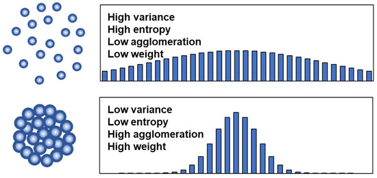
Figure 4.
Concept of entropy weight.
To calculate the entropy weight, the indicators must be standardized because they might have different units. In this study, we used the min–max method to scale the indicators to values between 0 and 1. Equation (6) represents the conversion processes for the indicators with positive or negative effects on vulnerability:
where and denote the scaled and original values of indicators, respectively.
A representative matrix can be constructed based on the standardized indicator values, as expressed in Equation (7), where is the number of indicators and is the number of regions to be analyzed.
The indicator values in the constructed matrix are used to establish a standardized index ().
Subsequently, the entropy () is calculated for each indicator, as shown below:
where denotes a constant representing the number of regions.
A scale representing the diversity of the indicators is calculated using Equation (10), and the weight can be obtained using Equation (11).
3.3.3. TOPSIS
TOPSIS considers multiple criteria simultaneously and selects the best alternative for a given purpose, based on the distance between the positive and negative ideal solutions [63].
The TOPSIS decision-making process is as follows. First, given a representative matrix (Equation (6)), each scaled indicator () is assigned a weight () determined using the entropy weight method (Equation (12)).
Second, the positive () and negative ideal solutions () for each indicator (Equations (13a,b)) for the weighted scaled values () can be calculated from the maximum and minimum values of each indicator:
where and are associated with an indicator, with having a positive and negative effect, respectively.
Third, the distance of the weighted scaled indicator value from the corresponding positive and negative ideal solution ( and ) is calculated (Equations (14a,b)). After the aforementioned steps were completed in this study, the relative closeness coefficient () was calculated for each administrative region (Equation (15)). The vulnerability of each administrative region to groundwater depletion was ranked based on the order of magnitude of the relative closeness coefficient.
4. Results
4.1. Model Performance in GWSA Prediction
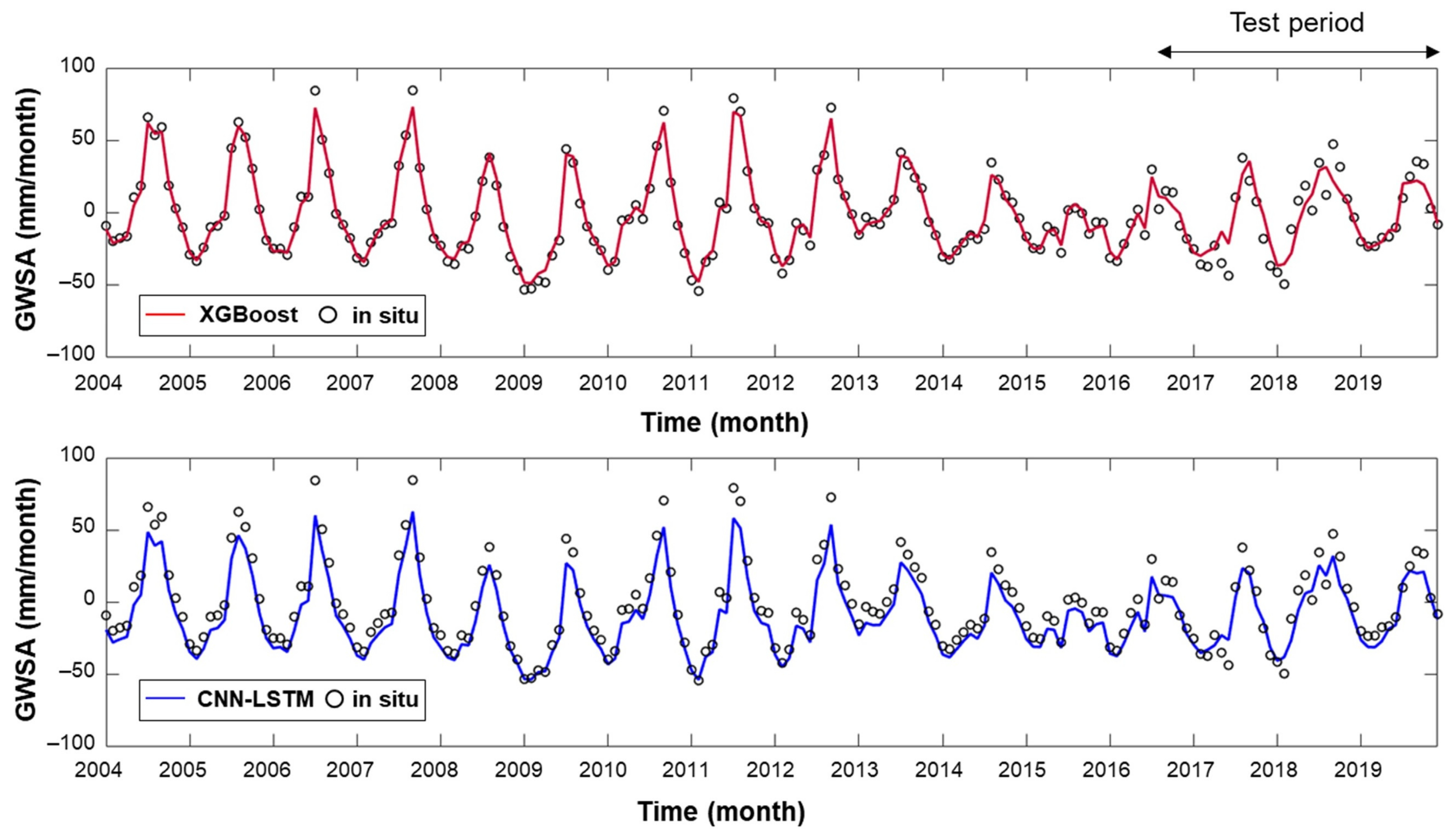
Table 4 summarizes the optimal hyperparameter values to minimize error through Bayesian optimization. Figure 5 shows the GWSA time series predicted by the XGBoost and CNN-LSTM models using optimal hyperparameters overlaid on the in situ GWSA observed in South Korea. Due to the 1–12-month lag time, the GWSA predictions span from January 2004 to December 2019. As observed in the figure, the predictions for both models match all the in situ observations, indicating that the models accurately captured the seasonality of the in situ data.
Table 4.
Optimal hyperparameter values for XGBoost and CNN-LSTM models.

Figure 5.
Model predictions of groundwater storage anomalies (GWSAs) along with in situ observations.
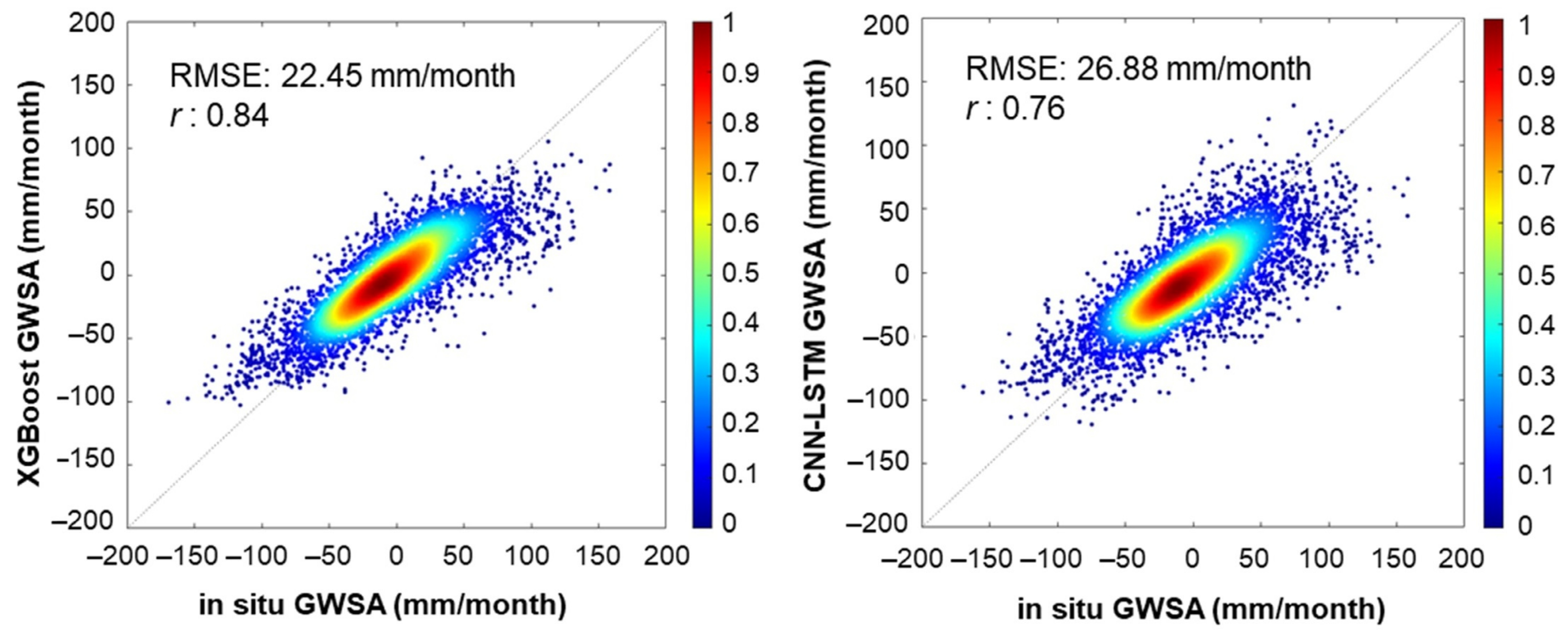
Figure 6 presents scatterplots depicting the correlation between the model-based predictions and the in situ GWSA for the test period (August 2016–December 2019). The correlation coefficients (r) were 0.84 and 0.76 for XGBoost vs. in situ and CNN-LSTM vs. in situ, respectively. The RMSE values with respect to the in situ observations were 22.45 and 26.88 mm/month for XGBoost and CNN-LSTM, respectively. Thus, the XGBoost model outperformed the CNN-LSTM model (in terms of RMSE and r) for the test period.

Figure 6.
Density scatterplots comparing predictions of XGBoost and CNN-LSTM with in situ groundwater storage anomaly (GWSA) observations during the test period.
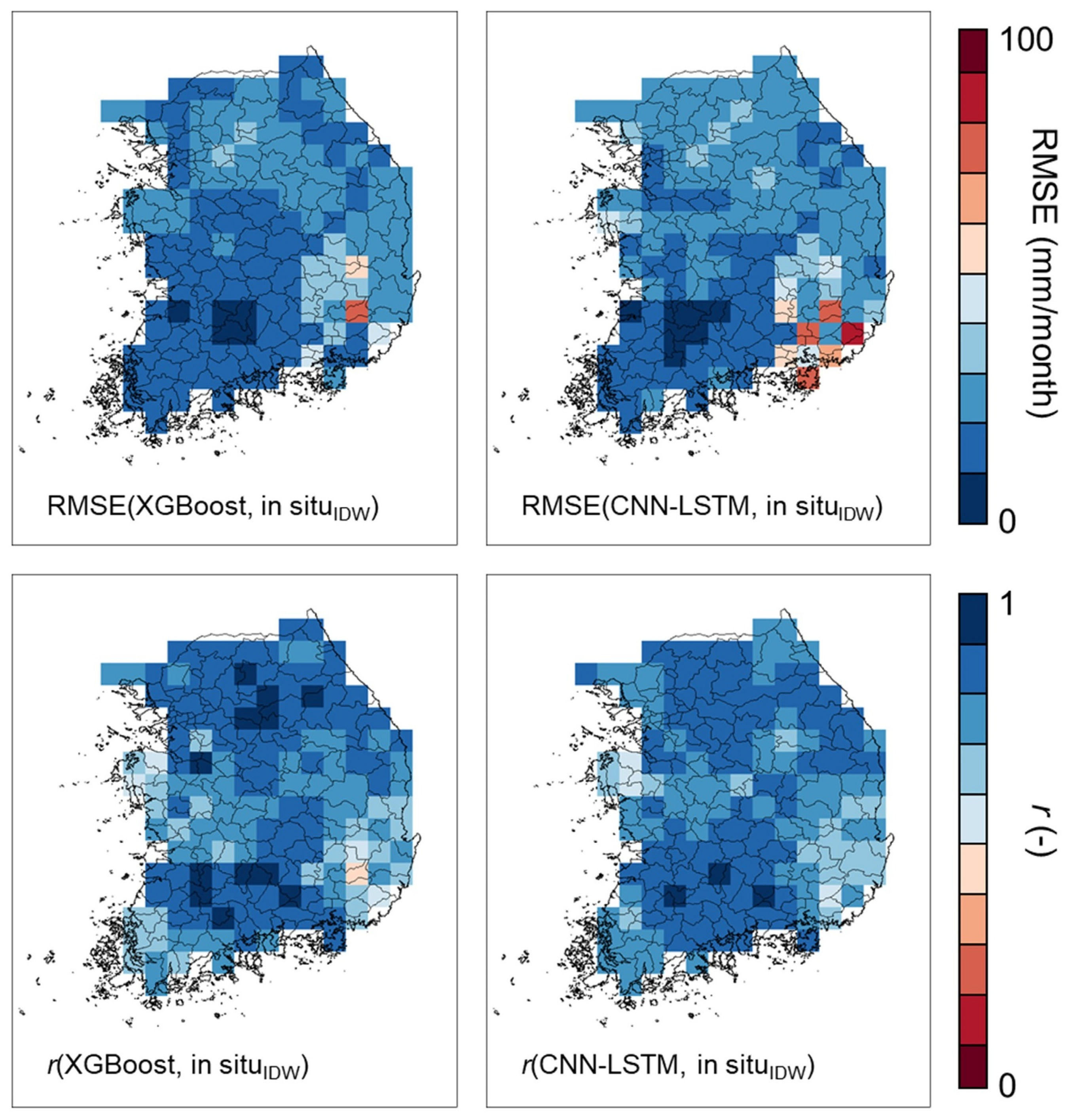
Figure 7 shows the spatial distribution maps of the RMSE and r values between the model results and in situ GWSA distributions using inverse distance weighting during the test period. The red grids indicate large errors and non-significant correlations, whereas the blue grids represent significant correlations and small errors.

Figure 7.
Spatial distribution of root mean square error (RMSE) and correlation coefficient (r) for XGBoost and CNN-LSTM predictions vs. in situ groundwater storage anomalies (GWSA) using inverse distance weighting (IDW).
4.2. Estimation of CO2 Emission Due to Groundwater Storage Depletion
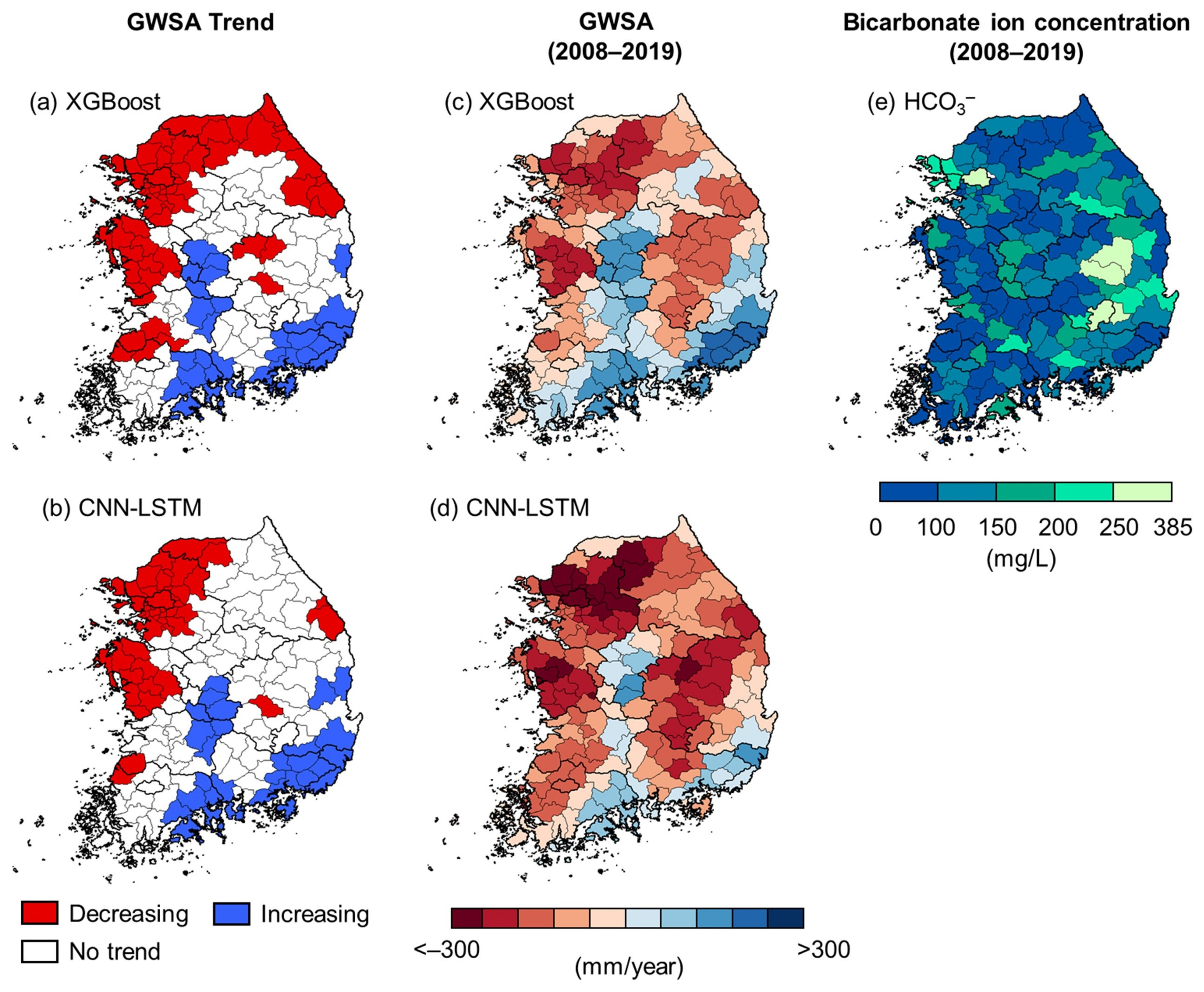
Trend analyses were conducted to identify regions with significant groundwater storage depletion and estimate the resulting CO2 emissions. Figure 8a,b show the spatial distributions of the trends determined using the Mann–Kendall test and Sen’s slope. As seen in Figure 8a, the XGBoost-predicted GWSA exhibited a significant decreasing trend (p < 0.05) in the northern (A01, A02, A03, and A04 provinces in Figure 1b) and western (A05, A09, and A10 provinces in Figure 1b) regions, accounting for 32.0% of the total area; the GWSA values were also correspondingly low in these regions during 2008–2019, as observed in Figure 8c. Additionally, the CNN-LSTM-predicted GWSA exhibited a significant decreasing trend (p < 0.05) in 16.2% of the total area, similar to that of the XGBoost-predicted GWSA, except for a few A04 provinces. Separately, significant upward trends (p < 0.05) were observed for both the XGBoost- and CNN-LSTM-predicted GWSA in the southern and central regions (Figure 8a,b), which similarly concurred with the corresponding increase in GWSA in these regions during 2008–2019 (Figure 8c,d). The overall spatial distributions of the GWSA predicted by XGBoost and CNN-LSTM were similar. However, the magnitudes of the GWSA predictions from CNN-LSTM were lower than those from XGBoost.

Figure 8.
Groundwater storage anomaly (GWSA) trend of (a) XGBoost and (b) CNN-LSTM. Median GWSA of (c) XGBoost and (d) CNN-LSTM. (e) Bicarbonate concentration.
The bicarbonate concentration was obtained from major anion analysis data of NGMN (Figure 8e; https://gims.go.kr, accessed on 20 November 2023). The median bicarbonate concentration in South Korea (~120 mg/L) is lower than that observed in the Indo-Gangetic Plain (~300 mg/L, [16]) and the United States (~190 mg/L, [12]). Figure 8e shows that notably high concentrations of (>250 mg/L) were recorded in the southeastern (A12 and A14 provinces) and northwestern regions (A01 and A02 provinces).
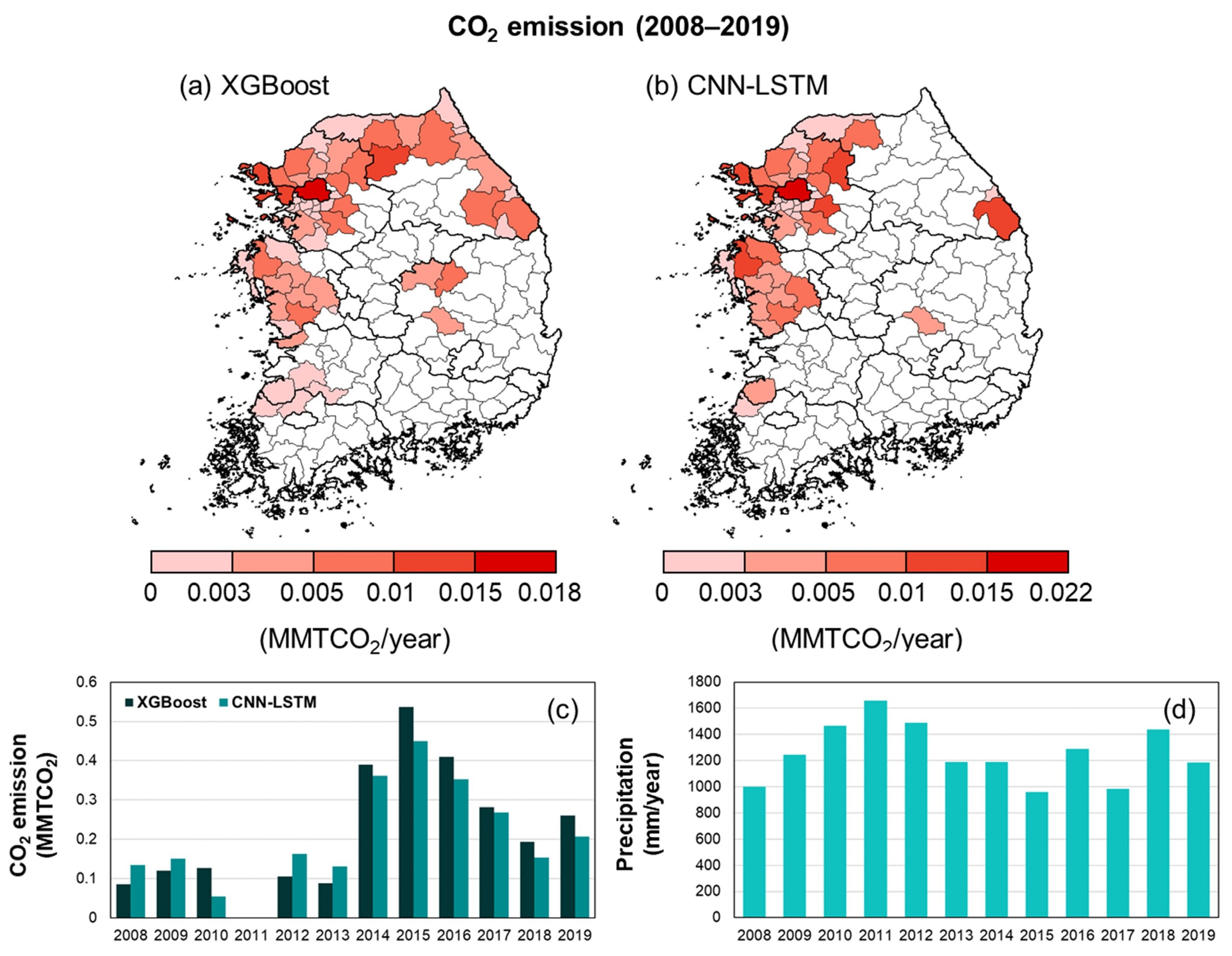
Atmospheric CO2 emissions resulting from groundwater storage depletion were estimated using Equation (5). For these calculations, only the model-predicted groundwater storage depletions and the -derived equivalent CO2 concentrations for 2008–2019 were used, because bicarbonate concentration data from the NGMN in Korea have been available only since 2008. A comparison of the CO2 emission estimates between XGBoost and CNN-LSTM revealed consistent emission patterns, as shown in Figure 9a,b. Both models estimated GWSA values below approximately –200 mm/year in the northwestern A01, A02, and A03 provinces and the eastern A05 province (see Figure 8c,d). Furthermore, a significant decrease was noted in groundwater storage in these provinces, contributing to CO2 emissions. Notably, Seoul, the capital of Korea, releases more than 0.015 MMT CO2/year, the highest level identified by both models.
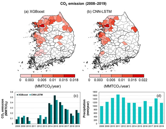
Figure 9.
CO2 emissions due to groundwater storage depletion estimated by (a) XGBoost and (b) CNN-LSTM. (c) Annual CO2 emissions. (d) Annual precipitation in South Korea.
The CO2 emissions estimated by XGBoost and CNN-LSTM were approximately 0.216 and 0.202 MMTCO2/year during 2008–2019, respectively. The yearly total CO2 emissions (2008–2019) are compared between XGBoost and CNN-LSTM in Figure 9c. Emissions for 2011 were excluded because NGMN did not provide the corresponding bicarbonate concentration data. XGBoost and CNN-LSTM estimated the total cumulative CO2 emissions for 2008–2019 to be 2.596 and 2.426 MMTCO2, respectively. From 2012 to 2015, a gradual increase in CO2 emissions was observed, which can be attributed to a corresponding decrease in precipitation during the same period (Figure 9c,d).
4.3. Evaluation of Groundwater Storage Depletion and CO2 Emission Vulnerability
Figure 10 shows the weights of the six indicators for vulnerability estimation using the entropy weight method. The weights were calculated separately for GWSA predictions using XGBoost and CNN-LSTM and were similar in both cases. The water supply ratio had the highest weight (0.351–0.358), followed by groundwater use per unit area (0.246–0.251), cultivation land per unit area (0.204–0.209), GWSA (0.094–0.113), non-rainy days (0.057–0.058), and finally precipitation (0.029–0.030). The use of the entropy weight method resulted in the positive and negative indicators being weighted at 50% each, indicating that indicator selection was appropriate. The water supply ratio had the highest weight due to its relatively low variance, indicating considerable agglomeration. In contrast, non-rainy days and precipitation had lower weights because their values vary widely across administrative regions in Korea, resulting in low agglomeration. With regard to GWSA, CNN-LSTM had a higher weight than XGBoost did, which is considered to be due to the difference in magnitudes between the XGBoost-predicted and CNN-LSTM-predicted GWSA (Figure 8c,d).
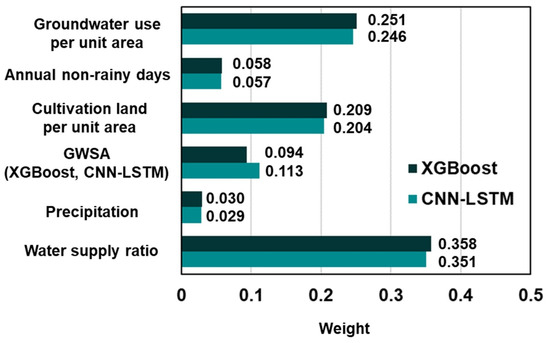
Figure 10.
Weights of six indicators determined using the entropy weight method.
Vulnerability to groundwater storage depletion was evaluated in each administrative region of all provinces using TOPSIS based on the entropy weight method (entropy–TOPSIS). Vulnerability was classified into five levels (very low, low, moderate, high, and very high) based on the closeness coefficient estimates obtained from TOPSIS using the geometric interval function of the ArcGIS tool. The vulnerability maps prepared using the XGBoost and CNN-LSTM predictions are shown in Figure 11.
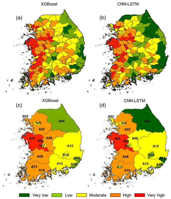
Figure 11.
Groundwater storage depletion vulnerability maps prepared using the entropy–TOPSIS method for each administrative region ((a) XGBoost; (b) CNN-LSTM) and province ((c) XGBoost; (d) CNN-LSTM).
Both vulnerability maps highlight a relatively large area in the western region as having very high vulnerability. By comparison, the vulnerability of a large proportion of the eastern regions was observed to be low or very low. The higher vulnerability to groundwater storage depletion in the western regions is visually consistent with the spatial distribution of GWSA (Figure 8c,d) and its trends (Figure 8a,b), which exhibited a decreasing pattern in these regions.
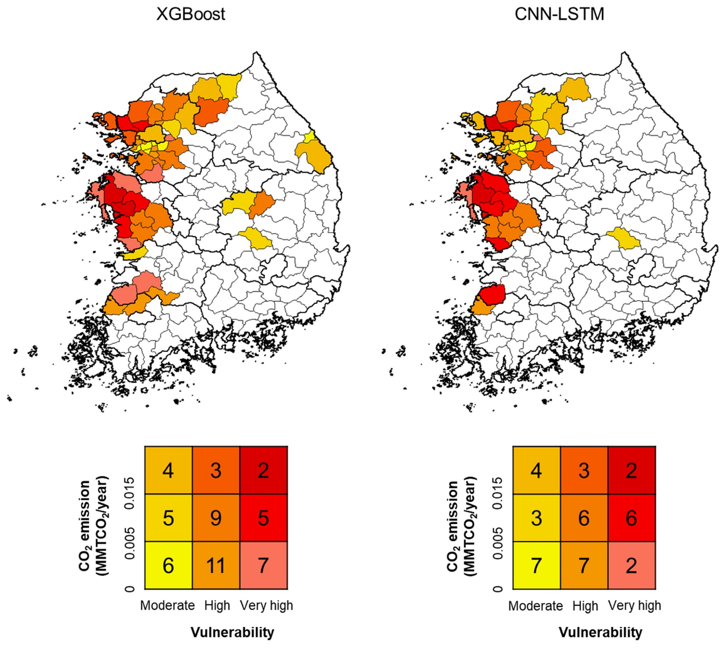
Figure 12 presents maps depicting the co-occurrence of CO2 emissions resulting from groundwater storage depletion (Figure 9a,b) and vulnerability (Figure 11) to groundwater storage depletion; the legend shows the counts of the corresponding regions. These maps reveal that over 80% of the administrative regions that experienced CO2 emissions due to groundwater storage depletion also exhibited moderate, high, or very high vulnerability to groundwater storage depletion. Based on the XGBoost and CNN-LSTM predictions, we respectively identified 52 and 40 administrative regions as hotspots, representing potential areas that are highly vulnerable to groundwater storage depletion and consequent CO2 emissions (legends in Figure 12).
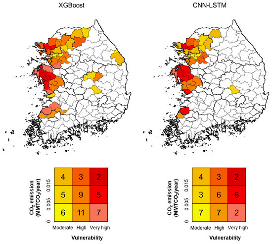
Figure 12.
Co-occurrence of CO2 emissions and groundwater storage depletion vulnerability (the legends show the number of corresponding administrative regions).
5. Discussion
5.1. Groundwater Storage Depletion Using Data-Driven Models Based on Multi-Satellite and Reanalysis Data
Recent research has shown that groundwater storage depletion impacts atmospheric CO2 emissions, underscoring the importance of identifying spatiotemporal groundwater storage depletion and monitoring the associated CO2 emissions. Estimating CO2 emissions resulting from groundwater storage depletion necessitates a precise assessment of changes in groundwater storage, along with the trends and magnitudes of depletion. The GRACE satellite, in conjunction with GLDAS and other satellite-based hydrologic components, has enabled the monitoring of global groundwater changes [64,65]. Various studies have conducted comprehensive assessments of groundwater storage depletion using GRACE data. For instance, Ramjeawon et al. [8] reported a net groundwater storage depletion of 9.25 × 10⁸ m3/year (141.87 mm/year) for the Usutu-Mhlatuze region (6520 km2) in South Africa from 2002 to 2021 based on GRACE data. Similarly, Mohammed et al. [9] documented groundwater storage depletion in the Arabian Peninsula, estimating a depletion of 87.6–96.61 mm/year from 2002 to 2020. Previous methods primarily utilized the water balance equation to estimate groundwater storage depletion [11,64,65]. In this study, we developed a data-driven model to predict GWSA and groundwater storage depletion by innovatively integrating GRACE data, reanalysis data (GLDAS), and satellite-derived (TRMM and Landsat) hydrological data.
We predicted spatiotemporal GWSA in South Korea and groundwater storage depletion through the trend test. The average groundwater storage depletion for the period between 2008 and 2019 of the XGBoost and CNN-LSTM models is 148.78 mm/year and 254.11 mm/year, respectively. Overall, the statistical results indicate that the model GWSA predictions and in situ observations were in agreement. Both XGBoost and CNN-LSTM provided relatively accurate predictions, not only temporally but also spatially. Consistent with our findings, other researchers have demonstrated the effectiveness of machine and deep learning models in accurately predicting groundwater storage [17,18,19]. The XGBoost model outperformed the CNN-LSTM model overall, particularly in the southeast region, where the CNN-LSTM model had a higher RMSE. The accuracy of the models in this region was relatively low because of the complexity of the coastal area, where groundwater levels fluctuate more than in the other regions. To address the relatively large errors in this region, it will be necessary to enhance the model by incorporating various input data or further tuning hyperparameters.
5.2. Relationships between Groundwater Storage Depletion-Associated CO2 Emissions and Vulnerability
Using the spatiotemporal GWSA predicted by data-driven models, CO2 emissions due to groundwater storage depletion in South Korea from 2008 to 2019 were estimated. Although the emissions (0.202–0.216 MMTCO2/year) are lower than those of the United States (~1.7 MMTCO2/year; [12]) and India (~0.72 MMTCO2/year; [16]), they are considered relatively high given South Korea’s significantly smaller area compared to these countries. Notably, the highest annual CO2 emissions were recorded in 2015, with estimated values of 0.537 and 0.450 MMTCO2 for XGBoost and CNN-LSTM, respectively, concurring with precipitation being lowest that year (Figure 9d). This follows the assumption that a decrease in precipitation reduces groundwater storage, which consequently increases CO2 emissions. Further research is required to investigate the relationship among droughts resulting from reduced precipitation, water scarcity, and CO2 emissions.
Additionally, we analyzed regions vulnerable to groundwater storage depletion to identify potential hotspots of the associated CO2 emissions. As observed in Figure 11, the western regions (A02, A03, A05, A08, and A09 provinces) constitute a large proportion (~ 50%) of the areas with high and very high vulnerability. In contrast, the eastern regions (A04, A15, and A16 provinces) cover more areas with low and very low vulnerability. The vulnerability of province A05 was classified as very high (Figure 11c,d); this province contains the largest proportion of vulnerable areas (Figure 11a,b). These areas predominantly consist of agricultural cultivation zones, which have a low water supply ratio compared with that of other regions, indicating high groundwater usage. Province A05 has been severely affected by recent droughts, which have exacerbated its vulnerability by reducing groundwater recharge and forcing increased groundwater extraction.
In addition, numerous co-occurrences of areas with high CO2 emissions and vulnerabilities are observed in the western region, particularly in the A02, A03, and A05 provinces. Notably, 70% of the total area in the A05 province showcased co-occurrences of higher CO2 emissions and high or very high vulnerability (Figure 12). Our findings indicate that the western regions (A02, A03, and A05 provinces) of South Korea are particularly susceptible to groundwater storage depletion and the associated potential risk of CO2 emissions.
5.3. Significance and Limitations
Point measurements of groundwater are insufficient to identify spatiotemporal changes in GWSA, groundwater storage depletion, and their associated CO2 emissions. The data-driven model developed in this study can analyze and predict GWSA changes and groundwater storage depletion across different temporal and spatial scales. This approach is expected to play a crucial role in understanding future trends, variations, and patterns of groundwater availability. However, the GWSA prediction results from this model have a spatial resolution of 0.25°, which limits the analysis of groundwater dynamics in detail. Therefore, future research should consider applying methods such as downscaling to improve resolution. It is necessary to employ various data-driven models utilizing a range of precise satellite data to enhance the accuracy of groundwater-related issue assessments. Furthermore, integrating advanced data-driven models and incorporating more comprehensive datasets will be essential to refine predictions and better capture the complexities of groundwater systems.
This study is significant as it represents the first effort in Korea to estimate CO2 emissions resulting from groundwater storage depletion. Table 5 shows the average CO2 emissions in Inventories of South Korea (2008–2019; https://kosis.kr/, accessed on 1 July 2024). CO2 emissions due to groundwater storage may account for a small portion of total CO2 emissions compared to other sectors, but it is imperative to include groundwater-related activities in considering carbon fluxes. The CO2 emissions from groundwater storage depletion are also higher than those from crop residue burning and are comparable to emissions from wetlands and waste (etc.). Therefore, the CO2 emissions resulting from groundwater storage depletion are significant and should not be overlooked. Additionally, recognizing the substantial impact of groundwater depletion on carbon emissions underscores the importance of groundwater management practices to mitigate climate change. These insights can inform groundwater management decisions and future CO2 emission inventories in South Korea.
Table 5.
Average CO2 Emissions in Inventories of South Korea (2008–2019).
Additionally, this study analyzed the relationship between groundwater storage depletion-associated CO2 emissions and vulnerability. It reveals that western areas experienced high vulnerability to groundwater storage depletion and concurrent CO2 emissions. This finding demonstrates a correlation between groundwater storage depletion vulnerability and associated CO2 emissions. Furthermore, the insights gained from this study can assist the decision-making process and resource management strategies aimed at mitigating both groundwater storage depletion and its impact on CO2 emissions.
In this study, only CO2 emissions resulting from the depletion of GWSA were estimated. The impact of groundwater storage depletion on CO2 emissions is driven by a variety of mechanisms. As groundwater levels decline, water must be pumped from greater depths, requiring more energy. This increase in energy consumption often relies on fossil fuels, which leads to higher CO2 emissions. For instance, Kazakis et al. [66] quantified groundwater depletion in aquifers in the Eastern Thermaikos Gulf, Mouriki, and Marathonas basins in Greece, and explored the application of managed aquifer recharge (MAR) to address groundwater depletion and reduce associated CO2 emissions. They also proposed approaches economically to reverse groundwater storage depletion by MAR operation scenarios and strategies to mitigate the impacts of groundwater storage depletion. Consequently, various analyses and strategies are needed to mitigate groundwater storage depletion and the resulting CO2 emissions.
Groundwater storage depletion can also reduce irrigation water availability, impacting crop yields, and stressing natural vegetation, especially in arid and semi-arid regions, leading to additional CO2 emissions. Furthermore, groundwater storage depletion can reduce the extent of wetlands, which are significant carbon sinks, causing stored carbon to be released as CO2 or methane (CH4). Therefore, understanding the future impact of groundwater storage depletion on CO2 emissions will require a detailed analysis of the relationship between carbon and the hydrological cycle.
6. Conclusions
Groundwater storage depletion has recently been identified as a source of atmospheric CO2 emission. The fact that it is considered one of the top 20 sources in the USA, along with major sources such as fossil fuel combustion and non-energy use of fuels, implies that CO2 emissions due to groundwater depletion must be accounted for in future CO2 budgets.
Key conclusions drawn from this study include
- Data-driven models based on multi-satellite and reanalysis data can predict spatiotemporal GWSA with relatively high accuracy.
- CO2 emissions from groundwater storage depletion in South Korea were estimated to be 0.216 and 0.202 MMTCO2/year using XGBoost and CNN-LSTM models, respectively.
- Western regions of South Korea are highly or very highly vulnerable to groundwater storage depletion and prone to CO2 emissions.
- A correlation relationship was identified between the co-occurrence of CO2 emissions from groundwater storage depletion and vulnerability to groundwater storage depletion.
Author Contributions
Conceptualization, J.Y.S. and S.-I.L.; Data curation, J.Y.S.; Formal analysis, J.Y.S.; Funding acquisition, J.Y.S. and S.-I.L.; Methodology, J.Y.S.; Resources, S.-I.L.; Software, J.Y.S.; Supervision, S.-I.L.; Validation, J.Y.S.; Visualization, J.Y.S.; Writing—original draft, J.Y.S.; Writing—review and editing, J.Y.S. and S.-I.L. All authors have read and agreed to the published version of the manuscript.
Funding
This work was supported by a National Research Foundation of Korea (NRF) grant funded by the Korean government (MSIT) (No. NRF-2022R1C1C2004417).
Data Availability Statement
The original contributions presented in the study are included in the article, further inquiries can be directed to the corresponding author.
Acknowledgments
The authors would like to express our gratitude to the editors and reviewers for their constructive comments and suggestions.
Conflicts of Interest
The authors declare no conflicts of interest.
References
- IPCC. Global Warming of 1.5 °C. An IPCC Special Report on the Impacts of Global Warming of 1.5 °C above Pre-Industrial Levels and Related Global Greenhouse Gas Emission Pathways, in the Context of Strengthening the Global Response to the Threat of Climate Change, Sustainable Development, and Efforts to Eradicate Poverty; Cambridge University Press: Cambridge, UK; New York, NY, USA, 2018. [Google Scholar] [CrossRef]
- Fawzy, S.; Osman, A.I.; Doran, J.; Rooney, D.W. Strategies for Mitigation of Climate Change: A Review. Environ. Chem. Lett. 2020, 18, 2069–2094. [Google Scholar] [CrossRef]
- Armour, K.C. Energy Budget Constraints on Climate Sensitivity in Light of Inconstant Climate Feedbacks. Nat. Clim. Chang. 2017, 7, 331–335. [Google Scholar] [CrossRef]
- Ahlström, A.; Raupach, M.R.; Schurgers, G.; Smith, B.; Arneth, A.; Jung, M.; Reichstein, M.; Canadell, J.G.; Friedlingstein, P.; Jain, A.K.; et al. The Dominant Role of Semi-Arid Ecosystems in the Trend and Variability of the Land CO2 Sink. Science 2015, 348, 895–899. [Google Scholar] [CrossRef] [PubMed]
- Raymond, P.A.; Hartmann, J.; Lauerwald, R.; Sobek, S.; McDonald, C.; Hoover, M.; Butman, D.; Striegl, R.; Mayorga, E.; Humborg, C.; et al. Global Carbon Dioxide Emissions from Inland Waters. Nature 2013, 503, 355–359. [Google Scholar] [CrossRef] [PubMed]
- Jasechko, S.; Seybold, H.; Perrone, D.; Fan, Y.; Shamsudduha, M.; Taylor, R.G.; Fallatah, O.; Kirchner, J.W. Rapid Groundwater Decline and Some Cases of Recovery in Aquifers Globally. Nature 2024, 625, 715–721. [Google Scholar] [CrossRef]
- Castellazzi, P.; Garfias, J.; Martel, R. Assessing the Efficiency of Mitigation Measures to Reduce Groundwater Depletion and Related Land Subsidence in Querétaro (Central Mexico) from Decadal InSAR Observations. Int. J. Appl. Earth Obs. Geoinf. 2021, 105, 102632. [Google Scholar] [CrossRef]
- Ramjeawon, M.; Demlie, M.; Toucher, M. Analyses of Groundwater Storage Change Using GRACE Satellite Data in the Usutu-Mhlatuze Drainage Region, North-Eastern South Africa. J. Hydrol. Reg. Stud. 2022, 42, 101118. [Google Scholar] [CrossRef]
- Mohamed, A.; Alarifi, S.S.; Mohammed, M.A.A. Geophysical Monitoring of the Groundwater Resources in the Southern Arabian Peninsula Using Satellite Gravity Data. Alex. Eng. J. 2024, 86, 311–326. [Google Scholar] [CrossRef]
- Zhang, X.; Jiang, L.; Liu, Z.; Kittel, C.M.M.; Yao, Z.; Druce, D.; Wang, R.; Tøttrup, C.; Liu, J.; Jiang, H.; et al. Flow Regime Changes in the Lancang River, Revealed by Integrated Modeling with Multiple Earth observation Datasets. Sci. Total Environ. 2023, 862, 160656. [Google Scholar] [CrossRef]
- Rodell, M.; Velicongna, I.; Famiglietti, J.S. Satellite-Based Estimates of Groundwater Depletion in India. Nature 2009, 460, 999–1002. [Google Scholar] [CrossRef]
- Wood, W.W.; Hyndman, D.W. Groundwater Depletion: A Significant Unreported Source of Atmospheric Carbon Dioxide. Earths Future 2017, 5, 1133–1135. [Google Scholar] [CrossRef]
- Macpherson, G.L. CO2 Distribution in Groundwater and the Impact of Groundwater Extraction on the Global C Cycle. Chem. Geol. 2009, 264, 328–336. [Google Scholar] [CrossRef]
- Rajan, A.; Ghosh, K.; Shah, A. Carbon Footprint of India’s Groundwater Irrigation. Caron Manag. 2020, 11, 265–280. [Google Scholar] [CrossRef]
- US EPA, Inventory of U.S. Greenhouse Gas Emissions and Sinks: 1990–2014; U.S. Environmental Protection Agency: Washington, DC, USA, 2016.
- Mishra, V.; Asoka, A.; Vatta, K.; Lall, U. Groundwater Depletion Associated CO2 Emissions in India. Earths Future 2018, 6, 1672–1681. [Google Scholar] [CrossRef]
- Rohde, M.M.; Biswas, T.; Housman, I.W.; Campbell, L.S.; Klausmeyer, K.R.; Howard, J.K. A Machine Learning Approach to Predict Groundwater Levels in California Reveals Ecosystems at Risk. Front. Earth Sci. 2021, 9, 784499. [Google Scholar] [CrossRef]
- Seo, J.Y.; Lee, S.-I. Predicting Changes in Spatiotemporal Groundwater Storage through the Integration of Multi-Satellite Data and Deep Learning Models. IEEE Access 2021, 9, 15757–157583. [Google Scholar] [CrossRef]
- Wunsch, A.; Liesch, T.; Broda, S. Deep Learning shows Declining Groundwater Levels in Germany until 2100 due to Climate Change. Nat. Commun. 2022, 13, 1221. [Google Scholar] [CrossRef] [PubMed]
- Jaafarzadeh, M.S.; Tahmasebipour, N.; Haghizadeh, A.; Pourghasemi, H.R.; Rouhani, H. Groundwater Recharge Potential Zonation using an Ensemble of Machine Learning and Bivariate Statistical Models. Sci. Rep. 2021, 11, 5587. [Google Scholar] [CrossRef]
- Arabameri, A.; Pal, S.C.; Rezaie, F.; Nalivan, O.A.; Chowdhuri, I.; Saha, A.; Lee, S.; Moayedi, H. Modeling Groundwater Potential Using Novel GIS-Based Machine-Learning Ensemble Techniques. J. Hydrol. Reg. Stud. 2021, 36, 100848. [Google Scholar] [CrossRef]
- Madani, A.; Niyazi, B. Groundwater Potential Mapping Using Remote Sensing and Random Forest Machine Learning Model: A Case Study from Lower Part of Wadi Yalamlam, Western Saudi Arabia. Sustainability 2023, 15, 2772. [Google Scholar] [CrossRef]
- Ali, S.; Liu, D.; Fu, Q.; Cheema, M.J.M.; Pal, S.C.; Arshad, A.; Pham, Q.B.; Zhang, L. Constructing High-Resolution Groundwater Drought at Spatio-Temporal Scale Using GRACE Satellite Data based on Machine Learning in the Indus Basin. J. Hydrol. 2022, 612, 128295. [Google Scholar] [CrossRef]
- Seo, J.Y.; Lee, S.-I. Probabilistic Evaluation of Drought Propagation Using Satellite Data and Deep Learning Model: From Precipitation to Soil Moisture and Groundwater. IEEE J. Sel. Top. Appl. Earth Obs. Remote Sens. 2023, 16, 6048–6061. [Google Scholar] [CrossRef]
- Zhu, R.; Zheng, H.; Jakeman, A.J.; Chiew, F.H.S. Multi-Timescale Performance of Groundwater Drought in Connection with Climate. Water Resour. Manag. 2023, 37, 3599–3614. [Google Scholar] [CrossRef]
- Sabzehee, F.; Amiri-Simkooei, A.R.; Iran-Pour, S.; Vishwakarma, B.D.; Kerachian, R. Enhancing Spatial Resolution of GRACE-Derived Groundwater Storage Anomalies in Urmia Catchment Using Machine Learning Downscaling Methods. J. Environ. Manag. 2023, 330, 117180. [Google Scholar] [CrossRef] [PubMed]
- Agarwal, V.; Akyilmaz, O.; Shum, C.K.; Feng, W.; Yang, T.-Y.; Forootan, E.; Syed, T.H.; Haritashya, U.K.; Uz, M. Machine Learning based Downscaling of GRACE-Estimated Groundwater in Central Valley, California. Sci. Total Environ. 2023, 865, 161138. [Google Scholar] [CrossRef]
- Wang, J.; Xu, D.; Li, H. Constructing GRACE-Based 1 km Resolution Groundwater Storage Anomalies in Arid Regions Using an Improved Machine Learning Downscaling Method: A Case Study in Alxa League, China. Remote Sens. 2023, 15, 2913. [Google Scholar] [CrossRef]
- Yang, W.; Xu, K.; Lian, J.; Ma, C.; Bin, L. Integrated Flood Vulnerability Assessment Approach based on TOPSIS and Shannon Entropy Methods. Ecol. Indic. 2018, 89, 269–280. [Google Scholar] [CrossRef]
- IPCC. Climate Change 2001: Impacts, Adaptation, and Vulnerability. Contribution of Working Group II to the Third Assessment Report of the Intergovernmental Panel on Climate Change; Cambridge University Press: Cambridge, UK; New York, NY, USA, 2001. [Google Scholar]
- Adger, W.N. Vulnerability. Glob. Environ. Change 2006, 16, 268–281. [Google Scholar] [CrossRef]
- Koo, M.-S.; Hong, S.-Y.; Kim, J. An Evaluation of the Tropical Rainfall Measuring Mission (TRMM) Multi-Satellite Precipitation Analysis (TMPA) Data over South Korea. Asia Pac. J. Atmos. Sci. 2009, 45, 265–282. [Google Scholar]
- Seo, J.Y.; Lee, S.-I. Total Discharge Estimation in the Korean Peninsula Using Multi-Satellite Products. Water. 2017, 9, 532. [Google Scholar] [CrossRef]
- Rodell, M.; Houser, P.R.; Jambor, U.; Gottschalck, J.; Mitchell, K.; Meng, C.-J.; Arsenault, K.; Cosgrove, B.; Radakovich, J.; Bosilovich, M.; et al. The Global Land Data Assimilation System. Bull. Am. Meteorol. Soc. 2004, 85, 381–394. [Google Scholar] [CrossRef]
- Cooley, T.; Anderson, G.P.; Felde, G.W.; Hoke, M.L.; Ratkowski, A.J.; Chetwynd, J.H.; Gardner, J.A.; Adler-Golden, S.M.; Matthew, M.W.; Berk, A.; et al. FLAASH, a MODTRAN4-Based Atmospheric Correction Algorithm, Its Application and Validation. In Proceedings of the IEEE International Symposium on Geoscience Remote Sensing, Toronto, ON, Canada, 24–28 June 2002. [Google Scholar] [CrossRef]
- Tapley, B.D.; Bettadpur, S.; Watkins, M.; Reigber, C. The Gravity Recovery and Climate Experiment: Mission Overview and Early Result. Geophys. Res. Lett. 2004, 31, L09607. [Google Scholar] [CrossRef]
- Save, H.; Bettadpur, S.; Tapley, B.D. High Resolution CSR GRACE RL05 Mascons. J. Geophys. Res. Solid Earth 2016, 121, 7547–7569. [Google Scholar] [CrossRef]
- Save, H. CSR GRACE and GRACE-FO RL06 Mascon Solutions v02. Available online: https://www2.csr.utexas.edu/grace/RL06_mascons.html (accessed on 20 November 2023).
- Wang, S.; Cui, G.; Li, X.; Liu, Y.; Li, X.; Tong, S.; Zhang, M. GRACE Satellite-Based Analysis of Spatiotemporal Evolution and Driving Factors of Groundwater Storage in the Black Soil Region of Northeast China. Remote Sens. 2023, 15, 704. [Google Scholar] [CrossRef]
- Cho, Y. Analysis of Terrestrial Water Storage Variations in South Korea Using GRACE Satellite and GLDAS Data in Google Earth Engine. Hydrol. Sci. J. 2024, 69, 1032–1045. [Google Scholar] [CrossRef]
- Guo, J.; Li, W.; Chnag, X.; Zhu, G.; Liu, X.; Guo, B. Terrestrial Water Storage Changes over Xinjiang Extracted by Combining Gaussian Filter and Multichannel Singular Spectrum Analysis from GRACE. Geophys. J. Int. 2018, 213, 397–407. [Google Scholar] [CrossRef]
- Nigatu, Z.M.; Fan, D.; You, W.; Melesse, A.M. Hydroclimatic Extremes Evaluation Using GRACE/GRACE-FO and Multidecadal Climatic Variables over the Nile River Basin. Remote Sens. 2021, 13, 651. [Google Scholar] [CrossRef]
- Qu, W.; Jin, Z.; Zhang, Q.; Gao, Y.; Zhang, P.; Chen, P. Estimation of Evapotranspiration in the Yellow River Basin from 2002 to 2020 based on GRACE and GRACE Follow-On Observations. Remote Sens. 2022, 14, 730. [Google Scholar] [CrossRef]
- Shi, Z.; Zheng, W.; Yin, W. Improving the Reliability of the Prediction of Terrestrial Water Storage in Yunnan Using the Artificial Neural Network Selective Joint Prediction Model. IEEE Access 2021, 9, 31865–31879. [Google Scholar] [CrossRef]
- Johnson, A.I. Specific Yield: Compilation of Specific Yields for Various Materials; Water Supply Paper, 1662-D; U.S. Government Printing Office: Washington, DC, USA, 1967; pp. D1–D70. [Google Scholar]
- Loheide, S.P., II; Butler, J.J., Jr.; Gorelick, S.M. Estimation of Groundwater Consumption by Phreatophytes Using Diurnal Water Table Fluctuations: A Saturated-Unsaturated Flow Assessment. Water Resour. Res. 2005, 41, W07030. [Google Scholar] [CrossRef]
- Niazkar, M.; Menapace, A.; Brentan, B.; Piraei, R.; Jimenez, D.; Dhawan, P.; Righetti, M. Applications of XGBoost in Water Resources Engineering: A Systematic Literature Review (Dec 2018–May 2023). Environ. Model. Softw. 2024, 174, 105971. [Google Scholar] [CrossRef]
- Yang, R.; Singh, S.K.; Tavakkoli, M.; Amiri, N.; Yang, Y.; Karami, M.A.; Rai, R. CNN-LSTM Deep Learning Architecture for Computer Vision-Based Modal Frequency Detection. Mech. Syst. Signal Process. 2020, 144, 106885. [Google Scholar] [CrossRef]
- Wu, J.; Chen, X.-Y.; Zhang, H.; Xiong, L.-D.; Lei, H.; Deng, S.-H. Hyperparameter Optimization for Machine Learning Models based on Bayesian Optimization. J. Electron. Sci. Technol. 2019, 17, 26–40. [Google Scholar] [CrossRef]
- Gilbert, R.O. Statistical Methods for Environmental Pollution Monitoring; Van Nostrand Reinhold: New York, NY, USA, 1987. [Google Scholar]
- Sen, P.K. Estimates of the Regression Coefficient based on Kendall’s Tau. J. Am. Stat. Assoc. 1968, 63, 1379–1389. [Google Scholar] [CrossRef]
- Yue, S.; Wang, C.Y. Applicability of Prewhitening to Eliminate the Influence of Serial Correlation on the Mann-Kendall Test. Water Resour. Res. 2002, 38, 4-1–4-7. [Google Scholar] [CrossRef]
- Collaud Coen, M.; Andrews, E.; Bigi, A.; Martucci, G.; Romanens, G.; Vogt, F.P.A.; Vuilleumier, L. Effects of the Prewhitening Method, the Time Granularity, and the Time Segmentation on the Mann–Kendall Trend Detection and the Associated Sen’s slope. Atmos. Meas. Tech. 2020, 13, 6945–6964. [Google Scholar] [CrossRef]
- Hwang, C.-L.; Yoon, K. Methods for multiple attribute decision making. In Multiple Attribute Decision Making: Methods and Applications; Lecture Notes in Economics and Mathematical Systems; Springer: Berlin/Heidelberg, Germany, 1981; pp. 58–191. [Google Scholar]
- Sahana, V.; Mondal, A.; Sreekumar, P. Drought Vulnerability and Risk Assessment in India: Sensitivity Analysis and Comparison of Aggregation Techniques. J. Environ. Manag. 2021, 299, 113689. [Google Scholar] [CrossRef]
- Shin, H.; Lee, G.; Lee, J.; Lee, J.; Park, M.; Park, C. An Approach to Drought Vulnerability Assessment Focused on Groundwater Wells in Upland Cultivation Areas of South Korea. Agronomy 2021, 11, 1783. [Google Scholar] [CrossRef]
- Meshram, S.G.; Alvandi, E.; Meshram, C.; Kahya, E.; AI-Quraishi, A.M.F. Application of SAW and TOPSIS in Prioritizing Watersheds. Water Resour. Manag. 2020, 34, 715–732. [Google Scholar] [CrossRef]
- Pathan, A.I.; Agnihotri, P.G.; Said, S.; Patel, D. AHP and TOPSIS based Flood Risk Assessment-A Case Study of the Navsari City, Gujarat, India. Environ. Monit. Assess. 2022, 194, 509. [Google Scholar] [CrossRef]
- Shafiei Shiva, J.; Chandler, D.G.; Kunkel, K.E. Mapping Heat Wave Hazard in Urban Areas: A Novel Multi-Criteria Decision Making Approach. Atmosphere 2022, 13, 1037. [Google Scholar] [CrossRef]
- Zong, J.; Wang, L.; Lu, C.; Du, Y.; Wang, Q. Mapping Health Vulnerability to Short-Term Summer Heat Exposure based on a Directional Interaction Network: Hotspots and Coping Strategies. Sci. Total Environ. 2023, 881, 163401. [Google Scholar] [CrossRef]
- Shannon, C.E. A Mathematical Theory of Communication. Bell Syst. Tech. J. 1948, 27, 379–423. [Google Scholar] [CrossRef]
- Shannon, C.E. A Mathematical Theory of Communication. Bell Syst. Tech. J. 1948, 27, 623–656. [Google Scholar] [CrossRef]
- Méndez, M.; Galván, B.; Salazar, D.; Greiner, D. Multiple-Objective Genetic Algorithm Using the Multiple Criteria Decision Making Method TOPSIS. In Lecture Notes in Economics and Mathematical Systems; Barichard, V., Ehrgott, M., Gandibleux, X., T’Kindt, V., Eds.; Springer: Berlin/Heidelberg, Germany, 2009; pp. 145–154. [Google Scholar]
- Gautam, P.K.; Chandra, S.; Henry, P.K. Monitoring of the Groundwater Level Using GRACE with GLDAS Satellite Data in Ganga Plain, India to Understand the Challenges of Groundwater, Depletion, Problems, and Strategies for Mitigation. Environ. Chall. 2024, 15, 100874. [Google Scholar] [CrossRef]
- Panday, D.P.; Kumar, M. Application of Remote Sensing Techniques to Deal with Scale Aspects of GRACE Data to Quantify Groundwater Levels. MethodsX 2023, 10, 102108. [Google Scholar] [CrossRef] [PubMed]
- Kazakis, N.; Karakatsanis, D.; Ntona, M.M.; Polydoropoulos, K.; Zavridou, E.; Voudouri, K.A.; Busico, G.; Kalaitzidou, K.; Patsialis, T.; Perdikaki, M.; et al. Groundwater Depletion. Are Environmentally Friendly Energy Recharge Dams a Solution? Water 2024, 16, 1541. [Google Scholar] [CrossRef]


Disclaimer/Publisher’s Note: The statements, opinions and data contained in all publications are solely those of the individual author(s) and contributor(s) and not of MDPI and/or the editor(s). MDPI and/or the editor(s) disclaim responsibility for any injury to people or property resulting from any ideas, methods, instructions or products referred to in the content. |
© 2024 by the authors. Licensee MDPI, Basel, Switzerland. This article is an open access article distributed under the terms and conditions of the Creative Commons Attribution (CC BY) license (https://creativecommons.org/licenses/by/4.0/).