MLF-PointNet++: A Multifeature-Assisted and Multilayer Fused Neural Network for LiDAR-UAS Point Cloud Classification in Estuarine Areas

Abstract

LiDAR-unmanned aerial system (LiDAR-UAS) technology can accurately and efficiently obtain detailed and accurate three-dimensional spatial information of objects. The classification of objects in estuarine areas is highly important for management, planning, and ecosystem protection. Owing to the presence of slopes in estuarine areas, distinguishing between dense vegetation (lawns and trees) on slopes and the ground at the tops of slopes is difficult. In addition, the imbalance in the number of point clouds also poses a challenge for accurate classification directly from point cloud data. A multifeature-assisted and multilayer fused neural network (MLF-PointNet++) is proposed for LiDAR-UAS point cloud classification in estuarine areas. First, the 3D shape features that characterize the geometric characteristics of targets and the visible-band difference vegetation index (VDVI) that can characterize vegetation distribution are used as auxiliary features to enhance the distinguishability of dense vegetation (lawns and trees) on slopes and the ground at the tops of slopes. Second, to enhance the extraction of target spatial information and contextual relationships, the feature vectors output by different layers of set abstraction in the PointNet++ model are fused to form a combined feature vector that integrates low and high-level information. Finally, the focal loss function is adopted as the loss function in the MLF-PointNet++ model to reduce the effect of imbalance in the number of point clouds in each category on the classification accuracy. A classification evaluation was conducted using LiDAR-UAS data from the Moshui River estuarine area in Qingdao, China. The experimental results revealed that MLF-PointNet++ had an overall accuracy (OA), mean intersection over union (mIOU), kappa coefficient, precision, recall, and F₁-score of 0.976, 0.913, 0.960, 0.953, 0.953, and 0.953, respectively, for object classification in the three representative areas, which were better than the corresponding values for the classification methods of random forest, BP neural network, Naive Bayes, PointNet, PointNet++, and RandLA-Net. The study results provide effective methodological support for the classification of objects in estuarine areas and offer a scientific basis for the sustainable development of these areas.

1. Introduction

An estuarine area is an intersection of rivers, oceans, or lakes and is defined as a “semienclosed coastal water body that is permanently or regularly connected to the ocean [1]”. This also makes estuarine areas among the most ecologically, socially, and culturally rich ecosystems [2]. However, the environment in these areas is constantly changing due to river erosion, sedimentation, vegetation growth, and human activities [3], and at the same time, a complex variety of terrain types in estuarine areas have emerged. Accurate classification of estuarine areas can reflect environmental conditions and reveal spatiotemporal evolution patterns, playing an important role in economic development and ecological monitoring [4].

With the continuous development of remote sensing technology, airborne laser detection and ranging systems have provided a new technical approach for obtaining three-dimensional spatial data. As an active remote sensing technology, LiDAR-UAS has the advantages of fast measurement speed, high measurement accuracy, and is not affected by lighting conditions [5]. Owing to the large number of mudflats and complex terrain in estuarine areas, surveyors in river channel areas are unable to access these areas. Using LiDAR-UAS for scanning not only overcomes environmental limitations but also quickly obtains surface information in these areas. In recent years, this technique has been applied more often in fields such as island reef mapping [6], digital 3D reconstruction [7] forest monitoring [8], and cultural heritage protection.

LiDAR-UAS point cloud data have unique advantages in terrain measurement and object classification in estuarine areas. The methods for classifying LiDAR-UAS point clouds can be categorized into traditional feature analysis methods, machine learning methods, and deep learning methods. Traditional feature analysis methods segment the regional point cloud by analyzing the features of neighboring points and then perform recognition and classification of point cloud targets through prior knowledge. On the basis of prior knowledge, Sithole et al. [9] used line segment and surface segmentation methods for recognition, dividing land objects into ground, separated objects, and unknown classes. They further subdivided the ground and separated objects into bare ground, ground appendages, buildings, and vegetation through features such as differences in point cloud areas. Vosselman et al. [10] classified buildings and vegetation at nonground points on the basis of four features of the segmented LiDAR point cloud: block size, surface roughness, color, and multiple echo pulse differences. For simple 3D scenes, Pu et al. [11] used LiDAR point cloud object size rules, position rules, orientation rules, topology rules, and other constraints to identify targets on building surfaces such as windows, doors, walls, and roofs. For three-dimensional scenes without regular structures, Vosselman et al. [12] first used surface growth methods to perform initial segmentation of the original point cloud and then used flatness and normal vector criteria to perform secondary growth on the segmented patches to classify natural features. Owing to the limitations of prior knowledge, traditional feature analysis methods are generally applicable only to specific scenes and datasets, and the adjustment of point cloud segmentation algorithm parameters increases computational complexity.

Machine learning-based point cloud classification methods include clustering [13], support vector machines (SVMs) [14], and random forests (RFs) [15,16]. Machine learning methods typically require the addition of statistical [17] and geometric features [18] to enhance the perception ability of classification targets. Zhang et al. [14] proposed an urban airborne LiDAR point cloud classification method based on SVM, calculating geometric, radiometric, topological, and echo features to construct a feature set for classification via SVM. Jiang et al. [15] used information such as position, echo intensity, and color values to compute feature descriptors, including entropy, verticality, mean intensity, and height statistics. These descriptors were then processed through grid downsampling and the k-nearest neighbor algorithm to construct multiscale neighborhood features, which were subsequently input into a random forest for classification. While these methods have achieved good results on point cloud classification datasets, the expansion of point cloud data scales has rendered existing features insufficient for describing the complex spatial structures of point clouds, reducing the generalizability and robustness of point cloud analysis models.

In recent years, deep learning algorithms have achieved great success in fields such as image recognition, semantic scene segmentation, and object detection [19,20,21]. Consequently, deep learning models for point cloud data have undergone extensive development. Compared to machine learning classification algorithms, the advantage of deep learning algorithms lies in their ability to automatically learn and extract useful features from raw data. This enables deep learning models to handle complex nonlinear relationships and high-dimensional data, thereby capturing the intrinsic patterns and structures within the data more accurately [22]. Early deep learning models transformed point clouds into regular two-dimensional multiview or three-dimensional voxel-based structures for representation. The multiview approach projects a three-dimensional point cloud onto a two-dimensional image space, uses deep learning models from the image recognition field for feature learning, and then reprojects the results into the three-dimensional space. Representative models include MVCNN [23], GVCNN [24], and MVDAN [25]. The voxel-based approach divides the point cloud into uniformly regular three-dimensional voxel grids and uses traditional 3D convolutional neural networks for feature extraction. Representative network models include 3D ShapeNet [26], VoxNet [27], and OctNet [28]. Both multiview and voxel-based methods convert irregular point cloud data into regular data structures, effectively addressing the limitation that point cloud data cannot be directly processed by convolutional neural networks. However, this conversion inevitably results in some information loss and increases computational complexity [29]. To fully utilize the raw geometric information of point cloud data and retain its characteristics in three-dimensional space, Qi et al. [30] proposed the PointNet model, which learns feature information directly from the raw point cloud. The model uses a multilayer perceptron (MLP) to learn the features of individual points and employs a symmetric function to encode global information, addressing the unordered nature of point clouds. However, PointNet captures only the information of individual points and global points, failing to capture local structures induced by the metric space, limiting its ability to identify fine-grained patterns and its generalizability to complex scenes. To address this issue, Qi et al. [31] optimized the PointNet framework and proposed the PointNet++ model. This model introduces a multilevel structure composed of a series of abstraction layers, each divided into sampling, grouping, and feature extraction layers; the multilevel structure is utilized to learn local feature information. However, the relationships between points are still not fully understood. Consequently, researchers have proposed more classification networks on the basis of the PointNet++ training framework. Nong et al. [32] considered centroid and neighborhood relationship features based on PointNet++ and improved the model using an adaptive elevation-weighted interpolation method and a class balance loss function to increase classification accuracy. Jing et al. [33] proposed the SE-PointNet++ architecture for multispectral LiDAR point cloud classification, addressing the issue of invalid channels consuming computational resources and reducing classification accuracy when learning features with PointNet++. Wang et al. [34] incorporated a coordinate attention (CA) mechanism into the PointNet++ model for segmenting point clouds of transmission corridors scanned by airborne LiDAR, demonstrating the effectiveness of CA-PointNet++. Lin et al. [35] used the PointNet++ model to extract bathymetric photons from ICESat-2 data. Experiments have shown that the model can accurately extract bathymetric photons in environments with seabed structures and changes in the distribution of nonbathymetric noise photons. Hu et al. [36] proposed a multi-information fusion PointNet++ neural network model and applied the PointNet++ method to point cloud filtering to improve the accuracy of DEM construction. Fan et al. [37] used the PointNet++ model to classify tree species in backpack laser scanning data, demonstrating that point-based end-to-end deep learning methods can classify tree species and identify individual trees. The PointNet++ model exhibits strong robustness and generalizability in point cloud processing, providing powerful technical support for tasks such as 3D shape recognition, segmentation, and classification.

In the task of classifying objects in estuarine areas via LiDAR-UAS, research utilizing deep learning algorithms for classification is relatively rare, and the full potential of deep learning algorithms has not been fully realized. Owing to the complexity of object types in estuarine areas, incorporating auxiliary features is considered to enhance the identification capability of classification targets [38]. Therefore, a multifeature-assisted and multilayer fused neural network (MLF-PointNet++) is proposed for LiDAR-UAS point cloud classification in estuarine areas. The main contributions of this study are as follows:

(1)

The feature learning ability of the MLF-PointNet++ model is improved by fusing feature vectors from different layers.

(2)

The input of auxiliary features such as 3D shape features and vegetation indices is expanded to the MLF-PointNet++ model to increase the learning range of terrain target features in estuarine areas.

(3)

The focal loss function is introduced to address the issue of imbalanced point cloud data among various object categories, improving the accuracy of object classification.

2. Materials and Methods

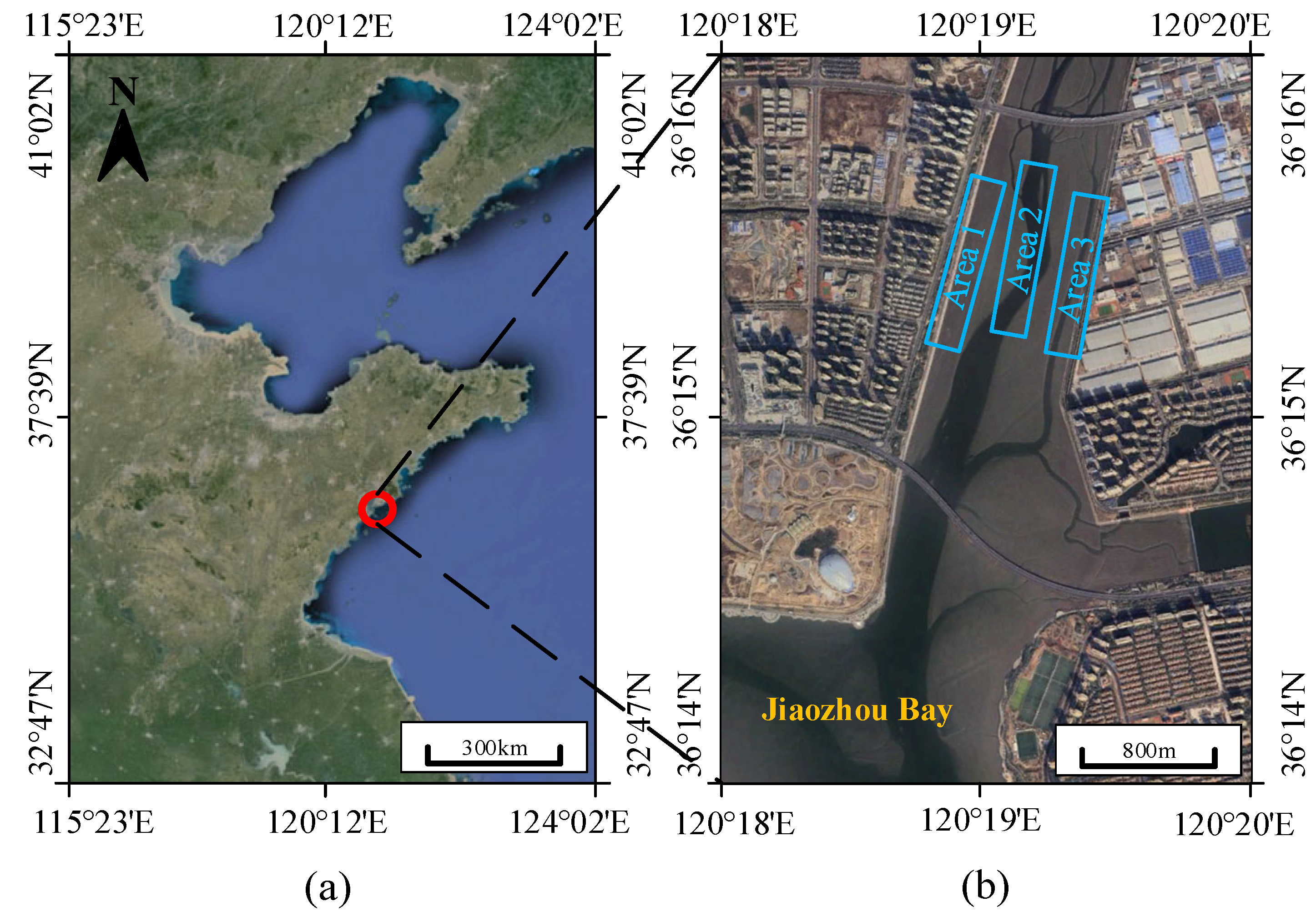
2.1. Study Area and Dataset

The study area is located at the estuary of the Moshui River in Chengyang District, Qingdao city, Shandong Province, China (as shown in Figure 1a). This area is located in the southern part of the Jiaodong Peninsula. The river spans a total length of 41.52 km and has a watershed area of 317.2 square kilometers, with rainfall concentrated between July and September each year. The upper reaches of the river have steep gradients and rapid water flow, leading to frequent changes in the riverbed. The western side of the Moshui River is a wetland park with abundant vegetation, while the eastern side is an industrial park in active use. During non-rainy seasons, the water flow in this area is minimal, and water is present only in the middle of the river channel, leaving large areas of the riverbed near the banks exposed. Consequently, the area features a rich variety of land cover types, including trees, lawns, marginal banks, and water wetlands. This study selected three representative sample areas for classified research (as shown in Figure 1b).

In June 2022, data acquisition for the study area was conducted via a DJI Zenmuse L1 LiDAR scanner(DJI, Shenzhen, China). The DJI Zenmuse L1 integrates laser radar, a mapping camera, and high-precision inertial navigation equipment. Laser scanner data acquisition was performed in single-echo mode with a pulse repetition rate of 240 kHz and in dual-echo mode with a pulse repetition rate of 480 kHz. The auxiliary camera simultaneously obtained the RGB information of the scanned target; in addition, the IMU update frequency is 200 Hz, and all the recording points were saved in the LAS file [39]. The data used in this experiment were acquired in single-echo mode with a flight altitude of 80 m. The total number of points in the three sample areas is 44.84 million, with a point cloud density of 112 points per square meter. The sample areas include five main categories: trees, lawns, marginal banks, ground, and water wetlands (see Figure 2). To improve the applicability of the model algorithm, only simple denoising was performed. The statistical outlier removal function in CloudCompare v2.13 software was used, combined with manual intervention to remove noise points, and then the CloudCompare v2.13 software was used to annotate the five categories point by point to produce sample data (see

Table 1. Statistics on the number of point clouds in each category.

Area	Tree	Lawn	Marginal Bank	Ground	Water Wetland
Area_1	1,508,987	765,610	16,206,559	1,901,110	0
Area_2	638,955	1,419,880	3,362,761	2,149,429	0
Area_3	0	0	13,455,119	0	3,440,744
All points 44,849,154	2,147,942	2,185,490	33,024,439	4,050,539	3,440,744
	(4.8%)	(4.9%)	(73.6%)	(9.0%)	(7.7%)

and Figure 3). The number of point clouds for the marginal bank was the largest, accounting for 73.6%; the number of point clouds for the lawn and trees was relatively small, accounting for 4.9% and 4.8%, respectively. Each point in the sample data contains three-dimensional coordinates (x, y, z), RGB values, echo intensity, and category labels.

2.2. Methods

Estuarine areas have complex land cover types, and accurate object classification cannot be performed using only the raw features of point cloud data. To enhance the learning ability of the layered structures of the PointNet++ model for identifying target features, this study presents a multifeature-assisted and multilayer fused neural network (MLF-PointNet++) for LiDAR-UAS point cloud classification in estuarine areas. The classification method is shown in Figure 4.

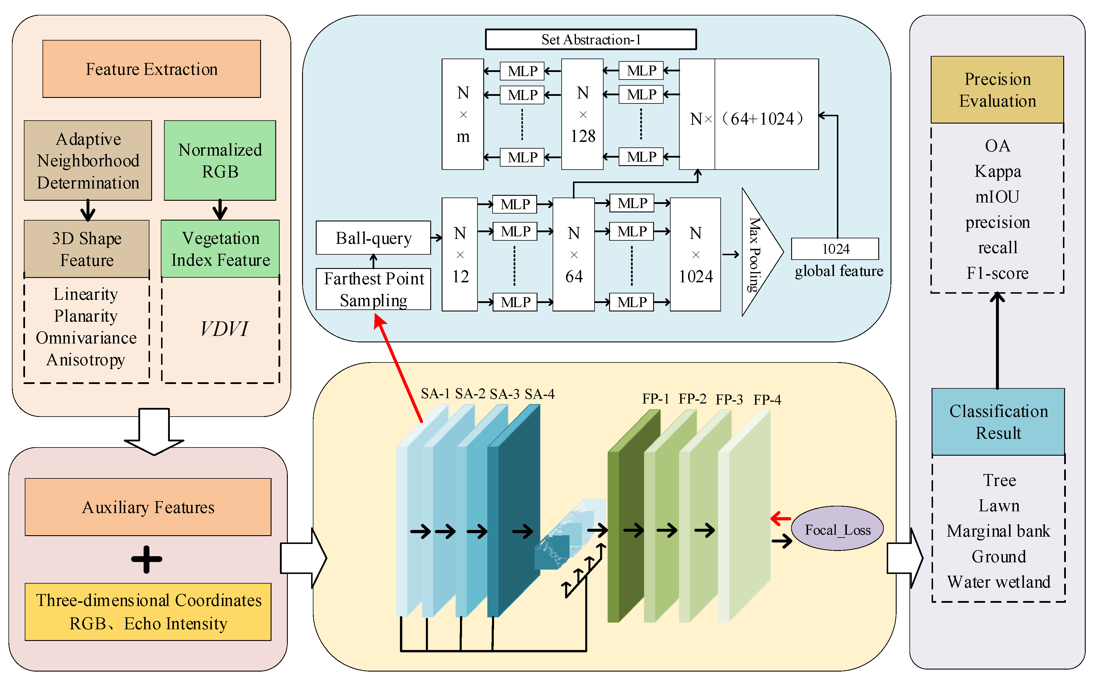
2.2.1. Feature Extraction

Owing to the lack of topological relationship information between points in point cloud data, directly extracting the shape and structure of objects from point cloud data is challenging. The incorporation of point cloud features or object feature descriptors can enhance the ability to recognize point cloud targets. For 3D shape features, linearity describes the linear distribution characteristics of point cloud data in a specific direction; planarity describes the flatness of the surface of the three-dimensional object represented by the point cloud; omnivariance measures the dispersion or fluctuation degree of the point cloud data; and anisotropy describes the degrees of variation in different directions of the point cloud, which is significant for understanding the shape and structure of three-dimensional objects. The visible-band difference vegetation index (VDVI) can reflect information about the growth conditions and coverage extent of green vegetation, which helps distinguish different types of vegetation in vegetation classification. Therefore, these features of the point cloud are used as auxiliary features.

(1)

Extraction of 3D shape features. Owing to the different scanning distances, scanning angles, and scanning target characteristics (discrete distributions of tree point clouds and uniform distributions of ground point clouds), the acquired point cloud data are nonuniform. To reduce the feature calculation errors caused by uneven point cloud density, a neighborhood adaptive method is adopted to calculate 3D shape features. To calculate the optimal neighborhood radius $r_{optimal}$ of a point, the principal component analysis method is first used to calculate the eigenvalues of the feature matrix composed of neighborhood point coordinates. The optimal neighborhood radius $r_{optimal}$ is determined by changing the radius parameter $r_{\Delta }$ and selecting the value that produces the minimum feature entropy. The 3D shape features are subsequently calculated via the eigenvalues ${\lambda }_1$, ${\lambda }_2$, and ${\lambda }_3$ (${\lambda }_1\ge {\lambda }_2\ge {\lambda }_3$) of the feature matrix composed of the point cloud coordinates in the optimal neighborhood. 3D shape features include linearity, planarity, scattering, omnivariance, anisotropy, eigenentropy, traces, and changes in curvature. Adding all the features increases the complexity of the model calculations. To improve the calculation efficiency of the algorithm, we use the random forest algorithm to analyze the importance of these 3D shape features. The first four 3D shape features with significant influence—linearity, planarity, omnivariance, and anisotropy—were selected as auxiliary features. The specific calculation formula can be found in reference [40].

(2)

Extraction of the VDVI. The dense vegetation (lawns and trees) on the slopes in the estuarine area has elevation and fitting residual information similar to the ground on the tops of the slopes. The vegetation on the slopes and the ground at the tops of the slopes may be mixed into one category during point cloud classification [41]. The vegetation index can effectively reflect the distribution of vegetation and help distinguish ground from vegetation. Because the same object often has similar or continuous RGB color information and because the color changes between different objects are significant, this article transforms the target RGB color information into the VDVI to highlight the differences between the vegetation and ground [41]. The calculation formula for the VDVI is as follows:

$$VDVI={\displaystyle \frac{2G-R-B}{2G+R+B}}$$

(1)

where R, G, and B denote the red, green, and blue color values of the target, respectively.

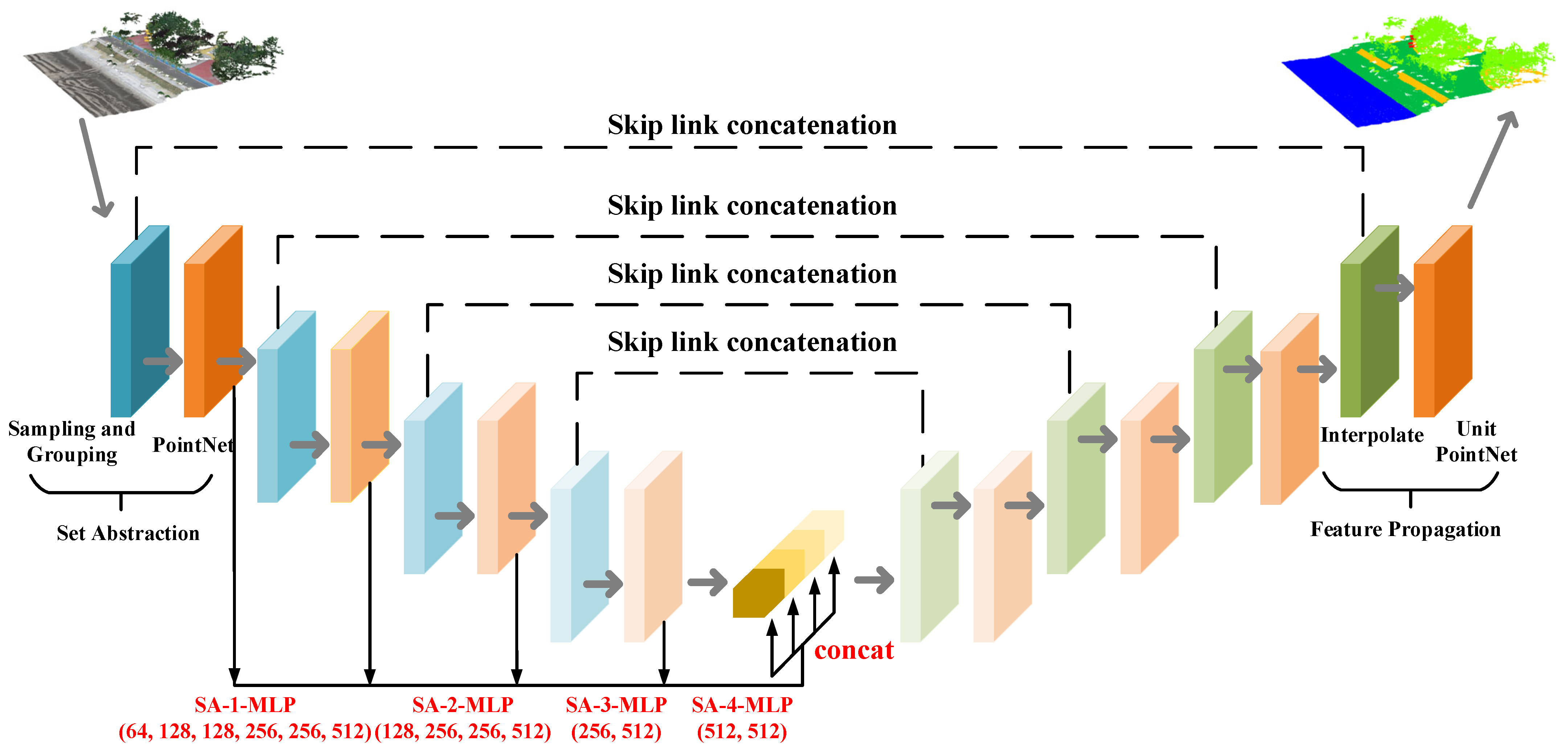
2.2.2. MLF-PointNet++ Model Construction

The MLF-PointNet++ model proposed in this article was developed on the basis of PointNet++ and is a deep neural network that can directly use unordered point cloud data. Because PointNet++ uses only the set abstraction of the last layer to extract feature vectors, low-level features are not considered, and some spatial information is lost. The MLF-PointNet++ proposed in this article integrates the feature vector output from multiple layers of set abstraction into a feature vector that integrates low-layer and high-layer information through MLP dimensionality enhancement, improving its fine-grained recognition and generalization abilities for complex scenes.

MLF-PointNet++ consists of four set abstractions and four feature propagations, and skip link concatenation is used in the U-Net architecture to enhance feature learning and information fusion between set abstractions and feature propagations. This not only helps alleviate gradient loss problems but also promotes information flow between different levels [42]. Each set abstraction consists of three parts: a sampling layer, a grouping layer, and a PointNet. In the sampling layer, a local center point is selected from the input LiDAR-UAS point cloud set $\{x_1,x_2\cdot \cdot \cdot x_n\}$, and farthest point sampling (FPS) is used to select a subset $\{x_{i1},x_{i2}\cdot \cdot \cdot x_{ij}\}$ from the input point cloud set. Each point in the subset is the farthest point from the remaining points. In the grouping layer, a point cloud set of size $N\times (d+C)$ is input, where $N$ is the number of points, $d$ is the coordinate dimension, and $C$ is the feature dimension of RGB, echo intensity, linearity, planarity, omnivariance, anisotropy, and VDVI. We select a center point of size $N_1\times d$, take each center point as the center in turn, and sample $K$ points in a sphere with a radius of $r$. A sphere query is used to divide the point cloud into $N_1$ local regions, thereby generating a point cloud set of size $N_1\times K\times (d+C)$. In the PointNet layer, $N_1$ local regions of size $K\times (d+C)$ are input. First, the MLP is used to perform dimensionality enhancement on each local region of the data, a $K\times 1024$-dimensional point cloud feature matrix is generated, max pooling is used for local feature extraction, and then the global and local features of the point cloud are combined. As the input for the next set abstraction step, the combined feature vector is fused with the feature vector output by the previous set abstraction step through MLP dimensionality enhancement, forming a combined feature vector containing both low-layer and high-layer information. Each set abstraction step performs the same operation (as shown in Figure 5), and the fusion forms the final combined feature vector. Finally, the combined feature vectors are fed into a feature propagation layer composed of interpolation layers and a unit PointNet. In each feature propagation step, the inverse distance weight (IDW) method is used to interpolate the point features onto the target point. Shallow-layer features are calculated on the basis of the deep-layer features of each point in the current network. Jump connections are used to fuse the interpolated features with the output features of the corresponding set abstraction, which are then input into PointNet to obtain new features. After upsampling through four layers of feature propagation, the final classification result for each point can be obtained, thus completing point cloud classification of the estuarine area.

2.2.3. Focus Loss Function

Owing to the uneven number of point clouds for various ground targets scanned by LiDAR-UAS in estuarine areas, the numbers of point clouds for trees, lawns, marginal banks, ground, and water wetlands account for 4.8%, 4.9%, 73.6%, 9.0%, and 7.7%, respectively, of the total number of point clouds. There is a significant difference in the number of point clouds among the different categories. During sampling, categories with a high number and density of point clouds are prone to oversampling, while categories with a low number and density of point clouds are prone to undersampling, resulting in varying degrees of overfitting in the model and affecting the accuracy of training. To address the impact of the uneven number of point clouds across different categories on model classification, a focus loss function is introduced for model optimization [43].

The focus loss function is developed from the cross-entropy function, which closely monitors the classification of smaller categories by resetting weights. The traditional binary cross-entropy loss function $CE(p_t)$ is as follows:

$$CE(p_t)=-\log (p_t)$$

(2)

where $p_t$ is the estimated probability of the model for the category; please refer to [43] for details. To solve the problem of imbalanced numbers of point clouds across categories, a weighting factor $\alpha \in [0,1]$ is introduced for Category 1, and a weighting factor $1-\alpha$ is introduced for Category −1. In practice, $\alpha$ can be set by the inverse frequency or as a hyperparameter through cross-validation. For the convenience of labeling, the category weight coefficient ${\alpha }_t$ is defined as:

$${\alpha }_t=\{\begin{array}{cc}\alpha & \begin{array}{cc}if& y=1\end{array}\\ 1-\alpha & otherwise\end{array}$$

(3)

We multiply Formula (3) by Formula (2) to obtain:

$$CE(p_t)=-{\alpha }_t\log (p_t)$$

(4)

The category weight coefficient ${\alpha }_t$ is a fixed value and can be considered a hyperparameter. Although ${\alpha }_t$ can balance the importance of positive and negative values to solve the problem of class imbalance, distinguishing between samples that are easy and difficult to recognize remains challenging. Therefore, a modulation factor ${(1-p_t)}^{\gamma }$ is set in Formula (4) to achieve greater numerical stability. The formula for calculating the focal loss function $FL(p_t)$ is as follows:

$$FL(p_t)=-{\alpha }_t{(1-p_t)}^{\gamma }\log (p_t)$$

(5)

where $\gamma$ is the focusing parameter, used to adjust the rate at which the weights of easily recognized categories are reduced. Since the number of marginal bank point clouds in these experimental data is large, it affects the classification accuracy of other categories during model training. Therefore, this study uses the focal loss function as the loss function in the MLF-PointNet++ model. The proportion of the marginal bank is set to ${\alpha }_t$, and the other categories are set to $1-{\alpha }_t$. By reducing the weight of easily identifiable samples and increasing the weight of difficult-to-identify samples and samples with fewer category points, the MLF-PointNet++ model training is optimized.

3. Results

3.1. Experimental Parameter Settings

All the experiments are conducted on a computer with an NVIDIA GeForce RTX 3060 Ti GPU(Santa Clara, CA, USA) and Intel Core i9-12900H CPU(Santa Clara, CA, USA). All the programs are implemented via the Windows 11 system and Python 3.7, and the networks are constructed via PyTorch 1.7.0. On the basis of existing backpropagation algorithms, the Adam algorithm is used to optimize the network parameters. When extracting point cloud features, the optimal neighborhood radius and parameter settings for calculating the 3D shape features are $r_{\min }$ = 0.5, $r_{\max }$ = 8.0, and $r_{\Delta }$ = 0.5; the number of sampling points is set to 2048; the batch size is set to 16; the number of epochs is set to 32; and the learning rate is set to 0.001 during model training. In the focus loss function, ${\alpha }_t$ = 0.2 and $\gamma$ = 2. Each of the three selected representative sample areas was divided into 10 small sample area blocks on average. Seventy percent of the data from each representative area were selected as the training set, and K-fold cross-validation was used to train and validate the model. The other 30% of the data were used as the test set to test the effectiveness of the model in this area. Comparative experiments were also conducted with random forest and PointNet++ models.

Using manual point cloud labels as a reference, the classification accuracy of objects in estuarine areas scanned by LiDAR-UAS was quantitatively analyzed via the following evaluation metrics: confusion matrix, overall accuracy (OA), mean intersection over union (mIOU), kappa coefficient, precision, recall, and F₁-score. To comprehensively analyze the classification results of objects in the estuarine area, the following formulas were used to calculate the evaluation index, and the average values of the evaluation index across all areas were used to evaluate the classification effect. The formulas for these metrics are as follows:

$$OA={\displaystyle \frac{tp+tn}{tp+tn+fp+fn}}$$

(6)

$$mIOU={\displaystyle \frac{tp}{tp+fp+fn}}$$

(7)

$$p_e={\displaystyle \frac{(tp+fn)\times (tp+fp)}{{(tp+tn+fp+fn)}^2}}+{\displaystyle \frac{(tn+fp)\times (tn+fn)}{{(tp+tn+fp+fn)}^2}}$$

(8)

$$Kappa={\displaystyle \frac{OA-p_e}{1-p_e}}$$

(9)

$$precision={\displaystyle \frac{tp}{tp+fp}}$$

(10)

$$recall={\displaystyle \frac{tp}{tp+fn}}$$

(11)

$$F_1-score=2\times {\displaystyle \frac{precision\times recall}{precision+recall}}$$

(12)

where $tp$ is the number of positive samples correctly identified as positive, $tn$ is the number of negative samples correctly identified as negative, $fp$ is the number of negative samples incorrectly identified as positive, and $fn$ is the number of positive samples incorrectly identified as negative.

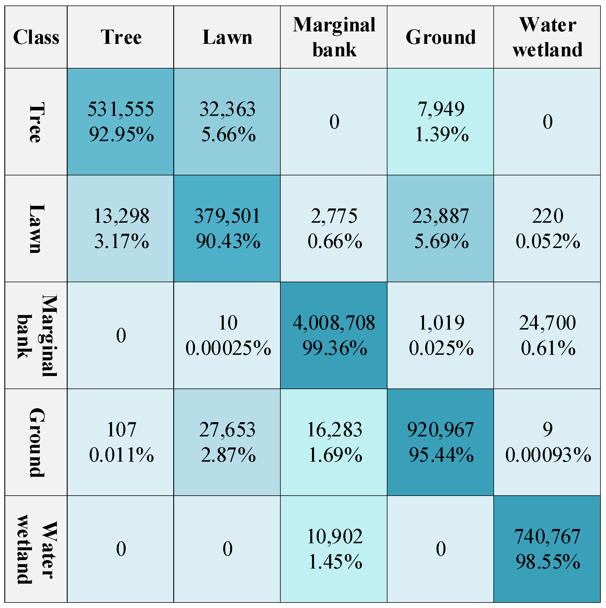
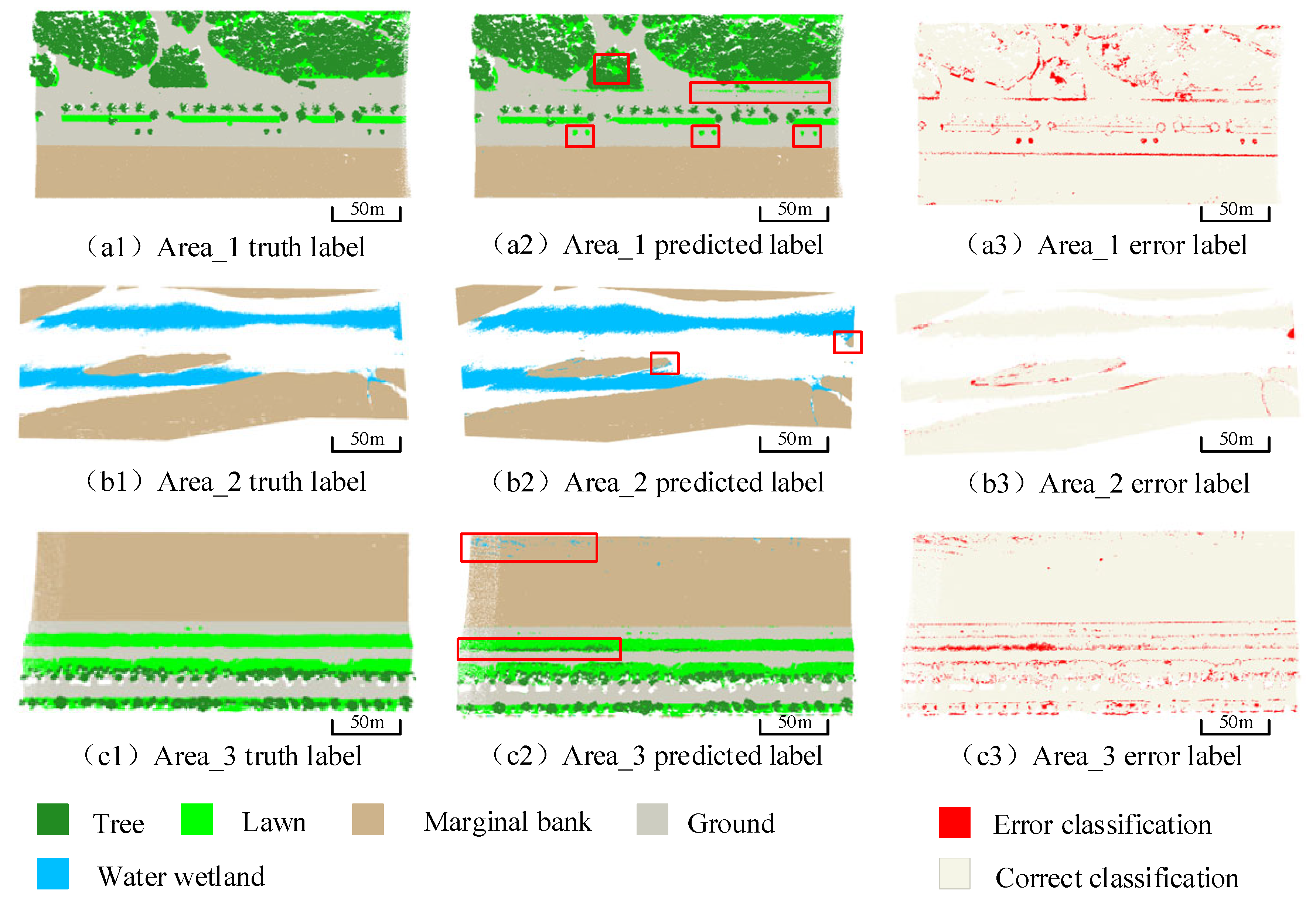
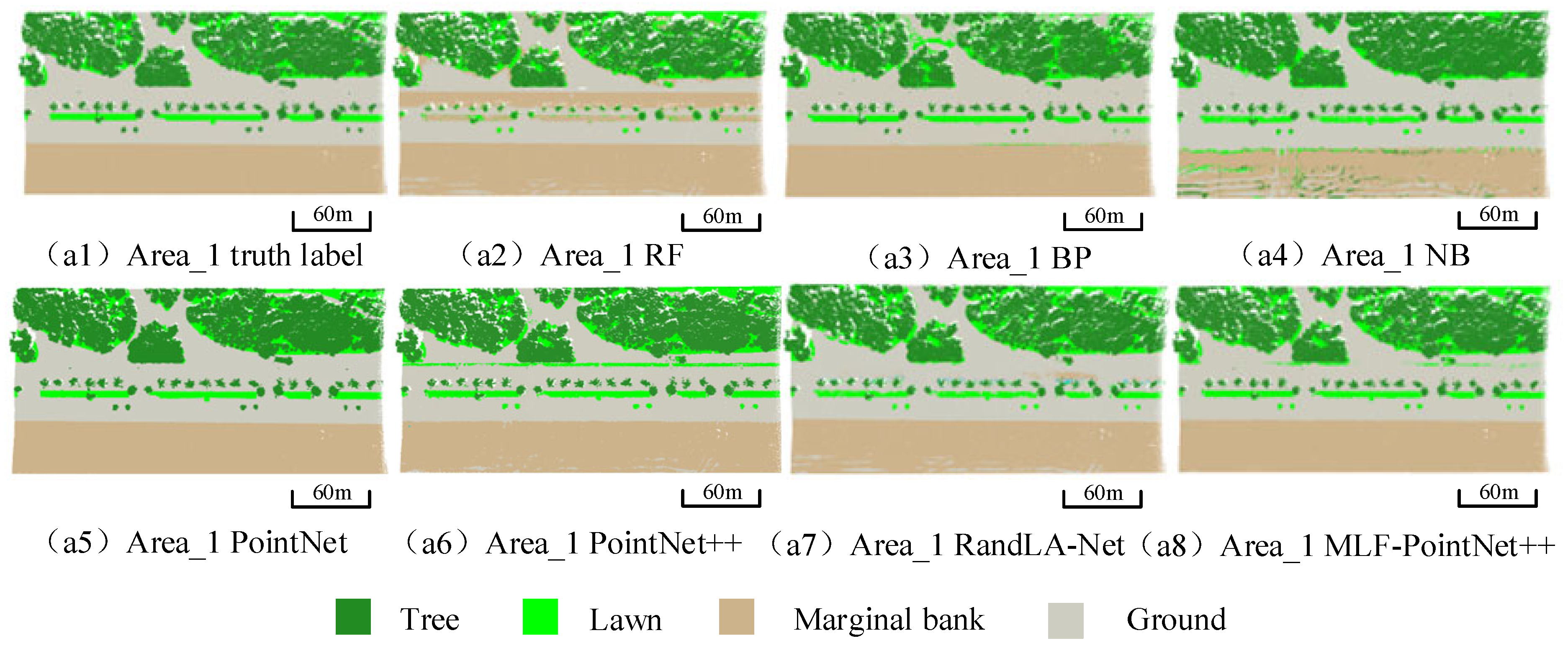
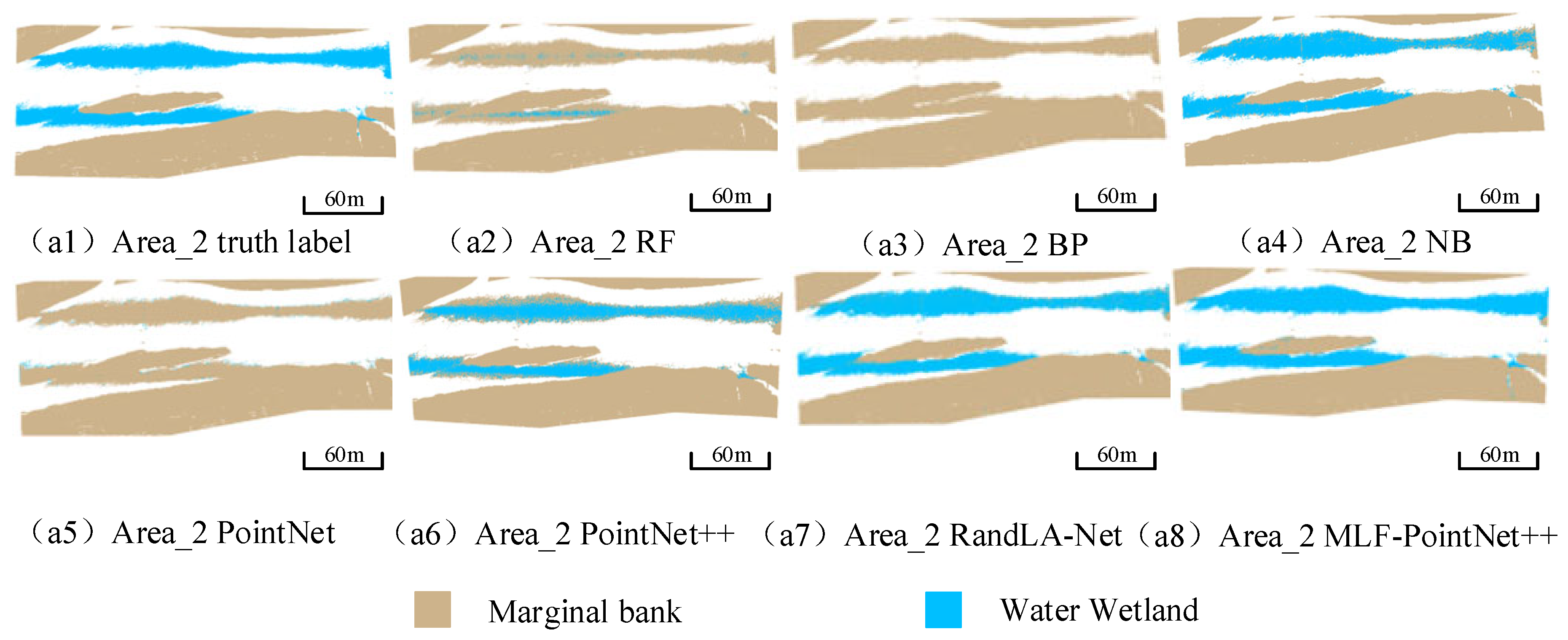
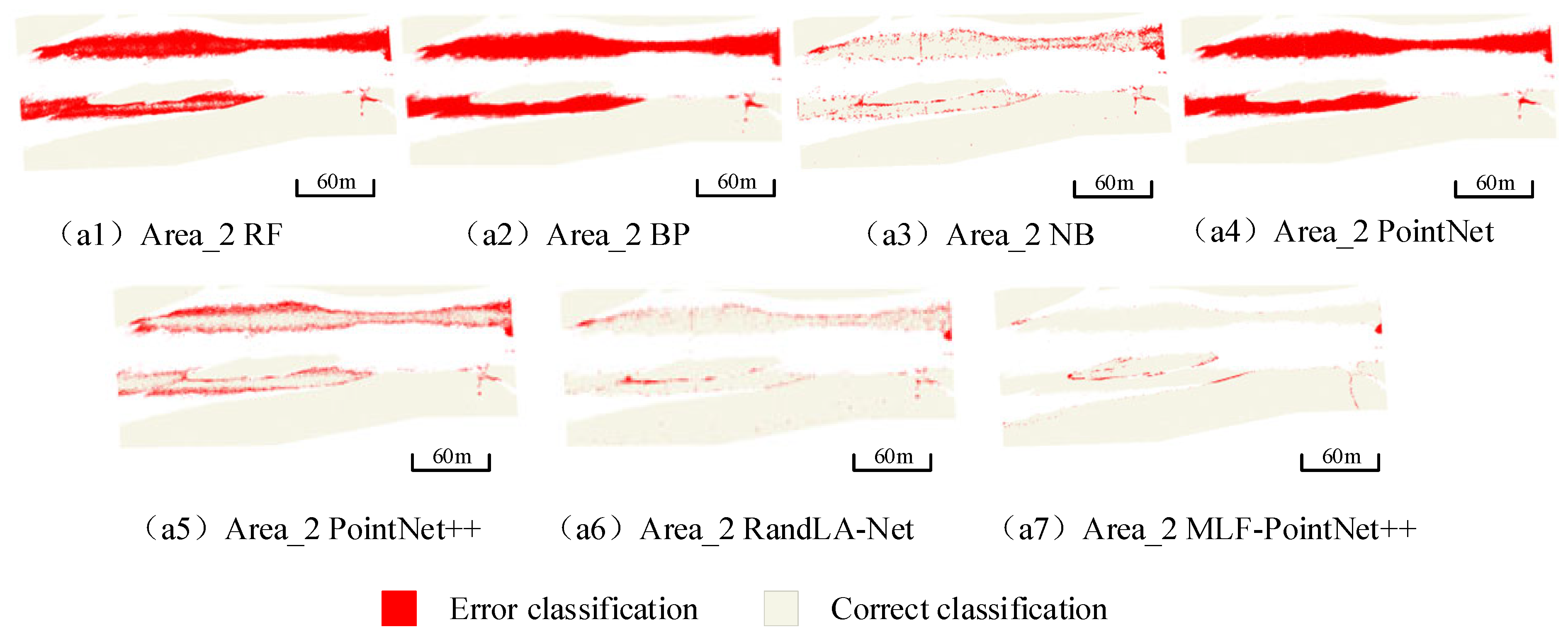
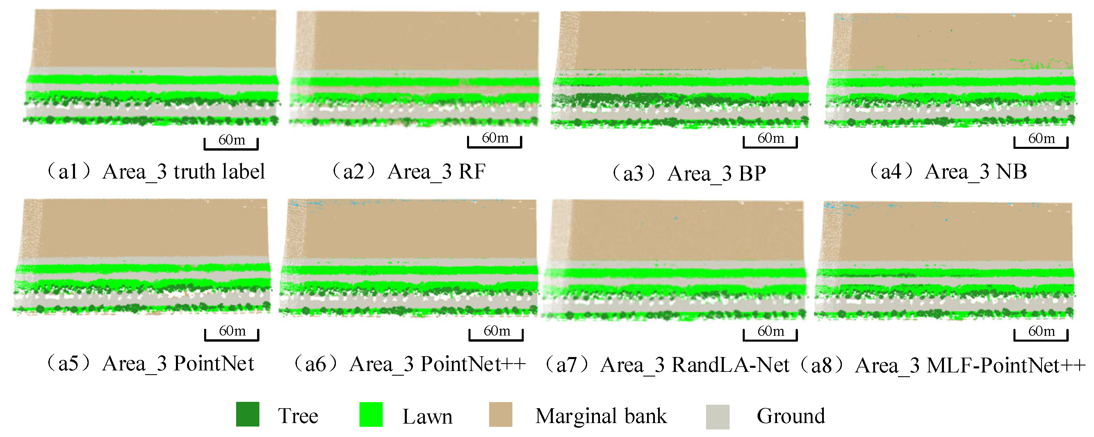
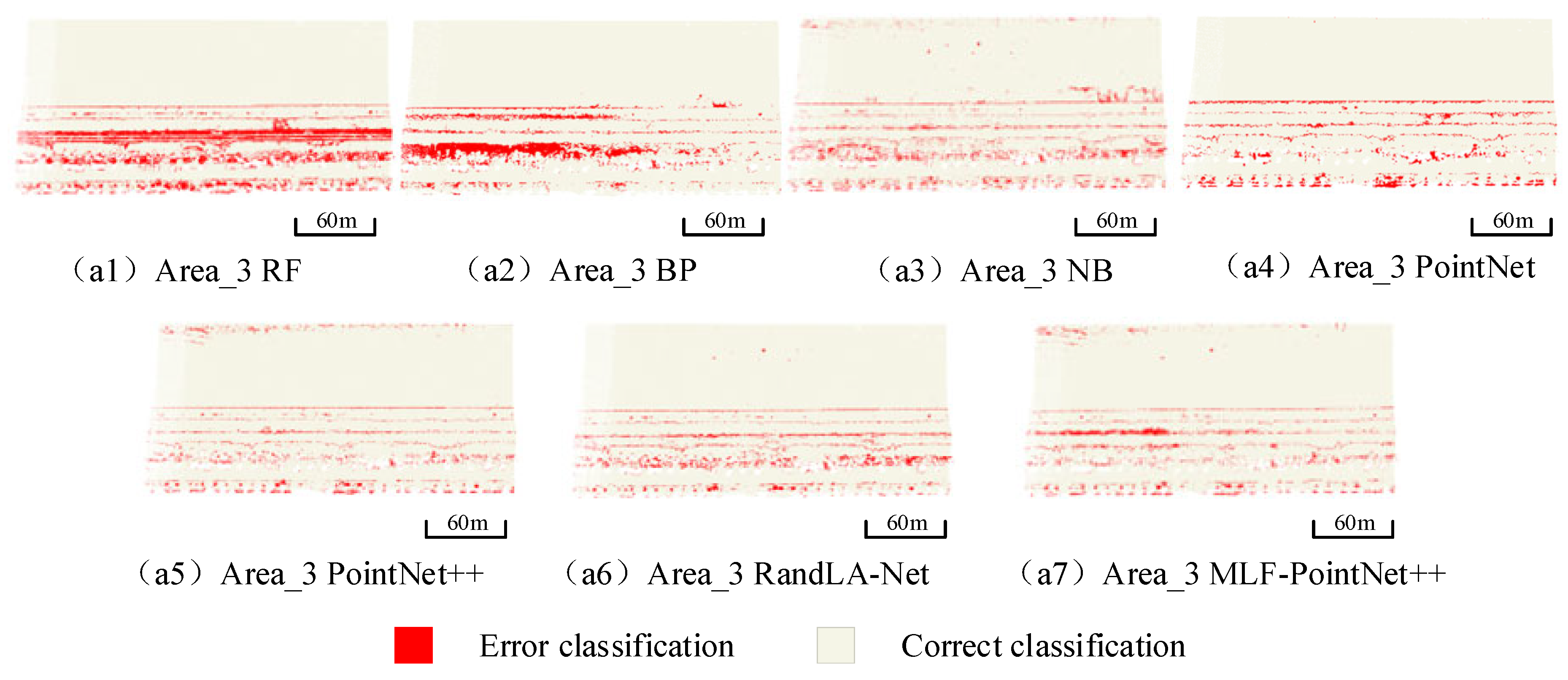
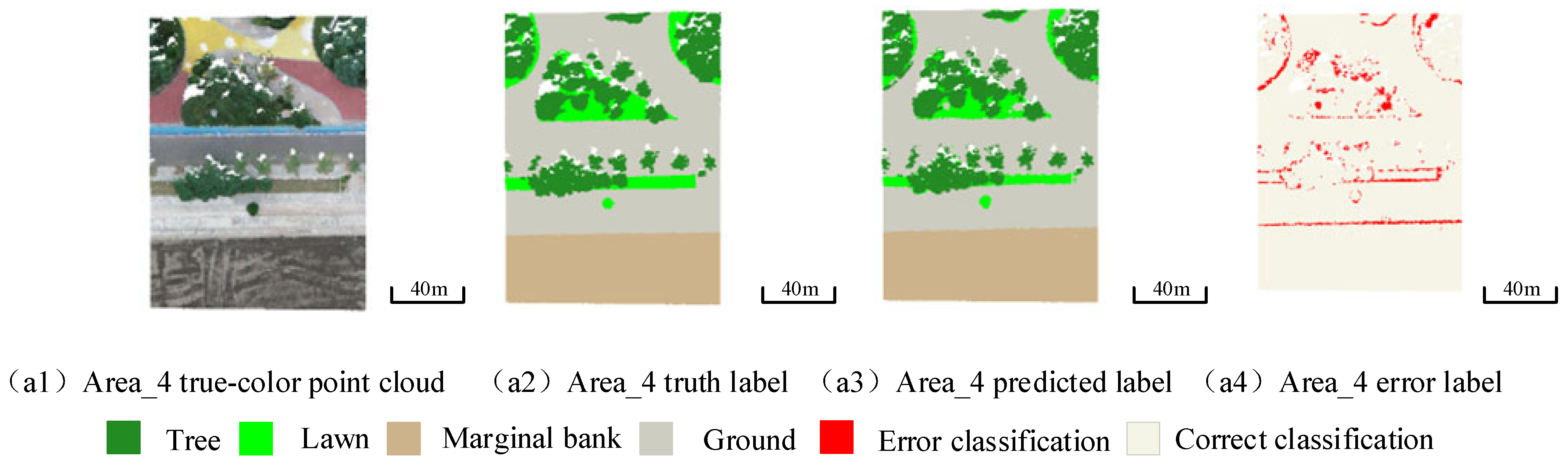
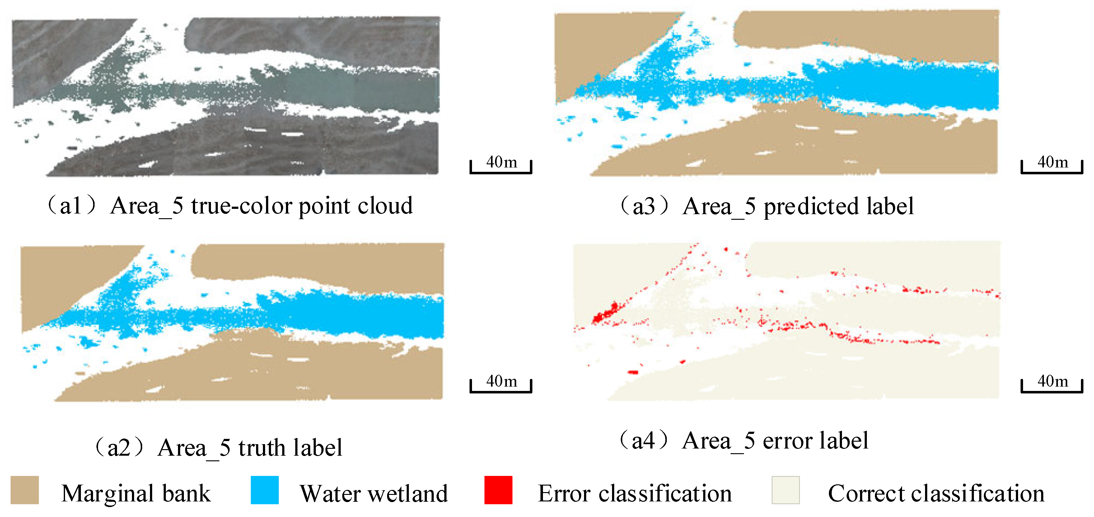
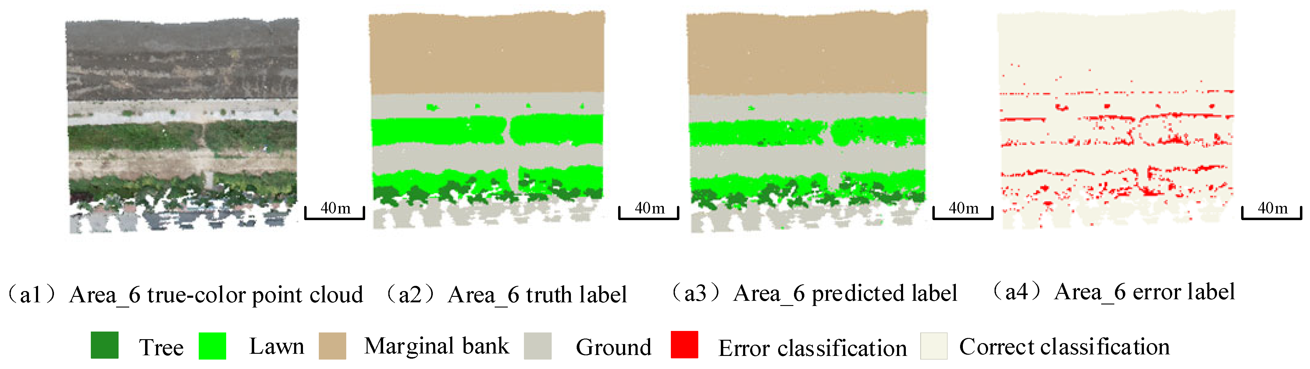
3.2. Experimental Results

This study uses three-dimensional coordinates (x, y, z), RGB, echo intensity, linearity, planarity, omnivariance, anisotropy, VDVI, and category labels as model inputs for classification via the MLF-PointNet++ model. The accuracy of each indicator in the experimental results is the average of the prediction results across three areas. The results revealed that the mean OA, mIOU, kappa coefficient, precision, recall, and F₁-score across the three representative areas were 0.976, 0.912, 0.960, 0.953, 0.953, and 0.953, respectively. The precision for the tree, lawn, marginal bank, ground, and water wetland categories was 0.930, 0.904, 0.994, 0.954, and 0.986, respectively. As shown in the confusion matrix (Figure 6), 1.39% of the tree points were misclassified as ground points, 5.66% of the tree points were misclassified as lawn points, 5.69% of the lawn points were misclassified as ground points, 3.17% of the lawn points were misclassified as tree points, 0.61% of the marginal bank points were misclassified as water wetland points, 1.69% of the ground points were misclassified as marginal bank points, 2.87% of the ground points were misclassified as lawn points, and 1.45% of the water wetland points were misclassified as marginal bank points. Although there is some misclassification, the precision for each category is above 0.900. Among these categories, the precision for the marginal bank and water wetland areas is the highest, and the overall classification effect is good.

Further analysis of the misclassification of point clouds (as shown in Figure 7) reveals that in the vegetation area of Area 1, owing to the flourishing growth of weeds, the elevation is similar to that of low trees, resulting in the misclassification of lawn points as tree points. The classification between the marginal bank and the ground is good, but some ground points in the red-boxed area are mistakenly classified as lawn points. This is because there is a colored plastic runway on the ground in Area 1. The echo intensities of the lawn and plastic ramp on the ground are relatively close, and the difference in elevation is small, making it difficult to accurately distinguish between ground points and lawn points in terms of RGB, echo intensity, and elevation features. Since there are only two categories of target information in Area 2, the overall classification performance is optimal. However, there is still a small amount of misclassification at the intersection of water wetlands and marginal banks, which is due to the similar echo intensities. Owing to significant elevation differences near the riverbank slopes in Area 3, some lawn points on the riverbank slopes were mistakenly classified as tree points. Owing to their proximity to the water wetland in the middle water area and similar geographical distribution, some of the marginal bank points were misclassified as water wetland points. Some of the marginal banks in Area 3 were misclassified as water wetland points because of their proximity to the intermediate water wetland and similar geographical distributions. The elevation difference near the estuarine bank slope was large, resulting in some lawn points on the bank slope being misclassified as tree points. Although the focal loss function can improve the precision of lawns, the number of point clouds of trees and lawns is the smallest, and the effective features extracted during model training are not comprehensive, the precision is still relatively low across all categories. In addition, the experiments revealed that most of the point cloud misclassification phenomena occur at the junction of categories. At the junction of the marginal bank, ground and water wetland, point cloud characteristics such as elevation information do not change significantly, and the points on the surfaces of each category are closely mixed, making it difficult for the MLF-PointNet++ model to capture small structural changes, causing errors when extracting point cloud neighborhood features. This makes it impossible to accurately distinguish the point cloud information at the junction.

The MLF-PointNet++ method is compared with random forest, BP neural network, Naive Bayes, PointNet, PointNet++, and RandLA-Net.

Table 2. Comparative experimental evaluation of seven different training models.

Model	OA	mIOU	Kappa	Precision	Recall	F1-Score
RF	0.843	0.641	0.706	0.711	0.909	0.755
BP	0.857	0.642	0.737	0.722	0.703	0.710
NB	0.949	0.837	0.917	0.912	0.904	0.907
PointNet	0.863	0.675	0.747	0.744	0.905	0.733
PointNet++	0.956	0.870	0.924	0.919	0.944	0.929
RandLA-Net	0.969	0.900	0.948	0.942	0.952	0.946
MLF-PointNet++	0.976	0.912	0.960	0.953	0.953	0.953

lists the results of the classification experiment comparing MLF-PointNet++ with random forest, BP neural network, Naive Bayes, PointNet, PointNet++, and RandLA-Net in estuarine areas. The experimental results show that the accuracy of the random forest model in machine learning is the lowest, with an overall accuracy (OA) of 0.843, and the BP neural network is close to the random forest. There are apparent misclassifications between the ground and the marginal bank in the random forest results in Area 1 (as shown in Figure 8 and Figure 9). It is difficult for the random forest and BP neural network methods to accurately distinguish the water wetland and the marginal bank in Area 2 (as shown in Figure 10 and Figure 11). The precision of the BP neural network in classifying trees is 0.945, showing its advantages. The results of the Naive Bayes method are better than those of the other two methods in machine learning. Although the Naive Bayes method accurately classifies the water wetland and the marginal bank in Area 2 (as shown in

Table 3. Classification accuracy of different training models for different categories.

Model	RF	BP	NB	PointNet	PointNet++	RandLA-Net	MLF-PointNet++
Tree	0.799	0.945	0.944	0.895	0.927	0.903	0.930
Lawn	0.819	0.729	0.752	0.886	0.935	0.939	0.904
Marginal bank	0.998	0.999	0.972	0.999	0.995	0.996	0.994
Ground	0.722	0.935	0.954	0.932	0.935	0.922	0.954
Water wetland	0.220	0.000	0.939	0.008	0.806	0.952	0.986

), it misclassifies the marginal bank in Areas 1 and 3 as lawn and tree (as shown in Figure 8, Figure 9, Figure 12 and Figure 13).

In deep learning models, the PointNet model does not fully utilize metric space distance to extract local features, resulting in low classification accuracy and difficulty in identifying the water wetland and marginal bank in Area 2 (as shown in Figure 9 and Figure 12). PointNet++ uses a hierarchical structure to extract local information from points and achieves an overall accuracy (OA) of 0.956. The precision for water wetland and marginal bank in Area 2 is 0.806 and 0.995 respectively. The overall accuracy (OA) of the RandLA-Net model is 0.969. The RandLA-Net model uses a local feature aggregation module to extract point cloud features with random sampling. Thus, the uneven density of point clouds may affect classification accuracy. For the classification of the MLF-PointNet++ model, the precision for each category is above 0.900, especially the precision for ground and water wetland, which is 0.954 and 0.986 respectively. For the results of MLF-PointNet++ in Area 1, the ground points and lawn points can be accurately distinguished. The proposed multi-layer feature fusion enhances the effect of the MLF-PointNet++ model on point cloud feature extraction. The edge points of the water wetland in Area 2 can also be accurately distinguished, and the precision of the water wetland has reached 0.986. The misclassification error of category boundaries in Area 3 is smaller than that of PointNet++ and RandLA-Net. Therefore, the MLF-PointNet++ model is better than other models in classifying objects scanned by LiDAR-UAS in the estuarine area.

To further verify the classification performance of the MLF-PointNet++ model, this paper selects three areas that did not participate in training and testing for verification analysis. The model inputs for the experiment are three-dimensional coordinates (x, y, z), RGB values, echo intensity, linearity, planarity, omnivariance, anisotropy, VDVI, and category labels. The MLF-PointNet++ model is used to classify these three newly added areas. The results show that the overall accuracy (OA), mean intersection over union (mIOU), Kappa coefficient, precision, recall, and F₁-score for the three newly added areas 4, 5, and 6, are 0.959, 0.901, 0.940, 0.943, 0.951, and 0.946, respectively. The precision for tree, lawn, marginal bank, ground, and water wetland is 0.993, 0.970, 0.948, 0.813, and 0.992, respectively. In Areas 4, 5, and 6, each category is accurately classified. Misclassification phenomena are mainly concentrated at the junctions between categories. In Area 4, there are more misclassifications at the junction between the ground and the lawn (as shown in Figure 14). In Area 5, there are still a few misclassifications at the junction between the water wetland and the marginal bank (as shown in Figure 15). In Area 6, due to the large number of weeds and their scattered distribution, part of the lawn was misclassified as ground (as shown in Figure 16). Overall, there are fewer misclassified points in each category across the three areas, so for untrained areas, this is consistent with the results of the previous classification tests of the proposed method, further verifying the effectiveness of the proposed method in the classification of objects in estuarine areas.

4. Discussion

To analyze the effectiveness of auxiliary features and the focal loss function on classification, ablation experiments of these two factors were designed in this study. By analyzing the results of these ablation experiments, we demonstrate the impact of auxiliary features and the loss function on the classification results. Then, the impact of the number of epochs on the performance of MLF-PointNet++ is analyzed, and the applicability and application scalability of the model is discussed.

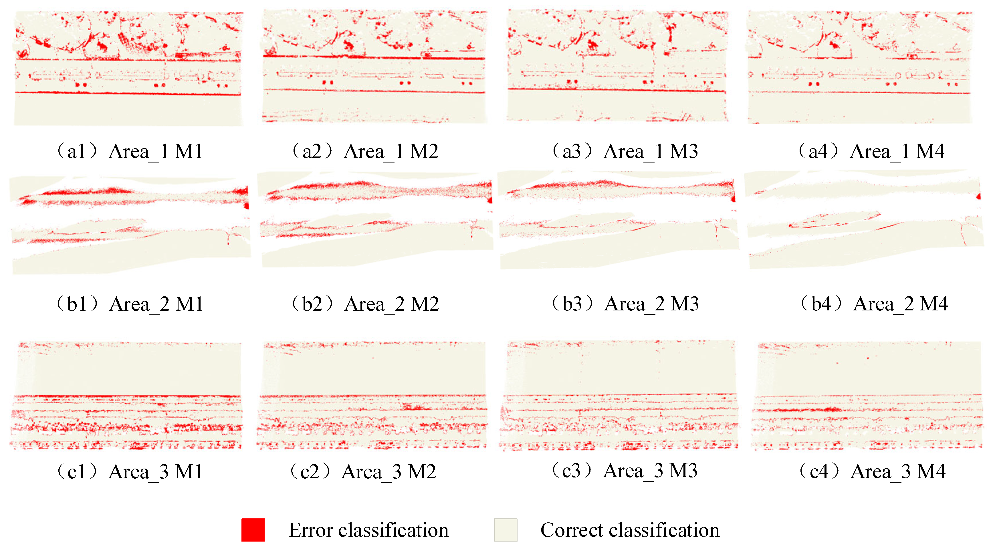
4.1. Auxiliary Feature Ablation Experiment

To verify the effectiveness of auxiliary features for object classification in estuarine areas via LiDAR-UAS, MLF-PointNet++ was used as the training model. The model inputs were as follows: (1) three-dimensional coordinates (x, y, z), RGB, and echo intensity (M1); (2) three-dimensional coordinates (x, y, z), RGB, echo intensity, and VDVI (M2); (3) three-dimensional coordinates (x, y, z), RGB, echo intensity, linearity, planarity, omnivariance, and anisotropy (M3); and (4) three-dimensional coordinates (x, y, z), RGB, echo intensity, linearity, planarity, omnivariance, anisotropy, and VDVI (M4). The ablation experiments were conducted in the experimental environment described in Section 3.1, and the other parameters remained unchanged.

Table 4. Evaluation indicators for the auxiliary feature ablation experiments.

Test	OA	mIOU	Kappa	Precision	Recall	F1-Score
M1	0.948	0.845	0.910	0.901	0.932	0.913
M2	0.958	0.866	0.929	0.918	0.937	0.926
M3	0.965	0.887	0.941	0.932	0.947	0.939
M4	0.976	0.912	0.960	0.953	0.953	0.953

lists the evaluation metric results for the classification of objects in estuarine areas via LiDAR-UAS scans from the four ablation experiment groups. Compared with the values obtained with M1, M4 improved the OA, mIOU, kappa coefficient, precision, recall, and F₁-score by 2.8%, 6.7%, 5.2%, 2.1%, and 4.0%, respectively; M3 improved them by 1.7%, 4.2%, 3.1%, 3.1%, 1.5%, and 2.6%, respectively; and M2 improved them by 1.0%, 2.1%, 1.9%, 1.7%, 0.5%, and 1.3%, respectively. After all auxiliary features were added, the classification accuracy of each category was better than that achieved using only the original features (see Table 4). There are differences of 0.7%, 2.1%, 1.2%, 1.4%, 1.0%, and 1.3% in the OA, mIOU, Kappa coefficient, precision, recall, and F₁-score, respectively, between M2 and M3. On the basis of the original features, both the 3D shape features and VDVI improved classification accuracy to varying degrees, with 3D shape features having a more significant impact on the classification results of objects in estuarine areas via LiDAR-UAS scans than VDVI. For M4, misclassification at the intersection of the marginal bank and the ground in Area 1 improved, and the boundary classification effect between the ground, tree, and lawn also increased. The classification performance for the water wetland and marginal bank in Area 2 significantly improved, and the misclassification of water wetlands as a marginal bank significantly decreased (as shown in Figure 17). These findings indicate that using 3D shape features and VDVI as auxiliary features effectively improves the ability to accurately distinguish objects in estuarine areas.

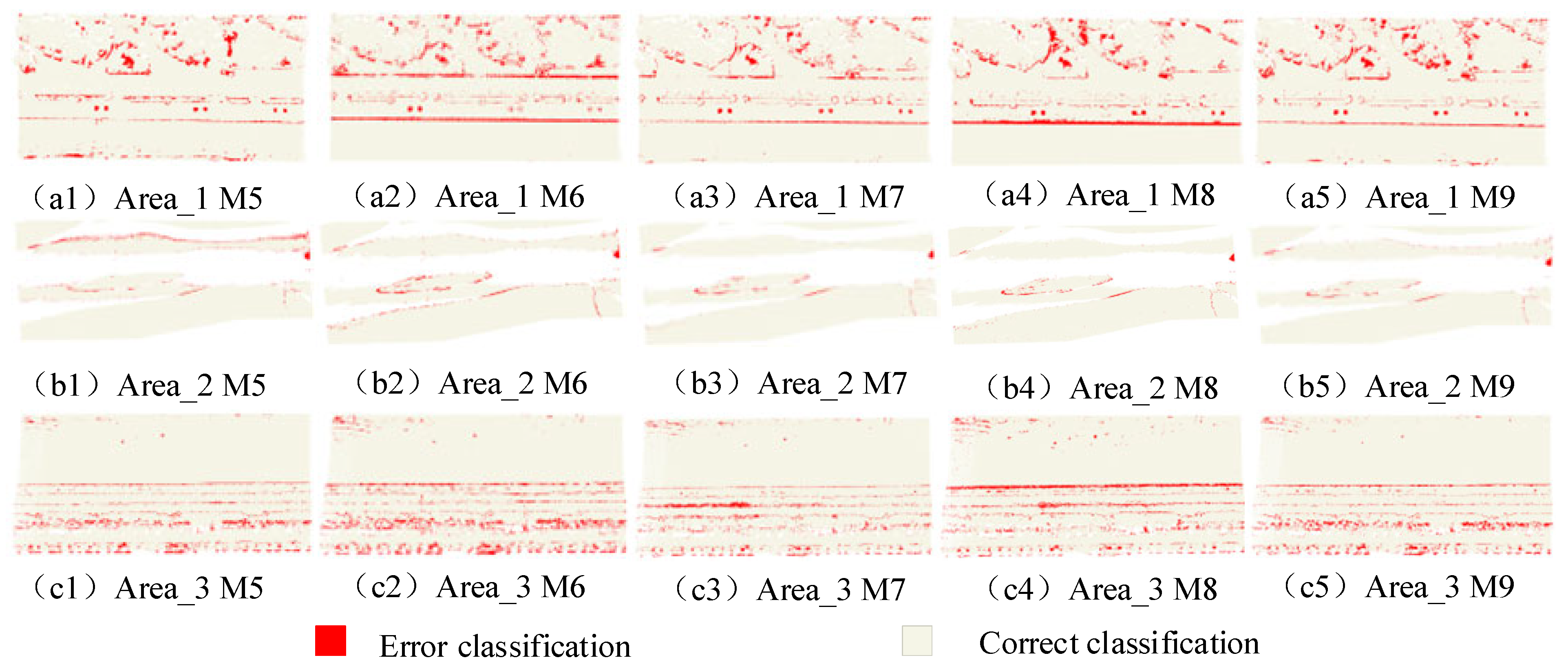
4.2. Loss Function Ablation Experiment

To validate the impact of the focal loss function on the classification accuracy of objects in estuarine areas via LiDAR-UAS scans, three-dimensional coordinates (x, y, z), RGB, echo intensity, 3D shape features, and VDVI were used as inputs to the model. The MLF-PointNet++ model was used as the training model, with the loss functions set as follows: (1) negative log likelihood loss (NLL_Loss) (M5); (2) focus loss function, where ${\alpha }_t$ = 0.15 (M6); (3) focus loss function, where ${\alpha }_t$ = 0.2 (M7); (4) focus loss function, where ${\alpha }_t$ = 0.25 (M8); and (5) focus loss function, where ${\alpha }_t$ = 0.3 (M9). The ablation experiments were conducted under the experimental environment described in Section 3.1, with all other parameters unchanged.

Table 5. Evaluation indicators for the loss function ablation experiments.

Test	OA	mIOU	Kappa	Precision	Recall	F1-Score
M5	0.972	0.898	0.953	0.940	0.951	0.944
M6	0.963	0.878	0.937	0.931	0.937	0.933
M7	0.976	0.913	0.960	0.953	0.953	0.953
M8	0.970	0.904	0.950	0.951	0.950	0.948
M9	0.971	0.897	0.951	0.941	0.949	0.944

lists the evaluation metric results for the classification of objects in estuarine areas via LiDAR-UAS scans from the five ablation experiment groups. The results indicate that M7 had the best classification performance. Compared with M5, M7 improved the OA, mIOU, kappa coefficient, precision, recall, and F₁-score by 0.4%, 1.5%, 0.7%, 1.3%, 0.2%, and 0.9%, respectively. The focus loss function performed better than the negative logarithmic likelihood function on the classification of objects scanned by LiDAR-UAS in estuarine areas and reduced the impact of the uneven number of point clouds in each category on the classification accuracy. The results of experiments M6, M7, M8, and M9 show the impact of the focal loss function on the classification of objects in the estuarine area under different class weight coefficients ${\alpha }_t$. Experiment M7 (${\alpha }_t$ = 0.2) is better than the classification results of experiments M6 (${\alpha }_t$ = 0.15), M8 (${\alpha }_t$ = 0.25), and M9 (${\alpha }_t$ = 0.3), and the experimental result of M6 (${\alpha }_t$ = 0.15) is the worst. The evaluation indicators for the classification results of M8 (${\alpha }_t$ = 0.25) and M9 (${\alpha }_t$ = 0.3) were relatively close. Setting the class weight coefficient too small or too large will lead to a decrease in classification accuracy, making classes with many point clouds lose their advantages. The setting of parameter ${\alpha }_t$ affects the classification accuracy of objects scanned by LiDAR-UAS in estuarine areas. Setting an appropriate parameter ${\alpha }_t$ can improve the classification accuracy for each category and reduce the misclassification of point clouds at the intersection of each category (as shown in Figure 18).

4.3. Epoch Discussion Experiment

To analyze the impact of epoch settings on the classification accuracy of the MLF-PointNet++ model, the epochs are set to: (1) epoch = 16 (M10); (2) epoch = 32 (M11); (3) epoch = 64 (M12). The three-dimensional coordinates (x, y, z), RGB color, echo intensity, linearity, planarity, omnivariance, anisotropy, and VDVI are used as input features. The experiments were all carried out in the experimental environment described in Section 3.1, with all other parameters unchanged.

Table 6. Comparative experimental evaluation of three different epochs.

Epoch	OA	mIOU	Kappa	Precision	Recall	F1-Score
M10(16)	0.9727	0.8910	0.9543	0.9384	0.9416	0.9393
M11(32)	0.9761	0.9125	0.9600	0.9534	0.9529	0.9529
M12(64)	0.9764	0.9136	0.9606	0.9543	0.9533	0.9536

lists the results of three sets of comparative experiments with epoch = 16, epoch = 32, and epoch = 64 on the classification of LiDAR-UAS scanning objects in estuarine areas. The results show that classification accuracy was highest when epoch = 64, with OA = 0.9764, mIOU = 0.9136, Kappa = 0.9606, precision = 0.9543, recall = 0.9533, and F₁-score = 0.9536. Compared with epoch = 32, classification accuracy at epoch = 64 improved by 0.0003, 0.0011, 0.0006, 0.0009, 0.0004, and 0.0007, respectively. However, the training time is twice that of epoch = 32. Classification accuracy was lowest at epoch = 16, with OA = 0.9727, mIOU = 0.8910, Kappa = 0.9543, precision = 0.9384, recall = 0.9416, and F₁-score = 0.9393. Compared with epoch = 16, classification accuracy at epoch = 32 is improved by 0.0034, 0.0215, 0.0057, 0.0150, 0.0113, and 0.0136, respectively. The accuracy improvement from epoch = 16 to epoch = 32 was more significant than from epoch = 32 to epoch = 64. Set epoch = 32 ensures that all accuracy evaluations reach above 0.9.

As the number of epochs increases, the model has more opportunities to adjust its parameters based on classification results, which may improve its performance. When the model reaches the optimal solution, its performance will no longer improve as the number of epochs increases. In each epoch, the model will traverse the entire training data set. The number of epochs directly affects the time consumed for training. Therefore, the more epochs, the longer the training time, especially for large-scale datasets and complex models.

4.4. Model Characterization

The estuarine area is the intersection of the ocean and the river, with a complex ecosystem and large dynamic changes. In the same season, the LiDAR-UAS is used to scan the types of objects in different estuarine areas. The RGB, echo intensity, and other data of the same objects are similar. The method in this paper can also effectively extract the same objects. In addition, the types of objects and data volumes in different estuarine areas may differ. The multilayer feature fusion in this paper accurately extracts different objects, and the focal loss function effectively solves the problem of large differences in the number of point clouds of different types of objects. At present, we have collected data only from this estuarine area. The buildings are distributed along the roads on both sides of the estuary, located at the edge of the LiDAR-UAS scanning area, with no buildings in this estuarine area. In future studies, we will collect data from different types of estuarine areas to further test and discuss the adaptability of the model.

The time complexity of the MLF-PointNet++ model in this study is $O(N\log N+N\ast K+N\ast K\ast C^2)$, where $N$ is the number of point clouds, $K$ is the number of sampling points within the neighborhood radius $r$, and $C$ is the feature dimension. This study introduces auxiliary features, increasing the dimension of the data. The time complexity of the model increases significantly. The running time of each epoch increases from 3 h 42 min to 5 h 13 min, but the OA increases from 0.948 to 0.976. In practical applications, the time complexity can be reduced through methods such as random sampling. When faced with an uneven density of point clouds, the processing method of random sampling can affect the accuracy of classification to a certain extent.

5. Conclusions

This paper presents a multifeature-assisted and multilayer fused neural network model (MLF-PointNet++) for LiDAR-UAS point cloud classification in estuarine areas, addressing the challenges of complex terrains and difficult field investigations. The model first introduces linearity, planarity, omnivariance, anisotropy, and the VDVI as auxiliary features to enhance the model’s learning range and discrimination ability for target features. Then, the feature vectors output by four different set abstraction layers in the model are fused to form a combined feature vector that integrates both low-layer and high-layer information, thereby improving the perception and learning ability of terrain features in the estuarine area. Finally, a focus loss function is introduced to address the issue of an imbalanced number of point clouds across different categories. The proposed MLF-PointNet++ model was tested using data from three representative areas at the mouth of the Moshui River in Qingdao, Shandong Province, China, as the experimental data. The area was divided into five categories: tree, lawn, marginal bank, ground and water wetland. The results revealed that the OA of MLF-PointNet++ was 0.976, which were better than the corresponding values for the classification methods of random forest, BP neural network, Naive Bayes, PointNet, PointNet++, and RandLA-Net. The classification accuracy of each category exceeded 0.900, confirming the good performance of the MLF-PointNet++ model for LiDAR-UAS point cloud classification in estuarine areas.

References

1. Elliott, M.; Whitfield, A. Challenging paradigms in estuarine ecology and management estuarine. Coast. Shelf Sci. 2011, 94, 306–314. [Google Scholar] [CrossRef]
2. Al-Mahfadi, A.; Dakki, M.; Alaoui, A.; Hichou, B. Classification of estuarine wetlands in Yemen using local and catchment descriptors. Estuaries Coasts 2021, 44, 1946–1974. [Google Scholar] [CrossRef]
3. Pricope, N.; Halls, J.; Dalton, E.; Minei, A.; Chen, C.; Wang, Y. Precision Mapping of Coastal Wetlands: An Integrated Remote Sensing Approach Using Unoccupied Aerial Systems Light Detection and Ranging and Multispectral Data. J. Remote Sens. 2024, 4, 0169. [Google Scholar] [CrossRef]
4. Chen, Y.; Wan, J.; Xi, Y.; Jiang, W.; Wang, M.; Kang, M. Extraction and classification of the supervised coastal objects based on HSRIs and a novel lightweight fully connected spatial dropout network. Wirel. Commun. Mob. Comput. 2022, 1, 2054877. [Google Scholar] [CrossRef]
5. Wang, J.; Wang, L.; Feng, S.; Peng, B.; Huang, L.; Fatholahi, S.; Tang, L.; Li, J. An overview of shoreline mapping by using airborne LiDAR. Remote Sens. 2023, 15, 253. [Google Scholar] [CrossRef]
6. Guo, F.; Meng, Q.; Li, Z.; Ren, G.; Wang, L.; Zhang, J. Multisource feature embedding and interaction fusion network for coastal wetland classification with hyperspectral and LiDAR data. IEEE Trans. Geosci. Remote Sens. 2024, 62, 1–16. [Google Scholar] [CrossRef]
7. Benedetto, A.; Fiani, M. Integration of LiDAR data into a regional topographic database for the generation of a 3D city model. In Italian Conference on Geomatics and Geospatial Technologies; Springer International Publishing: Cham, Switzerland, 2022. [Google Scholar]
8. Yip, K.; Liu, R.; Wu, J.; Hau, B.; Lin, Y.; Zhang, H. Community-based plant diversity monitoring of a dense-canopy and species-rich tropical forest using airborne LiDAR data. Ecol. Indic. 2024, 158, 111346. [Google Scholar] [CrossRef]
9. Sithole, G.; Vosselman, G. Automatic structure detection in a point-cloud of an urban landscape. In Proceedings of the 2003 2nd GRSS/ISPRS Joint Workshop on Remote Sensing and Data Fusion over Urban Areas, Berlin, Germany, 22–23 May 2003; pp. 67–71. [Google Scholar]
10. Vosselman, G.; Gorte, B.; Sithole, G. Change detection for updating medium scale maps using laser altimetry. International Archives of Photogrammetry. Remote Sens. Spat. Inf. Sci. 2004, 34, 207–212. [Google Scholar]
11. Pu, S.; Vosselman, G. Automatic extraction of building features from terrestrial laser scanning. Int. Arch. Photogramm. Remote Sens. Spat. Inf. Sci. 2006, 36, 25–27. [Google Scholar]
12. Vosselman, G.; Coenen, M.; Rottensteiner, F. Contextual segment-based classification of airborne laser scanner data. ISPRS J. Photogramm. Remote Sens. 2017, 128, 354–371. [Google Scholar] [CrossRef]
13. Chen, Z.; Xu, H.; Zhao, J.; Liu, H. Fast-spherical-projection-based point cloud clustering algorithm. Transp. Res. Rec. 2022, 2676, 315–329. [Google Scholar] [CrossRef]
14. Zhang, J.; Lin, X.; Ning, X. SVM-based classification of segmented airborne LiDAR point clouds in urban areas. Remote Sens. 2013, 5, 3749–3775. [Google Scholar] [CrossRef]
15. Jiang, S.; Guo, W.; Fan, Y.; Fu, H. Fast semantic segmentation of 3D LiDAR point cloud based on random forest method. In China Satellite Navigation Conference; Springer Nature Singapore: Singapore, 2022; pp. 415–424. [Google Scholar]
16. Hansen, S.; Ernstsen, V.; Andersen, M.; AI-Hamdani, Z.; Baran, R.; Niederwieser, M.; Steinbacher, F.; Kroon, A. Classification of boulders in coastal environments using random forest machine learning on topo-bathymetric LiDAR data. Remote Sens. 2021, 13, 4101. [Google Scholar] [CrossRef]
17. Salti, S.; Tombari, F.; Di Stefano, L. SHOT: Unique signatures of histograms for surface and texture description. Comput. Vis. Image Underst. 2014, 125, 251–264. [Google Scholar] [CrossRef]
18. Drost, B.; Ulrich, M.; Navab, N.; Ilic, S. Model globally, match locally: Efficient and robust 3D object recognition. In Proceedings of the 2010 IEEE Computer Society Conference on Computer Vision and Pattern Recognition, San Francisco, CA, USA, 13–18 June 2010. [Google Scholar]
19. Khan, S.; Naseer, M.; Hayat, M.; Zamir, S.; Khan, F.; Shah, M. Transformers in vision: A survey. ACM Comput. Surv. (CSUR) 2022, 54, 1–41. [Google Scholar] [CrossRef]
20. Cheng, B.; Misra, I.; Schwing, A.; Kirillov, A.; Girdhar, R. Masked-attention mask transformer for universal image segmentation. In Proceedings of the IEEE/CVF Conference on Computer Vision and Pattern Recognition, New Orleans, LA, USA, 18–24 June 2022; pp. 1290–1299. [Google Scholar]
21. Wang, C.; Bochkovskiy, A.; Liao, H. YOLOv7, Trainable bag-of-freebies sets new state-of-the-art for real-time object detectors. In Proceedings of the IEEE/CVF Conference on Computer Vision and Pattern Recognition, Vancouver, BC, Canada, 17–24 June 2023; pp. 7464–7475. [Google Scholar]
22. LeCun, Y.; Bengio, Y.; Hinton, G. Deep learning. Nature 2015, 521, 436–444. [Google Scholar] [CrossRef]
23. Su, H.; Maji, S.; Kalogerakis, E.; Learned-Miller, E. Multi-view convolutional neural networks for 3D shape recognition. In Proceedings of the IEEE International Conference on Computer Vision, Santiago, Chile, 7–13 December 2015; pp. 945–953. [Google Scholar]
24. Feng, Y.; Zhang, Z.; Zhao, X.; Ji, R.; Gao, Y. GVCNN: Group-view convolutional neural networks for 3D shape recognition. In Proceedings of the IEEE Conference on Computer Vision and Pattern Recognition, Salt Lake City, UT, USA, 18–23 June 2018; pp. 264–272. [Google Scholar]
25. Wang, W.; Cai, Y.; Wang, T. Multi-view dual attention network for 3D object recognition. Neural Comput. Appl. 2022, 34, 3201–3212. [Google Scholar] [CrossRef]
26. Wu, Z.; Song, S.; Khosla, A.; Yu, F.; Zhang, L.; Tang, X.; Xiao, J. 3D ShapeNets: A deep representation for volumetric shapes. In Proceedings of the IEEE Conference on Computer Vision and Pattern Recognition, Boston, MA, USA, 7–12 June 2015; pp. 1912–1920. [Google Scholar]
27. Maturana, D.; Scherer, S. VoxNet: A 3d convolutional neural network for real-time object recognition. In Proceedings of the 2015 IEEE/RSJ International Conference on Intelligent Robots and Systems, Hamburg, Germany, 28 September–2 October 2015; pp. 922–928. [Google Scholar]
28. Riegler, G.; Osman Ulusoy, A.; Geiger, A. OctNet: Learning deep 3D representations at high resolutions. In Proceedings of the IEEE Conference on Computer Vision and Pattern Recognition, Honolulu, HI, USA, 21–26 July 2017; pp. 3577–3586. [Google Scholar]
29. Bello, S.; Yu, S.; Wang, C.; Adam, J.; Li, J. Review: Deep learning on 3D point clouds. Remote Sens. 2020, 12, 1729. [Google Scholar] [CrossRef]
30. Qi, C.; Su, H.; Mo, K.; Guibas, L. Pointnet: Deep learning on point sets for 3D classification and segmentation. In Proceedings of the IEEE Conference on Computer Vision and Pattern Recognition, Honolulu, HI, USA, 21–26 July 2017; pp. 652–660. [Google Scholar]
31. Qi, C.; Yi, L.; Su, H.; Guibas, L. Pointnet++: Deep hierarchical feature learning on point sets in a metric space. Adv. Neural Inf. Process. Syst. 2017, 30, 5105–5114. [Google Scholar]
32. Nong, X.; Bai, W.; Liu, G. Airborne LiDAR point cloud classification using PointNet++ network with full neighborhood features. PLoS ONE 2023, 18, e0280346. [Google Scholar] [CrossRef] [PubMed]
33. Jing, Z.; Guan, H.; Zhao, P.; Li, D.; Yu, Y.; Zang, Y.; Wang, H.; Li, J. Multispectral LiDAR point cloud classification using SE-PointNet++. Remote Sens. 2021, 13, 2516. [Google Scholar] [CrossRef]
34. Wang, G.; Wang, L.; Wu, S.; Zu, S.; Song, B. Semantic segmentation of transmission corridor 3D point clouds based on CA-PointNet++. Electronics 2023, 12, 2829. [Google Scholar] [CrossRef]
35. Lin, Y.; Knudby, A. Global automated extraction of bathymetric photons from ICESat-2 data based on a PointNet++ model. Int. J. Appl. Earth Obs. Geoinf. 2023, 124, 103512. [Google Scholar] [CrossRef]
36. Hu, H.; Zhang, G.; Ao, J.; Wang, C.; Kang, R.; Wu, Y. Multi-information PointNet++ fusion method for DEM construction from airborne LiDAR data. Geocarto Int. 2023, 38, 2153929. [Google Scholar] [CrossRef]
37. Fan, Z.; Wei, J.; Zhang, R.; Zhang, W. Tree species classification based on PointNet++ and airborne laser survey point cloud data enhancement. Forests 2023, 14, 1246. [Google Scholar] [CrossRef]
38. Dai, W.; Jiang, Y.; Zeng, W.; Chen, R.; Xu, Y.; Zhu, N.; Xiao, W.; Dong, Z.; Guan, Q. MDC-Net: A multi-directional constrained and prior assisted neural network for wood and leaf separation from terrestrial laser scanning. Int. J. Digit. Earth 2023, 16, 1224–1245. [Google Scholar] [CrossRef]
39. dji, “Technical Parameters”. Available online: https://enterprise.dji.com/cn/zenmuse-l1/specs (accessed on 21 March 2024).
40. Weinmann, M.; Jutzi, B.; Hinz, S.; Mallet, C. Semantic point cloud interpretation based on optimal neighborhoods, relevant features and efficient classifiers. ISPRS J. Photogramm. Remote Sens. 2015, 105, 286–304. [Google Scholar] [CrossRef]
41. Tan, Y.; Wang, S.; Xu, B.; Zhang, J. An improved progressive morphological filter for UAV-based photogrammetric point clouds in river bank monitoring. ISPRS J. Photogramm. Remote Sens. 2018, 146, 421–429. [Google Scholar] [CrossRef]
42. Zhang, P.; He, H.; Wang, Y.; Liu, Y.; Lin, H.; Guo, L.; Yang, W. 3D urban buildings extraction based on airborne lidar and photogrammetric point cloud fusion according to U-Net deep learning model segmentation. IEEE Access 2022, 10, 20889–20897. [Google Scholar] [CrossRef]
43. Lin, T.; Goyal, P.; Girshick, R.; He, K.; Dollár, P. Focal loss for dense object detection. In Proceedings of the IEEE International Conference on Computer Vision, Venice, Italy, 22–29 October 2017; pp. 2980–2988. [Google Scholar]
Figure 1. Study area: (a) location map of the study area; (b) sample area selection range.
Remotesensing 16 03131 g001
Figure 2. True-color point cloud map of the sample area: (a) Area 1 true-color point cloud; (b) Area 2 true-color point cloud; (c) Area 3 true-color point cloud.
Remotesensing 16 03131 g002
Figure 3. Sample area category annotation maps: (a) Area 1 category annotation map; (b) Area 2 category annotation map; (c) Area 3 category annotation map.
Remotesensing 16 03131 g003
Figure 4. Land classification methods for estuarine areas.
Remotesensing 16 03131 g004
Figure 5. MLF-PointNet++ network architecture.
Remotesensing 16 03131 g005
Figure 6. Confusion matrix for point cloud classification in estuarine areas via MLF-PointNet++.
Remotesensing 16 03131 g006
Figure 7. Classification results of the validation area: (a1c1) show the true labels of the three validation areas; (a2c2) show the classification results of MLF-PointNet++; and (a3c3) show the error distributions of the three validation areas. The red boxes represents the misclassified area.
Remotesensing 16 03131 g007
Figure 8. Comparison of the results of seven classification models in Area 1.
Remotesensing 16 03131 g008
Figure 9. Comparison of the errors among the seven classification models in Area 1.
Remotesensing 16 03131 g009
Figure 10. Comparison of the results of seven classification models in Area 2.
Remotesensing 16 03131 g010
Figure 11. Comparison of the errors among the seven classification models in Area 2.
Remotesensing 16 03131 g011
Figure 12. Comparison of the results of seven classification models in Area 3.
Remotesensing 16 03131 g012
Figure 13. Comparison of the errors among the seven classification models in Area 3.
Remotesensing 16 03131 g013
Figure 14. Classification results for the validation of Area 4.
Remotesensing 16 03131 g014
Figure 15. Classification results for the validation of Area 5.
Remotesensing 16 03131 g015
Figure 16. Classification results for the validation of Area 6.
Remotesensing 16 03131 g016
Figure 17. Error diagram of the classification results for the auxiliary feature ablation experiments: (a1c1) represent the distributions of the classification errors for M1 in the three validation areas; (a2c2) are the distributions of the classification errors for M2 in the three validation areas; (a3c3) represent the distributions of the classification errors for M3 in the three validation areas; and (a4c4) represent the error distributions of the M4 classification results in the three validation areas.
Remotesensing 16 03131 g017
Figure 18. Error diagram of the classification results of the loss function ablation experiment: (a1c1) represent the error distributions of the M5 classification results in the three validation areas; (a2c2) represent the error distributions of the M6 classification results in the three validation areas; (a3c3) represent the error distributions of the M7 classification results in the three validation areas; (a4c4) represent the error distributions of the M8 classification results in the three validation areas; (a5c5) represent the error distributions of the M9 classification results in the three validation areas.
Remotesensing 16 03131 g018