Abstract
The increase in atmospheric and soil temperatures in recent decades has led to unfavorable conditions for plants in many Mediterranean coastal environments. A typical example can be found along the coast of the Campania region in Italy, within the “Volturno Licola Falciano Natural Reserve”, where a pine forest suffered a dramatic loss of trees in 2021. New pines were planted in 2023 to replace the dead ones, with a larger tree layout and interspersed with Mediterranean bushes to replace the dead pine forest. A direct (in situ) monitoring program was planned to analyze the determinants of the pine salinity stress, coupled with Sentinel-2 L2A data; in particular, multispectral indices NDVI and NDMI were provided by the EU Copernicus service for plant status and water stress level information. Both the vadose zone and shallow groundwater were monitored with continuous logging probes. Vadose zone monitoring indicated that salinity peaked at a 30 cm soil depth, with values up to 1.9 g/L. These harsh conditions, combined with air temperatures reaching peaks of more than 40 °C, created severe difficulties for pine growth. The results of the shallow groundwater monitoring showed that the groundwater salinity was low (0.35–0.4 g/L) near the shoreline since the dune environment allowed rapid rainwater infiltration, preventing seawater intrusion. Meanwhile, salinity increased inland, reaching a peak at the end of the summer, with values up to 2.8 g/L. In November 2023, salts from storm-borne aerosols (“sea spray”) deposited on the soil caused the sea-facing portion of the newly planted pines to dry out. Differently, the pioneer vegetation of the Mediterranean dunes, directly facing the sea, was not affected by the massive deposition of sea spray. The NDMI and NDVI data were useful in distinguishing the old pine trees suffering from increasing stress and final death but were not accurate in detecting the stress conditions of newly planted, still rather short pine trees because their spectral reflectance largely interfered with the adjacent shrub growth. The proposed coupling of direct and remote sensing monitoring was successful and could be applied to detect the main drivers of plant stress in many other Mediterranean coastal environments.
1. Introduction
Coastal dune landscapes represent complex patchworks evolving in the transitional interface between terrestrial and marine domains, spanning along the shoreline [1]. In Mediterranean areas, the degradation and deterioration of sand dune ecosystems have been impressive in recent decades [2]. This phenomenon is driven by a number of environmental and anthropic constraints, such as urban development [3], coastal erosion [4], the spread of invasive alien species [5], drought [6], low soil fertility [7], substrate instability [8], sea wind [9], and salinity stress [10]. The latter, brought on by groundwater salinization [11], trapped paleo-salinity [12], and marine spray deposition [13], is the primary factor that may have an adverse effect on plants’ physiological and osmotic processes [10]. In addition, the increase in atmospheric and soil temperatures in the last decade has exacerbated the already unfavorable conditions in many Mediterranean littoral environments [14].
Pine forests, among the diverse plant communities in complex coastal ecosystems, are particularly vulnerable. Indeed, the extent of pine forests decline along the Mediterranean coast represents a serious threat to habitat and biodiversity loss. Moreover, pine forests have an important role in global biogeochemical cycles, soil conservation, and climate mitigation [15]. The increasing pressure from environmental and anthropic stresses has necessitated the development of effective tools for monitoring pine forests’ health.
In an effort to mitigate the degradation of threatened ecosystems, the European Union has adopted the Council Directive 92/43/EEC [16], also known as the Habitats Directive (HD). This implies a common commitment to monitor and preserve the condition of ecosystems and species that are declared to be of community importance. Thus, an important scientific issue is the development of novel strategies to monitor and protect degraded ecosystems. Indeed, because of several ecological services provided by pine forests [17], afforestation interventions have been carried out in recent years and are planned for the future [18].
In this context, environmental monitoring is helpful for recognizing and understanding habitat status [19]. Remote sensing (RS) methods are useful tools for ecosystem monitoring because they can record a wide range of vegetation characteristics in a consistent and repeatable manner [20]. Indeed, RS has emerged as a key approach for studying forests’ response to environmental and human pressures, owing to its capacity to provide large-scale spatiotemporal data [21]. In recent decades, RS has significantly facilitated vegetation mapping and monitoring [22]. The Sentinel-2 program of the European Space Agency (ESA) provides substantial support and useful data [23]. On this topic, the Normalized Difference Vegetation Index (NDVI) and the Normalized Difference Moisture Index (NDMI) are valuable proxies for canopy growth and plant water status that have already found wide application in environmental monitoring. Satellite imagery has also been used to track and detect plant salinity stress in coastal sandhills [24]. Nevertheless, studying this complex topic with only hyper and multispectral RS data could face various limitations. For example, in the case of severe weather events, analyzing post-storm satellite images can lead to inaccurate assumptions about the real vegetation response, like differential marsh dieback linked to differences in dominant species [25]. Furthermore, different species may exhibit identical spectral responses, making the differentiation across plant communities very challenging [26]; furthermore, different stressors could have similar impacts on plant reflectance, making the distinction between them difficult [27].
For this reason, traditional field investigations are still needed to understand the main drivers of plant stress or disease [28]. In the case of salt stress, continuous in situ monitoring of groundwater, vadose zone, soil, wet and dry depositions, and plant health status could help to investigate and understand its origin and magnitude [29].
Following this rationale, the aim of this study is as follows: (i) to investigate the causes and dynamics of the “Volturno Licola Falciano Natural Reserve” pine forest decline; (ii) to assess the role of salinity as a stressor for the old pine forest and for the newly planted pines; (iii) to test the efficacy of an integrated investigation that combines direct and remote sensing monitoring in identifying the main drivers of vegetation stress in Mediterranean coastal dune systems.
2. Materials and Methods
2.1. Study Area
The experimental field (0.6 km2; 40°59′38.14″N; 13°58′4.17″E) is located in the “Volturno Licola Falciano Natural Reserve” within the Campania Plain (CP) in Southern Italy, along the Tyrrhenian coast (Figure 1), known as Domitian coastline. CP was shaped in the Early Pleistocene by post-orogenic extensional processes associated with strike–slip tectonics along the eastern Tyrrhenian border [30]. During the Late Pleistocene, the entire CP was subjected to subaerial conditions due to lower subsidence rates [31], whereas the Holocene saw widespread floods corresponding to the post-glacial transgression [32]. As the sea level stabilized, the coastline moved seaward, resulting in a well-developed beach-dune system [33]. Currently, the shoreline is characterized by a sandy coast mainly formed by beach-dune systems with a typical morphology related to marine–river interface, interposed with human settlements [34]. The nature reserve was established in 1993 and covers 1540 ha, stretching from the Volturno River estuary to Patria Lake, then to the Licola Coast. The climate is typically Mediterranean, with hot summers and temperate wet winters, with a mean annual temperature of approximately 14 °C and an average annual rainfall of 800 mm [35]. According to the FAO classification system, the soil is a Calcacaric Arenosol, with a predominantly sandy texture (Table 1), a moderate organic matter content, a moderate alkaline pH, and abundant litter in the pine forest area.
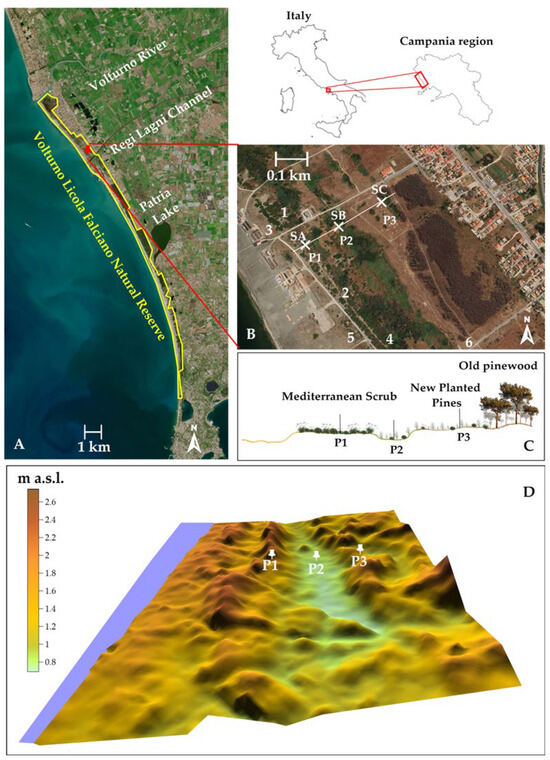
Figure 1.
(A) Sentinel-2 true color mosaic image of the study area showing the boundaries (yellow line) of the “Volturno Licola Falciano Natural Reserve” and the location (red point) of the experimental field; (B) Google Earth image of the experimental field showing piezometer locations (P1, P2, and P3), soil profile locations (SA, SB, SC), and soil sample locations (1, 2, 3, 4, 5, and 6); (C) cross-sectional diagram indicating the experimental area zonation and the piezometer locations (P1, P2, and P3); (D) DTM of the experimental field.

Table 1.
Soil chemical and physical characteristics of the studied area.
The plant community is characterized by an afforested 80-year-old pine forest, composed mainly of stone pine forest (Pinus pinea L.) together with maritime pine (Pinus pinaster Aiton.), in association with a few specimens of Aleppo pine (Pinus halepensis Mill.), holm oak (Quercus ilex L.), and Mediterranean scrub plants [36]. The pine forest has suffered a dramatic loss of trees in recent years [37]. In 2023, new pine trees were planted, with a larger planting layout, and interspersed with Mediterranean bushes to replace the dead pines according to the HD guidelines. Aware that persistent anticyclonic conditions generated exceptional dryness in 2022 [6], the newly planted plants were irrigated daily (3 L per plant) with local groundwater (0.8 g/L of TDS), and their growth was monitored weekly starting from 2023.
2.2. Sentinel-2 and Meteorological Data Collection
Global Mosaic Service (GMS) Sentinel-2 is an ESA mission aimed at systematically providing high-resolution multispectral imagery of global terrestrial surface. Imagery and data were freely downloaded from the Copernicus Browser [38]. Sentinel-2 L2A NDVI and NDMI data with a pixel size of 10 m and 20 m, respectively, were collected every 5 days, while annual images (each October) were extracted from 2016 to 2023. Only the images and the data with a cloud coverage < 10% were retained. NDVI quantifies green vegetation and photosynthetic capacity and ranges between −1 and 1. Negative values approaching −1 indicate water bodies, values close to 0 indicate barren areas, values between 0.2 and 0.4 indicate grassland, those between 0.4 and 0.6 indicate shrubland, and those >0.6 indicate temperate and tropical forests [39]. NDVI is calculated as follows:
For Sentinel-2, NIR corresponds to band B8A, and RED corresponds to band B04.
NDMI is a moisture index deployed as a proxy of leaf water content that uses NIR and SWIR bands to display moisture [40]. This combination is able to remove the variations caused by leaves internal structure and leaves dry matter content, ameliorating the accuracy of vegetation’s water content detection. It ranges between −1 and 1. Negative values of NDMI (approaching −1) correspond to bare soil, values between −0.2 and 0 correspond to critical water stress, values between 0 and 0.2 correspond to high water stress, those between 0.2 and 0.4 correspond to low water stress, and those >0.6 correspond to no water stress. NDMI is calculated as follows:
For Sentinel-2, NIR corresponds to band B08, and SWIR corresponds to band B11.
Daily mean, minimum, maximum temperature, and precipitation data from 2014 to 2023 were extracted from the records of the “Centro Funzionale Multirischi della Protezione Civile Regione Campania” [41]. Actual evapotranspiration (AET) and potential evapotranspiration (PET) data were downloaded from EARTHDATA website (https://www.earthdata.nasa.gov/) by selecting the Moderate Resolution Imaging Spectroradiometer (MODIS) instrument of the National Aeronautics and Space Administration (NASA) with a pixel size of 500 m [42].
The integration of Sentinel-2 data, meteorological data, and field data was achieved by comparing trends over time. RS data trends were compared with meteorological data for the same periods and with field data for the monitoring time window.
2.3. Soil Sampling and Analysis
Soil samples were collected at five different depths (0–20 cm; 20–40 cm; 40–60 cm; 60–80 cm; 80–100 cm) in October and December 2023 to obtain three complete soil salinity profiles (SA, SB, SC; Figure 1B). Three replicas were obtained for each depth to obtain statistical significance. A total number of 45 samples were collected in each date of sampling for porewater Total Dissolved Solids (TDSpw) analyses. Batch extractions were performed on the 45 samples collected, following the saturation soil extraction (SSE) method [43]. Each batch had a liquid/solid (L/S) ratio of 5:1 to ensure total ion dissolution [44], with the liquid phase, consisting of Milli-Q deionized water (18 MΩ). The high-density polyethylene containers for the batches were sealed to prevent external influences and kept in darkness at a regulated temperature of 25 ± 1 °C until the equilibrium was reached. TDS was then detected using a HANNA multi-parameter probe (model HI98194). TDSpw were calculated using the following formula [45]:
where d is the dilution factor due to the batch L/S ratio, TDS are the total dissolved solids in the liquid phase of the batches (g/L), ρb is the dry bulk density of the sample measured (g/cm3), and n is the total porosity of the measured sample (-).
2.4. Groundwater and Vadose Zone Monitoring
The experimental field was instrumented with 3 piezometers (P1, P2, and P3) lined up perpendicular to the shoreline (Figure 1). Distance between P1 and P2 was 165 m, while distance between P2 and P3 was 101 m. Each piezometer consisted of a 2 m long polyethylene tube with internal diameter of 3 cm and slotted with a screen of 10 cm at its bottom, covered with a nitex 50 µm mesh to prevent clogging. Piezometers were installed to a depth of 1.5 m with a motor auger and then equipped with a water level data logger to monitor groundwater level (H), temperature (T), and TDS (Soil & Water Diver® from Eijkelkamp, Giesbeek, The Netherlands). Data were corrected for atmospheric pressure changes via a Barologger® (Eijkelkamp, Giesbeek, The Netherlands) placed at the soil surface close to P3. For each parameter of each diver, 12,710 data were collected through continuous direct measurements, reaching a total of 114,390 data. Data recording was set at 30 min intervals, and the monitoring period ran from March 2023 to November 2023. In the vicinity of P3, four probes were installed in the soil at 10, 20, 30, and 40 cm depth to monitor volumetric water content (VWC), temperature, and Soil Bulk Electrical Conductivity (ECb) of the vadose zone. The probes were 5TE® type from Meter (Meter Environment, Pullman, WA, USA) and used a data logger to store the data. Data recording was set at 30 min intervals, and the monitoring period ran from March 2023 to September 2023. For each parameter and for each depth, the data logger stored 7364 data for a total of 95,732 data collected through continuous direct measurements. Then, ECb was corrected in EC according to the model of Hilhorst (2000) [46] using the following formula:
where is the complex porewater permittivity at a given temperature, is the real part of the bulk soil permittivity, and the offset can be calculated from the and ECb values measured at two arbitrary free water content values. Subsequently, EC was converted into TDS using the standard linear conversion factor of 0.66 [47].
2.5. Wet Deposition Sampling and Flux Calculation
Bulk dry and wet deposimeter samplers (Nesa srl, Vidor, Treviso, Italy) were installed close to each piezometer for periodic monitoring of precipitation chemistry. Samples were collected from the deposimeter every three months. Then, samples were analyzed for anions and cations with an ICS-1000 Dionex (Thermo-Fisher, Waltham, MA, USA). An AS-40 Dionex auto-sampler was used to load the samples. Quality Control (QC) samples were integrated into the analysis routine, with QC samples analyzed every 3 samples to ensure the accuracy and reliability of the results. The bulk concentration was converted in wet-only concentration using the correction factors proposed by Staelens et al. (2005) for field samplings [48]. Finally, the daily average deposition flux (Fω) in mg/m2 of the main marine aerosol components (Na+, Cl−, and SO42−) [12] was calculated using the following formula [49]:
where C is the element concentration corrected for the wet deposition in mg/L, and P is the amount of precipitation in the interested area in L/m2.
2.6. Data Analysis
Locally Estimated Scatterplot Smoothing (LOESS) regression was calculated on NDVI and NDMI data using Statgraphics Centurion 19 to better explore the non-linear trend. LOESS is defined by Span, Family, and Degree. Span represents the proportion of data used to fit the local polynomial at each point. Family specifies the fitting algorithm. Degree specifies the order in which the local polynomials are fitted to each data subset. The Span was set to 0.5. Gaussian was chosen as the Family using least squares fit. The Degree was set to 2 to fit a quadratic function to each data subset.
A simple NDVI qualitative accuracy assessment was carried out through periodical field observations of old and new pines. NDMI quantitative accuracy assessment was carried out using soil volumetric water content (VWC) data from April 2023 to August 2023. Root Mean Square Error (RMSE), Mean Absolute Error (MAE), and accuracy percentage were calculated through linear_model and sklearn.metrics python modules of the scikit-sklearn package importing pandas and numpy libraries.
3. Results
3.1. Sentinel-2 Monitoring
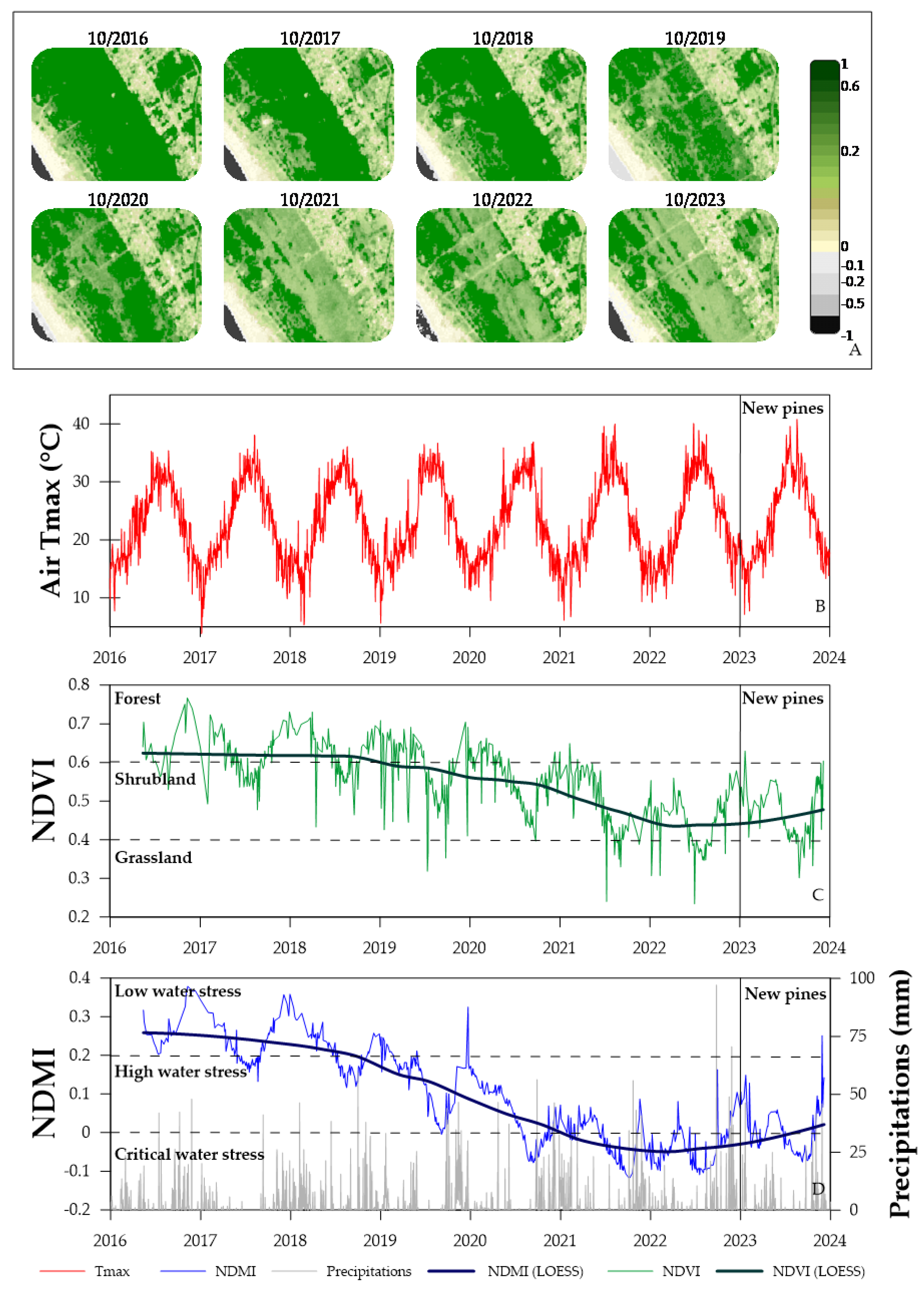
Sentinel 2-LA2 imagery reveals that the highest canopy and vegetation health decrease occurred between 2020 and 2021 (Figure 2A). The NDVI trend clearly indicates the pine forest decline shifting from values typical of forest (>0.6) in 2016 to values characteristic of shrubland (0.4–0.6) at the end of 2020, reaching lower peaks between 2021 and 2023, even assuming grassland values (<0.2) (Figure 2C). The NDVI and maximum temperatures (Tmax) show opposite trends (Figure 2B,C), with NDVI peaks during periods with lower Tmax.

Figure 2.
(A) Annual Sentinel-2 L2A NDVI images of each October of the old pine forest in the experimental field from 2016 to 2024; (B) Air Tmax trend (red line) from 2016 to 2024. The black vertical line indicates the new pines’ plantation date; (C) NDVI trend (light green line) and NDVI LOESS line (dark green line) from 2016 to 2024. The horizontal dashed black lines indicate the forest/shrubland interface and the shrubland/grassland interface on the basis of NDVI values, while the vertical black line indicates the new pines’ plantation date; (D) NDMI trend (blue line), NDVI LOESS line (dark blue line), and daily precipitation pattern (gray line) from 2016 to 2024. The horizontal dashed black lines indicate the level of water stress intervals, while the vertical black line indicates the new pines’ plantation date.
During the monitoring period, there was a slight increase (1.5%) in Tmax (Figure 2B), with a remarkable increase in days with Tmax > 35 °C in 2021 (Figure S1 in the Supplementary Materials), and 19 days of Tmax > 35 °C in 2021 against the 7 days recorded in 2020.
The NDMI trend (Figure 2D) reveals how, beginning in mid-2019, the pine forest entered a permanent state of high water stress (0.0 < NDMI < 0.2), with alternating periods of critical water stress (NDMI < 0.0) from late 2020 to late 2023. Moreover, the lowest peaks of NDMI were observed in the 2021 and 2022 summers after prolonged drought periods.
Further confirmation of this persistent water stress status is given by MODIS AET data (Figure S2 in the Supplementary Materials), whose trend mimicked NDMI, showing a significant decrease in 2020 and reaching the lowest values in 2021, while the PET trend was substantially constant since PET is not affected by the plant status.
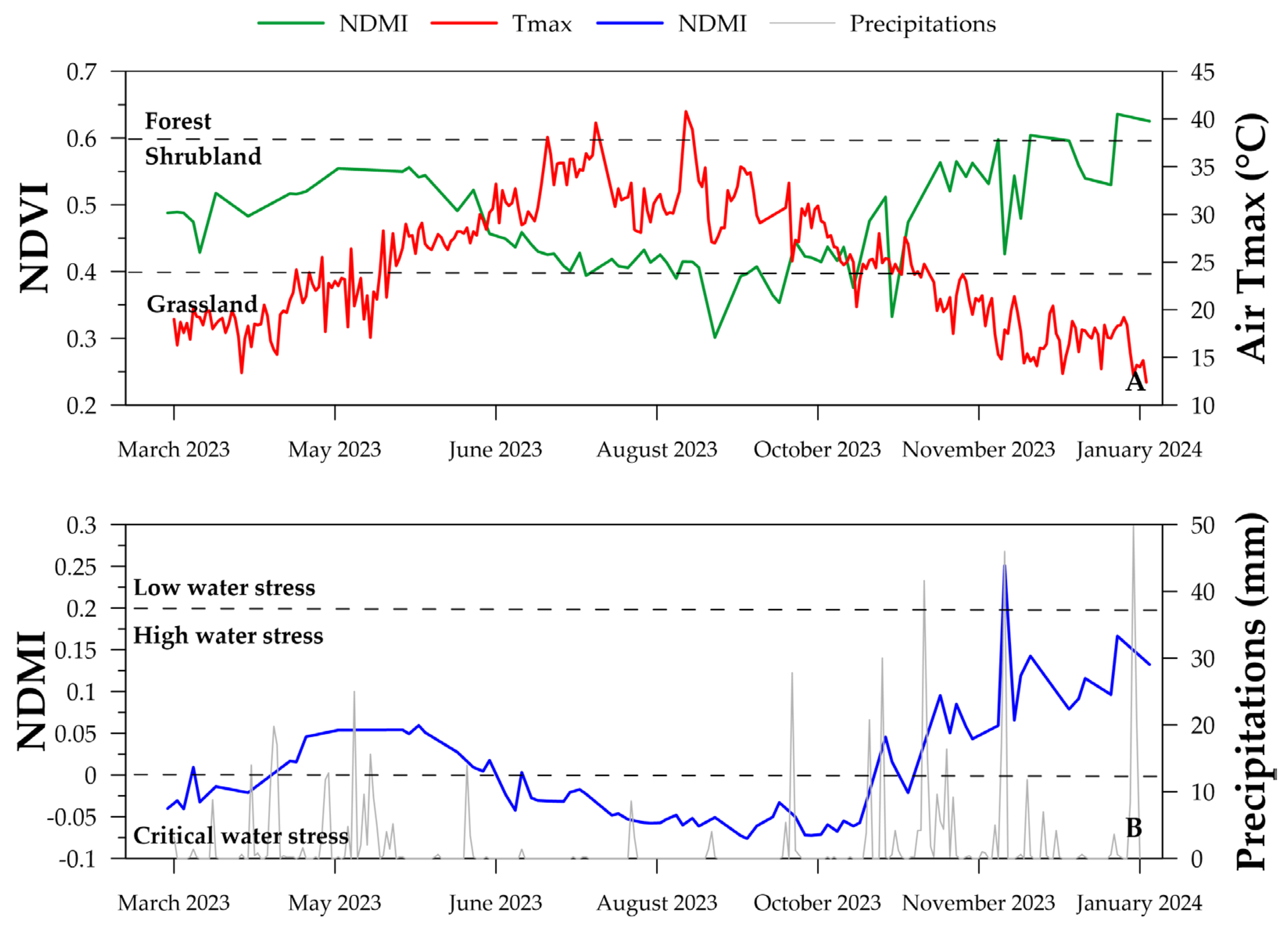
Figure 3 depicts NDVI and NDMI trends zoomed from March 2023 to January 2024, which correspond to the monitoring period of the new plantation growth. It is evident that the NDVI shows an inverse trend to that of Tmax. Indeed, the NDVI trend reveals a first canopy increase until the beginning of June 2023, when the increase in the temperature combined with scarce precipitation generated a rapid decrease in the NDVI, even dropping below the shrubland/grassland interface. The decrease in temperature and the increase in precipitation enhanced water availability, and the NDVI increased, reaching the shrubland/forest interface at the end of 2023, indicating canopy growth of the vegetation. The NDMI trend mimicked the NDVI (Figure 3B), increasing at the beginning of 2023, reaching critical water stress values for the summer period, and rising by the end of October 2023, when the abundant precipitation generated a reduction in water stress. In fact, the AET trend (Figure S2 in the Supplementary Materials) increased at the end of 2023, suggesting an upswing in plant activity.

Figure 3.
(A) NDVI trend (green line) from March 2023 to January 2024 and daily Tmax trend (red line). The dashed black lines indicate the forest/shrubland interface and the shrubland/grassland interface on the basis of NDVI values; (B) NDMI trend (blue line) from March 2023 to January 2024 and daily precipitation pattern (gray line). The dashed black lines indicate the level of water stress intervals.
3.2. Field Monitoring
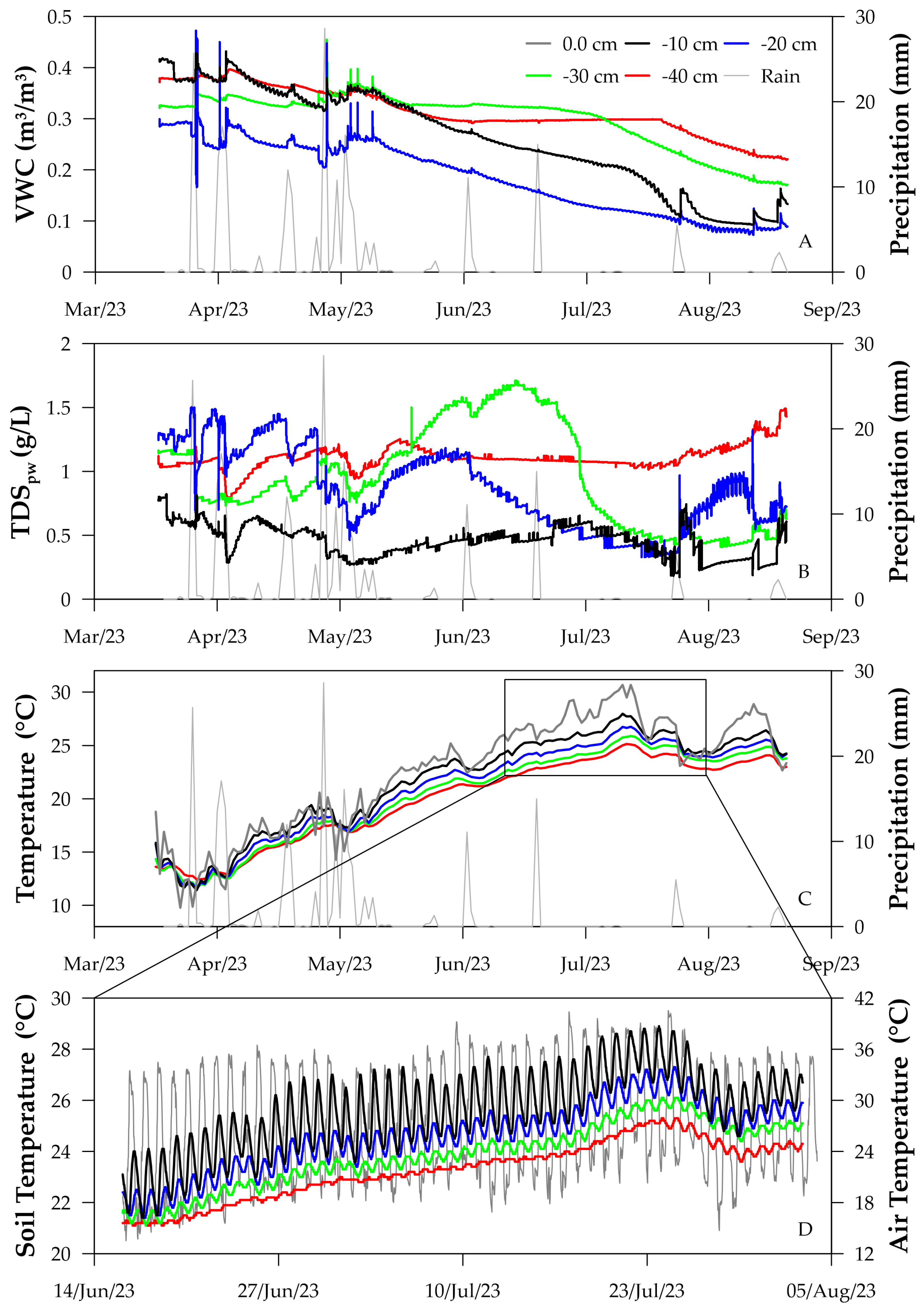
The vadose zone monitoring reveals a depth-progressive drop in the VWC (Figure 4A). The decrease in the VWC started at −10 and −20 cm because of the double effect of scarce precipitation and plant root water suction. Upon reaching critical VWC values (<0.2 m3/m3) at −10 and −20 cm, a progressive VWC decrease was observed at −30 cm and subsequently at −40 cm. This happened because there was insufficient water available for plants in the first 20 cm; hence, roots began to extract water from deeper soil horizons. This is despite daily irrigation, which was recorded by the sensors at −10 and −20 cm with small fluctuations. Plants’ water suction combined with the high temperatures recorded during the monitoring period (Figure 4C), even reaching atmospheric temperature peaks of 40 °C (on the soil surface) and a vadose zone temperature of 28 °C (at −10 cm) at the end of July (Figure 4D), triggered salt evapoconcentration in the vadose zone. Indeed, the depth-progressive plants’ water suction is further confirmed by the salt movement through the vadose zone. Initially, the highest TDS values were observed at −20 cm, while, when the roots started to draw water from the deeper layer, TDS peaks were observed at −30 cm and finally at −40 cm at the end of the monitoring period. TDS at −10 cm has been kept lower and more stable by daily irrigation with 0.8 g/L of water. The infiltration of irrigation water also contributed to the salt leaching into the underlying strata, with the largest salinity peaks observed between −30 cm and −40 cm.
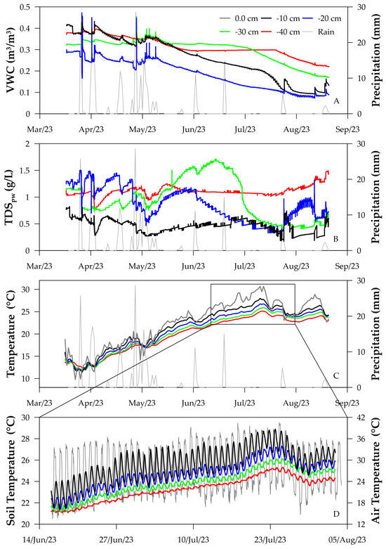
Figure 4.
(A) Volumetric water content (VWC) of the vadose zone from March to September 2023 at different depths (−10; −20; −30; −40 cm) and daily precipitation (gray line); (B) TDS of the vadose zone from March to September 2023 at different depths (−10; −20; −30; −40 cm) and daily precipitation (gray line); (C) average daily temperature of the vadose zone at different depths (0.0; −10; −20; −30; −40 cm) from March to September 2023 and daily precipitation (gray line); (D) daily oscillations of the vadose zone temperature at different depths (−10; −20; −30; −40 cm) and the air temperatures (gray line) from June to August 2023.
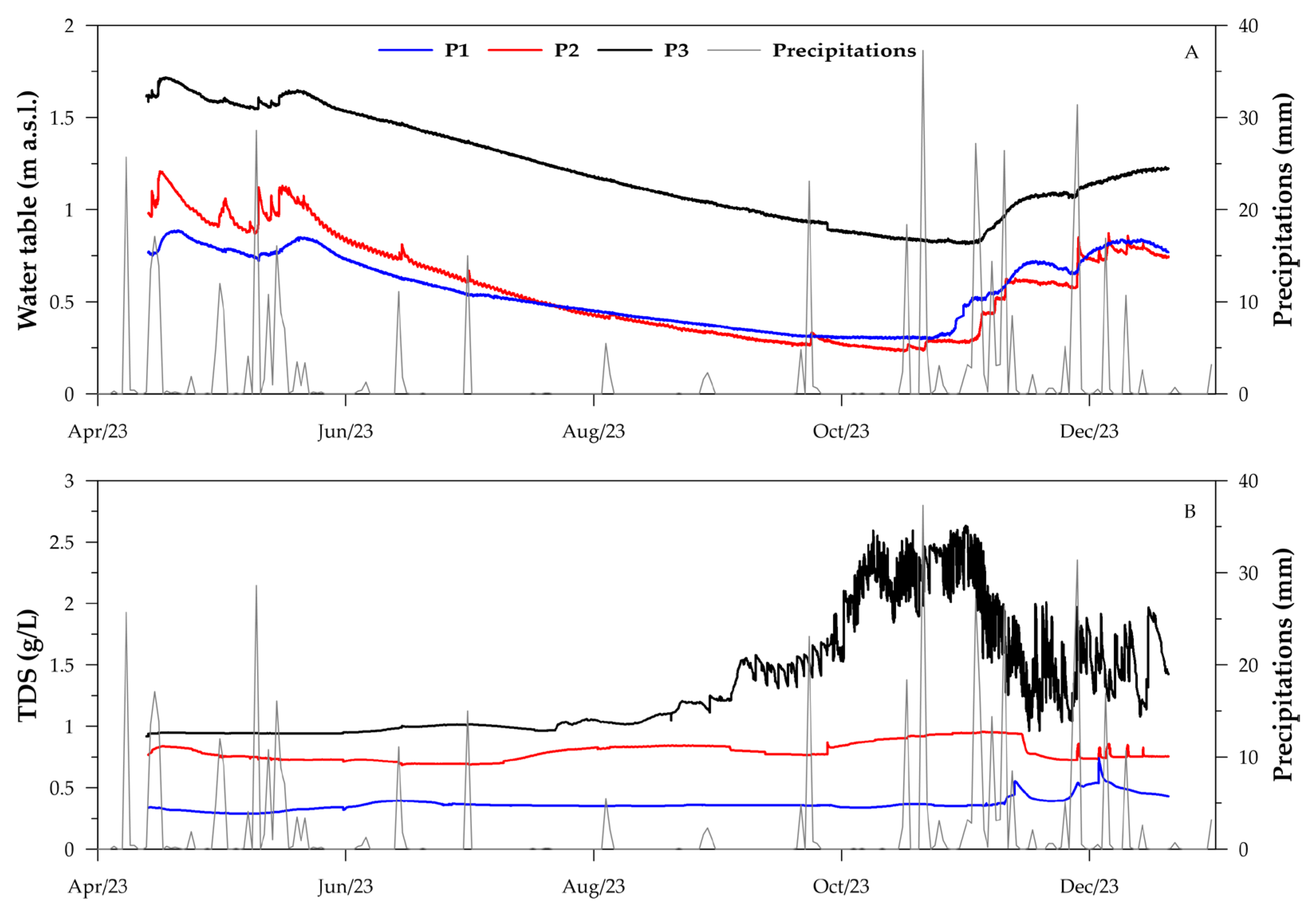
The results of the shallow groundwater monitoring showed that the groundwater salinity was low (0.35–0.40 g/L) near the shoreline since the dunes allowed for rapid rainwater infiltration and deep drainage, preventing seawater intrusion (Figure 5), also indicating the effectiveness of the dunes in blocking the marine spray deposition. P3 showed the highest values of TDS (2.5–2.75 g/L) between the end of October and the beginning of November 2023. Groundwater levels (H) clearly reveal that groundwater is moving from inland (P3) to the shoreline (P1) since H always followed the scale of H(P3) > H(P2) > H(P1) during the whole monitoring period. Only the persistent precipitation in November 2023 that completely saturated the dunes generated intervals with H values higher in P1 than in P2 (but never surpassing H in P3). The direction of groundwater flow combined with a lower groundwater TDS close to the shoreline further indicates that the salinity detected in the pine forest is not attributable to saltwater intrusion into the shallow aquifer but to salt evapoconcentration created by plant water withdrawal combined with a persistent period of high temperature. Because the soil texture is prevalently coarse sand, the excessive rainfall during the last period of monitoring resulted in significant water infiltration and deep drainage, dragging the salt trapped into the vadose zone downward to the saturated zone.
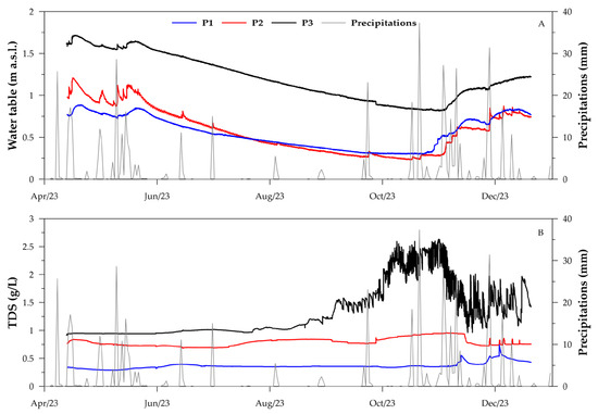
Figure 5.
(A) Water table level from March to December 2023 in the 3 piezometers P1, P2, and P3, and daily precipitation (gray line); (B) groundwater TDS from March to December 2023 in the 3 piezometers P1, P2, and P3, and daily precipitation (gray line).
The groundwater monitoring results are consistent with the soil salinity profiles (Figure S3 in the Supplementary Materials) in October 2023 and December 2023. In both sampling campaigns, higher TDSpw were detected in SC, which is the more inland profile, confirming evapoconcentration as the main driver of salt accumulation in the soil and ruling out that salinity origin may derive from marine intrusion. The sampling campaign of December 2023 shows lower TDS values within all the profiles in comparison to the values of October 2023, confirming the downward movement of salt transported by the infiltrating water.
3.3. Marine Spray Wet Deposition Flux
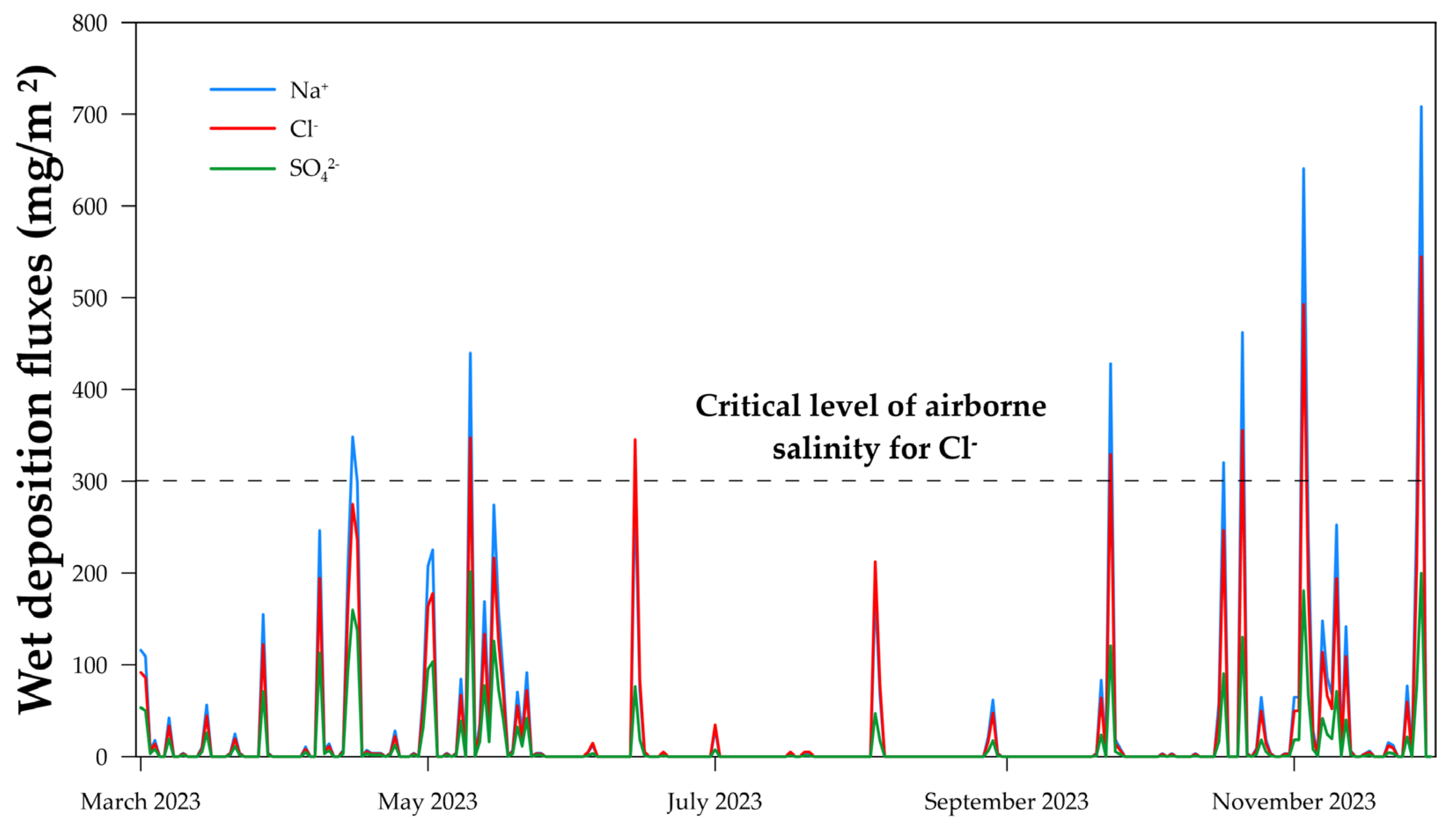
In Figure 6, the wet deposition flux of marine spray is shown. The largest values were detected in the period between the end of October 2023 and the beginning of November 2023, when persistent storm conditions allowed massive salt spray deposition. During this period, Cl− and Na+ repeatedly showed values greater than 400 mg/m2. Indeed, in four storm events that occurred between October and November 2023, the critical level of airborne salinity represented by Cl− wet deposition flux (300 mg/m2) [50] was largely overstepped.
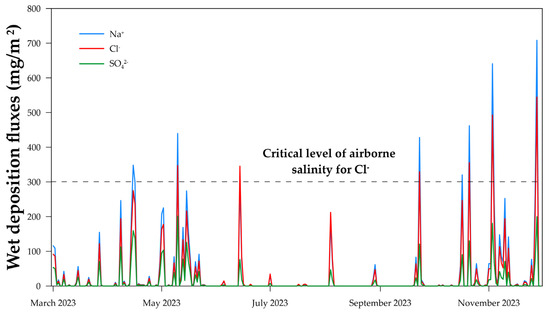
Figure 6.
Na+ (blue line), Cl− (red line), and SO42− (green line) wet deposition fluxes from March to December 2023. The dashed black line represents the critical level of airborne salinity for Cl− following the international standard ISO 9223:2012.
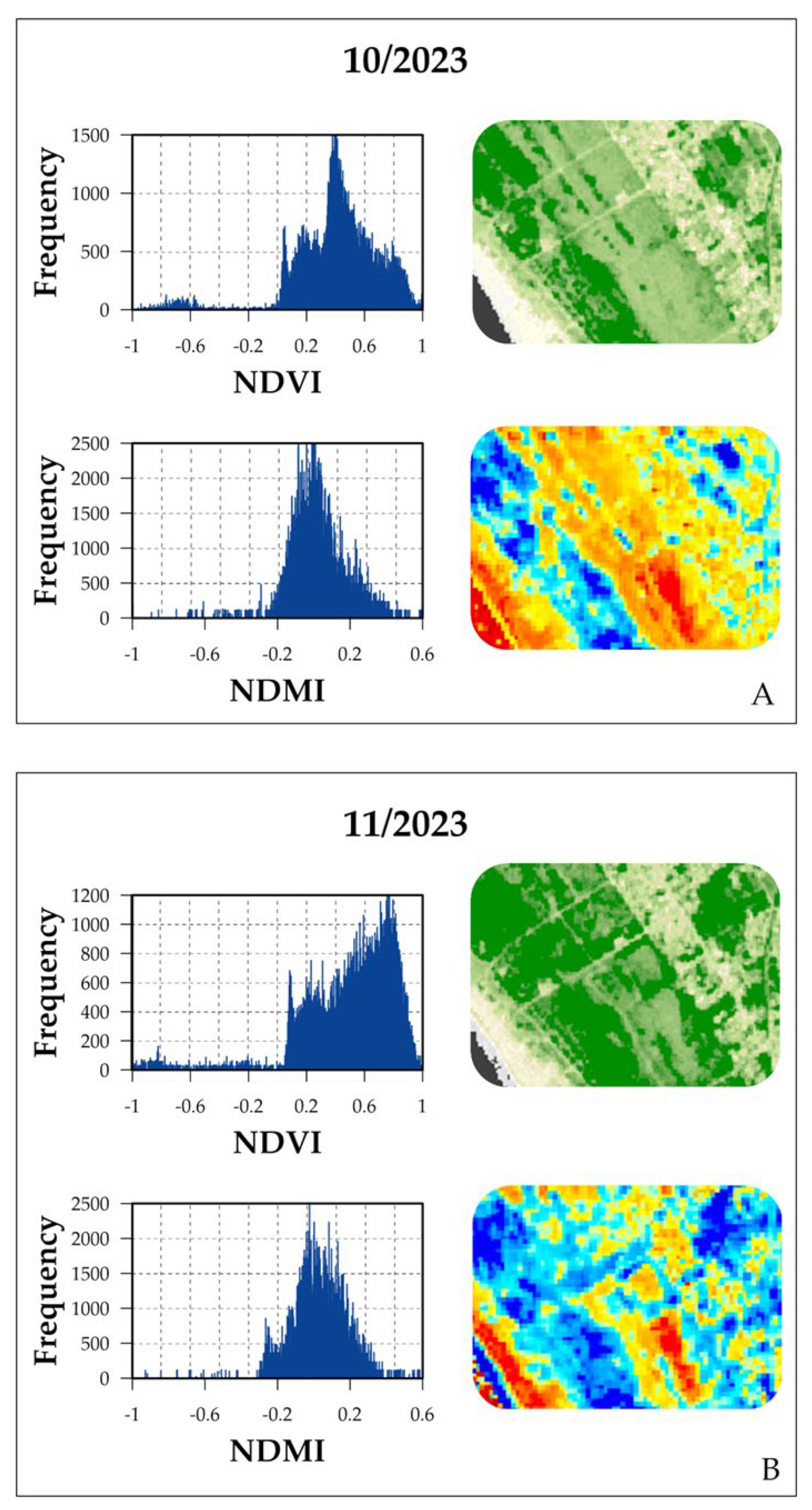
NDVI and NDMI images pre and post mid-November 2023 storms, combined with the shift in pixel frequency histograms toward higher values, show an increase in the photosynthetic activity of the vegetation canopy and a decrease in water stress (Figure 7). Despite this period, field observations revealed a dramatic photosynthetic activity loss (about 40%) for the new pines during November. This underlines one of the main limitations of RS monitoring, being not able to discriminate different species, since they may exhibit identical spectral responses [26]. The persistent and intensive storm events allowed salt spray deposition that completely desiccated the seaward exposed part of newly planted pines (Figure S4 in the Supplementary Materials) [13]. Indeed, the growth of young pine trees can be affected by high doses of Cl− deposition and even dying prematurely [51], particularly in the aftermath of extreme storm events [13]. Although most plants have recovered from the damage of the November storms, during the field monitoring at the end of December, 15% mortality of the newly planted pines was detected.

Figure 7.
(A) NDMI and NDVI images and pixel frequency histograms of NDMI and NDVI pre-storm (10/2023); (B) NDMI and NDVI images and pixel frequency histograms of NDMI and NDVI post-storm (11/2023).
4. Discussion
RS monitoring with Sentinel 2 imagery and data has effectively detected the gradual decline in the old pine forest (Tables S1 and S2 in the Supplementary Materials). On the one side, NDMI clearly showed how the pines were in a constant state of water stress; on the other side, NDVI was effective in capturing the pine forest canopy decrease. Due to the high water stress status, the pine forest’s canopy activity started to decrease gradually in 2017. Accordingly, long and severe drought is the most extended driver of pine mortality in the Mediterranean Basin [52]. The dramatic rise in temperature in 2021, combined with the protracted drought, proved to be a fatal stressor to the aged pine forest, whereas temperatures higher than 35 °C could cause stomatal closure, limiting gas exchange and irreversibly damaging the photosynthetic apparatus [53]. Moreover, the pine forest was already facing several stresses: (i) the high-density plantation layout (2 m × 3 m, 2 m × 4 m, 3 m × 3 m totaling 2500 trees/ha) that could have exacerbated the water stress, since density larger than 500–1000 trees/ha can have negative impact on plant moisture content [54]; and (ii) the proven presence of Tomeyella parvicorsis (Cockerel), known as the pine tortoise scale insect, in this area since 2015, that made the already fragile pine forest even more susceptible to further stress [55]. In the same area, Niccoli et al. (2024) [56], using an integrating approach between dendrochronological, isotopic, and remote sensing analysis, revealed the physiological responses of Pinus pinea L. to Tomeyella parvicorsis (Cockerel), identifying the first signs of tree decline and the critical moments that led to the death of the plantation, mainly due to the pest outbreak. Pest attacks and outbreaks are usually the consequence of a progressive weakening of vegetation due to other kinds of stresses. In fact, the most vulnerable plants are those attacked by pests, at least at first. Rubio-Cuadrado et al. (2021) [57] reported several Greek pine forest deaths between 2016 and 2019 because of combined influences of pests, drought, and excessive plantation density.
In the study area, salinity stress, although not the main driver, was an additional pressure. Salt, delivered through wet and dry deposition of sea spray [58] and through irrigation water [59], was subsequently evapoconcentrated by plant roots [60]. As a result, when rainfall becomes abundant, the rapid water infiltration and deep drainage over the sandy soil profile leads to salt leaching and thus an increase in groundwater salinity [61]. The threshold limit of water TDS values for plant growth (2.5 g/L) [62] was slightly overcome only in a small window of the monitoring period, confirming that groundwater and soil salinity cannot be the main drivers of the old pine forest demise, but could have represented an additional stress. Inversely, these constraints could be an issue for the newly planted pine forest, considering that young plants are more salt-susceptible than adult ones [63].
Salt spray fluxes generally decrease from the end of the spring to late summer before rapidly increasing during autumnal storms [64]. However, alternating periods of severe storms and low precipitation could accentuate the negative impact of Cl− deposition since salt wash-out could be limited [65]. Similar results were found by Raddi et al. (2009) [66], which investigated the depletion of an Italian coastal Pinus pinea L. forest (in Tuscany), identifying sea spray exposure as the primary cause of foliage mortality. Instead, the Mediterranean pioneer vegetation was not affected by these combined salinity stress conditions because of its halophytic resistance [67], and its canopy development rendered the detection of young pines’ stress through RS monitoring ineffective. These results depict an important warning for the management of Mediterranean pine forests, given that the Intergovernmental Panel on Climate Change (IPCC) projections for the Mediterranean region [68] predicted an increase in the frequency and intensity of abnormal storm surges in the next years, representing a non-negligible issue for the preservation of pines and other salt-susceptible species.
5. Conclusions
This study documented the decline in the pine forest of the “Volturno Licola Falciano Natural Reserve” through remote sensing (RS) and field monitoring, quantifying the main stressors that contributed to this phenomenon. Increased temperature and prolonged periods of water stress were the driving factors of the old pine forest extinction, while salinity stress was just an additional stressor. RS was useful to precisely locate the area of pine forest gradual stress and death using NDVI and NDMI, but RS data alone were not able to identify the vegetation stress of newly planted pines, as depicted in the accuracy assessment, since the main indices were affected by the Mediterranean shrubs’ growth. Thus, RS data must be validated with field-based data to correct biases and avoid misinterpretations. Indeed, while Sentinel-2’s spatial resolution was suitable for most study purposes, including the old pine forest monitoring, it had major constraints for new pine forest monitoring. For instance, the resolution was insufficient to discern differences in responses to environmental stress across the many plant species found in the new pine plantation. Sentinel-2 was unable to accurately capture physiological differences due to the greater heterogeneity of the species and the small size of the individual vegetation patches, compromising the achievement of some specific objectives related to the monitoring of the new pines. Therefore, it is preferable to use RS to monitor resilient adult forests for which there is time to plan interventions and contrast the perish. Conversely, in stress-susceptible phases, such as early growth, RS should be coupled with field-based monitoring to promptly identify any criticalities. The proposed coupled monitoring could be largely adopted to understand the main causes of plants’ salinity stress in many other coastal environments.
Supplementary Materials
The following supporting information can be downloaded at: https://www.mdpi.com/article/10.3390/rs16173150/s1, Figure S1: (A) Number of days with Tmax > 30 °C from 2019 to 2023; (B) Number of days with Tmax > 35 °C from 2019 to 2023; Figure S2: AET trend (blue line) and PET trend (black line) from 2015 to 2024; Figure S3: TDSpw values at different depths of three soil profiles (SA, SB, and SC) for two sampling campaigns, one in October 2023 (left panel) and one in December 2023 (right panel); Figure S4: Desiccated young pines detected during field inspection in November 2023; Table S1: Qualitative accuracy assessment of NDVI data; Table S2: Quantitative accuracy assessment of NDMI data using VWC data as proxy.
Author Contributions
Conceptualization, N.C., S.F. and M.M.; methodology, L.A. and N.C.; software, L.A. and N.C.; validation, M.M., E.G. and S.F.; formal analysis, L.A.; investigation, L.A. and N.C.; resources, M.M., N.C. and S.F.; data curation, L.A. and N.C.; writing—original draft preparation, L.A. and E.G.; writing—review and editing, N.C. and M.M.; visualization, L.A. and N.C.; supervision, M.M.; project administration, S.F. All authors have read and agreed to the published version of the manuscript.
Funding
This research received no external funding.
Data Availability Statement
The raw data supporting the conclusions of this article will be made available by the authors on request.
Acknowledgments
The authors would like to express their gratitude to the President and officials of the Volturno, Licola, and Falciano Natural Reserve for their cooperation and support during this research. Additionally, the authors would like to thank the A.T.S. Monte Maggiore cooperative of Orsara (Puglia region, Italy) for their technical and operational assistance.
Conflicts of Interest
The authors declare no conflicts of interest.
References
- Van Der Maarel, E. Some Remarks on the Functions of European Coastal Ecosystems. Phytocoenologia 2003, 33, 187–202. [Google Scholar] [CrossRef]
- Sperandii, M.G.; Bazzichetto, M.; Gatti, F.; Acosta, A.T.R. Back into the Past: Resurveying Random Plots to Track Community Changes in Italian Coastal Dunes. Ecol. Indic. 2019, 96, 572–578. [Google Scholar] [CrossRef]
- Carranza, M.L.; Acosta, A.T.R.; Stanisci, A.; Pirone, G.; Ciaschetti, G. Ecosystem Classification for EU Habitat Distribution Assessment in Sandy Coastal Environments: An Application in Central Italy. Environ. Monit. Assess. 2008, 140, 99–107. [Google Scholar] [CrossRef] [PubMed]
- Jolicoeur, S.; O’Carroll, S. Sandy Barriers, Climate Change and Long-Term Planning of Strategic Coastal Infrastructures, Îles-de-La-Madeleine, Gulf of St. Lawrence (Québec, Canada). Landsc. Urban Plan. 2007, 81, 287–298. [Google Scholar] [CrossRef]
- Sun, C.; Liu, Y.; Zhao, S.; Li, H.; Sun, J. Saltmarshes Response to Human Activities on a Prograding Coast Revealed by a Dual-Scale Time-Series Strategy. Estuar. Coast. 2017, 40, 522–539. [Google Scholar] [CrossRef]
- Faranda, D.; Pascale, S.; Bulut, B. Persistent Anticyclonic Conditions and Climate Change Exacerbated the Exceptional 2022 European-Mediterranean Drought. Environ. Res. Lett. 2023, 18, 034030. [Google Scholar] [CrossRef]
- Jones, M.L.M.; Sowerby, A.; Williams, D.L.; Jones, R.E. Factors Controlling Soil Development in Sand Dunes: Evidence from a Coastal Dune Soil Chronosequence. Plant Soil 2008, 307, 219–234. [Google Scholar] [CrossRef]
- Bazzichetto, M.; Malavasi, M.; Acosta, A.T.R.; Carranza, M.L. How Does Dune Morphology Shape Coastal EC Habitats Occurrence? A Remote Sensing Approach Using Airborne LiDAR on the Mediterranean Coast. Ecol. Indic. 2016, 71, 618–626. [Google Scholar] [CrossRef]
- Fitzgerald, J.W. Marine Aerosols: A Review. Atmos. Environ. 1991, 25, 533–545. [Google Scholar] [CrossRef]
- Cerrato, M.; Ribas-Serra, A.; Cortés-Fernández, I.; Cardona Ametller, C.; Mir-Rosselló, P.M.; Douthe, C.; Flexas, J.; Gil, L.; Sureda, A. Effect of Seawater Salinity Stress on Sporobolus Pungens (Schreb.) Kunth, a Halophytic Grass of the Mediterranean Embryonic Dunes. Plant Growth Regul. 2022, 98, 191–204. [Google Scholar] [CrossRef]
- Mastrocicco, M.; Colombani, N. The Issue of Groundwater Salinization in Coastal Areas of the Mediterranean Region: A Review. Water 2021, 13, 90. [Google Scholar] [CrossRef]
- Alessandrino, L.; Gaiolini, M.; Cellone, F.A.; Colombani, N.; Mastrocicco, M.; Cosma, M.; Da Lio, C.; Donnici, S.; Tosi, L. Salinity Origin in the Coastal Aquifer of the Southern Venice Lowland. Sci. Total Environ. 2023, 905, 167058. [Google Scholar] [CrossRef]
- Du, J.; Hesp, P.A. Salt Spray Distribution and Its Impact on Vegetation Zonation on Coastal Dunes: A Review. Estuar. Coasts 2020, 43, 1885–1907. [Google Scholar] [CrossRef]
- Peñuelas, J.; Sardans, J.; Filella, I.; Estiarte, M.; Llusià, J.; Ogaya, R.; Carnicer, J.; Bartrons, M.; Rivas-Ubach, A.; Grau, O.; et al. Impacts of Global Change on Mediterranean Forests and Their Services. Forests 2017, 8, 463. [Google Scholar] [CrossRef]
- Conte, A.; Zappitelli, I.; Fusaro, L.; Alivernini, A.; Moretti, V.; Sorgi, T.; Recanatesi, F.; Fares, S. Significant Loss of Ecosystem Services by Environmental Changes in the Mediterranean Coastal Area. Forests 2022, 13, 689. [Google Scholar] [CrossRef]
- EEC Council Directive 92/43/EEC; The Conservation of Natural Habitats and of Wild Fauna and Flora. 1992.
- Torres, I.; Moreno, J.M.; Morales-Molino, C.; Arianoutsou, M. Ecosystem Services Provided by Pine Forests. In Pines and Their Mixed Forest Ecosystems in the Mediterranean Basin. Managing Forest Ecosystems; Ne’eman, G., Osem, Y., Eds.; Springer: Cham, Switzerland, 2021; Volume 38, pp. 617–629. [Google Scholar]
- Quinto, L.; Navarro-Cerrillo, R.M.; Palacios-Rodriguez, G.; Ruiz-Gómez, F.; Duque-Lazo, J. The Current Situation and Future Perspectives of Quercus Ilex and Pinus Halepensis Afforestation on Agricultural Land in Spain under Climate Change Scenarios. New For. 2021, 52, 145–166. [Google Scholar] [CrossRef]
- Lechner, A.M.; Foody, G.M.; Boyd, D.S. Applications in Remote Sensing to Forest Ecology and Management. One Earth 2020, 2, 405–412. [Google Scholar] [CrossRef]
- Lawley, V.; Lewis, M.; Clarke, K.; Ostendorf, B. Site-Based and Remote Sensing Methods for Monitoring Indi-cators of Vegetation Condition: An Australian Review. Ecol. Indic. 2016, 60, 1273–1283. [Google Scholar] [CrossRef]
- Xie, Y.; Sha, Z.; Yu, M. Remote Sensing Imagery in Vegetation Mapping: A Review. J. Plant Ecol. 2008, 1, 9–23. [Google Scholar] [CrossRef]
- Marzialetti, F.; Giulio, S.; Malavasi, M.; Sperandii, M.G.; Acosta, A.T.R.; Carranza, M.L. Capturing Coastal Dune Natural Vegetation Types Using a Phenology-Based Mapping Approach: The Potential of Sentinel-2. Remote Sens. 2019, 11, 1506. [Google Scholar] [CrossRef]
- Strashok, O.; Ziemiańska, M.; Strashok, V. Evaluation and Correlation of Normalized Vegetation Index and Moisture Index in Kyiv (2017–2021). J. Ecol. Eng. 2022, 23, 212–218. [Google Scholar] [CrossRef]
- Dutkiewicz, A.; Lewis, M.; Ostendorf, B. Evaluation and Comparison of Hyperspectral Imagery for Mapping Surface Symptoms of Dryland Salinity. Int. J. Remote Sens. 2009, 30, 693–719. [Google Scholar] [CrossRef]
- Ramsey, E.; Werle, D.; Suzuoki, Y.; Rangoonwala, A.; Lu, Z. Limitations and Potential of Satellite Imagery to Monitor Environmental Response to Coastal Flooding. J. Coast. Res. 2012, 280, 457–476. [Google Scholar] [CrossRef]
- Cannone, N.; Guglielmin, M.; Ponti, S. Suitability and Limitations of Ground-Based Imagery and Thermography for Long-Term Monitoring of Vegetation Changes in Victoria Land (Continental Antarctica). Ecol. Indic. 2023, 156, 111080. [Google Scholar] [CrossRef]
- Lassalle, G. Monitoring Natural and Anthropogenic Plant Stressors by Hyperspectral Remote Sensing: Recommendations and Guidelines Based on a Meta-Review. Sci. Total Environ. 2021, 788, 147758. [Google Scholar] [CrossRef] [PubMed]
- Sun, J.Q.; Zhao, X.-Z.; Liang, C.-Y.; Yang, Z.-X.; Liu, Y.; Qi, D.P. The Monitoring of Plant Physiology and Ecology: From Materials to Flexible Devices. Chin. J. Anal. Chem. 2023, 51, 100211. [Google Scholar] [CrossRef]
- Stavi, I.; Thevs, N.; Priori, S. Soil Salinity and Sodicity in Drylands: A Review of Causes, Effects, Monitoring, and Restoration Measures. Front. Environ. Sci. 2021, 9, 712831. [Google Scholar] [CrossRef]
- Milia, A.; Torrente, M.M. Late-Quaternary Volcanism and Transtensional Tectonics in the Bay of Naples, Campanian Continental Margin, Italy. Miner. Pet. 2003, 79, 49–65. [Google Scholar] [CrossRef]
- Sacchi, M.; Molisso, F.; Pacifico, A.; Vigliotti, M.; Sabbarese, C.; Ruberti, D. Late-Holocene to Recent Evolution of Lake Patria, South Italy: An Example of a Coastal Lagoon within a Mediterranean Delta System. Glob. Planet. Chang. 2014, 117, 9–27. [Google Scholar] [CrossRef]
- Amorosi, A.; Pacifico, A.; Rossi, V.; Ruberti, D. Late Quaternary Incision and Deposition in an Active Volcanic Setting: The Volturno Valley Fill, Southern Italy. Sediment. Geol. 2012, 282, 307–320. [Google Scholar] [CrossRef]
- Ruberti, D.; Vigliotti, M. Land Use and Landscape Pattern Changes Driven by Land Reclamation in a Coastal Area: The Case of Volturno Delta Plain, Campania Region, Southern Italy. Environ. Earth Sci. 2017, 76, 694. [Google Scholar] [CrossRef]
- Rispo, V.; Digillo, A.; Calandrelli, M.M. Tutelare Il Capitale Naturale Con Il Remote Sensing. In Proceedings of the Atti del Convegno “Urbanistica Informazioni”; INU: Napoli, Italy, 2022; pp. 400–402. [Google Scholar]
- Busico, G.; Giuditta, E.; Kazakis, N.; Colombani, N. A Hybrid GIS and AHP Approach for Modelling Actual and Future Forest Fire Risk Under Climate Change Accounting Water Resources Attenuation Role. Sustainability 2019, 11, 7166. [Google Scholar] [CrossRef]
- Calandrelli, M.M.; Calandrelli, R. The District Tourism Lake of Castel Volturno: An Example of Territorial Requalification of Abandoned Quarries. In Engineering Geology for Society and Territory: Urban Geology, Sustainable Planning and Landscape Exploitation; Lollino, G., Manconi, A., Guzzetti, F., Culshaw, M., Bobrowsky, P.T., Luino, F., Eds.; Springer: Cham, Switzerland, 2015; Volume 5, pp. 1315–1319. [Google Scholar]
- Nicoletti, R.; De Masi, L.; Migliozzi, A.; Calandrelli, M.M. Analysis of Dieback in a Coastal Pinewood in Campania, Southern Italy, through High-Resolution. Remote Sens. Plants 2024, 13, 182. [Google Scholar] [CrossRef] [PubMed]
- Copernicus Browser. Available online: https://Browser.Dataspace.Copernicus.Eu/ (accessed on 1 May 2024).
- Myneni, R.B.; Hall, F.G.; Sellers, P.J.; Marshak, A.L. The Interpretation of Spectral Vegetation Indexes. IEEE Trans. Geosci. Remote Sens. 1995, 33, 481–486. [Google Scholar] [CrossRef]
- Gao, B. NDWI—A Normalized Difference Water Index for Remote Sensing of Vegetation Liquid Water from Space. Remote Sens. Environ. 1996, 58, 257–266. [Google Scholar] [CrossRef]
- Centro Funzionale Multirischi Della Protezione Civile Regione Campania. Available online: https://Centrofunzionale.Regione.Campania.It/ (accessed on 1 May 2024).
- Moderate Resolution Imaging Spectroradiometer (MODIS). Available online: https://www.spiedigitallibrary.org/conference-proceedings-of-spie/1939/0000/Moderate-Resolution-Imaging-Spectroradiometer-MODIS/10.1117/12.152835.short#_=_ (accessed on 1 May 2024).
- Schuwirth, N.; Hofmann, T. Comparability of and Alternatives to Leaching Tests for the Assessment of the Emission of Inorganic Soil Contamination. J. Soil Sediments 2006, 6, 102–112. [Google Scholar] [CrossRef]
- Alessandrino, L.; Colombani, N.; Aschonitis, V.G.; Mastrocicco, M. Nitrate and Dissolved Organic Carbon Release in Sandy Soils at Different Liquid/Solid Ratios Amended with Graphene and Classical Soil Improvers. Appl. Sci. 2022, 12, 6220. [Google Scholar] [CrossRef]
- Jiao, J.J.; Wang, Y.; Cherry, J.A.; Wang, X.; Zhi, B.; Du, H.; Wen, D. Abnormally High Ammonium of Natural Origin in a Coastal Aquifer-Aquitard System in the Pearl River Delta, China. Environ. Sci. Technol. 2010, 44, 7470–7475. [Google Scholar] [CrossRef]
- Hilhorst, M.A. A Pore Water Conductivity Sensor. Soil Sci. Soc. Am. J. 2000, 64, 1922–1925. [Google Scholar] [CrossRef]
- American Public Health Association (APHA). Standard Methods for the Examination of Water and Wastewater, 23rd ed.; American Public Health Association (APHA): Washington, DC, USA, 2017. [Google Scholar]
- Staelens, J.; De Schrijver, A.; Van Avermaet, P.; Genouw, G.; Verhoest, N. A Comparison of Bulk and Wet-Only Deposition at Two Adjacent Sites in Melle (Belgium). Atm. Environ. 2005, 39, 7–15. [Google Scholar] [CrossRef]
- Amodio, M.; Catino, S.; Dambruoso, P.R.; de Gennaro, G.; Di Gilio, A.; Giungato, P.; Laiola, E.; Marzocca, A.; Mazzone, A.; Sardaro, A.; et al. Atmospheric Deposition: Sampling Procedures, Analytical Methods, and Main Recent Findings from the Scientific Literature. Adv. Meteorol. 2014, 2014, 161730. [Google Scholar] [CrossRef]
- International Standard ISO 9223:2012 (E); Corrosion of Metals and Alloys—Corrosivity of Atmospheres—Classification, Determination and Estimation. ISO: Geneva, Switzerland, 2012.
- Cochrane, A. Salt and Waterlogging Stress Impacts on Seed Germination and Early Seedling Growth of Se-lected Endemic Plant Species from Western Australia. Plant Ecol. 2018, 219, 633–647. [Google Scholar] [CrossRef]
- Allen, C.D.; Macalady, A.K.; Chenchouni, H.; Bachelet, D.; McDowell, N.; Vennetier, M.; Kitzberger, T.; Rigling, A.; Breshears, D.D.; Hogg, E.H.; et al. A Global Overview of Drought and Heat-Induced Tree Mortality Reveals Emerging Climate Change Risks for Forests. For. Ecol. Manag. 2010, 259, 660–684. [Google Scholar] [CrossRef]
- Medlyn, B.E.; Loustau, D.; Delzon, S. Temperature Response of Parameters of a Biochemically Based Model of Photosynthesis. I. Seasonal Changes in Mature Maritime Pine (Pinus pinaster Ait.). Plant Cell Environ. 2002, 25, 1155–1165. [Google Scholar] [CrossRef]
- Sharapov, E.; Demakov, Y.; Korolev, A. Effect of Plantation Density on Some Physical and Technological Parameters of Scots Pine (Pinus sylvestris L.). Forests 2024, 15, 233. [Google Scholar] [CrossRef]
- Garonna, A.P.; Scarpato, S.; Vicinanza, F.; Espinosa, B. First Report of Toumeyella parvicornis (Cockerell) in Europe (Hemiptera: Coccidae). Zootaxa 2015, 3949, 142–146. [Google Scholar] [CrossRef] [PubMed]
- Niccoli, F.; Kabala, J.P.; Altieri, S.; Faugno, S.; Battipaglia, G. Impact of Toumeyella Parvicornis Outbreak in Pinus pinea L. Forest of Southern Italy: First Detection Using a Dendrochronological, Isotopic and Remote Sensing Analysis. For. Ecol. Manag. 2024, 566, 122086. [Google Scholar] [CrossRef]
- Rubio-Cuadrado, Á.; López, R.; Rodríguez-Calcerrada, J.; Gil, L. Stress and Tree Mortality in Mediterranean Pine Forests: Anthropogenic Influences. In Pines and Their Mixed Forest Ecosystems in the Mediterranean Basin. Managing Forest Ecosystems; Ne’eman, G., Osem, Y., Eds.; Springer: Cham, Switzerland, 2021; Volume 38, pp. 141–181. [Google Scholar]
- Kost, O.; Stoll, H. Marine Aerosols in Coastal Areas and Their Impact on Cave Drip Water—A Monitoring Study from Northern Spain. Atmos. Environ. 2023, 302, 119730. [Google Scholar] [CrossRef]
- Thorslund, J.; Bierkens, M.F.P.; Oude Essink, G.H.P.; Sutanudjaja, E.H.; van Vliet, M.T.H. Common Irrigation Drivers of Freshwater Salinisation in River Basins Worldwide. Nat. Commun. 2021, 12, 4232. [Google Scholar] [CrossRef]
- Yin, X.; Feng, Q.; Li, Y.; Deo, R.C.; Liu, W.; Zhu, M.; Zheng, X.; Liu, R. An Interplay of Soil Salinization and Groundwater Degradation Threatening Coexistence of Oasis-Desert Ecosystems. Sci. Total Environ. 2022, 806, 150599. [Google Scholar] [CrossRef]
- Huang, J.; Hartemink, A.E. Soil and Environmental Issues in Sandy Soils. Earth-Sci. Rev. 2020, 208, 103295. [Google Scholar] [CrossRef]
- Zörb, C.; Geilfus, C.M.; Dietz, K.J. Salinity and Crop Yield. Plant Biol. J. 2019, 21, 31–38. [Google Scholar] [CrossRef]
- Croser, C.; Renault, S.; Franklin, J.; Zwiazek, J. The Effect of Salinity on the Emergence and Seedling Growth of Picea Mariana, Picea Glauca, and Pinus Banksiana. Environ. Poll. 2001, 115, 9–16. [Google Scholar] [CrossRef]
- Tang, Y.; Meng, Q.; Ren, P. Spatial Distribution and Concentrations of Salt Fogs in a Coastal Urban Environ-ment: A Case Study in Zhuhai City. Build. Environ. 2023, 234, 110156. [Google Scholar] [CrossRef]
- Ogura, A.; Yura, H. Effects of Sandblasting and Salt Spray on Inland Plants Transplanted to Coastal Sand Dunes. Ecol. Res. 2008, 23, 107–112. [Google Scholar] [CrossRef]
- Raddi, S.; Cherubini, P.; Lauteri, M.; Magnani, F. The Impact of Sea Erosion on Coastal Pinus Pinea Stands: A Diachronic Analysis Combining Tree-Rings and Ecological Markers. For. Ecol. Manag. 2009, 257, 773–781. [Google Scholar] [CrossRef]
- Romano, G.; Ricci, G.F.; Leronni, V.; Venerito, P.; Gentile, F. Soil Bioengineering Techniques for Mediterranean Coastal Dune Restoration Using Autochthonous Vegetation Species. J. Coast. Conserv. 2022, 26, 71. [Google Scholar] [CrossRef]
- Intergovernmental Panel on Climate Change (IPCC) Mediterranean Region. Climate Change 2022—Impacts, Adaptation and Vulnerability; Cambridge University Press: Cambridge, UK, 2023; pp. 2233–2272. [Google Scholar]

Disclaimer/Publisher’s Note: The statements, opinions and data contained in all publications are solely those of the individual author(s) and contributor(s) and not of MDPI and/or the editor(s). MDPI and/or the editor(s) disclaim responsibility for any injury to people or property resulting from any ideas, methods, instructions or products referred to in the content. |
© 2024 by the authors. Licensee MDPI, Basel, Switzerland. This article is an open access article distributed under the terms and conditions of the Creative Commons Attribution (CC BY) license (https://creativecommons.org/licenses/by/4.0/).