Estimating Maize Crop Height and Aboveground Biomass Using Multi-Source Unmanned Aerial Vehicle Remote Sensing and Optuna-Optimized Ensemble Learning Algorithms

Abstract

Accurately assessing maize crop height (CH) and aboveground biomass (AGB) is crucial for understanding crop growth and light-use efficiency. Unmanned aerial vehicle (UAV) remote sensing, with its flexibility and high spatiotemporal resolution, has been widely applied in crop phenotyping studies. Traditional canopy height models (CHMs) are significantly influenced by image resolution and meteorological factors. In contrast, the accumulated incremental height (AIH) extracted from point cloud data offers a more accurate estimation of CH. In this study, vegetation indices and structural features were extracted from optical imagery, nadir and oblique photography, and LiDAR point cloud data. Optuna-optimized models, including random forest regression (RFR), light gradient boosting machine (LightGBM), gradient boosting decision tree (GBDT), and support vector regression (SVR), were employed to estimate maize AGB. Results show that AIH₉₉ has higher accuracy in estimating CH. LiDAR demonstrated the highest accuracy, while oblique photography and nadir photography point clouds were slightly less accurate. Fusion of multi-source data achieved higher estimation accuracy than single-sensor data. Embedding structural features can mitigate spectral saturation, with R² ranging from 0.704 to 0.939 and RMSE ranging from 0.338 to 1.899 t/hm². During the entire growth cycle, the R² for LightGBM and RFR were 0.887 and 0.878, with an RMSE of 1.75 and 1.76 t/hm². LightGBM and RFR also performed well across different growth stages, while SVR showed the poorest performance. As the amount of nitrogen application gradually decreases, the accumulation and accumulation rate of AGB also gradually decrease. This high-throughput crop-phenotyping analysis method offers advantages, such as speed and high accuracy, providing valuable references for precision agriculture management in maize fields.

1. Introduction

As the global population continues to grow, the increasing demand for food has placed significant pressure on maize production in China [1]. Consequently, improving maize production efficiency and achieving high yields are crucial for ensuring food security and meeting market demand. Crop height (CH) and aboveground biomass (AGB) are fundamental to grain yield formation and play a crucial role in the utilization of light energy [2]. CH is closely related to AGB because an increase in CH usually accompanies the development of stems and leaves, which are crucial for plant growth and biomass accumulation. Taller crops generally indicate more vigorous growth, as they have greater leaf area and stem mass. This increased vegetative growth enhances the plant’s ability to photosynthesize and store nutrients, leading to greater AGB accumulation. By monitoring CH, one can infer the potential AGB, thereby gaining insights into the overall health and productivity of the crop. Accurately estimating maize CH and AGB using multi-source remote-sensing data is essential for cultivar selection, field management, and yield prediction.

Traditional AGB data collection methods involve destructive sampling, which is inefficient and time-consuming and limits the discovery of high-yielding cultivars, making it challenging to meet modern agricultural needs. Additionally, relying solely on spectral data to construct estimation models often results in low accuracy and fails to address issues like spectral saturation during the later stages of crop growth [3]. Manual sampling further restricts most research to certain key growth stages, which does not accurately reflect maize growth changes throughout the entire growth period. In recent years, with the rapid advancement of unmanned aerial vehicle (UAV) remote-sensing technology, UAVs have become important platforms for acquiring crop growth information at the field scale. Due to its advantages of mobility, flexibility, low cost, and high spatiotemporal resolution, UAVs have been highly favored by agricultural science and technology workers [4]. Currently, extensive research has been conducted on estimating maize AGB using multi-source UAV remote sensing technology. The measurement of maize stalk height can vary significantly due to various factors, such as genetics, meteorology, water, and fertilizer stress, under different environmental conditions. Although crop canopy vegetation indices (VIs) may show minor variations, biomass can vary significantly due to variations in stem height. To address this limitation, coupling agronomic parameters and structural information is crucial for accurately estimating crop AGB. Previous studies often relied on extracting features, such as color [5], spectra [6] and Vis [7], from UAV images to construct estimation models, lacking some agronomic parameters and structural information, which resulted in limited model stability. Extracting agronomic parameters and structural information from UAV remote-sensing data and utilizing their relationship with AGB to construct estimation models leads to higher accuracy. These agronomic parameters and canopy architectures mainly include CH [8], canopy coverage [9], vegetation projected area [10], mean tilt angle [11], and so on. Therefore, coupling spectral features with canopy architecture and other multi-source remote-sensing features is crucial for estimating the AGB of summer maize.

In the later stages of maize growth, AGB is predominantly composed of stems and leaves. Combining canopy architecture related to stems and leaves with UAV spectral information is beneficial for improving the accuracy and universality of AGB estimation. Light detection and ranging (LiDAR) and the point cloud data obtained from three-dimensional (3D) reconstruction based on UAV images perform well in extracting vegetation structural features for predicting AGB [12]. However, UAV orthorectified images are remote-sensing images with orthorectification properties. The point cloud data obtained from 3D reconstruction based on orthoimages suffer from insufficient vertical vegetation structural information and limited point cloud density, which cannot meet the requirements of high-precision feature-extraction work. With advancements in photogrammetry and computer vision, UAVs combined with high-resolution digital cameras have become the most promising platform for acquiring 3D point cloud data due to their mobility, flexibility, and high resolution [13]. Oblique photogrammetry captures multi-angle, multi-view, 2D images of ground features using motion cameras. By solving for camera parameters, the spatial positions of 3D points are restored, thereby completing the 3D reconstruction and generating a 3D point cloud. The oblique photogrammetry technique captures images from five different angles simultaneously using UAVs, one vertical and four oblique angles, obtaining high-resolution textures of the canopy and the vertical orientation of vegetation. This enables high-precision 3D reconstruction and the acquisition of accurate 3D point clouds [14]. Previous studies have demonstrated that 3D reconstruction from UAV images can generate point clouds of similar quality to LiDAR, which is crucial for accurately studying crop canopy architecture [15]. However, remote-sensing methods based on oblique photography technology are highly susceptible to lighting conditions and have limited penetration in densely vegetated areas, making it difficult to create ground points. This limitation restricts their widespread application in field practice. LiDAR is an active remote-sensing technology that detects targets by recording emitted pulses and their return pulses. It is used for obtaining vertical structural information of crops due to its high accuracy, low beam divergence, and versatility [16]. Modern UAV LiDAR systems have become extremely lightweight and flexible. Point cloud data obtained from these systems excel in recording the three-dimensional positions of vegetation and extracting vegetation’s structural attributes. Furthermore, LiDAR sensors have strong penetration capabilities, allowing them to effectively penetrate vegetation canopies and reach the ground. They are unaffected by lighting conditions and can operate in all weather conditions, demonstrating enormous potential in high-throughput crop-phenotyping analysis in the field. In precision agriculture, 3D structural information obtained from point cloud data is extensively utilized to monitor crop growth status, crop phenotypes, and dynamic changes in AGB.

CH is an important agronomic and phenotypic feature, and scholars have demonstrated the correlation between CH and AGB [17]. Traditionally, CH measurements are often conducted using rulers, which is time-consuming, labor-intensive, and highly susceptible to human errors. With the advancement of remote-sensing technology, the methods for extracting CH have become increasingly diverse. The canopy height model (CHM) characterizes the geometric structural features of crop canopies. The use of CHM for estimating CH has been widely applied. Chang et al. [18] utilized 3D point clouds generated from UAV digital images to create a digital elevation model (DEM) and a digital surface model (DSM). They extracted the sorghum canopy height using the CHM obtained by subtracting DEM from DSM. When compared with the measured CH, the root mean square error (RMSE) was only 0.33 m. Extracting the CH based on UAV digital images is convenient and fast, but it is greatly influenced by lighting conditions. Its accuracy is limited under high vegetation coverage [19]. With the increasing light weight and convenience of point cloud data acquisition methods, estimating the CH directly from point cloud data has gradually become a hot research topic among scholars [20]. The accumulated incremental height (AIH) method normalizes point cloud data based on ground points and directly sorts the point cloud data by height. Higher AIH values in the point cloud data effectively represent the CH. However, due to various genetic or environmental factors, there are always a few crops significantly taller than the average CH. Therefore, selecting an appropriate point cloud height percentile is crucial for estimating CH accurately [21]. Jimenez-Berni et al. [22] utilized high-throughput LiDAR to measure the height and aboveground biomass of wheat. By searching for the optimal AIH as the CH, they achieved high accuracy. They found that the 95.5% AIH resulted in the smallest error, demonstrating a strong correlation.

In recent years, with the rapid development of computer science and artificial intelligence, machine learning and deep learning have made significant advancements in estimating crop parameters [17]. While deep-learning models excel at learning complex features from massive datasets, they may struggle to achieve high accuracy when faced with limited data volume and features. On the other hand, machine-learning algorithms exhibit significant advantages in crop phenotyping research due to their strong stability and fewer parameters [23]. Support vector regression (SVR) as a single learner has its predictive performance limited and may exhibit poor accuracy and robustness [24]. To enhance the accuracy and stability of models, ensemble learning algorithms are gradually being adopted by scholars. Ensemble learning algorithms are based on multiple base learners, which are combined through certain strategies to generate a strong learner model, thereby avoiding the overfitting issues associated with single learners [25]. Currently, ensemble learning frameworks mainly include bagging and boosting. Random forest regression (RFR) based on the bagging framework and gradient boosting decision tree (GBDT) and light gradient boosting machine (LightGBM) based on the boosting framework are commonly used ensemble learning methods. RFR, which integrates multiple decision trees for prediction, has been widely employed in crop phenotype studies due to its high accuracy and robustness [26]. GBDT, as an optimized boosting regression tree, typically has fewer layers compared to RFR, but careful parameter tuning is required to achieve good accuracy [27]. The LightGBM algorithm is an optimized and efficient implementation of the GBDT algorithm featuring higher accuracy, faster training efficiency, and support for parallelized learning and handling of large-scale data. Compared to XGBoost, it demonstrates even better performance [28]. Guo et al. [29] compared the performance of six machine-learning algorithms predicting maize yield using the back-propagation (BP) neural network, RFR, SVR, partial least-squares regression (PLSR), LightGBM, and convolutional neural network (CNN). The results indicated that based on selected vegetation indices, RFR and LightGBM achieved the highest accuracy. Therefore, a comparative analysis of different machine-learning algorithms’ performance is crucial for improving the accuracy of estimating maize AGB, which is essential for achieving precision agriculture.

In summary, the main objectives of this study are as follows: (1) conduct a comparative analysis of the performance of AIH and CHM methods in estimating CH; (2) evaluate the feasibility of estimating maize AGB using multi-source remote-sensing data from UAVs; (3) compare and analyze the performance of Optuna-optimized RFR, LightGBM, GBDT, and SVR models in estimating maize AGB; and (4) explore the impact of different growth stages on the accumulation amount and accumulation rate of maize AGB.

2. Materials and Methods

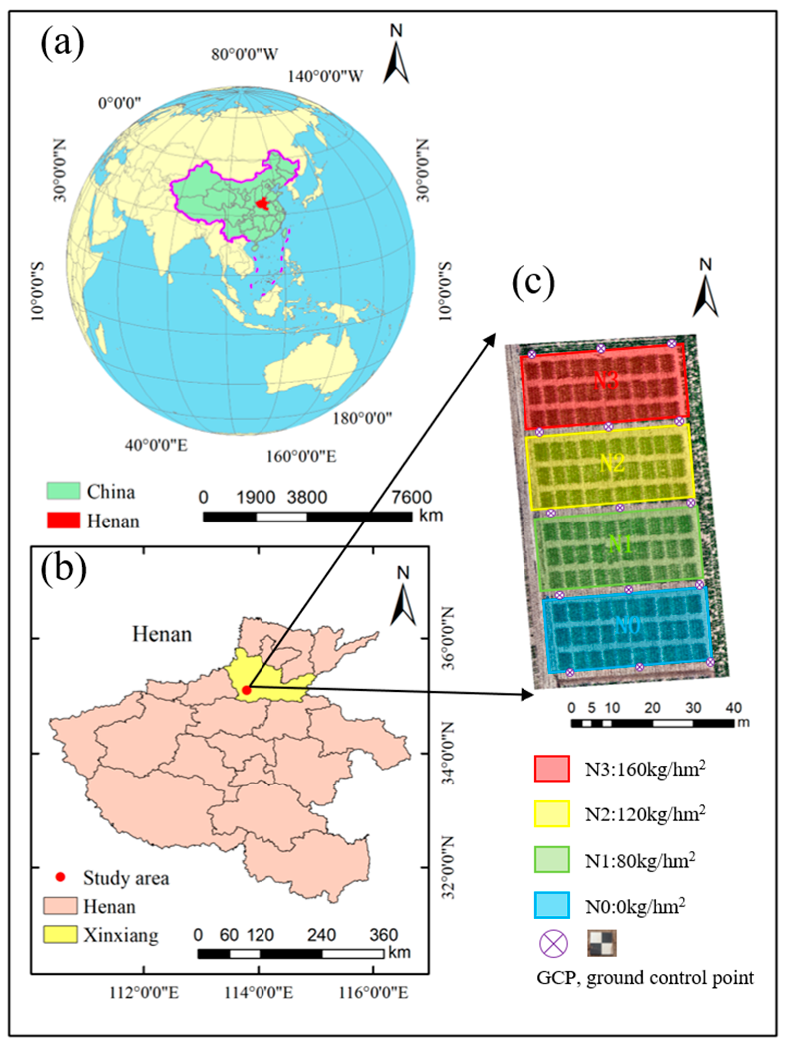
2.1. Study Area

The study area is located at the Xinxiang Comprehensive Experimental Base of the Chinese Academy of Agricultural Sciences, Xinxiang County, Henan Province, China (113°45′42″E, 35°08′05″N, Figure 1). The study area is located in the Yellow River Basin, with fertile soil and ample sunlight. It experiences a warm temperate continental monsoon climate, with an average annual temperature of 14.3 °C and an average temperature difference of 16.5 °C. The average annual precipitation is approximately 560.6 mm, making it suitable for the growth of summer maize. The experiment was conducted from June to September 2023 and involved a total of ten maize varieties. Four different nitrogen fertilizer treatments were applied: N0 (0 kg/hm²), N1 (80 kg/hm²), N2 (120 kg/hm²), and N3 (160 kg/hm²). Each treatment was replicated three times, and each plot had dimensions of 2 m × 4 m, resulting in a total of 120 plots. The experiment was conducted in the field with manual weed control. When the soil moisture reached the lower limit of irrigation control, irrigation was carried out. The upper limit of irrigation was the field capacity, and irrigation was conducted using sprinkler irrigation. The 3D coordinates of the Ground Control Points were determined using a S3IISE (Guangzhou STONEX Mapping Technology Co., Ltd., Guangzhou, China) geodetic GNSS receiver.

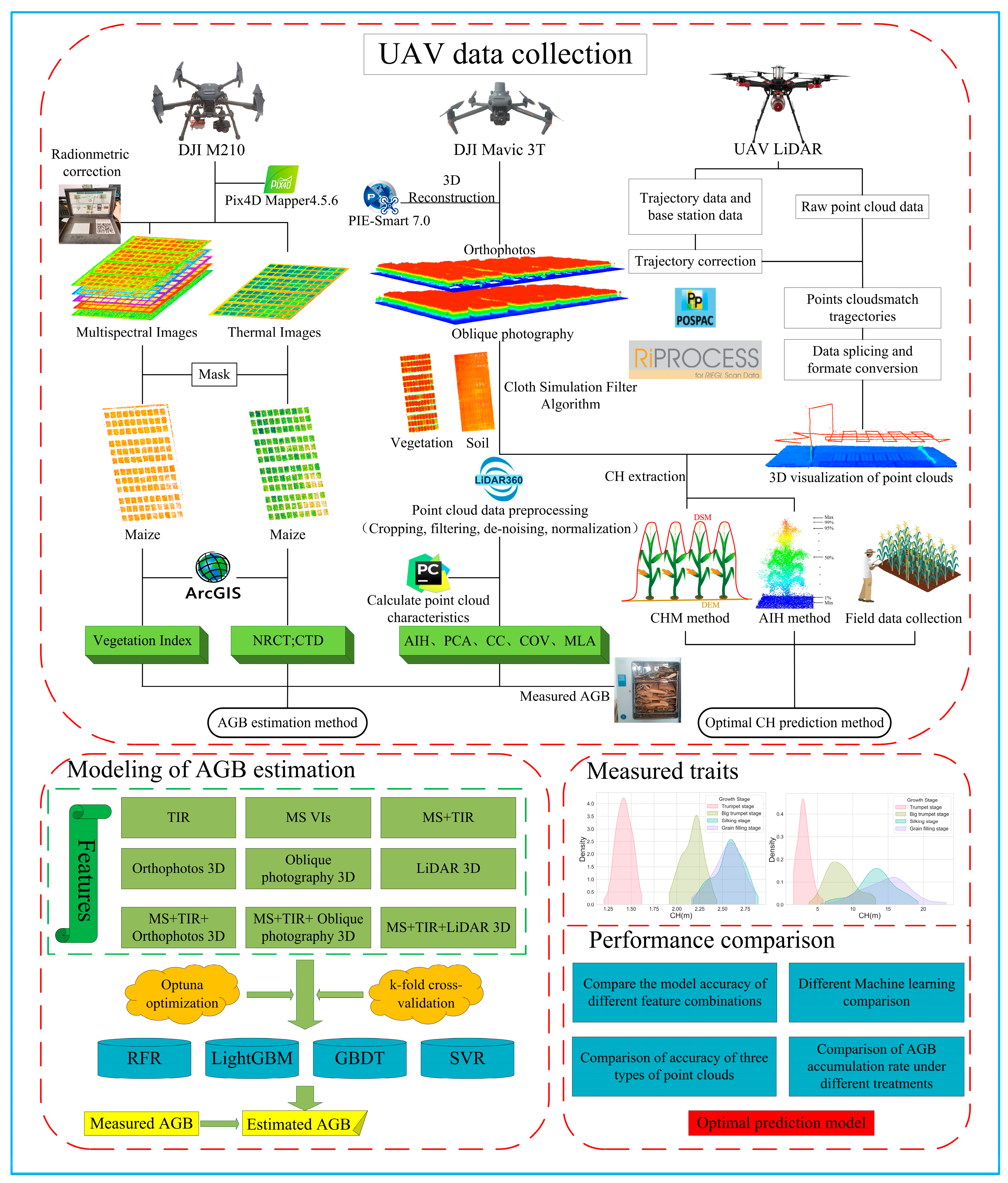
2.2. Data Collection and Feature Extraction

2.2.1. Ground Data Acquisition

The experiment was carried out across various growth stages of summer maize, including the trumpet stage, the big trumpet stage, the silking stage, and the grain-filling stage. The primary data collected comprised summer maize CH and AGB data. The CH was measured precisely using a tower ruler with millimeter accuracy. Within each experiment, three random measurements of maize canopy heights were taken to establish ground truth values. To obtain accurate maize AGB data, two representative maize plants were randomly selected from each plot as samples. These fresh samples were immediately placed in an electrically heated forced-air drying oven at 105 °C for 30 min to arrest enzymatic activity. Subsequently, they were dried at 75 °C until constant weight (approximately 24–48 h). The dried samples were then weighed to determine their dry weight, and these measurements were recorded. Finally, the AGB of summer maize at the field scale (t/hm²) was calculated by leveraging the dry weight of the samples and the planting density.

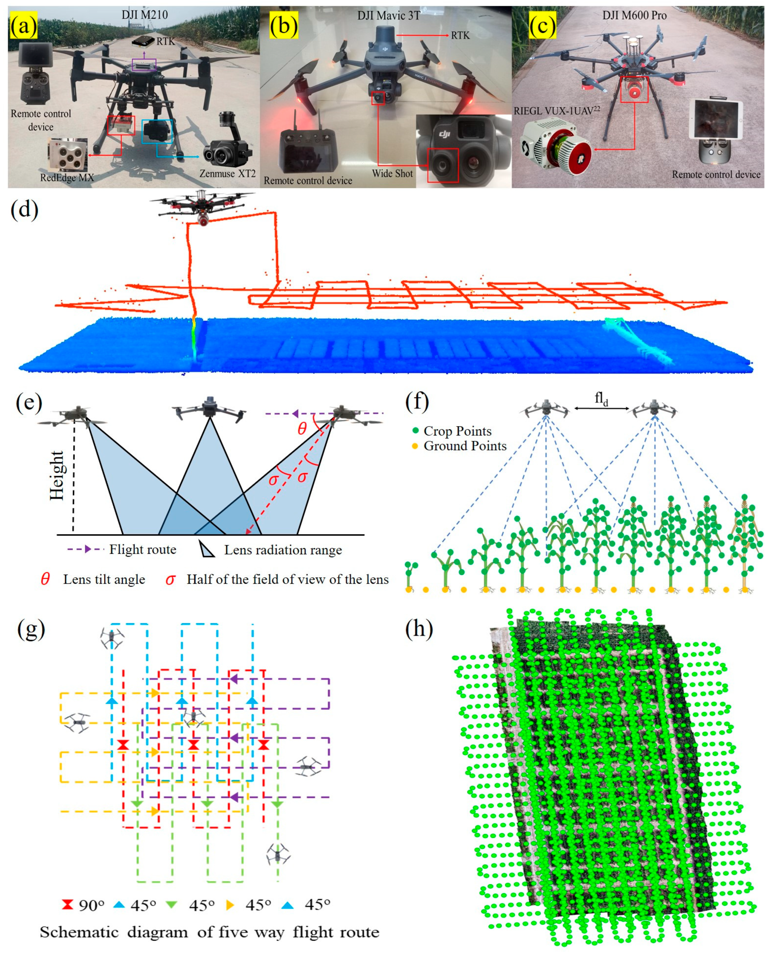
2.2.2. UAV Data Acquisition

In this study, data acquisition for multispectral and thermal infrared imagery was performed using the DJI M210 UAV (SZ DJI Technology Co., Shenzhen, China) equipped with a RedEdge MX multispectral camera and a Zenmuse XT2 thermal sensor (Figure 2). To mitigate the effects of solar zenith angle variations, image data were collected between 11:30 AM and 12:30 PM Beijing time. The RedEdge-MX sensor is a five-band multispectral camera, with bands centered at blue (475 ± 20 nm), green (560 ± 20 nm), red (668 ± 10 nm), red edge (717 ± 10 nm), and near-infrared (840 ± 40 nm). The Zenmuse XT2 thermal sensor has a resolution of 640 × 512, a sensor size of 10.88 mm × 8.704 mm, and a focal length of 19 mm. Flight paths were planned using the DJI Pilot 2 software (SZ DJI Technology Co., Shenzhen, China) with an equal time-interval capture mode. The UAV camera was kept perpendicular to the ground, with a flight altitude set at 30 m. The forward overlap rate was set to 85%, and the side overlap rate was set to 80%. The number of single-band or thermal infrared photos taken during a single flight was 644, with a GSD of 5.86 cm/pixel.

To obtain 3D point cloud data, three types of data were collected: nadir photography, oblique photography, and LiDAR. Nadir photography and oblique photography were captured using the wide angle lens of the DJI Mavic 3T UAV, which has a sensor size of 6.4 mm × 4.8 mm, a resolution of 4000 × 3000, an equivalent focal length of 24 mm, and effective pixels of 48 megapixels. Oblique photogrammetry was conducted through multiple flights over the same area. Five flight paths were set up to simulate a five-camera setup, capturing images in the downward, forward, backward, leftward, and rightward directions. The flight altitude was set to 12 m, with a forward overlap rate of 85% and a side overlap rate of 80%, to achieve 3D modeling. The GSD for a single flight was 0.33 cm/pixel, and the oblique GSD was 0.46 cm/pixel. The number of images and point cloud density collected during flight are shown in

Table 1. Number and density of different types of point clouds.

Data	Growth Stage	Number of Images	Point Number	Maximum Density (Points/m2)	Average Density (Points/m2)
Nadir photography	Trumpet	279	14145676	16,152	5206.36
	Big trumpet	306	11727280	10,404	4278.47
	Silking	308	5767643	7006	2133.79
	Grain-filling	305	9870493	9411	3705.14
Oblique photography	Trumpet	1534	50155628	44,924	18,365.3
	Big trumpet	1526	45023633	48,450	16,207.2
	Silking	1774	46439446	69,036	17,060.8
	Grain-filling	1772	43336920	48,793	15,770.3
LiDAR	Trumpet	/	3471345	3266	1260.93
	Big trumpet	/	2877150	3510	1037.93
	Silking	/	3488299	4224	1366.89
	Grain-filling	/	4522743	4579	1636.9

. LiDAR data collection was performed using the RIEGL VUX-1HA²² mounted on a DJI M600 UAV, with UAV positioning provided by FindCM, at the flight altitude of 20 m (Figure 2). The RIEGL VUX-1HA²² is equipped with a high-speed rotating mirror and captures uniformly distributed point cloud data through near-infrared laser beams and rapid line scanning, enabling high-precision laser measurements. Its laser emission frequency reaches up to 1800 kHz, with a scan speed ranging from 10 to 250 revolutions per second. The field of view angle is 360^o, the accuracy is 10 mm, the repeatability is 3 mm, and the laser spot size is 25 mm × 50 m.

2.2.3. Image Processing and Data Extraction

After obtaining the multispectral and thermal infrared image data from the UAV, Pix4D 4.5.6 (Pix4D, Lausanne, Switzerland) was utilized for stitching together multispectral and thermal infrared images, thus producing orthophoto maps. During the stitching process of the multispectral images, the software-processing options were set to use the “Rapid” option for initial processing. For radiometric processing and calibration, calibration panel images were imported for radiometric correction. To stitch the thermal infrared images, the temperature grayscale map was generated by selecting the corresponding option in the index calculator. To mitigate the soil’s influence on vegetation reflectance, kernel-normalized-difference vegetation indexes (kNDVIs) corresponding to each growth stage were calculated. Utilizing the natural breaks method to determine the optimal threshold point between maize and soil, threshold segmentation was executed, yielding a vector mask of summer maize used to mask the original images. ArcGIS 10.8 (ESRI, Redlands, CA, USA) was employed to draw polygons’ shapefile over reflectance images of different bands, thus extracting average values of each area as features. Nine vegetation index features were constructed based on acquired multispectral images and prior research (

Table 2. Vegetation indices selected in this study.

Features	Formula	Reference
Kernel-normalized-difference vegetation index (kNDVI)	$\tan \mathrm{h}\left({\left({\displaystyle \frac{\mathrm{NIR}-\mathrm{R}}{2\mathsf{\sigma }}}\right)}^2\right)$	[30]
Vegetation index green (VIG)	$\left(\mathrm{G}-\mathrm{R}\right)/\left(\mathrm{G}+\mathrm{R}\right)$	[31]
Ratio vegetation index (RVI)	$\mathrm{NIR}/\mathrm{R}$	[6]
Green–red-normalized-difference vegetation index (GRNDVI)	$\left(\mathrm{NIR}-\left(\mathrm{G}+\mathrm{R}\right)\right)/\left(\mathrm{NIR}+\left(\mathrm{G}+\mathrm{R}\right)\right)$	[32]
Renormalized-difference vegetation index—red edge (RDVI-REG)	$(\mathrm{NIR}-\mathrm{EDGE})/\sqrt{(\mathrm{NIR}+\mathrm{EDGE})}$	[33]
Optimization of soil regulatory vegetation index (OSAVI)	$1.16\left(\mathrm{NIR}-\mathrm{R}\right)/\left(\mathrm{NIR}+\mathrm{R}+0.16\right)$	[34]
Red green blue vegetation index (RGBVI)	$\left({\mathrm{G}}^2-\mathrm{B}\ast \mathrm{R}\right)/\left({\mathrm{G}}^2+\mathrm{B}\ast \mathrm{R}\right)$	[35]
Visible-band-difference vegetation index (VARI)	$\left(\mathrm{G}-\mathrm{R}\right)/\left(\mathrm{G}+\mathrm{R}-\mathrm{B}\right)$	[36]
Wide dynamic range vegetation index (WDRVI)	$\left(\mathrm{NIR}-\mathrm{R}\right)/\left(\mathrm{NIR}+\mathrm{R}\right)$	[28]

$\alpha$ = 0.667, $\sigma$ = 0.5 (NIR + R). R: red band reflectivity; G: green band reflectivity; B: blue band reflectivity; NIR: near-infrared band reflectivity; EDGE: red edge band reflectivity.

).

Nadir photography and oblique photography images were imported into PIE-Smart 7.0 (http://www.piesat.cn, accessed on 2 January 2024) for 3D model reconstruction, generating LAS-format point cloud data. After importing image information, we set the feature point density to high and the number of feature points to 5000. In image alignment, we set the adjustment accuracy to high and the filter adjustment times to 3. We matched the connection point accuracy to 1 pixel selected connection point thinning. After image alignment was complete, we performed Ground Control Points editing for photogrammetric camera optimization (

Table 3. Error metrics after image orientation using Ground Control Points (GCPs) in oblique photogrammetry.

Growth Stage	dx (m)	dy (m)	dz (m)	3D Error (m)	Vertical Error (m)	Horizontal Error (m)
Trumpet stage	0.057	0.056	0.084	0.116	0.084	0.080
Big trumpet stage	0.059	0.058	0.057	0.101	0.057	0.083
Silking stage	0.037	0.047	0.034	0.069	0.034	0.06
Grain-filling stage	0.062	0.053	0.070	0.108	0.070	0.082

). Afterward, we performed 3D processing. In reconstruction parameters, we set the resolution level to high and chose to generate the point cloud in .las format. LiDAR data preprocessing is relatively complex. To obtain accurate point cloud data of summer maize, a precise trajectory calculation was conducted using POSPac (Applanix Co., Richmond Hill, ON, Canada). The original laser point cloud was preprocessed using the PiPROCESS (PEIGL Co., Vienna, Austria) point cloud processing software. This mainly involves waveform processing of the original LiDAR data based on the precise trajectory of the UAV, the instrument installation orientation, and the sightline adjustment parameters, converting LiDAR scanning data to the precise trajectory coordinates of the UAV, matching LiDAR data with trajectory data, etc. Finally, we exported 3D LiDAR data. Green Valley International LiDAR360 5.2 software (GreenValley, Beijing, China) was utilized for preprocessing different point cloud data types. A random forest supervised classification algorithm was employed for point cloud classification, followed by certain operations, such as clipping, filtering, and denoising, to extract summer maize structural features. The cloth simulation filtering (CSF) algorithm was utilized to distinguish ground and non-ground points in point cloud data. The CSF algorithm circumvents the intricate calculations found in slope-based, mathematical morphological, and surface-based models, making it suitable for diverse geographical areas with fewer parameters. Based on three types of point cloud data, various structural features were extracted from their 3D structures, including canopy occupation volume (COV), projected canopy area (PCA), canopy cover (CC), mean leaf angle (MLA), and AIH. The calculation of COV involves a grid-based discretization of the model, which entails a statistical analysis of the height difference between the highest and lowest points within each grid cell. This height difference is multiplied by the grid cell size to obtain the volume of each grid cell. The total vegetation volume is then obtained by summing the volumes of all grid cells. The height distribution map of different types of point cloud data is shown in Figure 3.

2.2.4. Canopy Temperature Information

Through segmentation statistics, normalized relative canopy temperature (NRCT) and canopy temperature depression (CTD, °C) were obtained from UAV thermal infrared images for estimating aboveground biomass canopy temperature information, with the following formulas:

$$\mathrm{N}\mathrm{R}\mathrm{C}\mathrm{T}={\displaystyle \frac{{\mathrm{T}}_{\mathrm{i}}-{\mathrm{T}}_{\mathrm{m}\mathrm{i}\mathrm{n}}}{{\mathrm{T}}_{\mathrm{m}\mathrm{a}\mathrm{x}}-{\mathrm{T}}_{\mathrm{m}\mathrm{i}\mathrm{n}}}}$$

(1)

$$\mathrm{C}\mathrm{T}\mathrm{D}={\mathrm{T}}_{\mathrm{i}}{-\mathrm{T}}_{\mathrm{a}}$$

(2)

${\mathrm{T}}_{\mathrm{i}}$ is the canopy temperature of the ${\mathrm{i}}_{\mathrm{t}\mathrm{h}}$ pixel, ${\mathrm{T}}_{\mathrm{m}\mathrm{a}\mathrm{x}}$ is the maximum temperature in the field experiment, ${\mathrm{T}}_{\mathrm{m}\mathrm{i}\mathrm{n}}$ is the minimum temperature in the field experiment, and ${\mathrm{T}}_{\mathrm{a}}$ is the air temperature.

2.3. AGB Model Construction

To identify the best model for estimating maize AGB, four machine-learning algorithms were selected for comparative analysis. Machine-learning algorithms are adept at handling complex nonlinear relationships between remote-sensing variables and crop biophysical/biochemical parameters. Compared to traditional regression algorithms, machine-learning techniques exhibit superior performance in regression predictions involving multiple input variables. This study constructed models for estimating maize AGB by extracting features from multi-source remote-sensing data.

SVR is grounded in the Vapnik–Chervonenkis dimension theory and the principle of structural risk minimization. It addresses the problem of function approximation, and it is a small-sample statistical theory formed on the basis of ordered risk minimization. SVR is effective in mitigating overfitting to some extent, demonstrating good stability and universality. Currently, SVR is widely applied in computer vision and data analytics [37]. This approach fits the sample data while alleviating issues, such as overfitting and underfitting, during the training process. The SVR model uses the radial-basis function kernel, with optimal parameters for C and gamma determined using the Optuna algorithm.

GBDT is a powerful boosting ensemble learning algorithm that employes decision trees or regression trees as base learners for solving classification or regression problems. To iteratively update the new learner using the gradient descent algorithm [38], the base learners in GBDT are typically classification and regression trees (CARTs). The objective is to minimize the discrepancy between the true values and the predicted values, often using the mean squared error as the loss function. In each iteration, decision trees are trained to predict the residuals of the current model. Each subsequent tree attempts to correct the residuals of the previous one, thereby continuously improving the overall prediction accuracy of the model. This iterative training process enhances the predictive capability of GBDT. GBDT is renowned for its strong predictive performance, high flexibility, robustness, and interpretability. However, it performs poorly with high-dimensional sparse data compared to other algorithms, like SVR, and it is difficult to train in parallel.

LightGBM is a boosting ensemble learning algorithm within the gradient-boosting framework designed for efficient handling of large-scale datasets and high-dimensional features [28]. Essentially, it integrates weak learners, with each iteration attempting to reduce the gradient of the loss function. LightGBM operates within the framework of GBDT, optimizing the process of finding split points for base learner decision trees, as well as the way the trees grow. Using the histogram algorithm accelerates the process of finding split points, reduces memory consumption, and employs a leaf-wise leaf growth strategy with depth limits to enhance the accuracy of base learners, resulting in a more efficient generation of decision trees. Subsequently, innovative techniques, like gradient-based one-side sampling (GOSS) and exclusive feature bundling (EFB), were introduced to enhance model training speed and accuracy. It demonstrates outstanding performance in managing high-dimensional data and nonlinear problems, typically outperforming other gradient-boosting frameworks in predictive accuracy. However, it exhibits sensitivity to noise and outliers, rendering parameter-tuning challenging.

The RFR algorithm, proposed by Leo Breiman and Adele Cutler, is a machine-learning method widely utilized for both classification and regression tasks [39]. As a prominent example of ensemble learning algorithms within the bagging framework, RFR accomplishes regression tasks by constructing multiple decision trees and integrating their predictions. In RFR, each decision tree is independently trained on randomly selected subsets of the data, effectively mitigating the risk of overfitting. The final prediction result is obtained by averaging or weighted-averaging the predictions of these decision trees. The hyperparameters set in the RFR algorithm include n_estimators, max_features, max_depth, min_samples_split, and min_samples_leaf. These hyperparameters were optimized using the Optuna algorithm, resulting in an average number of 30 trees throughout the entire growth cycle. RFR demonstrates strong robustness and generalization capabilities, particularly when handling high-dimensional data.

Hyperparameter tuning is crucial for optimizing different machine-learning algorithms. Complex models with numerous parameters are prone to overfitting, and overfitting is likely to occur. Meanwhile, simpler, shallow models struggle to fit complex nonlinear data well and are prone to underfitting. Optuna is an open-source hyperparameter optimization (HPO) framework designed to be compatible with various machine-learning frameworks, thus enabling comprehensive exploration of hyperparameter search spaces. In this study, we utilized sequential model-based optimization (SMBO) through Optuna to efficiently search for optimal hyperparameters. Optuna continuously explores the parameter space by minimizing the value of the cost function, aiming to identify the best hyperparameter combinations. The advantages of Optuna include efficiency, ease of use, scalability, and customizability. In this study, the RFR, LightGBM, GBDT, and SVR regression models were built, and the Optuna framework was integrated to optimize the estimation models.

2.4. Evaluation Metrics

The model accuracy is evaluated using three metrics: the coefficient of determination (R²), the root mean square error (RMSE), and the normalized root mean square error (nRMSE). An R² value closer to 1 indicates a better fit of the model. Lower values of RMSE and nRMSE signify better predictive performance of the model.

$${\mathrm{R}}^2={\displaystyle \frac{{(\sum _{\mathrm{i}=1}^{\mathrm{n}}{\mathrm{y}}_{\mathrm{i}}-\overline{\mathrm{y}})}^2}{{(\sum _{\mathrm{i}=1}^{\mathrm{n}}{\mathrm{x}}_{\mathrm{i}}-\overline{\mathrm{y}})}^2}}$$

(3)

$$\mathrm{RMSE}=\sqrt{{\displaystyle \frac{\sum _{\mathrm{i}=1,\mathrm{j}=1}^{\mathrm{n}}{({\mathrm{x}}_{\mathrm{i}}-{\mathrm{y}}_{\mathrm{j}})}^2}{\mathrm{n}}}}$$

(4)

$$\mathrm{nRMSE}={\displaystyle \frac{\mathrm{RMSE}}{\overline{\mathrm{y}}}}\times 100\%$$

(5)

In the formula, ${\mathrm{x}}_{\mathrm{i}}$ represents the actual measured value of maize aboveground biomass, ${\mathrm{y}}_{\mathrm{i}}$ represents the estimated value of maize aboveground biomass, i and j are sample identifiers, n is the number of samples, and $\overline{\mathrm{y}}$ is the mean value of the actual measurements.

The experimental workflow of this study is depicted in Figure 4. Features were extracted from nadir photography, oblique photography, LiDAR, multispectral, and thermal infrared imagery. Concurrently, measured values of maize CH and AGB were collected as the target variables. We compared the performance of the CHM and AIH methods in extracting CH to find the optimal estimation method. By constructing maize AGB estimation models through multi-feature coupling, this study aims to quickly and accurately monitor crop growth, laying the foundation for achieving smart agriculture.

3. Results

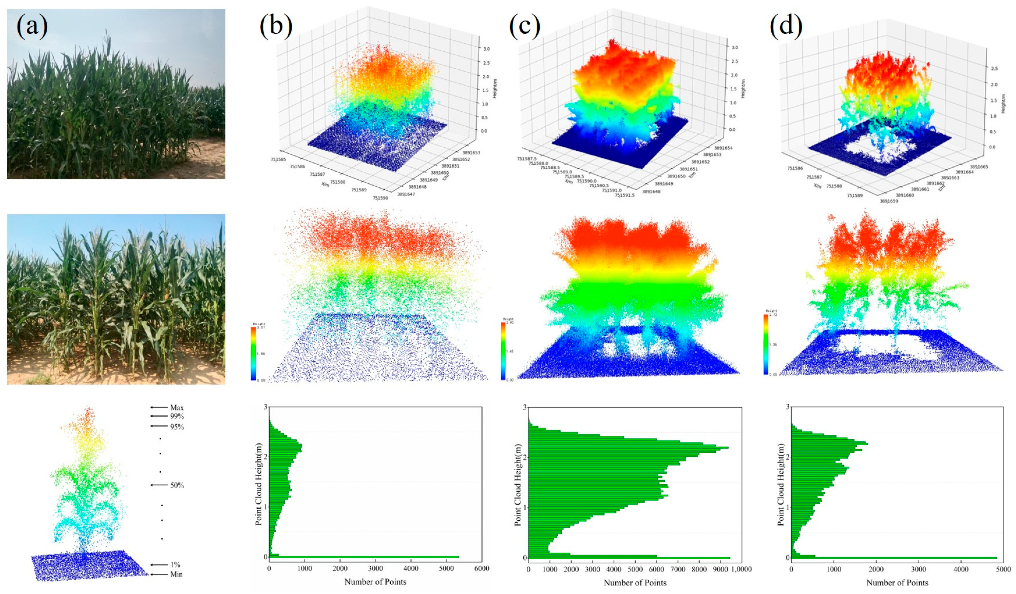
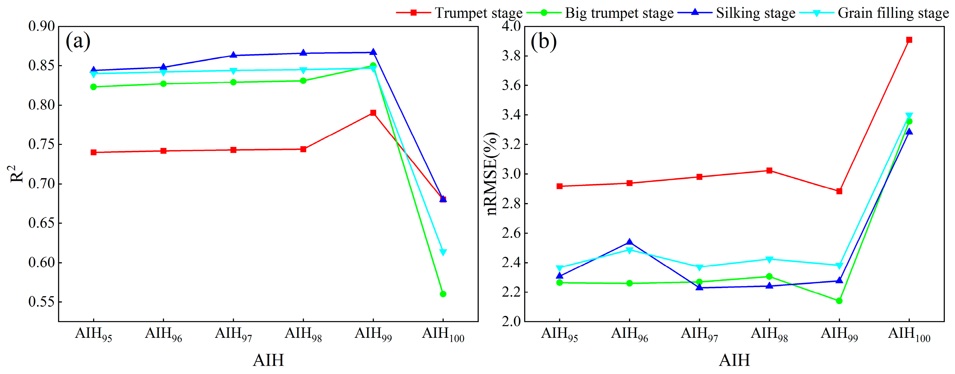
3.1. Extraction of Maize Crop Height at Various Growth Stages

The trend in maize CH initially exhibited rapid growth, followed by gradual stabilization (Figure 5). From the trumpet stage to the big trumpet stage, maize showed rapid growth and development. Upon entering the silking stage, the rate of height increase slowed, with CH slightly decreasing towards the grain-filling stage. In this study, linear regression analysis was applied between the average height of maize extracted from the CHM and the ground observations, with the regression accuracy depicted in Figure 6. The results showed that the accuracy during the big trumpet and silking stages was higher than in the other two growth stages. However, compared to the manually measured height, the extracted corn height showed varying degrees of underestimation. Specifically, at the big trumpet stage, R² peaked at its maximum value of 0.68, and the RMSE reached its minimum value of 6.79 cm.

The higher AIH percentile serves as an intuitive reflection of CH. To determine the optimal AIH percentile for estimating CH, this study extracted various AIH percentile values exceeding the AIH₉₅ using LiDAR point cloud data. It was observed that as AIH gradually changed, the accuracy of CH estimation initially improved and then decreased. At the AIH₉₉ threshold, the estimation accuracy of CH during various growth stages reached a relatively high level, with the nRMSE being relatively low, ranging between 2.14% and 2.88% (Figure 7). Thus, selecting the AIH₉₉ threshold is deemed more appropriate for estimating CH when extracting point cloud data based on the AIH method.

The 99% AIH from point clouds generated by LiDAR, oblique photography, and nadir photography maps was selected as the upper limit. The extracted CH (mean value) was then compared with the manually measured maize CH (Figure 8). The results showed that height extraction based on LiDAR data yielded the highest estimation accuracy, with R² consistently exceeding 0.75 and RMSE within 10 cm. Using oblique photography point cloud data, the R² for extracting maize height ranged from 0.74 to 0.80, while the RMSE ranged from 4.21 to 7.24 cm. During various growth stages, both oblique photography and nadir photography exhibited varying degrees of underestimation in CH compared to LiDAR point cloud data. The underestimation phenomenon was weakest during the silking stage, with the smallest differences, and most pronounced during the trumpet stage. Based on the estimation accuracy of the three sensors, the performance ranking was LiDAR > oblique photography > nadir photography. The LiDAR sensor performed the best in extracting maize CH, providing a valuable reference for large-scale CH estimation.

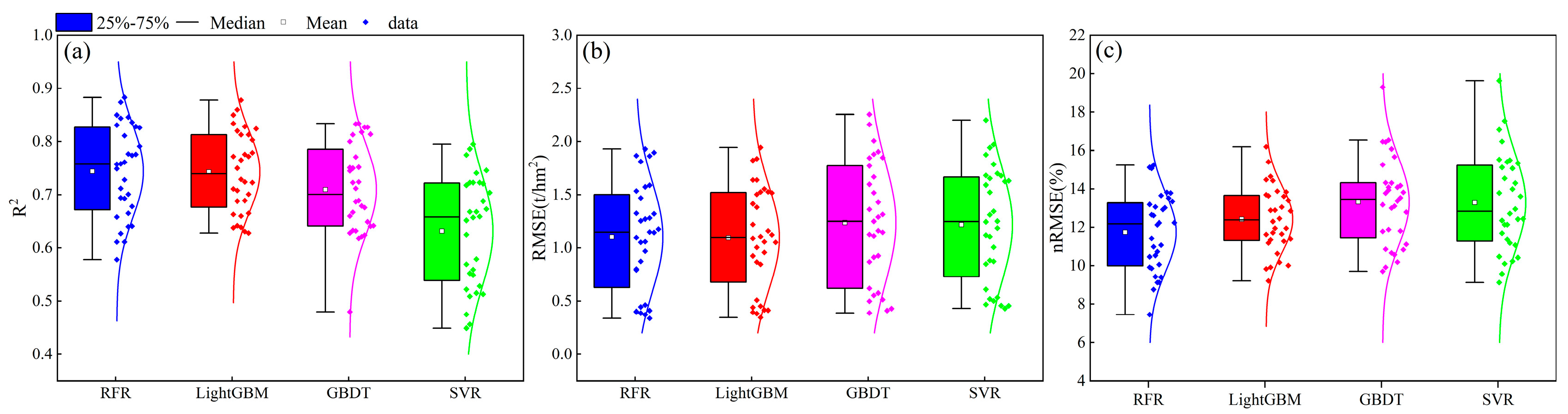
3.2. AGB Estimation for Entire Growth Cycle

This study evaluated the accuracy of maize AGB estimation throughout the entire growth cycle using multi-source remote-sensing data from UAVs. The results indicated that estimations using MS, oblique photography 3D, or LiDAR 3D data all performed well, whereas the estimation based on the TIR sensor was the least accurate (

Table 4. The accuracy of maize AGB estimation across different sensor combinations and machine-learning algorithms during the entire growth cycle.

Data Type	RFR		LightGBM		GBDT		SVR
	R2	nRMSE (%)	R2	nRMSE (%)	R2	nRMSE (%)	R2	nRMSE (%)
TIR	0.797	24.17	0.809	12.66	0.780	13.57	0.734	28.53
MS	0.850	19.50	0.857	10.76	0.852	9.299	0.836	20.98
MS+TIR	0.884	18.42	0.881	9.78	0.866	10.51	0.841	21.96
Nadir photography 3D	0.853	20.48	0.863	10.47	0.846	10.71	0.829	21.02
Oblique photography 3D	0.889	19.38	0.900	8.22	0.880	8.990	0.858	21.18
LiDAR 3D	0.879	17.79	0.899	8.14	0.873	9.194	0.860	19.11
MS+TIR+Nadir photography 3D	0.905	15.75	0.915	7.707	0.884	10.38	0.863	21.49
MS+TIR+oblique photography 3D	0.929	15.39	0.939	6.477	0.898	8.514	0.880	18.88
MS+TIR+LiDAR 3D	0.912	15.14	0.916	7.595	0.902	8.169	0.895	17.83

). For the MS sensor, the R² ranged from 0.836 to 0.857 and the RMSE ranged from 1.867 to 2.008 t/hm². Oblique photography slightly outperformed LiDAR in estimating maize AGB. The R² for AGB estimation based on oblique photography ranged from 0.858 to 0.900, and the RMSE was between 1.636 and 1.953 t/hm². Combining MS, TIR, and point cloud data resulted in greater estimation performance. The accuracy of maize AGB estimation using MS+TIR+oblique photography 3D features was comparable to that of MS+TIR+LiDAR 3D, with the oblique photography combination performing slightly better than the LiDAR combination. Using the RFR, LightGBM, GBDT, and SVR algorithms, the R² for the oblique photography combination was 0.929, 0.939, 0.898, and 0.880, respectively, with a corresponding RMSE of 1.432, 1.326, 1.631, and 1.766 t/hm².

3.3. AGB Estimation for Different Growth Stages

Different algorithms exhibit varying estimation accuracies at different growth stages of maize. The mean R² for the SVR algorithm is 0.63, with a mean RMSE of 1.22 t/hm². For the GBDT algorithm, the mean R² is 0.71, with a mean RMSE of 1.23 t/hm². The mean R² for the RFR and LightGBM algorithms are 0.744 and 0.743, with mean RMSEs of 1.104 t/hm² and 1.096 t/hm², respectively. These results suggest that the adopted LightGBM and RFR ensemble learning algorithms have a significant advantage in estimating AGB (

Table A1. Comparison of AGB estimation accuracy for different maize growth stages and algorithms.

Growth Stage	Features	RFR		LightGBM		GBDT		SVR
		R2	nRMSE (%)	R2	nRMSE (%)	R2	nRMSE (%)	R2	nRMSE (%)
Trumpet stage	MS	0.757	13.19	0.711	13.69	0.652	15.52	0.628	16.45
	MS+TIR	0.761	13.06	0.765	12.88	0.667	15.25	0.643	16.26
	nadir photography 3D	0.611	15.12	0.638	15.40	0.633	14.32	0.509	19.64
	Oblique photography 3D	0.694	12.92	0.724	12.45	0.689	11.79	0.659	16.46
	LiDAR 3D	0.578	15.23	0.660	13.61	0.480	19.30	0.515	17.54
	MS+TIR+nadir photography 3D	0.776	13.34	0.779	11.95	0.712	14.17	0.688	15.07
	MS+TIR+oblique photography 3D	0.811	12.24	0.820	11.27	0.771	12.79	0.723	14.30
	MS+TIR+LiDAR 3D	0.828	11.07	0.813	11.39	0.752	11.81	0.721	15.33
Big trumpet stage	MS	0.758	12.65	0.772	14.48	0.745	13.17	0.668	13.79
	MS+TIR	0.777	12.13	0.776	12.30	0.718	10.47	0.751	13.00
	nadir photography 3D	0.627	15.07	0.642	14.65	0.632	14.09	0.475	15.12
	Oblique photography 3D	0.693	13.02	0.701	13.05	0.679	13.53	0.549	13.99
	LiDAR 3D	0.701	13.79	0.689	11.72	0.676	15.67	0.579	15.49
	MS+TIR+nadir photography 3D	0.831	9.85	0.834	10.62	0.800	9.70	0.723	12.44
	MS+TIR+ Oblique photography 3D	0.846	10.06	0.813	11.95	0.833	10.66	0.741	11.18
	MS+TIR+LiDAR 3D	0.874	9.13	0.803	12.85	0.827	10.83	0.746	11.07
Silking stage	MS	0.749	10.46	0.750	11.62	0.723	13.78	0.657	12.35
	MS+TIR	0.774	9.914	0.772	11.18	0.750	13.10	0.668	12.14
	nadir photography 3D	0.658	11.42	0.639	12.89	0.618	16.44	0.456	14.55
	Oblique photography 3D	0.640	13.82	0.631	14.43	0.624	16.08	0.552	12.95
	LiDAR 3D	0.665	10.98	0.665	13.84	0.641	14.09	0.528	12.42
	MS+TIR+Nadir photography 3D	0.844	8.75	0.850	10.17	0.813	10.85	0.775	10.10
	MS+TIR+oblique photography 3D	0.850	9.43	0.860	9.83	0.834	10.56	0.786	9.12
	MS+TIR+LiDAR 3D	0.883	7.45	0.878	9.20	0.827	11.11	0.795	9.57
Grain-filling stage	MS	0.712	12.61	0.708	13.63	0.660	13.94	0.522	12.14
	MS+TIR	0.728	12.23	0.729	11.35	0.687	13.37	0.569	12.71
	nadir photography 3D	0.611	13.65	0.663	13.88	0.621	16.54	0.449	15.40
	Oblique photography 3D	0.641	13.51	0.688	16.19	0.649	14.31	0.559	11.69
	LiDAR 3D	0.678	10.53	0.628	13.39	0.642	13.82	0.513	13.61
	MS+TIR+Nadir photography 3D	0.791	10.73	0.723	11.65	0.724	11.88	0.673	11.37
	MS+TIR+Oblique photography 3D	0.836	9.117	0.828	10.01	0.818	10.19	0.723	10.23
	MS+TIR+LiDAR 3D	0.826	9.40	0.824	9.91	0.814	9.91	0.704	10.42

).

Figure 9 shows the accuracy performance of estimating maize AGB based on different features and their combinations. When estimating AGB based on a single sensor, it was found that the MS sensor has higher estimation accuracy, with a mean R² of 0.698 and a mean RMSE of 1.23 t/hm². Compared to nadir photography, the estimation accuracy is higher with oblique photogrammetry and LiDAR, with a mean R² of 0.648 and 0.615 and a mean RMSE of 1.28 t/hm² and 1.30 t/hm², respectively. Compared to using a single sensor alone, coupling multi-source sensor features can significantly improve the model’s accuracy and robustness. The estimation accuracy of MS+TIR demonstrates a certain improvement compared to a single sensor. Compared to the estimation accuracy of the MS sensor, the combination of MS+TIR+nadir photography 3D increased the mean R² by 0.07 and reduced the mean RMSE by 0.17 t/hm², the combination of MS+TIR+oblique photography 3D increased the mean R² by 0.11 and reduced the mean RMSE by 0.29 t/hm², and MS+TIR+LiDAR 3D increased the mean R² by 0.11 and reduced the mean RMSE by 0.27 t/hm².

Figure 10 depicts the performance of the RFR, LightGBM, and SVR algorithms in estimating AGB at different growth stages of maize. The results show that both RFR and LightGBM algorithms provide relatively accurate estimation results. Specifically, during the trumpet and silking stages, the LightGBM algorithm outperforms the RFR algorithm. Moreover, incorporating crop canopy structural features has a positive impact on improving estimation accuracy and mitigating spectral saturation. Both the MS+TIR+oblique photography 3D and MS+TIR+LiDAR 3D feature combinations can achieve accurate AGB estimation. During the big trumpet and silking stages, the MS+TIR+oblique photography 3D combination shows better estimation accuracy compared to the LiDAR combination.

The machine-learning algorithms used in this study performed well in estimating maize AGB (Figure 11). The R² for the RFR algorithm ranged from 0.578 to 0.883, with an RMSE between 0.338 and 1.930 t/hm² and an nRMSE between 7.45% and 15.23%. For the LightGBM algorithm, the R² ranged from 0.628 to 0.878, with an RMSE between 0.346 and 1.945 t/hm² and an nRMSE between 9.2% and 16.19%. The GBDT algorithm had an R² ranging from 0.48 to 0.834, with an RMSE between 0.389 and 2.257 t/hm² and an nRMSE between 9.7% and 19.3%. The SVR algorithm had an R² ranging from 0.449 to 0.795, with an RMSE between 0.430 and 2.203 and an nRMSE between 9.12% and 19.64%. Both the RFR and LightGBM algorithms demonstrated high accuracy in estimating maize AGB. The accuracy of the GBDT estimation was lower than that of LightGBM and RFR, with SVR having the poorest accuracy among the four machine-learning algorithms.

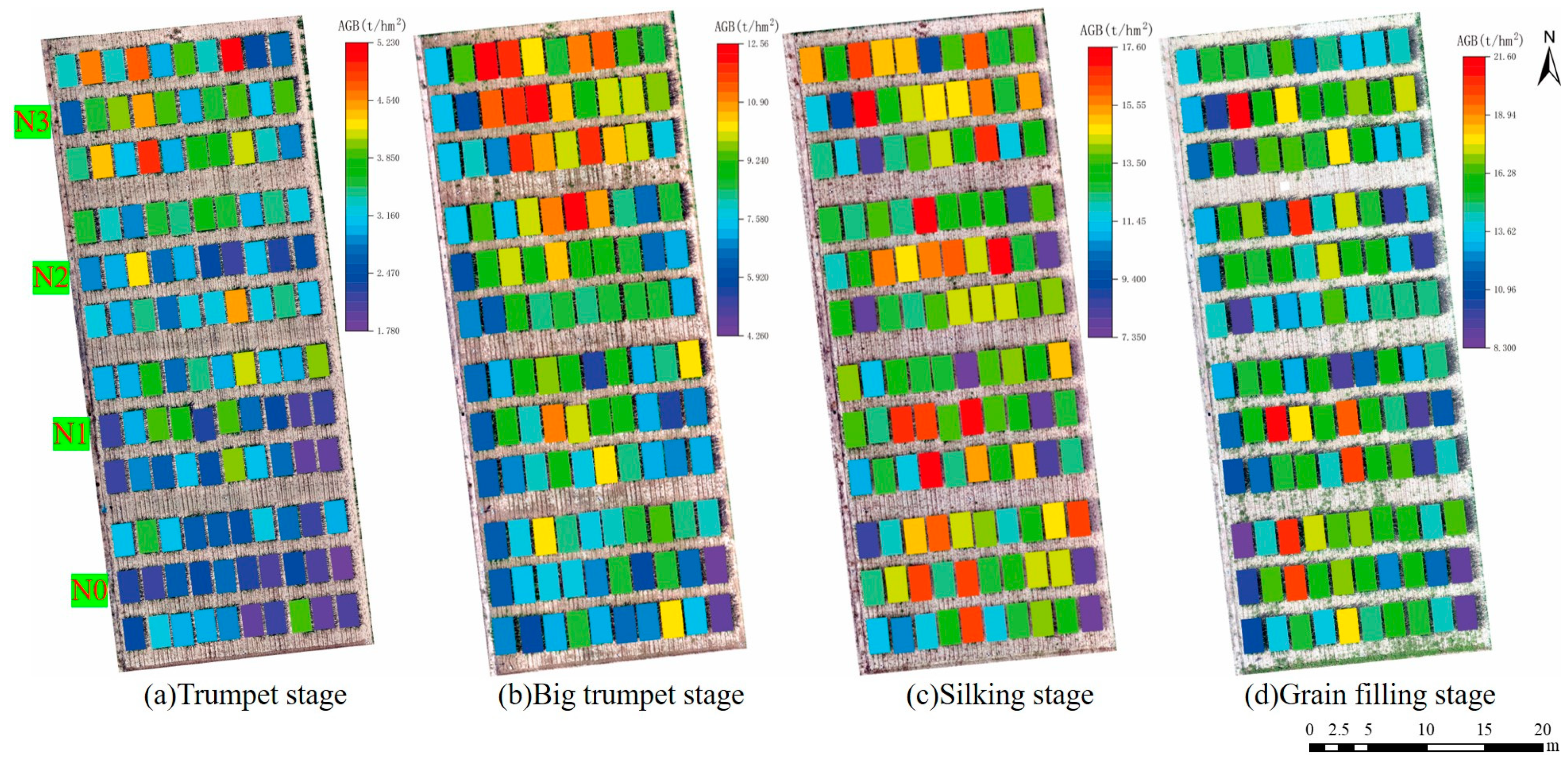
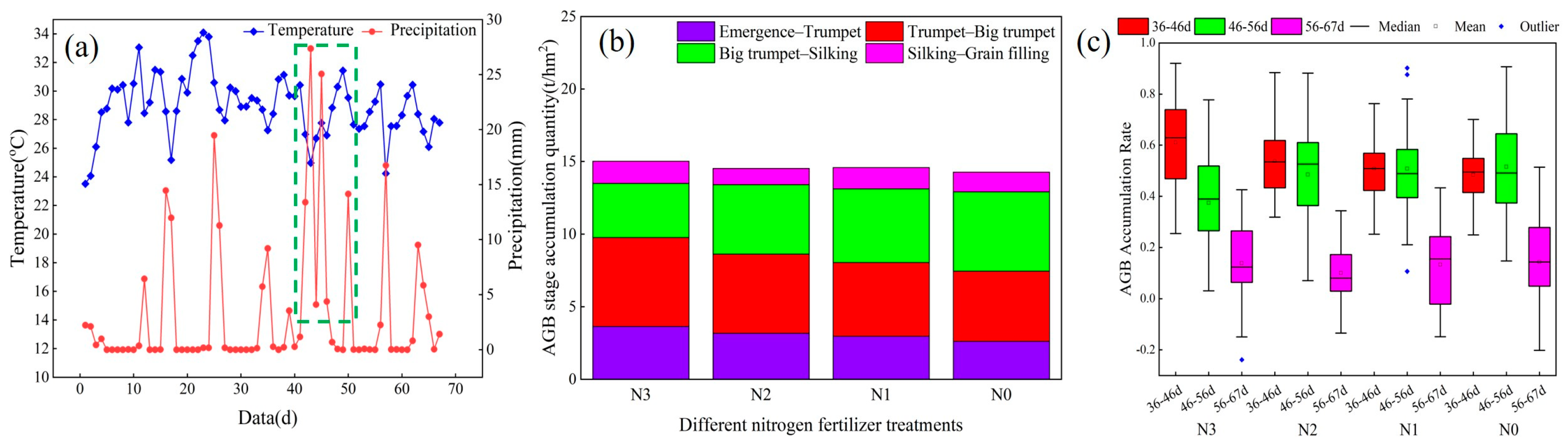
3.4. Spatiotemporal Distribution and Accumulation of AGB of Maize

Based on the estimation results from the RFR algorithm, the spatial distribution of AGB from the maize trumpet stage to the grain-filling stage in 2013 was mapped at the plot scale (Figure 12). The results indicate that as the growth stages of maize progress, AGB gradually increases and eventually stabilizes. As the amount of nitrogen fertilizer applied decreases gradually in the N3, N2, N1, and N0 treatments, the maize AGB shows a decreasing trend. The AGB distribution map clearly shows that the AGB of maize under the N3 and N2 treatments is higher than that under the N1 and N0 treatments. However, due to abundant rainfall in the later stages of maize growth, AGB increases rapidly, leading to reduced differences in AGB among the various nitrogen fertilizer treatments during the silking and grain-filling stages.

Figure 13 illustrates the stage-wise accumulation of maize AGB under various nitrogen treatments. Under the N3 treatment, maize AGB accumulates rapidly during the trumpet and big trumpet stages. Although the accumulation slows during the silking and grain-filling stages, the final accumulation is significantly higher compared to the other treatments, reaching 15.02 t/hm². In the initial two growth stages, the stage-wise accumulation of maize AGB decreases as the amount of nitrogen fertilizer is reduced, with the lowest accumulation observed under the N0 (no fertilizer) condition, at 7.44 t/hm². As the growth stages advance, several rainfalls exceeding 10 mm occur between the big trumpet stage and the grain-filling stage, leading to a rapid accumulation of maize AGB from the early big trumpet stage to the silking stage. This reduces the differences in AGB accumulation among the various treatments. Due to the influence of rainfall, the final accumulation of maize AGB under the N2 and N1 treatments is essentially the same. The results of the AGB accumulation rate indicated that as the growth period progressed, the accumulation rate gradually decreased, reaching its lowest point between 56 and 67 days. During 36–46 days, as the amount of nitrogen fertilizer decreased, the accumulation rate also decreased, with the lowest rate observed under the N0 treatment (no nitrogen fertilizer). The accumulation rates of maize were similar under the N2, N1, and N0 treatments during the 36–46-day and 46–56-day periods, with only minor differences.

4. Discussion

4.1. Comparison of Methods for Estimating Maize Crop Height

CH serves as a crucial indicator for assessing crop growth status and influencing light-use efficiency, making it a vital component of AGB. Accurate and rapid extraction of CH is essential for studying crop genetics and guiding agricultural production. Traditional methods for measuring CH typically involve manual field measurements. However, with the continuous development of UAV remote-sensing technology, new methods have emerged for closely monitoring CH changes over time using time-series data [40]. UAV-based CH-monitoring technology, relying on optical remote-sensing imagery, has reached a relatively mature stage. Nonetheless, it is significantly influenced by image quality and weather conditions. Additionally, in cases with high vegetation cover fraction, it may fail to accurately capture precise DEM information, thereby limiting the accuracy of the CHM. Chang et al. [18] utilized UAV imagery to generate DEM and DSM. Using the obtained CHM as the sorghum height, they successfully estimated growth curves for different sorghum varieties. The results indicated that the RMSE between the measured values and the predicted values was 0.33 m. With ongoing advancements in point cloud accuracy, the application of estimating CH based on 3D point clouds is gradually gaining traction. Wang et al. [19] compared and analyzed the accuracy of the AIH method and the mean method in extracting wheat CH, finding that the AIH method outperformed the mean method. The CH values extracted from the 90–100% AIH showed strong consistency with the measured values. The R² exhibited a trend of initially increasing and then decreasing with the risk of the percentile, reaching peak accuracy at the 99.5% AIH. This study further confirmed that the AIH method has greater accuracy compared to the CHM method through the comparison of various algorithms for extracting CH [40]. When monitoring CH using nadir photography, oblique photography, and LiDAR point clouds, it is observed that oblique photography and LiDAR point clouds exhibit comparable accuracy. However, LiDAR point cloud data provide slightly greater accuracy in estimating CH than oblique photography point clouds. This is likely because LiDAR is unaffected by lighting conditions, has robust penetration capabilities, and can precisely capture ground point cloud data [41]. Considering cost, constructing 3D point clouds based on oblique photography can, to some extent, replace LiDAR and is widely used in estimating crop structural parameters.

4.2. Impact of Data Sources and Modeling Algorithms on Biomass Estimation

Ensemble learning algorithms have been extensively applied in the agricultural field, yet the accuracy of AGB estimation varies significantly depending on the selected features and their combinations. Feature selection introduces uncertainty into AGB estimation accuracy [42]. Although UAV spectral images provide rich spectral features and vegetation indices, their limited penetration capability hinders the capture of vertical structural characteristics of crops like maize. Additionally, UAV spectral images often encounter issues, such as spectral saturation and poor sensitivity, when estimating crop AGB. Incorporating canopy structure characteristics can partially mitigate the problem of spectral saturation [3]. Therefore, this study extracted maize canopy structure characteristics using nadir photography, oblique photography, and LiDAR data to evaluate their effectiveness in enhancing model accuracy and robustness. Compared to maize AGB estimation using single-sensor remote-sensing data (TIR, MS, nadir photography 3D, oblique photography 3D, and LiDAR 3D), the fusion of multi-source remote-sensing data exhibited superior estimation performance across the entire growth cycle and at individual growth stages. This improvement is likely related to feature enhancement achieved through multi-source remote-sensing data fusion, consistent with the findings of Zhang et al. [43], who demonstrated efficient and accurate nitrogen-content monitoring through multi-source remote-sensing data fusion. TIR data provide information on crop canopy and soil temperatures, which are influenced by the crop’s genetic characteristics and the surrounding environment. Canopy temperature is closely related to leaf transpiration rates, crop organ growth, and starch synthesis [44]. However, single-sensor data, such as from thermal infrared sensors, generally show lower accuracy in maize AGB estimation, likely due to an insufficient number of extracted features. Integrating multispectral data improves estimation accuracy. Throughout the entire growth cycle, the integration of multi-source remote-sensing data for maize AGB estimation has achieved good accuracy, with the full feature combination of MS+TIR+Oblique photography 3D slightly outperforming the MS+TIR+LiDAR 3D combination. This advantage is attributed to the higher point density obtained from oblique photography, which provides detailed vertical structure information on crops. The extraction accuracy of features, such as COV, CC, and MLA, is relatively high [45]. Yu et al. [46] investigated the performance of multi-source data features from UAVs in predicting wheat AGB, demonstrating that combining RGB images with consumer-grade point cloud data from low-cost UAVs significantly improves AGB estimation accuracy. In summary, the integration of multi-source remote-sensing data from UAVs is essential for improving the accuracy of crop AGB estimation. It alleviates spectral saturation issues and offers technical guidance for precise fertilization and agricultural management.

Various machine-learning algorithms display significant differences in predicting crop AGB. Guo et al. [29] enhanced the accuracy of maize yield prediction by combining full hyperspectral spectra with RF. Through a comparative analysis of five machine-learning algorithms, BP neural network, RF, SVM, PLSR, LightGBM, and CNN, it was discerned that RFR based on decision trees and LightGBM yielded the highest accuracy. This study evaluated the performance of RFR, LightGBM, GBDT, and SVR algorithms, finding that ensemble learning algorithms based on decision trees, such as RFR, LightGBM, and GBDT, exhibited good performance, which is consistent with similar research findings. Ivana et al. [47] used machine-learning algorithms for predicting crop yield and quality under different nitrogen fertilizer applications, demonstrating that ensemble decision trees and artificial neural networks had slightly higher accuracy than traditional PLSR. Decision trees iteratively divide datasets into smaller subsets to facilitate their growth, often employing algorithms to optimize feature selection and splitting points for improved predictive performance. For the entire growth cycle, the LightGBM algorithm exhibits slightly higher accuracy than RFR. This is attributed to the advantages of the LightGBM algorithm, including high training efficiency, accuracy, and the ability to handle large-scale data. In situations with ample data volume, LightGBM demonstrates stronger robustness and stability.

4.3. AGB Accumulation Rate at Different Growth Stages

At the four growth stages, the accumulation and accumulation rate of maize AGB vary under different nitrogen treatments, with water also influencing crop growth and production to some extent. Shang et al. [48] demonstrated that the yield-enhancing effect of nitrogen fertilizer is correlated with the amount of irrigation. In this study, different nitrogen treatments significantly affected the accumulation of AGB only in the early growth stages of maize, with no significant impact on the final AGB accumulation, which is consistent with previous research findings [49]. This may be attributed to past management practices of excessive nitrogen fertilizer application, resulting in a considerable amount of residual nitrogen in the soil. Consequently, with abundant rainfall during the later growth stages, maize AGB experiences rapid accumulation again [50]. Through a comparative analysis of maize AGB accumulation results, it can be observed that during the early growth stages of the crop, different amounts of nitrogen fertilizer significantly impact maize AGB accumulation. However, comparing the final accumulation of maize AGB shows no significant difference in the final dry matter under N1 and N2 treatments. Therefore, reducing fertilizer application could be considered for future agricultural production to lower production costs and protect the agricultural environment. Comparing the accumulation rates of maize AGB under different nitrogen treatments, it is found that in the early stages of crop growth, the accumulation rate is higher, and dry matter accumulates more rapidly, indicating the rapid development and growth of maize. In the later stages of growth, the accumulation rate slows, possibly because during the maize filling and ripening stages the crop plants mature and primarily transfer nutrients from the stems to the grains [51].

4.4. Significance and Constraints of the Study

This study evaluated the advantages of estimating CH using the AIH method, demonstrated the effectiveness of multi-source remote-sensing data fusion in improving maize AGB estimation accuracy, and assessed the accumulation amount and rate of maize AGB under different nitrogen treatments. These findings are significant for guiding precision agriculture management and monitoring crop growth. Accurately and rapidly monitoring the AGB of crops at different growth stages positively impacts irrigation and fertilization strategy adjustments, optimizes resource allocation, enhances nitrogen use efficiency, reduces agricultural production costs, and mitigates agricultural non-point source pollution. CH is a crucial factor in production regulation, influencing crop biomass, yield, lodging resistance, mechanized planting, and harvesting levels. Understanding the genetic mechanisms of crop growth can be enhanced through the study of height variation characteristics. Additionally, the superiority of LightGBM and RFR algorithms based on Optuna optimization is more prominent compared to GBDT and SVR algorithms. In practical agricultural management, robust and accurate ensemble learning algorithms should be chosen to provide high precision and reliable assessment results, thereby offering guidance for smart agricultural management. However, scanning crops, whether using LiDAR or image data, presents a challenging issue that brings significant complications, especially for crops with smaller leaf areas or when data are collected during unsuitable weather conditions (wind). Photogrammetric measurement, in particular, produces less reliable results because it is very difficult to detect identical points between images on narrow stems or small leaves, and it is hard for the scanned objects to remain static in windy conditions. In future research, higher scanning density and accuracy could be achieved by flying at a lower altitude and having a smaller ground-sampling distance (higher detail in images). But, the propellers of the UAV at low altitudes may cause additional unwanted movement of vegetation, so exploring an appropriate flying height is of significant importance.

This study only focused on four key growth stages of maize, neglecting the potential impacts of other growth stages on maize growth, AGB, and yield. Each growth stage possesses unique biological and environmental characteristics. Therefore, future research should conduct experiments throughout the entire growth cycle of maize to gain a comprehensive understanding of the growth process. In estimating maize AGB at a single growth stage, limited data may lead to insufficient or low-quality training data, thereby affecting the model’s accuracy. Increasing the amount of data or utilizing data from the entire growth cycle can enhance model robustness and generalization. In the early stages of crop growth and development, the canopy cover is minimal. Soil factors occupy a larger proportion of the UAV images. Despite employing a masking method to separate the crop from the soil, some soil areas remain unremoved. Consequently, the information extracted from mixed pixels does not accurately reflect the relationship between crop AGB and its characteristic information, limiting the accuracy of the model [50]. Extracting crop canopy structural features based on various types of point cloud data as model input variables can, to some extent, alleviate the spectral saturation phenomenon. However, the number of crop canopy structural features currently explored is limited. Further exploration of additional canopy structural features is needed to investigate their impact on the accuracy of AGB estimation. Additionally, this study found that the accumulation amount of maize under different nitrogen treatments and at different growth stages showed significant differences only in the early stages of crop growth. After several rainfall events, these differences gradually diminished, and the final accumulated maize AGB did not meet the expected difference. Future research should comprehensively consider the effects of water and nitrogen on the accumulation amount and rate of maize AGB to more objectively estimate maize growth information.

5. Conclusions

This study evaluated the feasibility of estimating maize CH using AIH extracted from various 3D point cloud data. Additionally, it explored the performance of various machine-learning algorithms in estimating maize AGB by integrating vegetation indices and structural features. The following conclusions were drawn:

(1) The accuracy of CH extraction using the AIH method is superior to CHM methods. The AIH₉₉ is suitable for estimating the height of maize. Oblique photography and LiDAR point cloud data demonstrate superior performance in predicting CH.

(2) The fusion of multi-source sensor data can improve the accuracy of maize AGB estimation. Combining structural features like AIH with multi-source remote-sensing data can mitigate spectral saturation phenomena. LightGBM optimized with Optuna achieved the best estimation accuracy, demonstrating significant application potential in crop phenotype research.

(3) Under higher nitrogen application conditions, maize AGB accumulates rapidly and slows down as the nitrogen application decreases. As maize grows, its AGB accumulation rate gradually decreases.

This study provides a new approach for estimating the CH and AGB of maize, facilitating rapid, accurate, efficient, and large-scale monitoring of crop growth.

References

1. Holman, F.; Riche, A.; Michalski, A.; Castle, M.; Wooster, M.; Hawkesford, M. High Throughput Field Phenotyping of Wheat Plant Height and Growth Rate in Field Plot Trials Using UAV Based Remote Sensing. Remote Sens. 2016, 8, 1031. [Google Scholar] [CrossRef]
2. Shu, M.; Shen, M.; Dong, Q.; Yang, X.; Li, B.; Ma, Y. Estimating the Maize Above-Ground Biomass by Constructing the Tridimensional Concept Model Based on UAV-Based Digital and Multi-Spectral Images. Field Crops Res. 2022, 282, 108491. [Google Scholar] [CrossRef]
3. Che, Y.; Wang, Q.; Xie, Z.; Li, S.; Zhu, J.; Li, B.; Ma, Y. High-Quality Images and Data Augmentation Based on Inverse Projection Transformation Significantly Improve the Estimation Accuracy of Biomass and Leaf Area Index. Comput. Electron. Agric. 2023, 212, 108144. [Google Scholar] [CrossRef]
4. Jiang, J.; Atkinson, P.M.; Chen, C.; Cao, Q.; Tian, Y.; Zhu, Y.; Liu, X.; Cao, W. Combining UAV and Sentinel-2 Satellite Multi-Spectral Images to Diagnose Crop Growth and N Status in Winter Wheat at the County Scale. Field Crops Res. 2023, 294, 108860. [Google Scholar] [CrossRef]
5. Yue, J.; Yang, G.; Tian, Q.; Feng, H.; Xu, K.; Zhou, C. Estimate of Winter-Wheat above-Ground Biomass Based on UAV Ultrahigh-Ground-Resolution Image Textures and Vegetation Indices. Isprs J. Photogramm. Remote Sens. 2019, 150, 226–244. [Google Scholar] [CrossRef]
6. Li, Z.; Zhao, Y.; Taylor, J.; Gaulton, R.; Jin, X.; Song, X.; Li, Z.; Meng, Y.; Chen, P.; Feng, H.; et al. Comparison and Transferability of Thermal, Temporal and Phenological-Based in-Season Predictions of above-Ground Biomass in Wheat Crops from Proximal Crop Reflectance Data. Remote Sens. Environ. 2022, 273, 112967. [Google Scholar] [CrossRef]
7. Jiang, F.; Kutia, M.; Ma, K.; Chen, S.; Long, J.; Sun, H. Estimating the Aboveground Biomass of Coniferous Forest in Northeast China Using Spectral Variables, Land Surface Temperature and Soil Moisture. Sci. Total Environ. 2021, 785, 147335. [Google Scholar] [CrossRef]
8. Pena, J.M.; de Castro, A.; Torres-Sanchez, J.; Andujar, D.; San Martin, C.; Dorado, J.; Fernandez-Quintanilla, C.; Lopez-Granados, F. Estimating Tree Height and Biomass of a Poplar Plantation with Image-Based UAV Technology. Aims Agric. Food 2018, 3, 313–326. [Google Scholar] [CrossRef]
9. Weiss, M.; Jacob, F.; Duveiller, G. Remote Sensing for Agricultural Applications: A Meta-Review. Remote Sens. Environ. 2020, 236, 111402. [Google Scholar] [CrossRef]
10. Maimaitijiang, M.; Sagan, V.; Sidike, P.; Maimaitiyiming, M.; Hartling, S.; Peterson, K.T.; Maw, M.J.W.; Shakoor, N.; Mockler, T.; Fritschi, F.B. Vegetation Index Weighted Canopy Volume Model (CVMVI) for Soybean Biomass Estimation from Unmanned Aerial System-Based RGB Imagery. Isprs J. Photogramm. Remote Sens. 2019, 151, 27–41. [Google Scholar] [CrossRef]
11. Itakura, K.; Hosoi, F. Estimation of Leaf Inclination Angle in Three-Dimensional Plant Images Obtained from Lidar. Remote Sens. 2019, 11, 344. [Google Scholar] [CrossRef]
12. Oehmcke, S.; Li, L.; Trepekli, K.; Revenga, J.C.; Nord-Larsen, T.; Gieseke, F.; Igel, C. Deep Point Cloud Regression for Above-Ground Forest Biomass Estimation from Airborne LiDAR. Remote Sens. Environ. 2024, 302, 113968. [Google Scholar] [CrossRef]
13. Wang, Y.; Wang, J.; Niu, L.; Chang, S.; Sun, L. Comparative analysis of extraction algorithms for crown volume and surface area using UAV tilt photogrammetry. J. For. Eng. 2022, 7, 166–173. [Google Scholar] [CrossRef]
14. Kachamba, D.J.; Orka, H.O.; Gobakken, T.; Eid, T.; Mwase, W. Biomass Estimation Using 3D Data from Unmanned Aerial Vehicle Imagery in a Tropical Woodland. Remote Sens. 2016, 8, 968. [Google Scholar] [CrossRef]
15. Hassan, M.A.; Yang, M.; Fu, L.; Rasheed, A.; Zheng, B.; Xia, X.; Xiao, Y.; He, Z. Accuracy Assessment of Plant Height Using an Unmanned Aerial Vehicle for Quantitative Genomic Analysis in Bread Wheat. Plant Methods 2019, 15, 37. [Google Scholar] [CrossRef]
16. Gu, Y.; Wang, Y.; Guo, T.; Guo, C.; Wang, X.; Jiang, C.; Cheng, T.; Zhu, Y.; Cao, W.; Chen, Q.; et al. Assessment of the Influence of UAV-Borne LiDAR Scan Angle and Flight Altitude on the Estimation of Wheat Structural Metrics with Different Leaf Angle Distributions. Comput. Electron. Agric. 2024, 220, 108858. [Google Scholar] [CrossRef]
17. Li, B.; Xu, X.; Zhang, L.; Han, J.; Bian, C.; Li, G.; Liu, J.; Jin, L. Above-Ground Biomass Estimation and Yield Prediction in Potato by Using UAV-Based RGB and Hyperspectral Imaging. Isprs J. Photogramm. Remote Sens. 2020, 162, 161–172. [Google Scholar] [CrossRef]
18. Chang, A.; Jung, J.; Maeda, M.M.; Landivar, J. Crop Height Monitoring with Digital Imagery from Unmanned Aerial System (UAS). Comput. Electron. Agric. 2017, 141, 232–237. [Google Scholar] [CrossRef]
19. Wang, D.; Li, R.; Zhu, B.; Liu, T.; Sun, C.; Guo, W. Estimation of Wheat Plant Height and Biomass by Combining UAV Imagery and Elevation Data. Agriculture 2023, 13, 9. [Google Scholar] [CrossRef]
20. Hu, P.; Chapman, S.C.; Wang, X.; Potgieter, A.; Duan, T.; Jordan, D.; Guo, Y.; Zheng, B. Estimation of Plant Height Using a High Throughput Phenotyping Platform Based on Unmanned Aerial Vehicle and Self-Calibration: Example for Sorghum Breeding. Eur. J. Agron. 2018, 95, 24–32. [Google Scholar] [CrossRef]
21. Lu, J.; Cheng, D.; Geng, C.; Zhang, Z.; Xiang, Y.; Hu, T. Combining Plant Height, Canopy Coverage and Vegetation Index from UAV-Based RGB Images to Estimate Leaf Nitrogen Concentration of Summer Maize. Biosyst. Eng. 2021, 202, 42–54. [Google Scholar] [CrossRef]
22. Jimenez-Berni, J.A.; Deery, D.M.; Rozas-Larraondo, P.; Condon, A.T.G.; Rebetzke, G.J.; James, R.A.; Bovill, W.D.; Furbank, R.T.; Sirault, X.R. High Throughput Determination of Plant Height, Ground Cover, and Above-Ground Biomass in Wheat with LiDAR. Front. Plant Sci. 2018, 9, 237. [Google Scholar] [CrossRef]
23. Sudu, B.; Rong, G.; Guga, S.; Li, K.; Zhi, F.; Guo, Y.; Zhang, J.; Bao, Y. Retrieving SPAD Values of Summer Maize Using UAV Hyperspectral Data Based on Multiple Machine Learning Algorithm. Remote Sens. 2022, 14, 5407. [Google Scholar] [CrossRef]
24. Chen, L.; He, A.; Xu, Z.; Li, B.; Zhang, H.; Li, G.; Guo, X.; Li, Z. Mapping Aboveground Biomass of Moso Bamboo (Phyllostachys pubescens) Forests under Pantana phyllostachysae Chao-Induced Stress Using Sentinel-2 Imagery. Ecol. Indic. 2024, 158, 111564. [Google Scholar] [CrossRef]
25. Zhang, Y.; Wang, L.; Chen, X.; Liu, Y.; Wang, S.; Wang, L. Prediction of Winter Wheat Yield at County Level in China Using Ensemble Learning. Prog. Phys. Geogr. -Earth Environ. 2022, 46, 676–696. [Google Scholar] [CrossRef]
26. Zhang, S.-H.; He, L.; Duan, J.-Z.; Zang, S.-L.; Yang, T.-C.; Schulthess, U.R.S.; Guo, T.-C.; Wang, C.-Y.; Feng, W. Aboveground Wheat Biomass Estimation from a Low-Altitude UAV Platform Based on Multimodal Remote Sensing Data Fusion with the Introduction of Terrain Factors. Precis. Agric. 2024, 25, 119–145. [Google Scholar] [CrossRef]
27. Yan, X.; Li, J.; Smith, A.R.; Yang, D.; Ma, T.; Su, Y.; Shao, J. Evaluation of Machine Learning Methods and Multi-Source Remote Sensing Data Combinations to Construct Forest above-Ground Biomass Models. Int. J. Digit. Earth 2023, 16, 4471–4491. [Google Scholar] [CrossRef]
28. Zhang, L.; Zhang, Z.; Luo, Y.; Cao, J.; Xie, R.; Li, S. Integrating Satellite-Derived Climatic and Vegetation Indices to Predict Smallholder Maize Yield Using Deep Learning. Agric. For. Meteorol. 2021, 311, 108666. [Google Scholar] [CrossRef]
29. Guo, Y.; Xiao, Y.; Hao, F.; Zhang, X.; Chen, J.; de Beurs, K.; He, Y.; Fu, Y.H. Comparison of Different Machine Learning Algorithms for Predicting Maize Grain Yield Using UAV-Based Hyperspectral Images. Int. J. Appl. Earth Obs. Geoinf. 2023, 124, 103528. [Google Scholar] [CrossRef]
30. Camps-Valls, G.; Campos-Taberner, M.; Moreno-Martinez, A.; Walther, S.; Duveiller, G.; Cescatti, A.; Mahecha, M.D.; Munoz-Mari, J.; Javier Garcia-Haro, F.; Guanter, L.; et al. A Unified Vegetation Index for Quantifying the Terrestrial Biosphere. Sci. Adv. 2021, 7, eabc7447. [Google Scholar] [CrossRef]
31. Gitelson, A.A.; Kaufman, Y.J.; Stark, R.; Rundquist, D. Novel Algorithms for Remote Estimation of Vegetation Fraction. Remote Sens. Environ. 2002, 80, 76–87. [Google Scholar] [CrossRef]
32. Xu, R.; Zhao, S.; Ke, Y. A Simple Phenology-Based Vegetation Index for Mapping Invasive Spartina Alterniflora Using Google Earth Engine. IEEE J. Sel. Top. Appl. Earth Obs. Remote Sens. 2021, 14, 190–201. [Google Scholar] [CrossRef]
33. Zhao, D.; Zhen, J.; Zhang, Y.; Miao, J.; Shen, Z.; Jiang, X.; Wang, J.; Jiang, J.; Tang, Y.; Wu, G. Mapping Mangrove Leaf Area Index (LAI) by Combining Remote Sensing Images with PROSAIL-D and XGBoost Methods. Remote Sens. Ecol. Conserv. 2023, 9, 370–389. [Google Scholar] [CrossRef]
34. Jelowicki, L.; Sosnowicz, K.; Ostrowski, W.; Osinska-Skotak, K.; Bakula, K. Evaluation of Rapeseed Winter Crop Damage Using UAV-Based Multispectral Imagery. Remote Sens. 2020, 12, 2618. [Google Scholar] [CrossRef]
35. Zhang, X.; Zhang, F.; Qi, Y.; Deng, L.; Wang, X.; Yang, S. New Research Methods for Vegetation Information Extraction Based on Visible Light Remote Sensing Images from an Unmanned Aerial Vehicle (UAV). Int. J. Appl. Earth Obs. Geoinf. 2019, 78, 215–226. [Google Scholar] [CrossRef]
36. Resende, E.L.; Bruzi, A.T.; Cardoso, E.d.S.; Carneiro, V.Q.; Pereira de Souza, V.A.; Frois Correa Barros, P.H.; Pereira, R.R. High-Throughput Phenotyping: Application in Maize Breeding. AgriEngineering 2024, 6, 1078–1092. [Google Scholar] [CrossRef]
37. Maimaitijiang, M.; Sagan, V.; Sidike, P.; Hartling, S.; Esposito, F.; Fritschi, F.B. Soybean Yield Prediction from UAV Using Multimodal Data Fusion and Deep Learning. Remote Sens. Environ. 2020, 237, 111599. [Google Scholar] [CrossRef]
38. Jiang, Z.; Yang, S.; Dong, S.; Pang, Q.; Smith, P.; Abdalla, M.; Zhang, J.; Wang, G.; Xu, Y. Simulating Soil Salinity Dynamics, Cotton Yield and Evapotranspiration under Drip Irrigation by Ensemble Machine Learning. Front. Plant Sci. 2023, 14, 1143462. [Google Scholar] [CrossRef]
39. Breiman, L. Random Forests. Mach. Learn. 2001, 45, 5–32. [Google Scholar] [CrossRef]
40. Jian, Z.; Tianjin, X.I.E.; Wanneng, Y.; Guangsheng, Z. Research Status and Prospect on Height Estimation of Field Crop Using Near-Field Remote Sensing Technology. Smart Agric. 2021, 3, 1. [Google Scholar] [CrossRef]
41. Liu, T.; Zhu, S.; Yang, T.; Zhang, W.; Xu, Y.; Zhou, K.; Wu, W.; Zhao, Y.; Yao, Z.; Yang, G.; et al. Maize Height Estimation Using Combined Unmanned Aerial Vehicle Oblique Photography and LIDAR Canopy Dynamic Characteristics. Comput. Electron. Agric. 2024, 218, 108685. [Google Scholar] [CrossRef]
42. Zhou, J.; Zhang, R.; Guo, J.; Dai, J.; Zhang, J.; Zhang, L.; Miao, Y. Estimation of Aboveground Biomass of Senescence Grassland in China’s Arid Region Using Multi-Source Data. Sci. Total Environ. 2024, 918, 170602. [Google Scholar] [CrossRef]
43. Zhang, C.; Zhu, X.; Li, M.; Xue, Y.; Qin, A.; Gao, G.; Wang, M.; Jiang, Y. Utilization of the Fusion of Ground-Space Remote Sensing Data for Canopy Nitrogen Content Inversion in Apple Orchards. Horticulturae 2023, 9, 1085. [Google Scholar] [CrossRef]
44. Fei, S.; Hassan, M.A.; Xiao, Y.; Su, X.; Chen, Z.; Cheng, Q.; Duan, F.; Chen, R.; Ma, Y. UAV-Based Multi-Sensor Data Fusion and Machine Learning Algorithm for Yield Prediction in Wheat. Precis. Agric. 2023, 24, 187–212. [Google Scholar] [CrossRef]
45. Fei, S.; Xiao, S.; Li, Q.; Shu, M.; Zhai, W.; Xiao, Y.; Chen, Z.; Yu, H.; Ma, Y. Enhancing Leaf Area Index and Biomass Estimation in Maize with Feature Augmentation from Unmanned Aerial Vehicle-Based Nadir and Cross-Circling Oblique Photography. Comput. Electron. Agric. 2023, 215, 108462. [Google Scholar] [CrossRef]
46. Yu, H.; Li, S.; Ding, J.; Yang, T.; Wang, Y. Water Use Efficiency and Its Drivers of Two Typical Cash Crops in an Arid Area of Northwest China. Agric. Water Manag. 2023, 287, 108433. [Google Scholar] [CrossRef]
47. Varga, I.; Radocaj, D.; Jurisic, M.; Kulundzic, A.M.; Antunovic, M. Prediction of Sugar Beet Yield and Quality Parameters with Varying Nitrogen Fertilization Using Ensemble Decision Trees and Artificial Neural Networks. Comput. Electron. Agric. 2023, 212, 108076. [Google Scholar] [CrossRef]
48. Shang, W.; Zhang, Z.; Zheng, E.; Liu, M. Nitrogen-water Coupling Affects Nitrogen Utilization and Yield of Film-mulched Maize under Drip Irrigation. J. Irrig. Drain. 2019, 38, 49–55. [Google Scholar] [CrossRef]
49. Yang, W.; Parsons, D.; Mao, X. Exploring Limiting Factors for Maize Growth in Northeast China and Potential Coping Strategies. Irrig. Sci. 2023, 41, 321–335. [Google Scholar] [CrossRef]
50. Feng, G.Z.; Wang, Y.; Yan, L.; Zhou, X.; Wang, S.J.; Gao, Q.; Mi, G.H.; Yu, H.; Cui, Z.L. Effects of nitrogen and three soil types on maize (Zea mays L.) Grain yield in northeast China. Appl. Ecol. Environ. Res. 2019, 17, 4229–4243. [Google Scholar] [CrossRef]
51. Li, L.; Zhang, J.; Dong, S.; Liu, P.; Zhao, B.; Yang, J. Characteristics of Accumulation, Transition and Distribution of Assimilate in Summer Maize Varieties with Different Plant Height. Acta Agron. Sin. 2012, 38, 1080–1087. [Google Scholar] [CrossRef]
Figure 1. Overview of the study area and experimental design. (a) Location of Henan in China, (b) boundary of Henan province, (c) maize experiment in the study area.
Remotesensing 16 03176 g001
Figure 2. UAV system and oblique photography principle diagram. (a) DJI M210, (b) DJI Mavic 3T, (c) DJI M600 Pro with RIEGL VUX-1HA scanning system, (d) flight path for the DJI M600 Pro with LiDAR, (e) oblique photography principle diagram, (f) principle of 3D reconstruction based on imagery, (g) flight path of the UAV to collect images, (h) oblique photography actual flight path.
Remotesensing 16 03176 g002
Figure 3. The side view and distribution of point clouds at different heights based on nadir photography, oblique photography, and LiDAR data. (a) Lateral view of maize and vertical distribution of AIH, (b) lateral view of LiDAR point cloud data and vertical distribution of point cloud quantity, (c) lateral view of oblique photography point cloud data and vertical distribution of point cloud quantity (PIE-Smart), (d) lateral view of nadir photography point cloud data and vertical distribution of point cloud quantity (PIE-Smart).
Remotesensing 16 03176 g003
Figure 4. Flowchart for predicting maize CH and AGB using multi-source UAV remote-sensing data and ensemble learning algorithms.
Remotesensing 16 03176 g004
Figure 5. Changes in maize crop height across various growth stages.
Remotesensing 16 03176 g005
Figure 6. Performance of the CHM model in estimating maize crop height across different growth stages. (a) Trumpet stage, (b) big trumpet stage, (c) silking stage, (d) grain-filling stage.
Remotesensing 16 03176 g006
Figure 7. Accuracy of different AIHs in crop height estimation. (a) R2, (b) nRMSE.
Remotesensing 16 03176 g007
Figure 8. The performance of AIH99 extracted from point cloud data derived from LiDAR, oblique photography, and nadir photography in estimating crop height. (a) Trumpet stage, (b) big trumpet stage, (c) silking stage, (d) grain-filling stage.
Remotesensing 16 03176 g008
Figure 9. Impact of single–source sensor (cyan color) data and multi–source (green color) data combinations on AGB estimation accuracy. (a) R2, (b) RMSE, (c) nRMSE.
Remotesensing 16 03176 g009
Figure 10. Scatter plots of maize AGB estimation using RFR, LightGBM, and SVR across different growth stages. (a,d,g,j) RFR algorithm accuracy, (b,e,h,k) LightGBM algorithm accuracy, (c,f,i,l) SVR algorithm accuracy).
Remotesensing 16 03176 g010
Figure 11. Comparison of accuracy among different machine–learning algorithms. (a) R2, (b) RMSE, (c) nRMSE.
Remotesensing 16 03176 g011
Figure 12. Spatial distribution of maize AGB at plot scale across different growth stages.
Remotesensing 16 03176 g012
Figure 13. Air temperature, rainfall conditions in the experimental area, and changes in the accumulation and accumulation rate of maize AGB under different nitrogen treatments. (a) Temperature and rainfall variations (the green dashed box in the figure represents several instances of heavy rainfall), (b) changes in AGB accumulation, (c) maize AGB growth rate under different nitrogen fertilizer treatments.
Remotesensing 16 03176 g013