Abstract
Livestock grazing is a major land use in the Great Barrier Reef Catchment Area (GBRCA). Heightened grazing density coupled with inadequate land management leads to accelerated soil erosion and increased sediment loads being transported downstream. Ultimately, these increased sediment loads impact the water quality of the Great Barrier Reef (GBR) lagoon. Ground cover mapping has been adopted to monitor and assess the land condition in the GBRCA. However, accurate prediction of ground cover remains a vital knowledge gap to inform proactive approaches for improving land conditions. Herein, we explored two deep learning-based spatio-temporal prediction models, including convolutional LSTM (ConvLSTM) and Predictive Recurrent Neural Network (PredRNN), to predict future ground cover. The two models were evaluated on different spatial scales, ranging from a small site (i.e., <5 km2) to the entire GBRCA, with different quantities of training data. Following comparisons against 25% withheld testing data, we found the following: (1) both ConvLSTM and PredRNN accurately predicted the next-season ground cover for not only a single site but also the entire GBRCA. They achieved this with a Mean Absolute Error (MAE) under 5% and a Structural Similarity Index Measure (SSIM) exceeding 0.65; (2) PredRNN superseded ConvLSTM by providing more accurate next-season predictions with better training efficiency; (3) The accuracy of PredRNN varies seasonally and spatially, with lower accuracy observed for low ground cover, which is underestimated. The models assessed in this study can serve as an early-alert tool to produce high-accuracy and high-resolution ground cover prediction one season earlier than observation for the entire GBRCA, which enables local authorities and grazing property owners to take preventive measures to improve land conditions. This study also offers a new perspective on the future utilization of predictive spatio-temporal models, particularly over large spatial scales and across varying environmental sites.
1. Introduction
1.1. Motivation
Livestock grazing occupies 26% of the world’s ice-free land surface [1]. On a regional scale, grazing is the largest land use in Australia, occupying 58% of the continent [2] and even a higher proportion (77%) in the Great Barrier Reef Catchment Area (GBRCA) [3]. Intensive grazing and poor land management are notable drivers that accelerate soil erosion [4]. This not only reduces the land’s productivity for livestock production but also increases sediment exports [5]. Evidence also demonstrates that excess sediments can impact the water quality of adjacent rivers and downstream ecosystems [6,7]. For example, the health of the World Heritage-listed Great Barrier Reef (GBR) is suffering from elevated sediment loads due to historical and ongoing catchment development, including over-grazing [8,9,10,11]. Considering the economic, social, and iconic value of the GBR [12], sustainable management of upstream grazing land is vital [13,14]. Consequently, desirable land management practices have been defined for the grazing areas in GBR catchments [15].
To facilitate land management in the GBRCA and mitigate sediment loss, varying satellite-derived vegetation cover indices, such as Perpendicular Vegetation Index (PDI), Soil Adjusted Vegetation Index (SAVI), and Normalized Difference Vegetation Index (NDVI), have been adopted since 1989 [16,17,18,19]. These indices are effective estimators of total vegetation cover, making them good supplements to field-based approaches for assessing vegetation conditions in rangelands. However, they do not differentiate between tree and grass cover, the latter of which is particularly important for grazing management. More recently, grazing land management in the GBRCA has increasingly relied on satellite-derived fractional cover and ground cover [20,21,22,23]. Fractional cover products show representative values for the proportion of bare, green, and non-green covers. The green and non-green fractions may include a mix of woody and non-woody vegetation [21]. The ground cover further excludes woody vegetation from the fractional cover, making it more suitable to distinguish between bare ground and plant material (dead or alive, excluding trees) that directly covers the soil surface in grazing areas [20]. Although the ground cover itself does not take landscape attributes into account, it is highly correlated with the measured grazing land condition [24]. Therefore, ground cover is used in the Environmental Protection (Great Barrier Reef Protection Measures) and Other Legislation Amendment Act 2019 (hereafter termed Reef Regulations) [25] to define the minimum practice grazing standard requirements.
Despite the availability of multi-decadal ground cover maps for the GBRCA, the current assessment method is post-observation and cannot be acted on before the collection and processing of satellite images. Consequently, by the time the assessment is completed, it can be too late to take remedial actions to prevent the ground cover from deteriorating beneath minimum grazing standard requirements. Predictive analysis of land-use/land-cover change (LUCC) and early-alert tools of land degradation can inform the establishment and implementation of proactive public policies aimed at preventing and controlling land-cover changes [26]. For livestock farming specifically, early-alert tools are important for local authorities and property owners to develop preparedness actions to manage land conditions for both catchments and properties, ultimately increasing their resilience to drought and identifying pasture recovery opportunities [27]. Existing early-alert tools in the GBRCA, such as the Pasture Growth Alert Report in FORAGE [28,29], predict future pasture growth using modeled rainfall projections. However, these predictions are based on the current ground cover and do not consider preceding ground cover values. Therefore, a need still exists for accurate early-alert tools in GBRCA that can predict the future state of ground cover.
Attempts have been made to produce such an early-alert tool in GBRCA or other regions of the world. These predictions were based on historical trends. The simplest trend analysis method is linear regression. Instead of applying a single linear regression to the entire time series, some research has defined different segments or windows across the time series based on trend breakpoints and then applied a linear regression to each segment [22,30,31,32]. Although the efficiency of linear regression methods permits their pixel-wise implementation to generate maps, these methods cannot resolve the non-linear trend of ground cover and, thus, can only be applied to indicate the grazing effect indirectly. Therefore, a model that can quantitatively and accurately predict the future state of ground cover in GBRCA is currently not available.
1.2. Related Works
The development of deep learning models provides new opportunities for spatio-temporal prediction [33], and deep learning methods have been increasingly applied to LUCC predictions [34,35,36]. The recurrent neural network model (RNN [37]) and its variant, the long short-term memory model (LSTM [38]), are widely applied for time series analysis in environmental remote sensing [39,40,41,42]. The LSTM has an internal memory, which stores the information from the start of the time sequence and maintains it for an extended period within the model. This feature makes it preferable for predicting long-term periods [43], including ground cover predictions [42]. Another advantage of the LSTM is that it can incorporate other environmental drivers (e.g., rainfall and soil moisture) in addition to the target variable to predict the next time step [44]. The convolutional LSTM model (ConvLSTM [45]) extended the LSTM from temporal domains to spatio-temporal domains to predict images by coupling LSTM with the convolutional neural network (CNN). ConvLSTM has been utilized in several different LUCC predictions [46,47,48,49,50], which can also be adopted for ground cover. As a more advanced variant of ConvLSTM, the PredRNN model was developed with an improved ability to retain spatial information [51], which is important for land condition management, especially on sub-paddock scales. Other models, namely, CrevNet [52], CNN–BiLSTM [53,54,55], and Earth former [56], have further refined ConvLSTM in various ways and have been applied to a wide range of spatio-temporal prediction problems. While deep learning approaches have been increasingly used for forecasting land cover change, these spatio-temporal models were mostly trained and applied to single sites. They have not been tested on larger scales, such as that of the entire GBRCA, which encompasses a variety of environments. Therefore, the model transferability and its stability across diverse environments remains unverified.
1.3. Research Objectives
The demand for early-alert tools regarding ground cover changes, the abundance of ground cover data, climate, and hydrological data, coupled with the evolution of deep learning models, pave the way for the development of an accurate spatio-temporal model to predict next-season ground cover in the GBRCA. Therefore, in this study, we aimed to (1) investigate the utilization of different deep learning spatio-temporal prediction methods to predict next-season ground cover based on past ground cover, climate, and hydrological data; (2) evaluate the applicability of the models at different application scales using different quantity of training data; (3) analyze the impact of different environmental factors on model performance; (4) based on the comprehension of model performance, utilize the most accurate model to produce high-accuracy and high-resolution next-season ground cover maps for the GBRCA.
2. Study Area and Datasets
2.1. Study Area
This research focuses on the grazing area with native vegetation (Figure 1) in the GBRCA, where unimproved grazing is identified as a contributor of suspended sediment to the GBR lagoon [10]. Grazing areas with modified and irrigated pastures were not studied, as ground cover and sediment loss were not the main issues in these areas. The resultant target area is about 300,000 km2 in the GBRCA, covering six Natural Resource Management (NRM) regions (Cape York, Wet tropics, Burdekin, Mackay Whitsundays, Fitzroy, and Burnet-Mary), three different climate zones (wet tropical, arid, and subtropical), and, thus, includes very diverse ground cover and their seasonal trends. From the grazing area, 100 points were uniformly sampled using the “Create Random Points” tool of ArcGIS to capture the diversity of land cover types (Figure 1). Using these points as centroids, 100 bounding boxes were then generated with a size of 3840 × 3840 m2, corresponding to 128 × 128 Landsat (30 × 30 m2) pixels. These 100 sampled sites were randomly split into 50% for training, 25% for validation, and the remaining 25% for testing. Data from 50% training and 25% validation sites were used to fit the model parameters and tune the hyperparameters, respectively. Data in the 25% testing sites were withheld during the learning process and they were only utilized for the evaluation of the model performance. Details about the model evaluation are in Section 3.4. The inset maps show the typical ground cover for arid, wet tropical, and subtropical sites. The arid site (site 78), characterized by one of the lowest ground covers among all sites, was employed for site-specific training. As a representative of poor land condition areas, it necessitates accurate prediction of its future status.
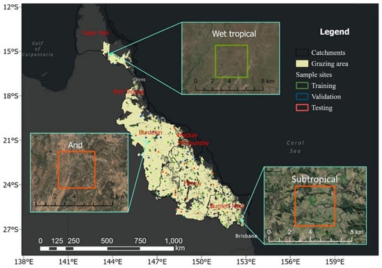
Figure 1.
Spatial distribution of training (green), validation (blue), and testing (red) sample sites. The extent of grazing area on the map corresponds to the grazing native vegetation class from the Queensland Land Use Mapping [57].
2.2. Datasets
In this study, in addition to past ground cover data, climate (e.g., rainfall and temperature) and hydrological (e.g., soil moisture and runoff) data were also used to predict future ground cover. These climate and hydrological factors have been demonstrated to have a substantial impact on land conditions [58,59,60], especially in Australia’s tropical semi-arid rangelands. In Australia, rainfall and temperature, as well as soil moisture and runoff datasets, are available for the entirety of the continent and encompass a lengthy historical period.
2.2.1. Ground Cover Data
This study used the seasonal (three-monthly) ground cover data [20,22,61] as the target, which have been derived from the seasonal fractional cover product [21,62]. The fractional cover product quantifies the proportion of bare ground, green, and non-green cover, but it does not distinguish tree, mid-level woody foliage, and non-woody vegetation. The ground cover product then separates the ‘persistent green’ cover from the total cover to obtain the ‘true’ ground cover estimate [20]. This adjustment of the underlying spectral signature of the fractional cover images resulted in a ground cover estimate, which is primarily the non-woody vegetation. The ground cover product has been proven to be a representative indicator of grazing land conditions in GBRCA [24] and has been used as the input data in the existing land condition management tools [29,30].
Herein, the ground cover is defined as 100–bare ground (Band1), resulting in a scale that ranges from 0 to 100 as a percentage. The representative seasonal ground cover was based on the three-monthly composites of Landsat (Landsat 5 TM, Landsat 7 ETM+, and Landsat 8 OLI) satellite images with masks representing missing data due to persistent cloud in the three-month window. This product, thus, captures variability in ground cover on a seasonal time scale and a 30 m spatial resolution, forming a consistent time series from December 1987 to the date of analysis (August 2023). The dataset was downscaled to [0, 1] by multiplying by 0.01 prior to being fitted into the deep learning models. The ground cover data are accompanied by a mask with ‘1’ representing a data gap, and ‘0’ representing valid data values.
2.2.2. Climate Data
In this project, historical climate data, including rainfall and temperature, were used to analyze and predict the change in ground cover. These climate data were from Scientific Information for Land Owners (SILO) datasets [63] hosted by the Department of Environment and Science (DES), Queensland Government. These data were constructed from observational data obtained by the Australian Bureau of Meteorology (BOM) [64]. The products were delivered as gridded data with 0.05-degree resolution in daily intervals, and in this study, only the seasonal means of rainfall and temperature were used. The resultant dataset was firstly resampled to 30 m and the same projection as the ground cover data and then normalized to [0, 1], following equation 1 to accelerate the convergence speed, reduce training time, and improve the prediction accuracy of the model [65]:
where is the normalized climate data; is the original data; and are the minimum and maximum of the original dataset.
2.2.3. Hydrological Data
The Australian hydrological data from BOM [66] were utilized in this study. These data are based on the Australian Water Resources Assessment Landscape model (AWRA-L [67]), which simulates the water flow through the landscape, as well as the vegetation and soil, before exiting via evapotranspiration, runoff, or deep drainage into the groundwater. Key outputs from the AWRA-L model include surface runoff, soil moisture of different layers, evapotranspiration (potential and actual), and deep drainage. These data are delivered in daily intervals and at a 0.05-degree resolution since 1985. In this study, the daily outputs of AWRA-L were aggregated to seasonal data by calculating the mean values of each season at each pixel. Among the AWRA-L outputs, only soil moisture in the root zone and surface runoff, which have a more direct impact on ground cover, were utilized. Like the climate data, the hydrological data were also resampled to the ground cover projection and normalized to [0, 1].
2.2.4. Data Preparation
Datasets in this study were grouped into three categories: (1) target feature; (2) mask; and (3) auxiliary features. The target feature is the feature to be predicted, i.e., ground cover. It is the first channel of the input image data and the only channel in the output image. The mask feature, serving as the second channel, derives from the ground cover dataset and distinguishes between valid ground cover and data gaps. While it forms the second channel of the input image, it does not appear in the output. The mask feature is important to determine the validity of the ground cover data. The auxiliary features consist of the climate and hydrological data, including rainfall, temperature, soil moisture, and runoff, which are incorporated into the input image but excluded from the output image. These features are important environmental factors that affect ground cover. Auxiliary datasets correspond to channels three to six. The information about the different channels in input image data is summarized in Table 1.

Table 1.
Summary of channels in input images.
For every training, validation, and testing site, all the respective datasets were cropped to the confines of the site, resulting in each channel of the input data having a spatial size of 128 × 128 pixels. The timeframe of this research extends from December 1987 to August 2023, contingent upon the availability of ground cover data. As such, within this timeframe, there are 143 seasonal records for each dataset. In every site, the cropped datasets were then arranged and combined along the channel domain, adhering to the order specified in Table 1. This resulted in a merged dataset with a shape (height × width × channel × seasons) of 128 × 128 × 6 × 143. The merged dataset was then segmented along the temporal (season) domain into data sequences, each encompassing a window length of 16 seasons and advancing by a single-season step. Consequently, each site comprises 128 data sequences, with each sequence conforming to a shape of 128 × 128 × 6 × 16. In total, the number of data sequences for training (50 sites), validation (25 sites), and testing (25 sites) were 6400, 3200, and 3200, respectively.
3. Methods
3.1. Overview of Methodology
As shown in Figure 2, this study compared two distinct spatio-temporal deep learning prediction methodologies and two training scales. The two deep learning-based spatio-temporal prediction methods included the original Convolutional LSTM Network (ConvLSTM [45]) and the more advanced memory-prediction framework named Predictive Recurrent Neural Network (PredRNN [51]).
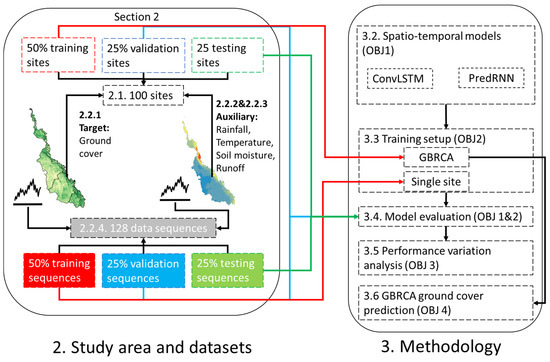
Figure 2.
An overview of the workflow.
The two training scales include GBRCA training and site-specific training. The GBRCA training was based on the ground cover data across all training sites, while the site-specific training was only provided with the first half of the ground cover data for a single site. For both training scales, 50% of the data was used for training, 25% for validation, and 25% for testing. Details about data splitting are shown in Section 3.3.1.
The best method was applied to understand the variation in model performance and predict the ground cover on the GBRCA scale. Section 3.1 and Section 3.2 are aligned with objective 1 and objective 2, whereas Section 3.5 and Section 3.6 outline the methodologies to accomplish objectives 3 and 4, respectively.
3.2. Spatio-Temporal Models
The ConvLSTM model has been used to forecast MNDWI and demonstrated superior performance compared to several baseline approaches such as RNN and Fully connected long short-term memory (FC-LSTM) [49]. However, ConvLSTM, as well as many other follow-up approaches, are deficient in retaining spatial information. Because land condition management relies on the precise demarcation of paddocks, spatial information is of paramount importance, so the PredRNN model, which is optimized to capture spatial details, was included as another model to investigate.
3.2.1. ConvLSTM Model
The ConvLSTM [45] integrates the Long Short-Term Memory model (LSTM) and the Convolutional Neural Network (CNN) to resolve spatiotemporal sequence forecasting problems. The ConvLSTM distills spatial information by exploring convolution operators for both the state-to-state and input-to-state recurrent transitions. In contrast to the standard LSTM, which does not directly model spatial correlation, ConvLSTM can simulate spatial and temporal structures simultaneously. However, in a multi-layer ConvLSTM network, the spatial representations encoded layer-by-layer are not transmitted to the subsequent time step. Thus, the first layer at the current timestep largely ignores the spatial structure that had been memorized by the last layer at the previous step. Furthermore, the ConvLSTM deploys a single memory cell to concurrently handle long-term and short-term dynamics, thereby substantially limiting the model’s overall performance in dealing with complex spatiotemporal variations.
3.2.2. PredRNN Model
To overcome the above challenge of ConvLSTM, the PredRNN model [51] adopted a new zigzag RNN architecture named spatiotemporal memory flow. The zigzag memory flow not only propagates in a bottom–up direction within a timestep but also in a drop-down direction, thus enabling the transfer of the spatial representations to the subsequent time step. This innovative memory flow enhances the state transition of ConvLSTM, thereby reducing the loss of spatial information between successive time steps. PredRNN also introduced a pair of memory cells for the short-term and long-term dynamics, respectively. These twin memory cells function nearly independently, each being explicitly decoupled from the other. Such a double-flow memory transition mechanism can achieve both short-term recurrence depth and long-term coherence. Furthermore, PredRNN has substituted the standard sequence-to-sequence training framework with the method of reverse scheduled sampling. This means instead of using the previous prediction to model the next prediction in the sequence, PredRNN randomly uses either the previous predicted or the previous observed images to predict the next time step, which has been proven efficient for learning jumpy steps in the time series. Nonetheless, in contrast to ConvLSTM, PredRNN, owing to its novel memory flow and the additional memory cell, demands a substantially larger memory and extended training duration.
3.3. Training Setup
3.3.1. Data Split for Different Training Scales
In this study, the data were divided into 50% training, 25% validation, and 25% testing datasets. The training dataset was used to fit the model parameters, while the validation dataset was employed to tune hyperparameters and implement early stopping, ensuring that the model did not overfit the training data. Although the validation dataset was used in the training process, it remained separate from the training dataset and was not used to adjust the model parameters directly. The testing dataset, comprising 25% of the data, was kept completely independent of the training and validation processes and was used solely to evaluate the model’s final performance. Two different data-splitting methods were used for different training scales, respectively.
- GBRCA training: As Figure 1 shows, all data sequences in the training sites were used for training, validation sites for validation, and testing sites for testing. Therefore, there were 6400 data sequences used for training (50 sites × 128 data sequences). In this case, a single trained model was obtained for the entire GBRCA, and the model was applied to all sites in this region;
- Site-specific training: Instead of splitting the training, validation, and testing datasets according to sites, for each individual site, the 128 data sequences along the time series were split into 50% training, 25% validation, and the final 25% testing datasets. The model was specifically trained for the site.
Comparing the two training scales, the site-specific training received substantially less (1/100) data and was more efficient for a single-site application but could not be reused for other sites. In contrast, the GBRCA training was heavy and time-consuming, but once finished, the model could be used to predict future ground cover in any GBRCA site.
3.3.2. Model Structure
Figure 3 shows the structure of the model in this study. Along the temporal dimension, each input data sequence with the shape of 128 × 128 × 6 × 16 was divided into the context sequence (first 8 seasons) and the target sequence (last 8 seasons). The context was defined as the prior sequence that is available for the model to learn the spatiotemporal information, while the target represents the future sequence to be predicted. Input data in both context and target sequence were divided into the ground cover feature, the mask feature, and the auxiliary feature along the channel dimension (details in Section 2.2.4). The output sequence only contains the ground cover feature.
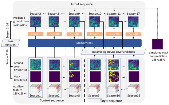
Figure 3.
Overview of the model architecture.
The context sequence was directly fed into the memory cells (i.e., ConvLSTM or PredRNN) to produce the output with a 2D convolutional layer followed by batch normalization. For the target sequence, the input data were not directly fed into memory cells. Instead, they were used in conjunction with the previously predicted ground cover in accordance with the resampling method. This process involved the random sampling of output and input ground cover as well as the mask data, which was then concatenated with the auxiliary data along the channel domain. The resulting synthesized data shared the same dimensions as the input and were subsequently fed into the memory cells. In this step, a simulated mask with zero gap was generated for all the predicted ground covers. Two sampling methods were used in this study. The first method was for standard sequence prediction of recurrent neural networks, which purely used the prediction result from the previous step to predict the next step, and the true previous step in the target sequence is unknown, i.e., non-sampling. This non-sampling method completely hides the information in the target sequence and is used for the original ConvLSTM. Although such a method can simulate the reality that only context image is available, one problem is that mistakes made early in the sequence generation process are fed as input to the model and can be quickly amplified [68]. Therefore, PredRNN [51] adopted the Reverse Scheduled Sampling (RSS) method during training. This method relies on using random predictions as replacements for observations under decreasing probabilities, thereby ensuring that as the training progresses, the model steadily learns more about long-term dynamics [51]. In this study, we adhered strictly to the original workflows of ConvLSTM and PredRNN, so RSS was not applied to ConvLSTM. Although different sampling methods were used in ConvLSTM and PredRNN in the training stage; only the non-sampling method was applied to the testing step to simulate the reality that only a context sequence was available for prediction.
Finally, the input and predicted ground cover, as well as the input mask in overlapping time steps (i.e., season 2~16), were used to calculate losses. Prior to the calculation, both the input and predicted ground cover were multiplied with 1-mask, thereby ensuring that pixels flagged as data gaps in the input were transmuted to 0 and did not contribute to the extra loss. In this study, the Mean Square Error (MSE) was employed as the training loss, while the ensemble of MSE, Huber Loss [69], and the Structural Similarity Index (SSIM [70]) were used as the measures for validation loss. As MSE and Huber Loss indicate superior performance with lesser values, SSIM operates in the opposite way and indicates optimal performance with larger numbers. To ensure consistency while calculating the ensemble loss, 1-SSIM was used to calculate the ensemble loss:
where is the ensemble loss; , and are the MSE, Huber, and SSIM losses, respectively.
3.3.3. Model Configuration
In this study, models were set up with the PyTorch framework. For the two models, we applied the random search approach to determine the best hyperparameters. The search spaces set for the hyperparameters are [1, 3, 5] for the number of hidden layers, [32, 64, 128] for the number of filters in each layer, and [3, 5, 7] for the kernel size. The hyperparameter tuning was performed on the training and validation datasets for a single site. The performance of both models did not show substantial improvement when the number of layers, the number of filters, and the kernel size exceeded 3, 64, and 5, respectively. As a result, to balance the model accuracy and the training efficiency of the GBRCA-scale model, for both ConvLSTM and PredRNN, 3 layers of memory cells were stacked, with each layer having 64 hidden channels per batch. The size of the convolving kernel was set to 3.
For the training procedure, the batch size for training, testing, and validation was set to 4. The AdamW [71] optimizer was used; the learning rate was set to 0.0001, and the training was set to run for 500 epochs, with early stopping initiated if the validation loss did not improve over 100 epochs for ConvLSTM and 10 epochs for PredRNN. The model was checked after each epoch and saved at the checkpoint with the best validation loss. The optimized model was used for evaluation and application.
3.4. Model Evaluation
Corresponding to our objective (2), in the evaluation stage, for data in training, testing, and validation datasets, the first 8 seasons were used as the context and fed into memory cells to forecast the ground cover in future seasons. The last 8 seasons were used as targets for comparison against the model’s predictions. As the non-sampling method was applied during this evaluation stage, data from the target sequence were not used to predict the following time step.
Firstly, we focused on prediction step 1 in the target sequence (i.e., season 9 in Figure 3) when the memory cell only received observation data in the context sequence. The model performance was evaluated for the entire time series in each site. In this experiment, by iterating all data records in training, validation, and testing datasets, the spatial mean of the target and predicted ground cover for prediction step 1 were calculated and compared to demonstrate the ability of the model to reproduce the next-season ground cover trend in a site. Mean Absolute Error (MAE) and SSIM were also calculated for each pair of targets, and ground cover images were predicted to quantify the temporal variance of the model’s performance.
In addition to the MAE and SSIM for prediction step 1, the changing rates of these two metrics were also evaluated across the sequence from prediction step 1 (season 9) to step 8 (season 16) in the target sequence (Figure 3), noting how the number of predicted results impacted subsequence predictions. For each of the 128 input data sequences in each site, the slope of MAE and SSIM changing from step 1 to step 8 was calculated and defined as the decay rate.
Finally, the model performance was evaluated spatially by comparing the target images to their corresponding predictions. This evaluation was implemented for the data sequence with the lowest ground cover at prediction step 1 (season 9) in the time series, which indicated the worst land condition for a grazing site. For this single data sequence (8 context seasons + 8 target seasons), all the predictions and observations in the target sequence were pairwise visualized and compared to demonstrate the differences between prediction and observation. The absolute differences between the corresponding pair of pixel values were calculated and plotted to highlight the spatial distribution of errors. The histograms of pixel values for target and prediction images were also calculated and compared.
3.5. Performance Variation Analysis
In this study, the performance variation analysis aims to understand the factors that lead to prediction inaccuracy and focuses on the first prediction step. For each testing site, the MAE and SSIM at prediction step 1 were first spatially averaged and then temporally grouped and averaged into four seasons. Next, for each season and site, the mean and standard deviation of the aggregated MAE and SSIM were calculated to illustrate the seasonal and spatial variations in the scoring metrics.
After checking the seasonal and spatial variations, the MAE and SSIM were further averaged across seasons for each site. The correlation between the aggregated metrics and the spatio-temporally averaged ground cover, spatial standard deviation of ground cover, rainfall, temperature, soil moisture, and runoff were calculated in the 50 validation and testing sites to indicate the impact of these environmental factors on scoring metrics.
3.6. GBRCA Ground Cover Prediction
In this study, we used the GBRCA model with superior accuracy to predict the ground cover in the entire GBRCA grazing area with 300 m resolution, which is sufficient for catchment-scale management. Firstly, the target area was divided into grids with the size of 38,400 × 38,400 m2 (1280 × 1280 30 m Landsat pixels) and 50% overlapping both horizontally and vertically. Then, the target, mask, and auxiliary data in the last 16 seasons from September 2019 to August 2023 were extracted in each grid and resampled down to 128 pixels × 128 pixels × 16 seasons, so the pixel size increased from 30 m to 300 m. Next, the resampled dataset was used as the input dataset to the trained model with all 16 seasons as context, so the last predicted frame was the prediction for the ground cover in the season of September 2023~January 2024. Finally, the prediction for each grid was mosaiced as a single image for the GBRCA.
4. Results
4.1. Model Evaluation
4.1.1. Single-Site Evaluation
Although the PredRNN model was evaluated across all validation and testing sites, this section presents only the detailed results for one arid testing site (zoomed-in arid site in Figure 1). This is also the site where site-specific models were trained. This site in the Burdekin catchment is among the barest sampled sites with low ground cover. It is imperative to understand the accuracy of the model for such sites. When comparing the first step prediction of ground cover to the target (Figure 4), the time series of spatially averaged prediction matched the observation very well with MAE < 5% for the majority of the dates, despite the seasonal and longer-term variations. The troughs of prediction (dashed line) are mostly lower than the observation (solid), while the peaks follow the opposite trends, showing the under and over-estimation of ground cover in dry and wet seasons, respectively. Although cloud cover (grey bars) was higher during wet seasons with increased ground cover, the model’s accuracy was not significantly affected by this increase. To quantify the model performance, the MAE and SSIM were calculated for each pair of prediction and observation. The MAE fluctuated around 3% with a temporal average of 3.3% and a maximum of up to 8%. The average decay rate was 0.340%/step. There was a negative correlation between the MAE and its decay rate, so a smaller MAE and better model performance at step 1 decayed quicker. The SSIM on this site was generally above 0.6, with the best score reaching about 1. The average decay rate was about −0.035/step. Unlike MAE, larger SSIM, which represented better model performance, had medium or small magnitude.
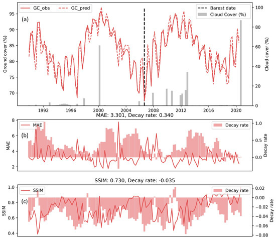
Figure 4.
Time series of ground cover prediction (a) and scoring metrics (b,c) for PredRNN. In plot (a), the solid and dash lines are the predicted and target ground cover at prediction step 1, respectively. The grey bars are the cloud cover rate, and the black vertical line indicates the date with smallest ground cover. The solid line in the plot (b,c) shows the spatial average of MAE and SSIM at prediction step 1, respectively, and the bars are the corresponding decay rate from prediction step 1 to step 8 (season 9~16 in target sequence in Figure 3).
To better understand the spatial distribution of errors and the decay of model performance, for the data sequence with the lowest ground cover (based on the prediction step 1), the images from the prediction to the target were compared (Figure 5). This data sequence spans from September 2004 to June 2008 (with the first prediction season in September 2006). The temporal location of this data sequence is indicated in Figure 4. Given the eight context images in the first row of Figure 5, the PredRNN model was applied to predict the subsequent eight images in the second row, and the results are presented in the third row. For the first prediction step (first column), the PredRNN model reproduced the target season 1 very well, not only visually but also quantitatively. The difference in the third row was generally less than 3%, and the histograms of the target and prediction in the fourth row were very similar. From the second to the fifth prediction steps, the model’s performance did not decay substantially. Starting from the sixth prediction step, the offset of the prediction became prominent and continued to increase. Despite the decay of performance, the PredRNN model was still able to capture the general trend of seasonal variation even for the last prediction step. In summary, both spatial and temporal evaluation demonstrated the high accuracy of the PredRNN model in predicting ground cover in such hotspots of poor land conditions.
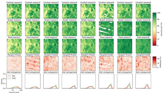
Figure 5.
Comparison of predicted and target ground cover maps for different prediction steps of the data sequence highlighted in Figure 4. The first row shows the context images used to generate predictions. The second and third rows show the target images and their predictions. The fourth row shows the absolute difference between the targets and predictions, while the last row shows the histogram comparison of observations (targets) and predictions.
4.1.2. Scoring Metrics for All Sites
Instead of showing detailed evaluation metrics for all training, validation, and testing sites as in Section 4.1, the scoring metrics for all 100 sample sites were aggregated and summarized. The training sites had the best scoring metrics, and the testing sites had the worst scores in terms of the largest median MAE (Figure 6a) and the smallest SSIM (Figure 6b). However, the difference among the training, validation, and testing datasets was not substantial. For each group of sites, the scoring metrics varied substantially. Both the largest MAE and the smallest SSIM appeared in the training instead of the testing sites. Regarding the decay rates, especially for MAE, the difference among training, validation, and testing became more prominent. The median MAE decay rate was only 0.14%/step for the training dataset but increased to 0.21%/step for the validation and 0.16%/step for the testing datasets.
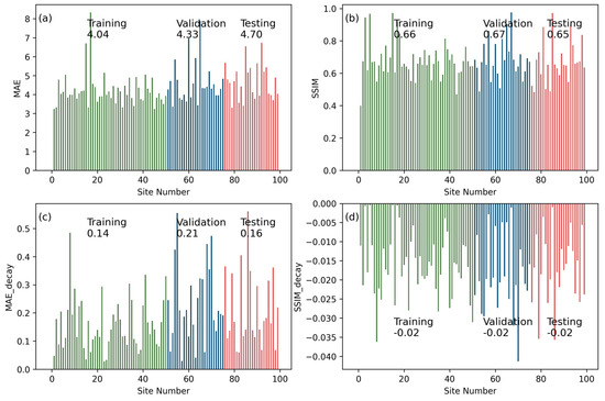
Figure 6.
Statistics of scoring metrics of PredRNN model for training, validation, and testing sites. Plot (a), (b), (c), and (d) are the results for MAE, SSIM, MAE decay, and SSIM decay, respectively. The MAE and SSIM results are the spatial–temporal mean for the first prediction step. Numbers above/below the bars are the median values of the metrics among all 100 sites.
4.2. Model Performance Comparison
4.2.1. Comparison of Different Models
In this study, the performance of ConvLSTM and PredRNN in the validation and testing sites was compared (Table 2). Among the two models, PredRNN had smaller MAE and larger SSIM values on average (for the prediction step 1), demonstrating its superior ability to predict the next season’s ground cover. However, compared to ConvLSTM, PredRNN exhibited a larger magnitude of decay rate for MAE and SSIM from prediction steps 1 to 8. This indicates that the advantage of PredRNN becomes less prominent when predicting longer-term (e.g., multiple seasonal) ground cover change.
Table 2.
Performance comparison between PredRNN and ConvLSTM. The scoring metrics in the table are the average of the 50 validation and testing sites.
4.2.2. Comparison of Different Training Scales
This study also trained the two models site-specifically and compared different training scales for an example site (i.e., arid site in Figure 1). The comparison was initially implemented for all the data sequences with aggregated scoring metrics (Figure 7). For the first prediction step, all the models and training scales were able to reproduce the spatial mean of ground cover to a great extent, with the PredRNN model trained on GBRCA (PredRNN_GBRCA) providing the best matching (a1), especially in dry seasons. Regarding MAE and SSIM for the prediction step 1 (b1 and c1), PredRNN_GBRCA had the smallest MAE and the largest SSIM values for almost every data record, which was also proved by the box plots (b2 and c2), where PredRNN_GBRCA had the smallest MAE and the largest SSIM for every percentile. Therefore, PredRNN_GBRCA is superior in predicting the next season’s ground cover. The PredRNN trained on the individual site (PredRNN_site) had the second-best MAE value (b2), which was even better than the ConvLSTM_GBRCA, showing the potential of PredRNN to be trained and used site specifically. For SSIM, the advantage of PredRNN_site was not apparent compared to ConvLSTM_site (c2), and the latter model had better performance in dry seasons (c1). Despite its superiority in the prediction step 1, PredRNN_GBRCA had the highest increasing rate for MAE (d1 and d2) and decreasing rate for SSIM (e1 and e2). ConvLSTM_site and ConvLSTM_GBRCA outperformed in decay rates in this site, so the advantage of PredRNN is undermined when predicting longer-term trends.
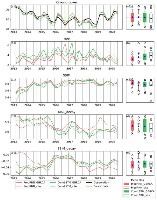
Figure 7.
Comparison of different models and training scales for the arid testing site (site 78) in Figure 1. Plots in the first column (a1–e1) shows the temporal variation of accuracy. Ground cover, MAE, and SSIM are based on the prediction step 1. ConvLSTM_site and PredRNN_site (dash lines) are model-trained sites, specifically. ConvLSTM_GBRCA and PredRNN_GBRCA (solid lines) are models trained on the GBRCA scale. The brown vertical line indicates the date with the least ground cover. The boxplot in the second column (a2–e2) summarizes the statistics of the time series in the first column. The blue triangle is the mean. Boxes extend from 25th to 75th percentiles, and whiskers from 5th to 95th percentiles. Circles represent outliers.
After comparing the aggregated performance of different models and training strategies, the image comparison was performed to visualize the spatial details for the indicated data sequence (dashed grey line in Figure 7), which had the barest prediction step 1. For the prediction step 1 (first column in Figure 8), all the models and training strategies predicted the observation reasonably well visually; however, quantitively, PredRNN_GBRCA has the most similar histogram to the observation, followed by ConvLSTM_GBRCA. The site-specific training methods underperformed in this prediction step. From prediction step 2 (second column) to prediction step 8 (eighth column), although the performance of PredRNN_GBRCA decayed substantially, it was still one of the best methods. PredRNN_site was the other method that had competitive performance in these prediction steps. In comparison, the ConvLSTM based methods had worse performance.
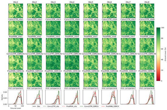
Figure 8.
Comparison of different models and training strategies for target images in a single data sequence indicated in Figure 7. First row shows results from observation. Second to fifth rows are prediction results from different trained models. The last row shows comparison of histograms.
4.3. Model Performance Variation Analysis
This study evaluated the seasonal variation in the PredRNN performance (Table 3). Ground cover in GBRCA is at its peak in the southern hemisphere’s autumn and winter and reaches the lowest point in spring (September to November). Meanwhile, the Reef Protection Regulations [25] set by the Queensland Government in Australia require that ground cover in GBRCA be assessed at the end of September. Therefore, spring (September to November) is the season that demands the greatest model accuracy. For both MAE and SSIM, the seasonal variation in performance is substantial. For seasons with larger ground cover (e.g., winter from July to August), the MAE was minimal, but the SSIM is the second worst. On the other hand, December to February (summer) has the worst MAE but the best SSIM. As the key season to focus on, spring has the second-worst MAE but the second-best SSIM.
Table 3.
Seasonal variation in MAE and SSIM for the PredRNN model. Values in this table are the average across all validation and testing sites.
In addition to the seasonal variation, the spatial distribution of these scoring metrics (Figure 9) was explored to understand the relationship between model performance and the geographical location of sample sites. Most of the extremely large MAE values (large scatter points) were in wet tropical and coastal regions, while the MAE for sites in inland arid areas (e.g., landward sites in the Burdekin catchment) were smaller and more stable. On the other hand, most of the above sites (except those in Wet Tropics) with large MAE values also had large SSIM values, which indicates better structural similarity. The reason for this contradictory result is that grazing areas in coastal regions are relatively small compared to the Burdekin. The sample sites in coastal regions are more likely to cover not only grazing but also other land types and, thus, have more complicated and diverse land covers, which would benefit the SSIM but undermine the MAE values. For sites in Wet Tropics, the extremely high cloud cover rate resulted in large data gaps even with seasonal composites, which, thus, undermined model performance in terms of both MAE and SSIM.
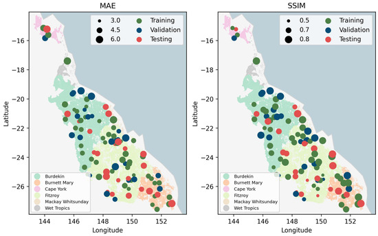
Figure 9.
Spatial distribution of MAE and SSIM. The two metrics are aggregated as the spatio-temporal mean for the first prediction step. The smoke-white and light-blue backgrounds represent land and sea, respectively. Polygons with different colors are the grazing areas in different catchments. The varying sizes of scatter points indicate the magnitude of scoring metrics.
To further analyze the reason behind the performance variation, the site-aggregated MAE and SSIM were correlated to other environmental factors (Figure 10). Firstly, the spatio-temporal mean of ground cover GC_mean has a strong correlation with rainfall (), runoff (), and soil moisture (). The spatio-temporal standard deviation GC_STD has a strong correlation with temperature. These results demonstrate the necessity of incorporating climate and hydrological variables. Regarding the sensitivity of model performance to different factors, for MAE, it was negatively correlated () to ground cover, showing that the PredRNN could perform better for sites with large (GC_Mean). The MAE was also positively correlated () to GC_STD, indicating that the performance was poorer for sites with large spatial variation in ground cover (more diverse land cover). Among climate and hydrological factors, the correlation of MAE to rainfall and temperature () was relatively weak, while runoff and soil moisture had a larger impact on the MAE with a positive correlation coefficient above 0.4, showing that the MAE was larger in sites with large rainfall, runoff, and soil moisture. SSIM was more sensitive and positively correlated to most of the listed environmental factors except temperature. Sites with large average and spatial variation in ground cover, more rainfall and runoff, as well as large soil moisture had better SSIM in general. In addition to the correlation between scoring metrics and different environmental factors, Figure 10 also demonstrates the substantial negative correlation between GC_Mean and GC_STD (). The main reason is that most sites with large ground cover (GC_Mean) are in NRM regions (e.g., Wet Tropics and Mackay Whitsundays) with small grazing areas, so these sites are more likely to cover multiple land uses and result in large spatial variation in ground cover (GC_STD).
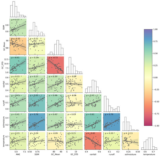
Figure 10.
Correlation of scoring metrics to different environmental factors. GC_mean and GC_STD are the spatial–temporal mean and standard deviation of ground cover for a site. The solid line in each pair plot is the linear fit for the scatter points. ρ is the Pearson correlation coefficient. The background color gradient indicates the magnitude of ρ.
4.4. GBRCA Next-Season Ground Cover Prediction
In this study, the ground cover change for the entire GBRCA grazing area in the last dry season (from September 2022~November 2022 to December 2022~February 2023, Figure 11) was predicted and compared with the observations. The comparison between the observation (Figure 11a,b) and the prediction (d and e) for the last season in the context sequence (June 2022~August 2022) and the first season in the target sequence (September 2022~November 2022) demonstrated the ability of the PredRNN model to reproduce historically and predict future ground cover on a large spatial scale even with a different resolution (300 m) to the training (30 m). Next, the change in ground cover (c and f) from the wet to the dry season was compared. Both observations and predictions showed that the ground cover for almost the entire GBRCA decreased, and the magnitude of the decrease was up to 20%. The hotspots of decreased ground cover appeared in the inland part of the Burdekin catchment, but the magnitude of a decrease in these regions was overestimated by the PredRNN model. The overestimation was also evidenced in the inset histograms in (c) and (d). Compared to observations, histograms for prediction clearly had more shifting toward the low ground cover from the wet to the dry season.
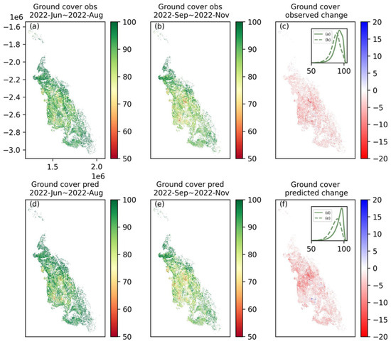
Figure 11.
Ground cover for grazing areas in the GBRCA. (a,d) are the ground cover maps for June 2022 to August 2022 (the last season in the context sequence) from observation and prediction, respectively; (b,e) are the results for September 2022 to December 2022 (the first season in the target sequence); and (c,f) are the maps for the change in ground cover in the above two seasons. The inset plots in (c,f) compare the histograms of pixels in the two seasons.
The statistics of the comparison between observations and predictions from September 2019 to September 2023 are summarized in Figure 12. Regarding the spatial average, although the prediction described the temporal trend of observation, the ground cover was generally overestimated, and the offset between observation and prediction was up to 5%. The MAE varied from 2 to 5 percent, and the standard deviation of the absolute error in the spatial domain ranged from 0 to approximately 10%. The SSIM for all pairs of observation and prediction was above 0.79, and the best value was 0.81. More importantly, the increment of ground cover predicted by the observation was very similar to the observation in dry seasons (e.g., September 2019, 2020, 2021, and 2022). This finding demonstrates the superior applicability of the PredRNN model in predicting the decrease in ground cover in dry seasons, which is the most important trend for managing grazing land.
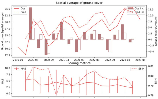
Figure 12.
Accuracy of GBRCA ground cover prediction from September 2019 to September 2023. The solid and dashed lines in the first plot are the spatial average of observation and PredRNN prediction. The filled and unfilled bars represent the increment (negative value for decrement) of observation and prediction, respectively. In the second plot, the solid line with error bars represents the MAE and the standard deviation of the absolute error, while the dashed line represents the SSIM.
5. Discussion
5.1. Scalability
There are two main factors affecting the scalability of the proposed method to larger spatial scales. The first factor is the impact of the spatial density of training sites on the model accuracy, and the other one is the time and resources required for training. These two factors are discussed in Section 5.1.1 and Section 5.1.2, respectively.
5.1.1. Impact of the Spatial Density of Training Sites
In this study, the PredRNN model was trained on 50 sampling sites distributed across the entire GBRCA and covered diverse environments with 28 sampling sites in the Burdekin catchment. However, such large coverage also means a smaller number of training sites for each type of environment. To investigate the impact of the training scale and evaluate the scalability of the PredRNN model, another model was trained on 50 sampling sites that are all located in the Burdekin catchment, which has the largest grazing area. Therefore, there are more training sites representing the grazing area within the same catchment.
The predicted ground cover for the dry season (September to December 2022) by the two models trained on different scales were then compared (Figure 13). Qualitatively, models trained for both the Burdekin catchment and the GBRCA reproduced the spatial variation in ground cover (b and c). When focusing on arid pixels with relatively low ground cover (yellow and red areas) in observation (a), the ground cover for most of these pixels was clearly overestimated by the Burdekin prediction (b) while underestimated by the GBRCA prediction. These can be visualized by the blue area (overestimation) in (d) and the red area (underestimation) in (e). Quantitatively, these two models showed underestimation and overestimation ranging from −10% to 10% (Figure 13d,e). The model trained on the GBRCA with a larger scale had a slightly larger MAE than the model trained specifically on the Burdekin catchment, but the histogram from the former approach more closely matched the observation. Therefore, despite being trained with more localized ground cover data, the Burdekin prediction does not improve the model performance substantially, especially in predicting low ground cover regions, which are the focus of land condition management. This result demonstrates that the spatial scale for the sampling of training sites has a limited impact on the model accuracy. Sampling the training sites less densely over larger spatial scales does not significantly undermine the model performance. However, as the Burdekin catchment also covers diverse environments, it is not representative of the sampling of training sites with uniform and consistent land covers. Further analysis can be conducted in the future to investigate the impact of the consistency of training sites on the model accuracy.
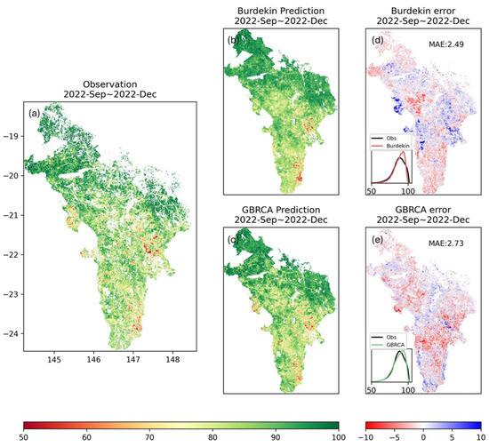
Figure 13.
Comparison of PredRNN model trained on sites in GBRCA and Burdekin. The first column (a) is the observation for the season from September to December 2022; the second column (b,c) shows predictions for the same season by different trained models. The last column (d,e) shows the errors (i.e., prediction–observation) of the different predictions. Inset plots in the last column compare the histograms for observation and model prediction.
5.1.2. Time and Resources
Although the PredRNN model performance is insensitive to the density of training sites, having sufficient training data to cover different environments remains important. The time and resources required for training increase significantly as more training data is used. For the models trained using 50 training sites and 6400 data sequences (128 × 128 × 6 × 16), the time and resources required are summarized in Table 4. The ConvLSTM and PredRNN models were trained on NVIDIA V100 GPUs with 16 GB and 32 GB memory, respectively. ConvLSTM took 137 h and 210 epochs to achieve the best validation score. In comparison, PredRNN required only nine epochs to reach its best state. Although the training time required by PredRNN for each epoch is about seven times larger, the PredRNN model was more efficient in training for its fast convergence. This suggests that the PredRNN model is not only more accurate but also potentially more efficient to train. However, it is worth noting that this conclusion is based on differences in GPU memory. The PredRNN model required substantially more memory than the ConvLSTM model. When computational power is limited, ConvLSTM becomes a more practical solution for large-scale training.
Table 4.
Time and resources required to train different spatio-temporal prediction models at GBRCA scale.
5.2. Implications
This study explored the applicability of deep learning-based spatio-temporal prediction models to predict future ground cover on different spatial scales with varying quantities of training data. The results from this study demonstrate that both the relatively simple model ConvLSTM and the more complicated model PredRNN predicted the next season’s ground cover with high accuracy given the past ground cover, as well as climate and hydrological conditions for sample sites across the GBRCA for training. The trained models can be efficiently applied to any given grazing area to produce high-resolution (i.e., 30 m) and high-accuracy (i.e., MAE < 5%) ground cover maps one season earlier than products derived from the actual satellite images. The existing early-alert tool, pasture growth alert, used in the GBRCA [28], is based on empirical linear and curvilinear relationships between land conditions and rainfall. The over-simplicity of this tool undermines its robustness for land condition management. Additionally, the pasture growth alert, along with many other land condition prediction methods [22] in the GBRCA, aggregates spatial information and ignores variations in land conditions within the area of interest. Mapping-based methods have also been applied in the GBRCA to identify potentially degraded lands by analyzing historical trends in ground cover [30,72]. However, these methods did not predict the ground cover change directly. Given the limitations of existing tools, the high accuracy and high resolution of deep learning methods offer novel opportunities for land condition management in the GBRCA. Firstly, the high accuracy of the new tool will enhance the confidence of grazing property owners and local environmental authorities to take proactive approaches to avoid land degradation. Secondly, the high spatial resolution of the map for future ground cover facilitates the prioritization of land condition management within each paddock more precisely. Thirdly, the new approach enables the mapping of future ground cover for the entire GBRCA at coarser scales (i.e., 300 m). This large-scale map can be applied to analyze the common and unique characteristics of regional ground cover change, which may help local authorities adopt land condition management plans in response to extreme climate events such as drought.
While ConvLSTM and other spatio-temporal deep learning methods have been used to predict LUCC in previous studies, their applications have been limited to single sites with study areas smaller than 5000 km2 [48,49,73,74]. To extend this approach to the GBRCA, which spans over 300,000 km2, we innovatively trained the model on data sampled from various sites across the entire region. The success of this study demonstrates the applicability of deep learning models for spatio-temporal predictions not only at individual sites but also across large, diverse landscapes. The comparison of different models and training scales used in this study can be applied to inform the model selection in the future. Comparing ConvLSTM to PredRNN, the relatively complicated structure of the latter model gave it better accuracy in terms of MAE and SSIM, especially for the first prediction step. However, the superior accuracy of PredRNN quickly decayed when predicting longer-term ground cover. Although the complicated structure of PredRNN required a longer time to finish the training of one epoch, the faster convergence of the model allowed it to obtain the optimum parameters in substantially fewer epochs. As a result, the training of PredRNN was more efficient overall. However, the implementation of PredRNN on GBRCA required a larger amount of GPU memory than ConvLSTM, and the latter model is still the better option when the computational capability is limited.
5.3. Limitations and Future Directions
Although the PredRNN model works relatively well for forecasting the next season’s ground cover, it is less robust when predicting seasons beyond that. The decay of performance limits the model’s application to the short term (e.g., <1 year). When applying this model for longer-term forecasting, the spatio-temporal information is lost gradually. To overcome this limitation, it is worth exploring more advanced models that are superior in predicting long-term trends.
The availability of auxiliary datasets is another factor that prohibits the model application to seasons beyond the next season. All the auxiliary datasets used in this study were from historical measurements or hindcasts. Since these datasets are imperative, the model cannot perform well without them. Short-term (e.g., weeks) forecasts for rainfall and temperature are available from BOM, but forecasts for the next season are limited. The soil moisture and runoff data were obtained from a numerical model, so forecasts are achievable, but existing datasets only cover the historical range. To avoid the limitations related to auxiliary datasets, future research can also incorporate the auxiliary features as targets to predict and integrate the forecasted auxiliary data for future predictions. It is also worth evaluating the importance of the auxiliary datasets to the model accuracy and exploring the applicability of models simply based on the past ground cover.
Even when predicting for the next season, uncertainties remain. The most important one to note is the seasonal and regional variation in the model performance. As the Australian spring (September to November) is the most important season to predict, the model scoring metrics are not the best (the second best in SSIM and the second worst in MAE) this season. Despite the bias, this model was precise at predicting the relative ground cover change from a wet to a dry season. Additionally, the model performance is impacted by other environmental factors. Sites with poor ground cover were not predicted as well as those with large ground cover while the former category is usually more at-risk. For the entire GBRCA, the ground cover was overestimated in wet regions but underestimated in dry regions. The potential reason for the larger MAE in dry seasons (i.e., spring and summer) and poor ground cover conditions is the bias of training data toward wet seasons and high ground cover. A large portion of sample sites is located in wet tropics where seasonal variations in land conditions are negligible, and ground cover remains consistently high, similar to wet seasons. Therefore, although the ground cover data are almost evenly distributed across all seasons, more data are representative of wet seasons and high ground cover than dry seasons and poor ground cover. As a result, the models were fitted to have better accuracy for wet seasons and high ground cover, while the ground cover in arid seasons and sites was mostly underestimated, which can result in more protective land condition management practices. As a potential solution to improve the model performance for dry season and poor land conditions, more sites can be sampled in arid regions to balance the low and high ground covers in training.
6. Conclusions
In this study, we applied spatio-temporal deep learning models, including ConvLSTM and PredRNN, for ground cover prediction in the GBRCA. These models, especially PredRNN, showed promising accuracy for the next-season prediction with an average testing MAE of about 4% and SSIM of about 0.65%. The model accuracy has considerable seasonal and regional variations with lower values in arid regions and during dry seasons, likely due to an imbalance in the training data.
This study achieved GBRCA-scale (over 300,000 km2) ground cover prediction by training the model on sites sampled across the area of interest. The success of this approach illustrates the potential of spatio-temporal deep learning models for large-scale applications. The results also suggest that while PredRNN offers superior accuracy, it is computationally intensive, whereas ConvLSTM provides a more efficient alternative for scenarios with limited computational resources.
The deep learning models performed well in predicting the next-season ground cover; the decay in model performance and the lack of projections for auxiliary datasets prevent their application to multi-season predictions. If the auxiliary datasets could be accurately predicted in the future, the capabilities for ground cover prediction are likely to expand.
This study’s findings have significant implications for land condition management in the GBRCA. The ability to predict ground cover one season ahead allows for proactive interventions, reducing the risk of land degradation. The high spatial resolution of the predictions enables targeted management practices at the paddock level. Moreover, the scalability of the models to larger areas provides a strategic advantage in regional planning, particularly in response to extreme climate events such as drought.
Author Contributions
Y.M., M.S.J.W. and R.D.R.T. conceived the initial conceptualization; Y.M. performed the analysis and wrote the manuscript draft with the support of M.S.J.W. and R.D.R.T. All authors contributed to the revisions of this manuscript on their specific expertise. All authors have read and agreed to the published version of the manuscript.
Funding
This research was supported by the Reef Catchment Science Partnership jointly funded by the University of Queensland (UQ) and the Department of Environment and Science (DES), Queensland Government.
Data Availability Statement
The code used in this research is available at https://github.com/yongjingmao/ground_cover_convlstm (accessed on 27 August 2024). All the data used in this research is available on request.
Acknowledgments
The authors would like to acknowledge the Remote Sensing Sciences of DES for providing the ground cover and climate data and the Bureau of Meteorology, Australian government, for providing the hydrological data. The authors would also like to offer their sincere gratitude to Dan Tindall, Deanna Vandenberg, Al Healy, Rebecca Trevithick, Rebecca Farrell, and Fiona Watson in DES for providing valuable advice in the preparation of this paper.
Conflicts of Interest
The authors declare no conflicts of interest. The sponsors had no role in the design, execution, interpretation, or writing of this study.
References
- Food and Agriculture Organization of the United Nations. FAOSTAT—Land Use. 2021. Available online: http://www.fao.org/faostat/en/#data/RL (accessed on 27 August 2024).
- ABARES. Land Use of Australia 2010–11 to 2015–16, 250 m; ABARES: Canberra, Australia, 2022. [CrossRef]
- State of Queensland. Reef 2050 Water Quality Improvement Plan 2017–2022. 2018. Available online: https://www.reefplan.qld.gov.au/__data/assets/pdf_file/0017/46115/reef-2050-water-quality-improvement-plan-2017-22.pdf (accessed on 27 August 2024).
- Trimble, S.W.; Mendel, A.C. The cow as a geomorphic agent—A critical review. Geomorphology 1995, 13, 233–253. [Google Scholar] [CrossRef]
- Bartley, R.; Hawdon, A.; Post, D.A.; Roth, C.H. A sediment budget for a grazed semi-arid catchment in the Burdekin basin, Australia. Geomorphology 2007, 87, 302–321. [Google Scholar] [CrossRef]
- Risk, M.J. Assessing the effects of sediments and nutrients on coral reefs. Curr. Opin. Environ. Sustain. 2014, 7, 108–117. [Google Scholar] [CrossRef]
- Baird, M.E.; Mongin, M.; Skerratt, J.; Margvelashvili, N.; Tickell, S.; Steven, A.D.L.; Robillot, C.; Ellis, R.; Waters, D.; Kaniewska, P.; et al. Impact of catchment-derived nutrients and sediments on marine water quality on the Great Barrier Reef: An application of the eReefs marine modelling system. Mar. Pollut. Bull. 2021, 167, 112297. [Google Scholar] [CrossRef]
- McCulloch, M.; Fallon, S.; Wyndham, T.; Hendy, E.; Lough, J.; Barnes, D. Coral record of increased sediment flux to the inner Great Barrier Reef since European settlement. Nature 2003, 421, 727–730. [Google Scholar] [CrossRef] [PubMed]
- Fabricius, K.E. Effects of terrestrial runoff on the ecology of corals and coral reefs: Review and synthesis. Mar. Pollut. Bull. 2005, 50, 125–146. [Google Scholar] [CrossRef]
- Waterhouse, J.; Brodie, J.; Lewis, S.; Mitchell, A. Quantifying the sources of pollutants in the Great Barrier Reef catchments and the relative risk to reef ecosystems. Mar. Pollut. Bull. 2012, 65, 394–406. [Google Scholar] [CrossRef]
- McCloskey, G.L.; Baheerathan, R.; Dougall, C.; Ellis, R.; Bennett, F.R.; Waters, D.; Darr, S.; Fentie, B.; Hateley, L.R.; Askildsen, M. Modelled estimates of fine sediment and particulate nutrients delivered from the Great Barrier Reef catchments. Mar. Pollut. Bull. 2021, 165, 112163. [Google Scholar] [CrossRef]
- O’Mahoney, J.; Simes, R.; Redhill, D.; Heaton, K.; Atkinson, C.; Hayward, E.; Nguyen, M. At What Price? The Economic, Social and Icon Value of the Great Barrier Reef; Deloitte Access Economics: Sydney, Australia, 2017. [Google Scholar]
- Kroon, F.J.; Thorburn, P.; Schaffelke, B.; Whitten, S. Towards protecting the Great Barrier Reef from land-based pollution. Glob. Chang. Biol. 2016, 22, 1985–2002. [Google Scholar] [CrossRef]
- Coggan, A.; Thorburn, P.; Fielke, S.; Hay, R.; Smart, J.C. Motivators and barriers to adoption of Improved Land Management Practices. A focus on practice change for water quality improvement in Great Barrier Reef catchments. Mar. Pollut. Bull. 2021, 170, 112628. [Google Scholar] [CrossRef]
- Australian and Queensland Government. Grazing Water Quality Risk Framework 2017–2022; Australian and Queensland Government: Brisbane, Australia, 2020.
- Pickup, G. New land degradation survey techniques for arid Australia—Problems and prospects. Rangel. J. 1989, 11, 74–82. [Google Scholar] [CrossRef]
- O’Neill, A.L. Satellite-derived vegetation indices applied to semi-arid shrublands in Australia. Aust. Geogr. 1996, 27, 185–199. [Google Scholar] [CrossRef]
- Wallace, J.; Behn, G.; Furby, S. Vegetation condition assessment and monitoring from sequences of satellite imagery. Ecol. Manag. Restor. 2006, 7, S31–S36. [Google Scholar] [CrossRef]
- Jafari, R.; Lewis, M.M.; Ostendorf, B. Evaluation of vegetation indices for assessing vegetation cover in southern arid lands in South Australia. Rangel. J. 2007, 29, 39–49. [Google Scholar] [CrossRef]
- Trevithick, R.; Scarth, P.; Tindall, D.; Denham, R.; Flood, N. Cover under Trees: RP64G Synthesis Report; Department of Science Information Technology, Innovation and the Arts: Brisbane, Australia, 2014. [Google Scholar]
- Scarth, P.; Röder, A.; Schmidt, M.; Denham, R. Tracking grazing pressure and climate interaction-the role of Landsat fractional cover in time series analysis. In Proceedings of the 15th Australasian Remote Sensing and Photogrammetry Conference, Alice Springs, Australia, 13–17 September 2010. [Google Scholar]
- Barnetson, J.; Phinn, S.; Scarth, P.; Denham, R. Assessing Landsat Fractional Ground-Cover Time Series across Australia’s Arid Rangelands: Separating Grazing Impacts from Climate Variability. ISPRS—Int. Arch. Photogramm. Remote Sens. Spat. Inf. Sci. 2017, XLII-3/W2, 15–26. [Google Scholar] [CrossRef]
- Guerschman, J.P.; Hill, M.J.; Renzullo, L.J.; Barrett, D.J.; Marks, A.S.; Botha, E.J. Estimating fractional cover of photosynthetic vegetation, non-photosynthetic vegetation and bare soil in the Australian tropical savanna region upscaling the EO-1 Hyperion and MODIS sensors. Remote Sens. Environ. 2009, 113, 928–945. [Google Scholar] [CrossRef]
- Beutel, T.S.; Shepherd, R.; Karfs, R.A.; Abbott, B.N.; Eyre, T.; Hall, T.J.; Barbi, E. Is ground cover a useful indicator of grazing land condition? Rangel. J. 2021, 43, 55–64. [Google Scholar] [CrossRef]
- Queensland Government. Reef Protection Regulations. 2022. Available online: https://www.qld.gov.au/environment/agriculture/sustainable-farming/reef/reef-regulations/about (accessed on 27 August 2024).
- Navin, M.S.; Agilandeeswari, L. Multispectral and hyperspectral images based land use/land cover change prediction analysis: An extensive review. Multimed. Tools Appl. 2020, 79, 29751–29774. [Google Scholar] [CrossRef]
- Barrett, A.B.; Duivenvoorden, S.; Salakpi, E.E.; Muthoka, J.M.; Mwangi, J.; Oliver, S.; Rowhani, P. Forecasting vegetation condition for drought early warning systems in pastoral communities in Kenya. Remote Sens. Environ. 2020, 248, 111886. [Google Scholar] [CrossRef]
- Queensland Government. FORAGE REPORT: Pasture Growth Alert. 2021. Available online: https://www.longpaddock.qld.gov.au/forage/report-information/pasture-growth-alert/ (accessed on 27 August 2024).
- Zhang, B.; Carter, J. FORAGE—An online system for generating and delivering property-scale decision support information for grazing land and environmental management. Comput. Electron. Agric. 2018, 150, 302–311. [Google Scholar] [CrossRef]
- Xie, Z.; Phinn, S.R.; Game, E.T.; Pannell, D.J.; Hobbs, R.J.; Briggs, P.R.; McDonald-Madden, E. Using Landsat observations (1988–2017) and Google Earth Engine to detect vegetation cover changes in rangelands—A first step towards identifying degraded lands for conservation. Remote Sens. Environ. 2019, 232, 111317. [Google Scholar] [CrossRef]
- von Keyserlingk, J.; de Hoop, M.; Mayor, A.G.; Dekker, S.C.; Rietkerk, M.; Foerster, S. Resilience of vegetation to drought: Studying the effect of grazing in a Mediterranean rangeland using satellite time series. Remote Sens. Environ. 2021, 255, 112270. [Google Scholar] [CrossRef]
- Xie, Z.; Zhao, Y.; Jiang, R.; Zhang, M.; Hammer, G.; Chapman, S.; Brider, J.; Potgieter, A.B. Seasonal dynamics of fallow and cropping lands in the broadacre cropping region of Australia. Remote Sens. Environ. 2024, 305, 114070. [Google Scholar] [CrossRef]
- Song, Y.; Kalacska, M.; Gašparović, M.; Yao, J.; Najibi, N. Advances in geocomputation and geospatial artificial intelligence (GeoAI) for mapping. Int. J. Appl. Earth Obs. Geoinf. 2023, 120, 103300. [Google Scholar] [CrossRef]
- Sun, S.; Mu, L.; Feng, R.; Wang, L.; He, J. GAN-Based LUCC Prediction via the Combination of Prior City Planning Information and Land-Use Probability. IEEE J. Sel. Top. Appl. Earth Obs. Remote Sens. 2021, 14, 10189–10198. [Google Scholar] [CrossRef]
- Yubo, Z.; Zhuoran, Y.; Jiuchun, Y.; Yuanyuan, Y.; Dongyan, W.; Yucong, Z.; Fengqin, Y.; Lingxue, Y.; Liping, C.; Shuwen, Z. A Novel Model Integrating Deep Learning for Land Use/Cover Change Reconstruction: A Case Study of Zhenlai County, Northeast China. Remote Sens. 2020, 12, 3314. [Google Scholar] [CrossRef]
- Wang, J.; Yin, X.; Liu, S.; Wang, D. Spatiotemporal change and prediction of land use in Manasi region based on deep learning. Environ. Sci. Pollut. Res. 2023, 30, 82780–82794. [Google Scholar] [CrossRef] [PubMed]
- Rumelhart, D.E.; Hinton, G.E.; Williams, R.J. Learning internal representations by error propagation. In Parallel Distributed Processing: Explorations in the Microstructure of Cognition; MIT Press: Cambridge, MA, USA, 1985; Volume 1. [Google Scholar]
- Hochreiter, S.; Schmidhuber, J. Long Short-Term Memory. Neural Comput. 1997, 9, 1735–1780. [Google Scholar] [CrossRef]
- Yuan, Q.; Shen, H.; Li, T.; Li, Z.; Li, S.; Jiang, Y.; Xu, H.; Tan, W.; Yang, Q.; Wang, J.; et al. Deep learning in environmental remote sensing: Achievements and challenges. Remote Sens. Environ. 2020, 241, 111716. [Google Scholar] [CrossRef]
- Freeman, B.S.; Taylor, G.; Gharabaghi, B.; Thé, J. Forecasting air quality time series using deep learning. J. Air Waste Manag. Assoc. 2018, 68, 866–886. [Google Scholar] [CrossRef]
- Yang, Y.; Dong, J.; Sun, X.; Lima, E.; Mu, Q.; Wang, X. A CFCC-LSTM Model for Sea Surface Temperature Prediction. IEEE Geosci. Remote Sens. Lett. 2018, 15, 207–211. [Google Scholar] [CrossRef]
- Reddy, D.S.; Prasad, P.R.C. Prediction of vegetation dynamics using NDVI time series data and LSTM. Model. Earth Syst. Environ. 2018, 4, 409–419. [Google Scholar] [CrossRef]
- Gamboa, J.C.B. Deep learning for time-series analysis. arXiv 2017, arXiv:1701.01887. [Google Scholar]
- Wu, T.; Feng, F.; Lin, Q.; Bai, H. A spatio-temporal prediction of NDVI based on precipitation: An application for grazing management in the arid and semi-arid grasslands. Int. J. Remote Sens. 2020, 41, 2359–2373. [Google Scholar] [CrossRef]
- Shi, X.; Chen, Z.; Wang, H.; Yeung, D.-Y.; Wong, W.-K.; Woo, W.-c. Convolutional LSTM network: A machine learning approach for precipitation nowcasting. Adv. Neural Inf. Process. Syst. 2015, 1, 802–810. [Google Scholar]
- Boulila, W.; Ghandorh, H.; Khan, M.A.; Ahmed, F.; Ahmad, J. A novel CNN-LSTM-based approach to predict urban expansion. Ecol. Inform. 2021, 64, 101325. [Google Scholar] [CrossRef]
- Diaconu, C.-A.; Saha, S.; Günnemann, S.; Zhu, X.X. Understanding the Role of Weather Data for Earth Surface Forecasting Using a ConvLSTM-Based Model. In Proceedings of the IEEE/CVF Conference on Computer Vision and Pattern Recognition, New Orleans, LA, USA, 18–24 June 2022. [Google Scholar]
- Sefrin, O.; Riese, F.M.; Keller, S. Deep Learning for Land Cover Change Detection. Remote Sens. 2021, 13, 78. [Google Scholar] [CrossRef]
- Ma, Y.; Hu, Y.; Moncrieff, G.R.; Slingsby, J.A.; Wilson, A.M.; Maitner, B.; Zhenqi Zhou, R. Forecasting vegetation dynamics in an open ecosystem by integrating deep learning and environmental variables. Int. J. Appl. Earth Obs. Geoinf. 2022, 114, 103060. [Google Scholar] [CrossRef]
- Kladny, K.-R.; Milanta, M.; Mraz, O.; Hufkens, K.; Stocker, B.D. Enhanced prediction of vegetation responses to extreme drought using deep learning and Earth observation data. Ecol. Inform. 2024, 80, 102474. [Google Scholar] [CrossRef]
- Wang, Y.; Wu, H.; Zhang, J.; Gao, Z.; Wang, J.; Yu, P.; Long, M. Predrnn: A recurrent neural network for spatiotemporal predictive learning. IEEE Trans. Pattern Anal. Mach. Intell. 2023, 45, 2208–2225. [Google Scholar] [CrossRef]
- Yu, W.; Lu, Y.; Easterbrook, S.; Fidler, S. Efficient and information-preserving future frame prediction and beyond. In Proceedings of the International Conference on Learning Representations, Addis Ababa, Ethiopia, 26–30 April 2020. [Google Scholar]
- Liu, Z.-x.; Zhang, D.-g.; Luo, G.-z.; Lian, M.; Liu, B. A new method of emotional analysis based on CNN–BiLSTM hybrid neural network. Clust. Comput. 2020, 23, 2901–2913. [Google Scholar] [CrossRef]
- Wang, J.; Jaboyedoff, M.; Chen, G.; Luo, X.; Derron, M.-H.; Hu, Q.; Fei, L.; Prajapati, G.; Choanji, T.; Luo, S.; et al. Landslide susceptibility prediction and mapping using the LD-BiLSTM model in seismically active mountainous regions. Landslides 2024, 21, 17–34. [Google Scholar] [CrossRef]
- Kim, I.-S.; Latif, K.; Kim, J.; Sharafat, A.; Lee, D.-E.; Seo, J. Vision-Based Activity Classification of Excavators by Bidirectional LSTM. Appl. Sci. 2023, 13, 272. [Google Scholar] [CrossRef]
- Gao, Z.; Shi, X.; Wang, H.; Zhu, Y.; Wang, Y.; Li, M.; Yeung, D.-Y. Earthformer: Exploring space-time transformers for earth system forecasting. arXiv 2022, arXiv:2207.05833. [Google Scholar]
- Queensland Government. Land Use Mapping—2021—Great Barrier Reef NRM Regions. 2021. Available online: https://www.data.qld.gov.au/dataset/2021_great_barrier_reef_land_use (accessed on 27 August 2024).
- Naga Rajesh, A.; Abinaya, S.; Purna Durga, G.; Lakshmi Kumar, T.V. Long-term relationships of MODIS NDVI with rainfall, land surface temperature, surface soil moisture and groundwater storage over monsoon core region of India. Arid Land Res. Manag. 2023, 37, 51–70. [Google Scholar] [CrossRef]
- Bartley, R.; Roth, C.H.; Ludwig, J.; McJannet, D.; Liedloff, A.; Corfield, J.; Hawdon, A.; Abbott, B. Runoff and erosion from Australia’s tropical semi-arid rangelands: Influence of ground cover for differing space and time scales. Hydrol. Process. 2006, 20, 3317–3333. [Google Scholar] [CrossRef]
- Turnbull, L.; Wainwright, J.; Brazier, R.E. A conceptual framework for understanding semi-arid land degradation: Ecohydrological interactions across multiple-space and time scales. Ecohydrology 2008, 1, 23–34. [Google Scholar] [CrossRef]
- Department of Environment and Science, Queensland Government. Seasonal Ground Cover—Landsat, JRSRP Algorithm, Australia Coverage (Version 1.0.0). Terrestrial Ecosystem Research Network. 2021. Available online: https://geonetwork.tern.org.au/geonetwork/srv/eng/catalog.search#/metadata/65878a57-f1b0-4e6b-8e7a-8a38ebe7960e (accessed on 27 August 2024).
- Joint Remote Sensing Research Program. Seasonal Fractional Cover—Landsat, JRSRP Algorithm, Australia Coverage (Version 1.0.0). Terrestrial Ecosystem Research Network. 2021. Available online: https://geonetwork.tern.org.au/geonetwork/srv/eng/catalog.search#/metadata/f0c32576-9ad7-4c9c-9aa9-22787867e28b (accessed on 27 August 2024).
- Jeffrey, S.J.; Carter, J.O.; Moodie, K.B.; Beswick, A.R. Using spatial interpolation to construct a comprehensive archive of Australian climate data. Environ. Model. Softw. 2001, 16, 309–330. [Google Scholar] [CrossRef]
- Jones, D.; Wang, W.; Fawcett, R.J.B. High-quality spatial climate data-sets for Australia. Aust. Meteorol. Oceanogr. J. 2009, 58, 233–248. [Google Scholar] [CrossRef]
- Dai, H.; Huang, G.; Wang, J.; Zeng, H.; Zhou, F. Prediction of Air Pollutant Concentration Based on One-Dimensional Multi-Scale CNN-LSTM Considering Spatial-Temporal Characteristics: A Case Study of Xi’an, China. Atmosphere 2021, 12, 1626. [Google Scholar] [CrossRef]
- Bureau of Meteorology Australian Government. Australian Landscape Water Balance. 2022. Available online: https://awo.bom.gov.au/products/historical/soilMoisture-rootZone/4.5,-27.564,134.221/nat,-25.609,134.362/r/d/2022-10-31 (accessed on 27 August 2024).
- Frost, A.; Shokri, A. The Australian Landscape Water Balance Model (AWRA-L v7); Technical Description of the Australian Water Resources Assessment Landscape Model Version, 6; The Australian Bureau of Meteorology: Melbourne, Australia, 2021.
- Bengio, S.; Vinyals, O.; Jaitly, N.; Shazeer, N. Scheduled sampling for sequence prediction with recurrent neural networks. Adv. Neural Inf. Process. Syst. 2015, 1, 1171–1179. [Google Scholar]
- Huber, P.J. Robust Estimation of a Location Parameter. In Breakthroughs in Statistics: Methodology and Distribution; Kotz, S., Johnson, N.L., Eds.; Springer: New York, NY, USA, 1992; pp. 492–518. [Google Scholar]
- Zhou, W.; Bovik, A.C.; Sheikh, H.R.; Simoncelli, E.P. Image quality assessment: From error visibility to structural similarity. IEEE Trans. Image Process. 2004, 13, 600–612. [Google Scholar] [CrossRef]
- Loshchilov, I.; Hutter, F. Decoupled weight decay regularization. arXiv 2017, arXiv:1711.05101. [Google Scholar]
- Bastin, G.; Scarth, P.; Chewings, V.; Sparrow, A.; Denham, R.; Schmidt, M.; O’Reagain, P.; Shepherd, R.; Abbott, B. Separating grazing and rainfall effects at regional scale using remote sensing imagery: A dynamic reference-cover method. Remote Sens. Environ. 2012, 121, 443–457. [Google Scholar] [CrossRef]
- Xu, L.; Cai, R.; Yu, H.; Du, W.; Chen, Z.; Chen, N. Monthly NDVI Prediction Using Spatial Autocorrelation and Nonlocal Attention Networks. IEEE J. Sel. Top. Appl. Earth Obs. Remote Sens. 2024, 17, 3425–3437. [Google Scholar] [CrossRef]
- Kartal, S.; Iban, M.C.; Sekertekin, A. Next-level vegetation health index forecasting: A ConvLSTM study using MODIS Time Series. Environ. Sci. Pollut. Res. 2024, 31, 18932–18948. [Google Scholar] [CrossRef]
Disclaimer/Publisher’s Note: The statements, opinions and data contained in all publications are solely those of the individual author(s) and contributor(s) and not of MDPI and/or the editor(s). MDPI and/or the editor(s) disclaim responsibility for any injury to people or property resulting from any ideas, methods, instructions or products referred to in the content. |
© 2024 by the authors. Licensee MDPI, Basel, Switzerland. This article is an open access article distributed under the terms and conditions of the Creative Commons Attribution (CC BY) license (https://creativecommons.org/licenses/by/4.0/).