Spatio-Temporal Pruning for Training Ultra-Low-Latency Spiking Neural Networks in Remote Sensing Scene Classification

Abstract

In remote sensing scene classification (RSSC), restrictions on real-time processing on power consumption, performance, and resources necessitate the compression of neural networks. Unlike artificial neural networks (ANNs), spiking neural networks (SNNs) convey information through spikes, offering superior energy efficiency and biological plausibility. However, the high latency of SNNs restricts their practical application in RSSC. Therefore, there is an urgent need to research ultra-low-latency SNNs. As latency decreases, the performance of the SNN significantly deteriorates. To address this challenge, we propose a novel spatio-temporal pruning method that enhances the feature capture capability of ultra-low-latency SNNs. Our approach integrates spatial fundamental structures during the training process, which are subsequently pruned. We conduct a comprehensive evaluation of the impacts of these structures across classic network architectures, such as VGG and ResNet, demonstrating the generalizability of our method. Furthermore, we develop an ultra-low-latency training framework for SNNs to validate the effectiveness of our approach. In this paper, we successfully achieve high-performance ultra-low-latency SNNs with a single time step for the first time in RSSC. Remarkably, our SNN with one time step achieves at least 200 times faster inference time while maintaining a performance comparable to those of other state-of-the-art methods.

1. Introduction

Remote sensing scene classification (RSSC) plays a pivotal role across diverse domains such as geological exploration, environmental conservation, agricultural management, and urban planning [1,2,3]. Its primary objective is to automatically categorize the content of remote sensing images by employing predefined semantic elements [4]. In recent years, the emergence of artificial neural networks (ANNs), particularly convolutional neural networks (CNNs), has garnered significant attention in remote sensing applications. Numerous methods based on ANNs have been developed, yielding high classification accuracy when applied to public datasets of remote sensing scenes [5,6]. Therefore, ANN-based RSSC methods have gradually surpassed traditional hand-crafted feature methods and have become a focal point of research in the field of RSSC [7].

Nevertheless, the escalating computational demands and power consumption necessitate the compression of neural networks, given that SNNs transmit information in spikes, offering superior energy efficiency, prompting researchers to redirect their focus toward this innovative neural network paradigm. SNNs simulate the functional principles of biological nervous systems by transmitting and processing information through spikes. Due to their close resemblance to the information transmission and processing mechanisms of neurons in the human brain, SNNs are often regarded as third-generation neural networks [8].

To achieve high-performance SNNs, researchers have developed numerous high-latency networks that have exhibited remarkable results in the fields of classification [9] and detection [10]. In the remote sensing scene classification task, SNNs have demonstrated comparable performance to ANN [11,12], showcasing the potential of SNNs in remote sensing classification applications. Despite this, existing studies have primarily concentrated on high-latency SNNs. Unfortunately, these high-latency SNNs result in a significant increase in inference time, thereby hindering their ability to fully exploit the low-power advantages and rendering them ill suited for real-time processing scenarios [13]. Ultra-low-latency SNNs have not been explored in the realm of remote sensing scene classification, which is the primary focus of this paper.

However, as latency decreases, the performance loss of SNNs becomes more pronounced. The challenges of gradient vanishing and exploding persist in SNNs, which restrict their learning capacity and hinder them from outperforming ANNs. Consequently, extensive research has been conducted to reduce the latency of SNNs on natural datasets. Researchers have proposed numerous effective methods, such as ANN-SNN conversion [14,15], direct training [16,17], and hybrid training [13,18], to enhance the performance of ultra-low-latency SNNs. Notably, the performances of SNNs even surpass AdderNet [19,20] and binary neural networks (BNNs) [21,22], showcasing their advantages in low-power scenarios [23].

Although ANN-SNN conversion is the most successful method for training rate-coded deep SNNs, it overlooks the essential temporal information inherent in SNNs. In contrast, direct training, which utilizes surrogate gradients, enables the SNN training process to resemble that of ANNs. Nevertheless, direct training is computationally more intensive compared to the aforementioned conversion methods. A balance between these two methods has been achieved through the hybrid method. This method involves initially training an ANN and subsequently converting it to an SNN, akin to the ANN-SNN conversion method. The resulting SNN is then trained using surrogate gradients, similar to the direct training method. The hybrid method, incorporating ANN parameters, offers several advantages over direct training, including reduced training time, improved performance, and decreased computational requirements. Additionally, the hybrid method leverages surrogate gradients to train SNNs, facilitating the acquisition of information representations in the time domain that differ from those of ANNs.

One specific implementation of the hybrid method, known as the temporal pruning method (TP) [13], has successfully achieved high performance by reducing the time step to 1. However, the TP method primarily focuses on capturing information in the temporal domain of SNNs, neglecting the spatial domain and thereby failing to fully exploit the spatio-temporal potential of SNNs. Consequently, this method fails to tackle the issue that the performances of ultra-low-latency SNNs could be improved by incorporating spatial domain information without modifying the existing network architecture.

To address these concerns, this paper proposes a spatio-temporal pruning method (STP) for training ultra-low-latency SNNs. The effectiveness of our approach is supported by experimental results obtained from a variety of datasets, including UC–Merced, AID, and WHU-RS19, as well as across different network architectures. The contributions of this paper are outlined as follows:

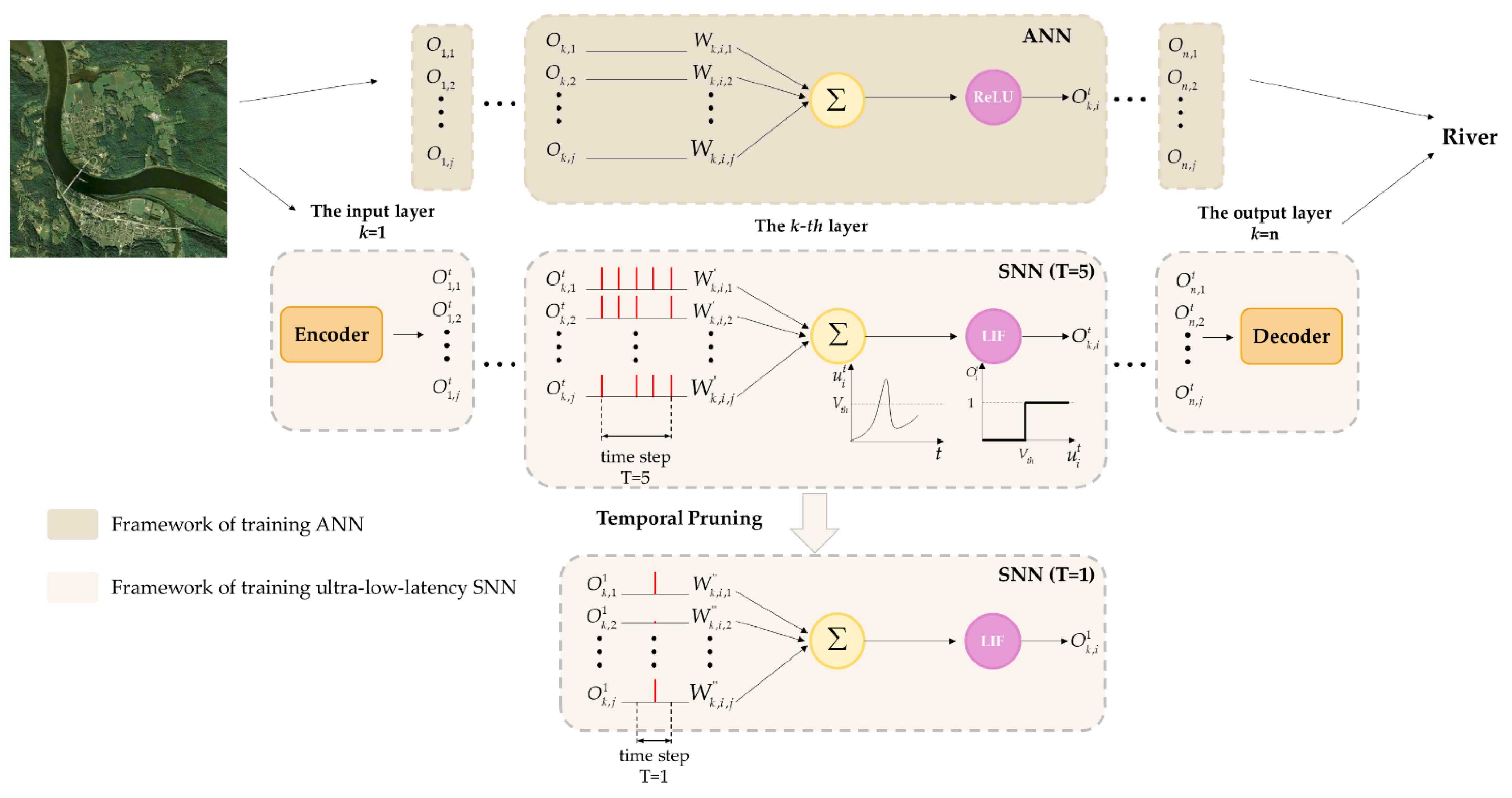
• Inspired by the concept of transfer learning, we introduce a novel spatio-temporal pruning method designed to train ultra-low-latency SNNs. This approach effectively integrates the temporal dynamics characteristic of SNNs with the static feature extraction capabilities of CNNs. Consequently, this method significantly enhances the performances of ultra-low-latency SNNs and effectively reduces the performance gap with ANNs.
• Since residual connections allow information to cross layers, the influence of network structures (such as VGG and ResNet) on feature extraction varies differently. To investigate the effectiveness of our method across different network structures, we analyze the impact of the position of the fundamental module (the module subject to pruning) on feature expression and determine the optimal pruning strategy accordingly.
• To validate the efficacy of our method, we construct an ultra-low-latency SNN training framework based on the leak integrate-and-fire (LIF) neuron model. Through evaluation in a remote sensing scene classification task, our method not only achieves state-of-the-art performance but also successfully reduces the latency of SNNs to one time step, which is 200 times lower than those of other advanced approaches.

The structure of the subsequent sections of this article is organized as follows: Section 2 offers a comprehensive review of three widely employed methodologies utilized in training ultra-low-latency SNNs. In Section 3, we delve into the intricate details of our proposed spatio-temporal pruning method, elucidating its methodology. Section 4 showcases the experimental results, encompassing both performance metrics and energy efficiency, which serve to assess the effectiveness of our proposed method. Finally, Section 5 concludes the paper, summarizing the key findings and implications derived from this study.

2. Related Works

2.1. Remote Sensing Scene Classification

A variety of methods have been proposed for classifying remote sensing scenes over the past few decades. One early approach is the hand-crafted feature-based method, which relies on expert knowledge and technical techniques to define color, texture, scale, and shape attributes for classifying remote sensing images. This method includes the histogram of oriented gradient [24], scale-invariant feature transformation [25], and GIST [26]. However, due to its reliance on researchers’ experience, this traditional method falls short in capturing high-level features, consequently restricting the image description.

Over the past decade, artificial intelligence (AI) techniques, particularly deep learning, have seen significant advancements. Deep learning algorithms, notably convolutional neural networks (CNNs), have demonstrated remarkable feature representation capabilities in a wide range of visual tasks, including remote sensing image classification. In contrast to hand-crafted feature-based methods, deep neural network architectures learn more abstract and distinctive semantic features, leading to superior classification performance [27,28,29,30]. However, with the surge in remote sensing data and rising demand for real-time processing, the challenges associated with the resource and energy consumption of CNNs are becoming increasingly noticeable [31]. To address this issue, some researchers are exploring novel network structures, particularly spiking neural networks. Lossless conversion has been achieved on the UC–Merced data set and WHU-RS dataset [11]. The potential energy consumption benefits of the SNNs for on-board AI applications are investigated theoretically in [32]. Additionally, a spiking neuron threshold-following reset method has been proposed to minimize the loss of conversion [12].

These studies demonstrate that SNNs can attain high-performance classification outcomes in remote sensing scene classification; however, they all depend on utilizing high time steps to maintain network performance. Increased time steps necessitate more time for the network to conduct forward propagation, potentially leading to delayed critical decisions and maintaining the system in a high-energy consumption state. Diverging from prior research efforts, this paper concentrates on developing ultra-low-latency and high-performance spiking neural networks for remote sensing scene classification tasks.

2.2. Methods of Training Ultra-Low-Latency SNNs

Currently, there are three mainstream methods used to train ultra-low-latency SNNs, which are ANN-SNN conversion, direct training, and hybrid training.

2.2.1. ANN-SNN Conversion

The ANN-SNN conversion method replaces rectified linear unit (ReLU) activation in ANNs with a spike activation in SNNs, which matches features between the two domains. Using this method, the parameters of SNNs can be directly informed by ANNs. While previous research has proposed numerous methods to mitigate ANN-SNN conversion errors with promising results, the achieved latency remains unsatisfactory [33,34,35,36,37,38,39]. Consequently, recent studies have conducted more in-depth analyses of error sources to reduce the time step to one [14,15,40]. However, this method does not make use of the time information of SNNs, which limits the method to obtaining ultra-low-latency SNNs with high performance on complex tasks [41].

2.2.2. Direct Training

Direct training utilizes the timing information to train low-latency SNNs. To address the non-differentiable spiking function, optimization based on surrogate gradients has been proposed to achieve low latency and high accuracy [42]. This method has been demonstrated to perform well on both static and dynamic datasets [17,43,44,45]. Furthermore, other researchers have proposed methods based on backpropagation algorithms such as STBP [46], and tdBN [44]. Additionally, to minimize loss, researchers have investigated various approaches from different aspects including basic spiking neurons [39], batch normalization (BN) [47], and learnable membrane time constants [48]. Despite achieving a reduction in latency to around five through direct training methods [49,50], researchers in recent years have conducted further studies to reduce latency while minimizing loss through error analysis and structural design optimization [51,52].

The direct training of ultra-low-latency SNNs is more likely to suffer from gradient vanishing and explosion. Additionally, stochastic initialization random initialization may make the ultra-low-latency SNN unable to receive enough input signals to activate spikes, which in turn affects the network performance.

2.2.3. Hybrid Training

The ANN-SNN conversion and direct training primarily leverage information from the ANN domain and the SNN domain, respectively. In contrast, hybrid training integrates these two approaches by effectively incorporating information from both domains. By employing the hybrid training method, it is feasible to reduce latency and expedite the convergence of direct backpropagation from scratch [53]. The hybrid method involves initially training an ANN and then transferring the trained parameters of the ANN into the SNN [41], similar to the ANN-SNN conversion method. Subsequently, the SNN is trained using surrogate gradients and backpropagation through time. The hybrid training approach utilizing ANN parameters provides several advantages over direct training, including reduced training time and improved operational efficiency. By incorporating surrogate gradients, this method enables the acquisition of distinct temporal information representations in SNNs compared to ANNs. Additionally, the utilization of knowledge distillation methods to train SNNs using ANNs can also be considered as a variant of the hybrid training method [18,54].

The hybrid training has achieved high-performance and ultra-low-latency SNNs on ImageNet. Furthermore, the TP method [13] exemplifies the effectiveness of the hybrid approach by reducing the time step to one while maintaining superior performance. It effectively minimizes the loss between ANNs and SNNs by iteratively decreasing the time step and obtaining high-performance ultra-low-latency SNNs. However, it is important to note that the loss in SNNs is not limited to the temporal domain represented by time steps but also occurs in the spatial domain at different depths. The TP method neglects the issue of reducing the spatial domain loss between ultra-low-latency SNNs and ANNs. To address this gap, this paper proposes a novel spatio-temporal pruning method for training ultra-low-latency SNNs, aiming to compensate for the loss from the spatial perspective. Since our method leverages both the spatial and temporal characteristics of SNNs, it successfully further improves the performances of ultra-low-latency SNNs without changing the given network architecture.

3. Proposed Method

3.1. Overall Workflow of the Proposed Spatio-Temporal Pruning Method

As illustrated in Figure 1, our proposed method was delineated into three distinct phases: (1) ANNa to ANNb, (2) ANNb to SNNb, and (3) SNNb to SNNa. In the first step, fundamental blocks were introduced to compensate for network performance in the spatial domain. This step aimed to enhance the overall performance of the network. The second step employed the temporal pruning method to reduce the latency of SNNs, yielding the Source SNN. The third step involved the strategic removal of the aforementioned blocks via spatial pruning, thereby optimizing the performance of the Target SNN. Since our method combined both temporal and spatial pruning, our method effectively exploited the spatio-temporal characteristics intrinsic to SNNs.

The fundamental blocks played an essential role in the process of our method. We name the blocks as the Unit shown in Figure 1. The location of Units significantly impacted the accuracy of ultra-low-latency SNNs. Figure 1 illustrates two approaches for implementing the proposed method in the spatial domain. Since the number of channels remained the same, adding Units to the shallow layers of the network was advantageous for capturing more detailed features. Conversely, if Units were located in the deeper layers, the network’s ability to improve may have been limited. Therefore, our proposed method compensated for spatial feature extraction by adding Units in the ANN and subsequently removing the corresponding Units in the SNN. Our method was depicted as outlined in Algorithms 1 and 2.

Step 1: ANNa to ANNb. To obtain the new network ANNb, M Units were added to the AS^th layer of the ANNa. This process was denoted as Add_Unit(n,m,N_a) in Algorithm 1. Subsequently, ANNb was trained within the domain of ANN.

Step 2: ANNb to SNNb. The TP method was employed to initialize the SNNb with the parameters of the ANNb. Then, the training process occurred in the SNN domain, with a transition from T = N to T = 1. Finally, the SNNb was obtained with the same time steps as the SNNa, serving as the Source SNN.

Step 3: SNNb to SNNa. Once the added Units were removed from the Source SNN, the network structure aligned with that of the Target SNN. Therefore, this process could be viewed as spatial pruning, as illustrated in Algorithm 2. Meanwhile, this process could be regarded as the inverse procedure from ANNa to ANNb. Subsequently, the Target SNN incorporated the parameters of the layer corresponding to the Source SNN. The Target SNN was then trained to attain the high-performance ultra-low-latency SNN.

Algorithm 1: Spatio-Temporal Pruning Method

Input: the number of Unit (M), the location of Unit (AS), ANN model (Na, Nb), SNN model (Sa, Sb).

for m in M do

if n == AS then // the nth layer is the location of Unit

Nb (n,m) ← Add_Unit(n,m,Na)    // Step1

Sb (n,m) ← Nb (n,m) // TP method;Step2

Sa ← Sb (n,m)                                          // Algorithm 2; Step3

end for

In conclusion, our proposed method effectively enhances the performances of ultra-low-latency SNNs by spatially compensating for network information.

Algorithm 2: Spatial pruning from SNNb to SNNa

Input: the number of layers in Sa (La), SNNa weights (Wa), SNNb weights (Wb), SNNa threshold (va), SNNb threshold vb, SNNa membrane leak (λa), SNNa membrane leak (λb).

for i = 0 in range(La) do

if  i < AS then

Wa [i] ← Wb [i]

va [i] ← vb [i]

λa [i] ← λb [i]

else

Wa [i] ← Wb [i+ M]

va [i] ← vb [i+ M]

λa [i] ← λb [i+ M]

end for

3.2. Deep Networks with the Structure of Unit

The Unit is the fundamental block of a network. The different network was composed of different Units shown in Figure 2. For a VGG-like network in ANNs, a Unit typically consisted of convolutional (Conv), batch normalization (BN), and rectified linear unit (ReLU) layers. However, as the BN layer was eliminated in SNNs, the Unit was described as a combination of convolutional (Conv) and leaky integrate-and-fire (LIF) layers. Similarly, in the ResNet network, the Unit referred to the building block in [55]. In summary, the Unit, as defined in this study, served as the fundamental building block of the network architecture.

3.3. The Framework of Training Ultra-Low-Latency SNNs

Since three steps of our approach have been outlined in Section 3.1, two steps, both ANNb to SNNb and SNNb to SNNa, were dependent on the framework of training ultra-low-latency SNNs. In this section, we introduce our training framework based on the LIF neuron model, as shown in Figure 3.

3.3.1. Spiking Neuron Model

SNNs simulate biological neurons with leaky integrate-and-fire (LIF) layers [56] described as

$$u_{k,i}^t={\lambda }_{k,i}{u}_{k,i}^{t-1}+{\displaystyle \sum _j{w}_{k,i,j}{o}_{k,j}^t}$$

(1)

$$o_{k,i}^{t-1}=\left\{\begin{array}{l}1, \mathrm{if}{u}_{k,i}^{t-1}>v_{k,i}\hfill \\ 0, \mathrm{otherwise}\hfill \end{array}\right.$$

(2)

After the activation of a neuron, the membrane voltage underwent a soft reset, resulting in a new voltage value computed by the following formula:

$$u_{k,i}^t=u_{k,i}^t-v_{k,i}{o}_{k,i}^{t-1}$$

(3)

where u is the membrane potential, λ is the leak constant, and w is the weight connecting pre-neuron j and post-neuron i in the k-th layer. The o is the output in spikes, v is the voltage threshold, and t is the time steps. The formula (3) is written as the following matrix:

$$U_k^t={\lambda }_k{U}_k^{t-1}+W_k{O}_{k-1}^t$$

(4)

$U_k^t$ represents the membrane voltage of the k-th layer at time step t. $W_k$ denotes the k-th layer weight, and $O_{k-1}^t$ denotes the spikes of (k − 1)th layer at time step t. The activation of spikes is as follows:

$$O_k^t=\Theta (U_k^t-V_{th})$$

(5)

$$U_k^t=U_k^t-V_{th}{O}_k^t$$

(6)

where $\Theta$ is the Heaviside step function, and V_th is the voltage threshold.

3.3.2. Surrogate Gradient

For the concept of direct training, the SNN was treated as a recurrent neural network (RNN), enabling the calculation of gradients through spatial–temporal backpropagation (STBP) [46].

$${\displaystyle \frac{\partial L}{\partial W}}={\displaystyle \sum _t\frac{\partial L}{\partial O}\frac{\partial O}{\partial U}\frac{\partial U}{\partial W}}$$

(7)

The term ${\displaystyle \frac{\partial O}{\partial U}}$ is the gradient of the non-differentiability step function involving the derivative of Dirac’s δ-function that is typically replaced by surrogate gradients with a derivable curve. So far, various shapes of surrogate gradients have been identified, such as rectangular [43,46], triangle [41,57], and exponential [45] curves. Here, we selected the surrogate gradient shaped like triangles, which can be described as follows:

$${\displaystyle \frac{\partial O}{\partial U}}=\gamma \max \{0,1-\left|{\displaystyle \frac{U}{V_{th}}}-1\right|\}$$

(8)

where γ is the constant representing the maximum value of the gradient. Moreover, both the threshold and the leak are trainable parameters [41].

3.3.3. Input Layer and Direct Encoding

In the proposed approach, the images were directly fed into the input layer of the SNN at each time step, as indicated in [40,54]. The first convolutional layer, consisting of leaky integrate-and-fire (LIF) neurons, serves a dual purpose by functioning as both a feature extractor and a spike generator. This layer accumulates weighted pixel values and generates output spikes. Given that the first layer transforms the image into spikes, it can be considered a form of direct encoding, as shown in Figure 3.

If the input layer accepted the image as X and output spikes, then the membrane voltage in this layer was

$$U_1^t={\lambda }_1{U}_1^{t-1}+W_{1}X$$

(9)

The weight was updated as follows and ${\displaystyle \frac{\partial O_1}{\partial U_1}}$ is computed using formula (8):

$${\displaystyle \frac{\partial O_1}{\partial W_1}}={\displaystyle \frac{\partial O_1}{\partial U_1}}{\displaystyle \frac{\partial U_1}{\partial W_1}}={\displaystyle \frac{\partial O_1}{\partial U_1}}X$$

(10)

3.3.4. Output Layer and Loss Function

Since LIF neurons were not present in the output layer, no spikes ere generated in this layer. Instead, it received spikes from the previous layer and computed the necessary calculations to produce the output. It could be regarded as the “Decoder”, as shown in Figure 3. The final layer was denoted as the n-th layer, and the formula (6) could be expressed as

$$U_n^t={\lambda }_n{U}_n^{t-1}+W_n{O}_{n-1}^t$$

(11)

The output of the last layer is passed through a SoftMax function to calculate the cross-entropy loss. The weights are then updated using the following formula:

$${\displaystyle \frac{\partial L}{\partial W_n}}={\displaystyle \frac{\partial L}{\partial U_n^t}}{\displaystyle \frac{\partial U_n^t}{\partial W_n}}=(s-y)O_{n-1}^t$$

(12)

where s is the SoftMax values vector, L is the cross-entropy loss function, and y is the one-hot encoded vector of the true label.

3.3.5. Conversion of Batch Normalization Layers

Drawing on the idea of ANN-SNN conversion, we integrated the parameter features of BN into the convolutional layer, where $\sigma$ is the variance, $\mu$ is the mean, $\gamma$ and $\beta$ are learnable parameters.

$$\widehat{W}={\displaystyle \frac{\gamma W}{\sigma }},\widehat{b}={\displaystyle \frac{\gamma (b-\mu )}{\sigma }}+\beta$$

(13)

When selecting the initial training value for the threshold in each layer of an artificial neural network (ANN), directly choosing outliers from the activation function’s output may lead to decreased firing rates and prolonged training time. To address this issue and enhance firing rates while reducing loss, we adopted the approach of selecting the 90.0 percentile of the pre-activation distribution as the threshold in each layer, as previously demonstrated in [58].

3.3.6. Temporal Pruning

As the time steps decrease, spikes may fail to emit at deeper layers, leading to convergence failure. To address this issue, the temporal pruning method started with an SNN of N time steps and gradually reduced the time step with each training iteration until it reached one time step, as shown in Figure 3. This iterative reduction in time steps mitigated the performance loss caused by the vanishing gradients in ultra-low-latency SNNs. However, this method only takes into account the information in the time domain but ignores the spatial aspect. To fully exploit the spatio-temporal characteristics of SNN, we proposed the spatial–temporal pruning method

4. Experiment and Discussion

In this section, we further evaluate the effectiveness of our method in three public remote sensing datasets. Moreover, we evaluate the low power consumption and robustness of our ultra-low-latency SNNs.

4.1. Datasets and Evaluation Metrics

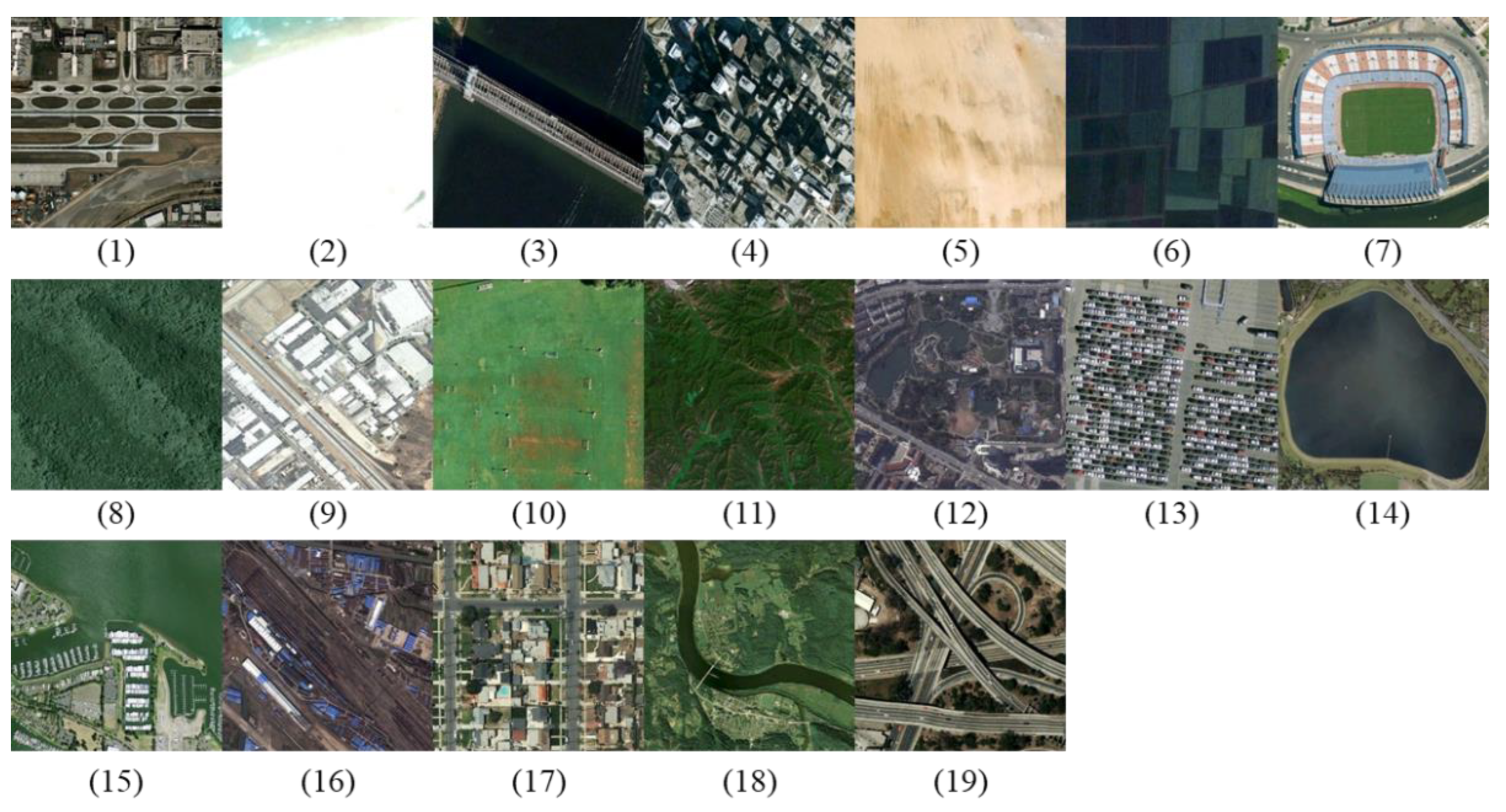
4.1.1. Datasets

Three public datasets in the remote sensing fields are employed to evaluate our method, including the UC–Merced (UCM) dataset, the AID dataset, and the WHU-RS19 dataset.

UC–Merced Dataset: The UC–Merced land-use dataset is from the National Imagery of the United States Geological Survey [59]. The dataset contains a total of 2100 images measuring 256 × 256 pixels and is divided into 21 land-use scene classes, each with 100 images. The size and spatial resolution are 256 × 256 × 3 and 0.3 m. The examples are shown in Figure 4, and the training ratio (TR) is 80%.

AID Dataset: Collecting sample images from Google Earth, AID is a large-scale aerial image dataset containing a total of 10,000 images divided into 30 aerial scene classes [60]. Each class contains from 20 to 420 images with 600 × 600 pixels from 0.5 m to approximately 8 m. The image examples of the dataset are shown in Figure 5. In this paper, we randomly divide the whole dataset at a ratio of 1:1.

WHU-RS19 Dataset: The dataset was released by Wuhan University in 2012. It contains 19 classes and 1005 images in total with 600 × 600 pixels. We randomly select 80% of the whole dataset for training. The image examples are shown in Figure 6.

4.1.2. Evaluation Metrics

In this section, we demonstrate the effectiveness of the method and the advantages of the ultra-low-latency network in terms of performance and energy efficiency.

For performance evaluation, we utilize overall accuracy as a metric to assess classification performance. Overall accuracy is defined as follows:

$$\mathrm{OA}={\displaystyle \frac{N_t}{N_t+N_f}}$$

(14)

N_t and N_f represent the numbers of correctly and incorrectly classified samples.

In terms of energy efficiency, the energy ratio of ANN to SNN α is utilized to assess the energy achieved by low-latency SNNs.

In SNNs, floating-point addition replaces floating-point Multiply–Accumulate (MAC) operations, resulting in a significant reduction in energy consumption. For example, in 45 nm CMOS technology, the energy consumed by a MAC operation is approximately 4.6 pJ, while a floating-point addition consumes only about 0.9 pJ [61]. Consequently, by utilizing a large number of floating-point additions, the energy consumption of SNNs can be at least five times lower than that of ANNs. Since direct coding is employed in this paper, the first layer still retains the operations of ANNs. Therefore, the energy efficiency of the ANN/SNN α in this study is defined as follows:

$$\alpha ={\displaystyle \frac{{\displaystyle {\sum }_{k=1}^L{\mathrm{ANN}}_{\mathrm{FLOPs},k}\times 4.6}}{{\mathrm{SNN}}_{\mathrm{FLOPs},1}\times 4.6+{\displaystyle {\sum }_{k=2}^L{\mathrm{SNN}}_{\mathrm{FLOPs},k}}\times 0.9}}$$

(15)

Considering the sparse spike activity, SNNs do not engage in operations at every moment as ANNs do. To specifically analyze the energy efficiency of SNNs, the firing rate R(k) can be calculated to estimate their energy efficiency.

$$R(k)=\mathbb{E}[{\displaystyle \frac{\#\mathrm{spikes} \mathrm{of} \mathrm{the} k\mathrm{th} \mathrm{layer}}{\#\mathrm{neurons} \mathrm{of} \mathrm{the} k\mathrm{th} \mathrm{layer}}}]\cdot {\displaystyle \frac{1}{T}}$$

(16)

T indicates the time step. The firing rate R(k) reflects the average intensity of the impulse excitation of a single neuron in a single time step.

Hence, ${\mathrm{SNN}}_{\mathrm{FLOPs},k}$ can be obtained using formula (16) as follows:

$${\mathrm{SNN}}_{\mathrm{FLOPs},k}={\mathrm{ANN}}_{\mathrm{FLOPs},k}\times R(k)$$

(17)

${\mathrm{ANN}}_{\mathrm{FLOPs},k}$ and ${\mathrm{SNN}}_{\mathrm{FLOPs},k}$ represent the number of floating-point operations in the k-th layers of the ANN and SNN networks, respectively. To analyze the distribution of spikes across the various layers of the network, we introduce the concept of the spike ratio. This ratio is defined as the proportion of spikes in the k-th layer to the total number of spikes in the network.

$$P(k)=\mathbb{E}[{\displaystyle \frac{\#\mathrm{spikes} \mathrm{of} \mathrm{the} \mathrm{first} k\mathrm{th} \mathrm{layer}}{\#\mathrm{total}\mathrm{spikes} \mathrm{in} \mathrm{all} \mathrm{layers}}}]$$

(18)

4.2. Implementation Details

4.2.1. Networks

To evaluate our method, we select VGG11 and VGG14, as defined in

Table 1. The VGG11 and VGG14 architectures for evaluating the performances of SNNs.

Target SNN	Source SNN	Target SNN	Source SNN
VGG11_Base	VGG11_AS	VGG14_Base	VGG14_AS
conv3-64	conv3-64	conv3-64	conv3-64
		conv3-64	conv3-64
averagepool
conv3-128	conv3-128	conv3-128	conv3-128
		conv3-128	conv3-128
averagepool
conv3-256	conv3-256	conv3-256	conv3-256
conv3-256	conv3-256	conv3-256	conv3-256
		conv3-256	conv3-256
averagepool
conv3-512	conv3-512	conv3-512	conv3-512
conv3-512	conv3-512	conv3-512	conv3-512
		conv3-512	conv3-512
averagepool
conv3-512	conv3-512	conv3-512	conv3-512
conv3-512	conv3-512	conv3-512	conv3-512
	conv3-512	conv3-512	conv3-512
			conv3-512
averagepool
FC-4096		FC-10
FC-4096
FC-10

. For these VGG-like networks, the Unit is ”conv3-X”. The term “3” denotes the size of the convolutional kernel (3 × 3), while “X” indicates the number of channels. In ANNs, “conv3-X” includes a convolutional layer followed by a BN layer and a ReLU layer. In contrast, in SNNs, “conv3-X” refers to a convolutional layer followed by a LIF neuron model. Source SNNs, such as VGG11_AS and VGG14_AS, are optimized architectures designed to achieve high-performance Target SNNs.

Moreover, to assess the impact of the Unit location on the effectiveness of our method, we validate ResNet18 and VGG11 on the UCM dataset and the WHU-RS19 dataset, respectively. The Unit is positioned at different depths within both networks, as defined in

Table 2. The ResNet18 architecture for evaluating the impact of the Unit location.

Target SNN	Source SNN
ResNet18_Base	ResNet18_AS1	ResNet18_AS 2	ResNet18_AS 3	ResNet18_AS 4
conv7-64-2
$\left[\begin{array}{l}3\times 3,64\\ 3\times 3,64\end{array}\right]\times 2$	$\left[\begin{array}{l}3\times 3,64\\ 3\times 3,64\end{array}\right]\times 3$	$\left[\begin{array}{l}3\times 3,64\\ 3\times 3,64\end{array}\right]\times 2$	$\left[\begin{array}{l}3\times 3,64\\ 3\times 3,64\end{array}\right]\times 2$	$\left[\begin{array}{l}3\times 3,64\\ 3\times 3,64\end{array}\right]\times 2$
$\left[\begin{array}{l}3\times 3,128\\ 3\times 3,128\end{array}\right]\times 2$	$\left[\begin{array}{l}3\times 3,128\\ 3\times 3,128\end{array}\right]\times 2$	$\left[\begin{array}{l}3\times 3,128\\ 3\times 3,128\end{array}\right]\times 3$	$\left[\begin{array}{l}3\times 3,128\\ 3\times 3,128\end{array}\right]\times 2$	$\left[\begin{array}{l}3\times 3,128\\ 3\times 3,128\end{array}\right]\times 2$
$\left[\begin{array}{l}3\times 3,256\\ 3\times 3,256\end{array}\right]\times 2$	$\left[\begin{array}{l}3\times 3,256\\ 3\times 3,256\end{array}\right]\times 2$	$\left[\begin{array}{l}3\times 3,256\\ 3\times 3,256\end{array}\right]\times 2$	$\left[\begin{array}{l}3\times 3,256\\ 3\times 3,256\end{array}\right]\times 3$	$\left[\begin{array}{l}3\times 3,256\\ 3\times 3,256\end{array}\right]\times 2$
$\left[\begin{array}{l}3\times 3,512\\ 3\times 3,512\end{array}\right]\times 2$	$\left[\begin{array}{l}3\times 3,512\\ 3\times 3,512\end{array}\right]\times 2$	$\left[\begin{array}{l}3\times 3,512\\ 3\times 3,512\end{array}\right]\times 2$	$\left[\begin{array}{l}3\times 3,512\\ 3\times 3,512\end{array}\right]\times 2$	$\left[\begin{array}{l}3\times 3,512\\ 3\times 3,512\end{array}\right]\times 3$
Adaptive Average pool
FC

and

Table 3. The VGG11 architecture for evaluating the impact of the Unit location.

Target SNN	Source SNN
VGG11_Base	VGG11_AS1	VGG11_AS2	VGG11_AS3	VGG11_AS4	VG11_AS5
conv3-64	conv3-64	conv3-64	conv3-64	conv3-64	conv3-64
	conv3-64
averagepool
conv3-128	conv3-128	conv3-128	conv3-128	conv3-128	conv3-128
		conv3-128
averagepool
conv3-256	conv3-256	conv3-256	conv3-256	conv3-256	conv3-256
conv3-256	conv3-256	conv3-256	conv3-256	conv3-256	conv3-256
			conv3-256	conv3-256
averagepool
conv3-512	conv3-512	conv3-512	conv3-512	conv3-512	conv3-512
conv3-512	conv3-512	conv3-512	conv3-512	conv3-512	conv3-512
				conv3-512
averagepool
conv3-512	conv3-512	conv3-512	conv3-512	conv3-512	conv3-512
conv3-512	conv3-512	conv3-512	conv3-512	conv3-512	conv3-512
					conv3-512
averagepool
FC-4096
FC-4096
FC

. In ResNet18, the Unit corresponds to the building block [55], while in VGG11, the Unit consists of a convolutional layer and an LIF layer, referred to as “conv3-X”.

4.2.2. Hyperparameters Setting

The ANNs are trained using a cross-entropy loss function with stochastic gradient descent optimization that incorporates weight decay (0.0005) and momentum (0.9) parameters. The ANNs are trained for 500 epochs on all datasets with a batch size of 32. The initial learning rate is set to 0.01 and reduced by a factor of 5 at 45%, 70%, and 90% of the total epochs. Dropout is applied with a probability of 0.5. It is noteworthy that the ANNs are trained from scratch.

The SNNs are trained with a dropout probability of 0.2. During the training process, we employ the cross-entropy loss function along with the Adam optimizer with specific parameters, including a weight decay value of 0, a β1 value of 0.9, and a β2 value of 0.99. The SNNs are trained for 300 epochs on all the datasets with a batch size of 8. During the process of moving from ANNb to SNNb, as mentioned in Section 3, an initial learning rate of 0.0001 is selected for each training iteration. This learning rate is divided by a factor of 5 at the 0.6, 0.8, and 0.9 fractions of the total epochs. However, in the process of moving from SNNb to SNNa, since some layers are removed, the learning rate should be relatively higher. The learning rate is 0.0005 and reduced by a factor of 5 at 30%, 60%, 80%, and 90% of the total 300 epochs.

In our experiments, we utilize Python 3.9 and PyTorch 1.12 software and four NVIDIA Titan XP Graphical Processing Units (GPUs). The operating system is Ubuntu 16.04.

To ensure the accuracy of the experiments, all of the experiments are performed five times in each group, and the average and standard deviation of the results of the ten-time experiments are taken as the final experimental results. In order to prevent the order of training and testing samples from affecting the classification results, five different random seeds are chosen for each experiment.

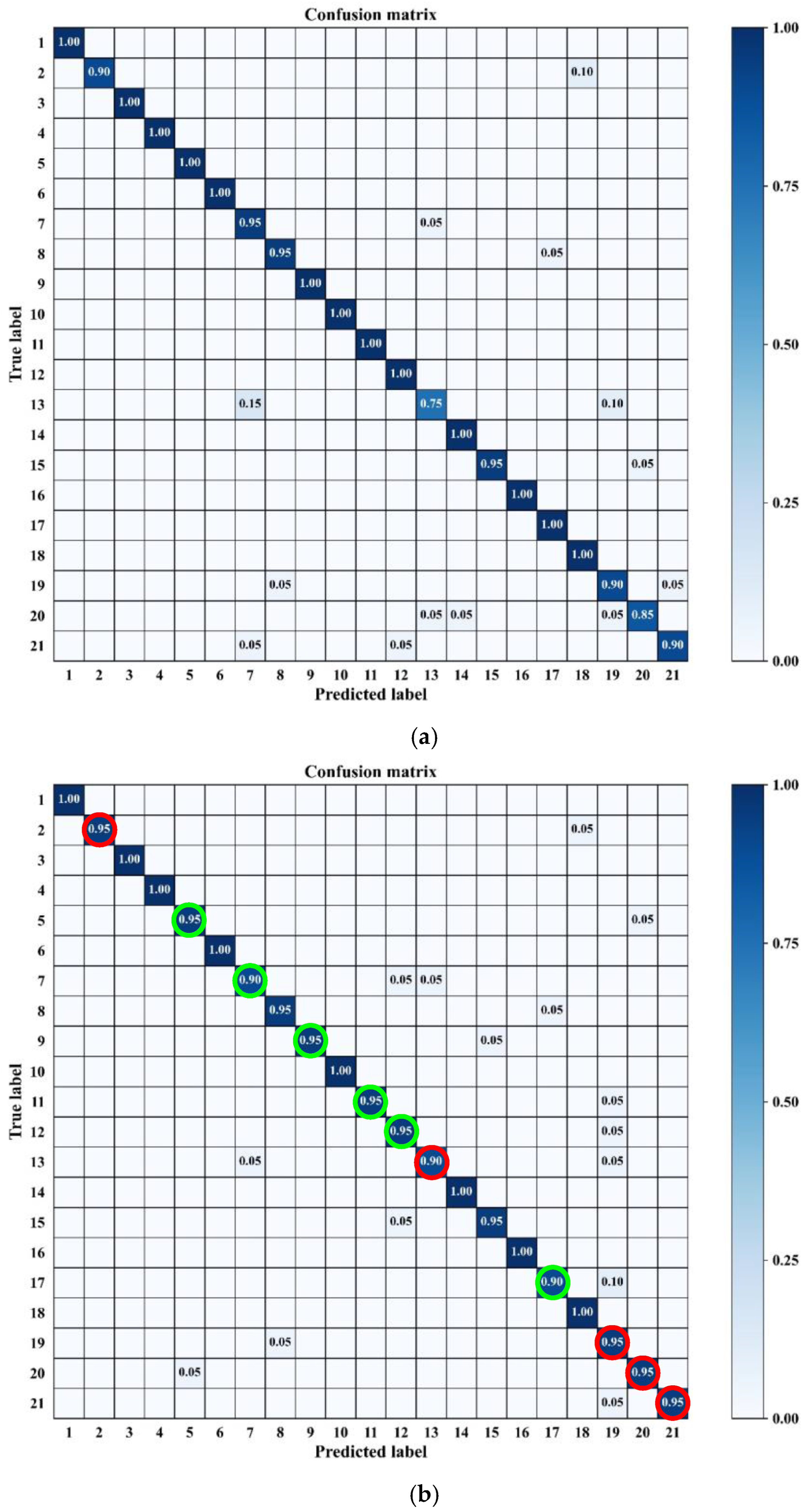
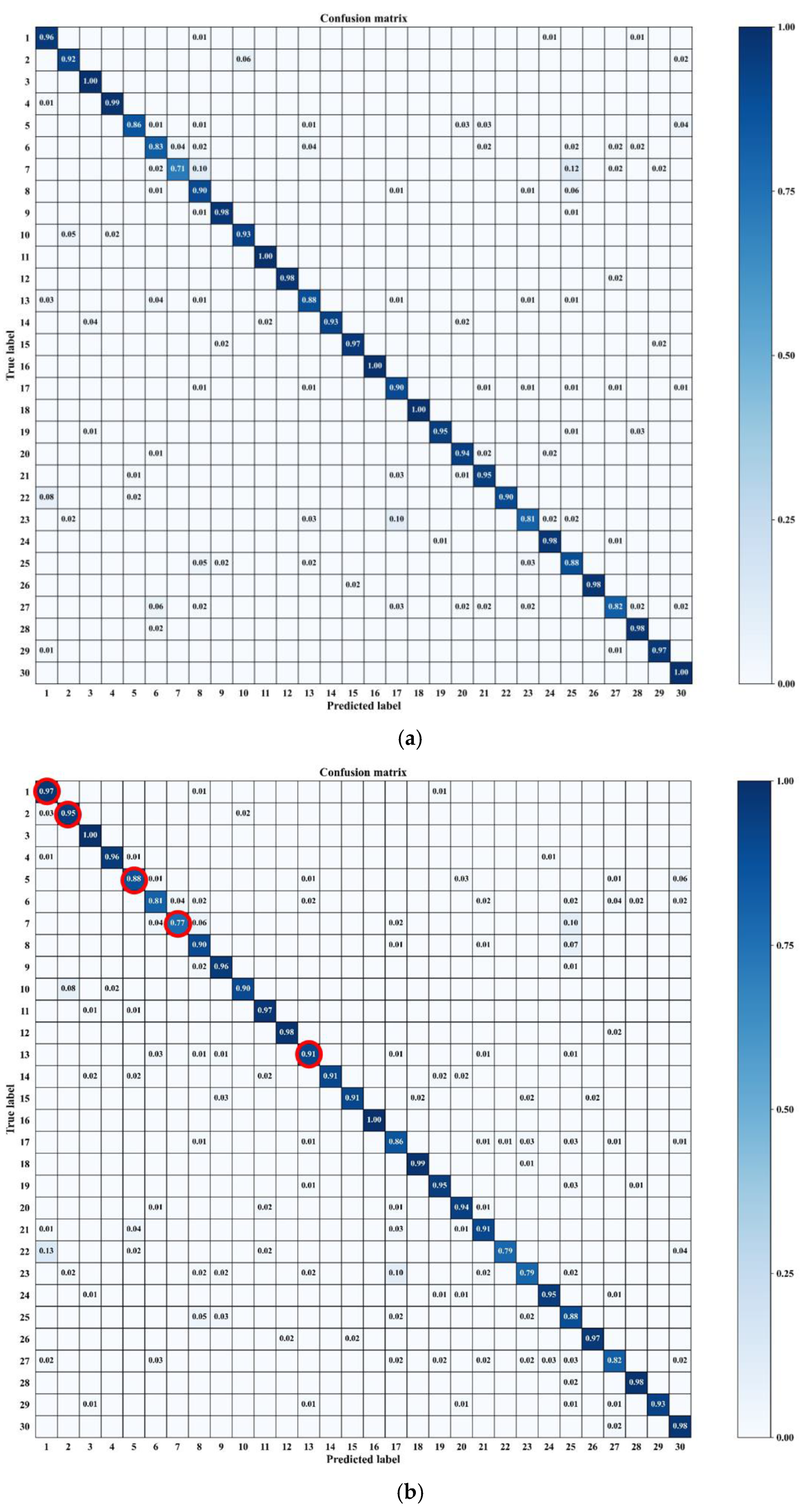
4.3. Experimental Results of Performance

In this section, we first compare ultra-low-latency SNNs and ANNs. The results indicate that, in certain cases, the performances of ultra-low-latency SNNs even surpasses those of ANNs. We then demonstrate that our method achieves state-of-the-art (SOTA) results for ultra-low-latency SNNs compared to other advanced methods. Additionally, the ablation study highlights the effectiveness of our STP method in comparison to the traditional TP method. Furthermore, we demonstrate the optimal network by analyzing the placement of Unit in detail.

4.3.1. Comparison with ANN

The SNN generates spikes, which can be interpreted as quantizing the activation function of the ANN to 1 bit. Consequently, the performance of ultra-low-latency SNNs may experience significant degradation. However, it is important to note that ultra-low-latency SNNs are not always inferior to ANNs; in some cases, they may even surpass ANNs. To provide an objective analysis of this issue, we categorize the evaluation of ultra-low-latency performance into two groups: (1) cases where the OA of the ultra-low-latency SNN is similar to or even higher than that of the ANN, and (2) cases where the OA of the ANN is significantly higher than that of the ultra-low-latency SNN. For the first category, we select VGG14 on the UCM dataset. For the second category, we choose VGG14 on the AID dataset. These comparisons enable us to examine the behavioral differences between ultra-low-latency SNNs and ANNs across various remote sensing categories. The corresponding matrices for these evaluations are illustrated in Figure 7, Figure 8, Figure 9 and Figure 10, respectively.

On the UCM dataset, the performance of the ultra-low-latency SNN closely resembles that of the corresponding ANN, with higher accuracy for specific classes. For the UCM dataset depicted in Figure 7, the SNN outperforms the ANN in categories such as “Airplane”, “Medium Residential”, “Storage Tanks”, “Tennis Court”, and “Mobile Home Park”. Nevertheless, it demonstrates relatively lower accuracy in categories including “Buildings”, “Dense Residential”, “Freeway”, “Harbor”, “Intersection”, and “Runway”. These findings indicate that the ultra-low-latency SNN is not inferior to ANN and exhibits performance advantages in certain scenarios.

In cases where a significant disparity in classification accuracy arises between the ANN and ultra-low-latency SNN, the SNN still demonstrates superior performance in certain scenarios. As illustrated in Figure 8, Figure 9 and Figure 10, the AID training data proportions are 20%, 50%, and 80%, respectively, and the overall accuracy of the ultra-low-latency SNN is lower than that of the ANN by 2.88%, 1.88%, and 1.27%, respectively. When the AID training ratio is 20%, the ultra-low-latency SNN exhibits higher classification accuracy than the ANN in the categories “Beach”, “Center”, “Dense Residential”, “Industrial”, “Park”, and “Parking”, as shown in Figure 8. Similarly, for the training ratio of 50% in Figure 9, the ultra-low-latency SNN outperforms the ANN in the categories “Church”, “Dense Residential”, “Farmland”, “Medium Residential”, and “Playground”. Furthermore, when the AID training ratio is 80%, as shown in in Figure 10, the overall accuracy of the ultra-low-latency SNN surpasses the ANN in the scenarios “Airport”, “Bare Land”, “Bridge”, “Church”, and “Industrial”. Hence, although the overall accuracy of the ultra-low-latency SNN may be lower than that of the ANN, it still exhibits higher accuracy than the ANN in certain categories.

In conclusion, regardless of whether the overall accuracy of the ultra-low-latency SNN is lower or higher than that of the ANN, it outperforms the ANN in certain scenarios. Consequently, the ultra-low-latency SNN has the potential to replace the ANN and achieve higher accuracy in some scenarios.

4.3.2. Comparison with State-of-the-Art Methods

To demonstrate the efficacy of our ultra-low-latency SNNs, we compare our method with other state-of-the-art methods on the UCM and AID datasets. We initialize the network using pretrained parameters, following the approach outlined in [11,12].

Table 4. Comparison of overall accuracy with state-of-the-art methods.

Dataset	Method	Model	Time Step	Accuracy (%)
UCM (TR = 80%)	FACNN [62]	VGG-16(ANN)	-	98.81
	UPetu [63]	ANN	-	99.05
	TF-reset [12]	VGG-15(SNN)	>200	99.00
	Multi-bit spiking [11]	VGG-20(SNN)	>200	98.81
	STP (ours)	VGG-14(SNN)	1	98.81
AID (TR = 80%)	TF-reset [12]	VGG-15(SNN)	>200	94.82
	STP (ours)	VGG-14(SNN)	1	95.6
AID (TR = 50%)	MIDC-Net_CS [64]	ANN	-	92.95
	STP (ours)	VGG-14(SNN)	1	94.72

highlights the advancements achieved by our method. Specifically, our proposed method attains an accuracy equivalent to [12] on the UCM dataset while reducing the number of time steps by a minimum of 200-fold. On the AID dataset, the ultra-low-latency SNN not only achieves a top-1 accuracy that is 0.78% higher than that of [11] but also significantly reduces the number of time steps by at least 200-fold, thereby ensuring real-time processing capabilities.

Additionally, ultra-low-latency SNNs can achieve performance levels comparable to those of ANNs. On the UCM dataset, our ultra-low-latency SNN achieves a top-1 accuracy of 98.81%, which is only 0.24% lower than the results of the state-of-art ANN UPetu [63]. Surprisingly, on the AID dataset, using only 50% of the data for training, our method outperforms the ANN model MIDC-Net_CS [64]. Therefore, our method successfully achieves high-performance and ultra-low-latency SNNs, narrowing the gap with ANNs.

To further validate the effectiveness of our method, we compare it with other methods designed for training ultra-low-latency SNNs. All models are trained from scratch, and the experimental results are presented in

Table 5. Comparison with state-of-the-art methods designed for training ultra-low-latency SNNs.

Dataset	Method	Model	Time Step	Accuracy (%)
UCM (TR = 80%)	IM-Loss [50]	VGG14	2	93.10
	DIET-SNN [41]		2	93.81
	TP [13]		2	94.05
	STP (ours)		2	95.24
WHU-RS19 (TR = 80%)	IM-Loss [50]	VGG11	1	92.37
	DIET-SNN [41]		1	92.86
	TP [13]		1	93.37
	STP (ours)		1	94.9

. On the UCM dataset, our method demonstrates superior performance than the other state-of-the-art methods, achieving a top-1 accuracy of 95.24% with only two time steps using VGG14. A similar trend is observed in the results from the results on the WHU dataset, where our method attains a top-1 accuracy of 94.9% with just one time step, surpassing the performances of other methods. In conclusion, our method can obtain a higher-performance ultra-low-latency spiking neural network in remote sensing scene classification.

4.3.3. Ablation Study

Given that our STP method is derived from the TP method, our ablation study focuses on comparing these two methods. To thoroughly assess the effectiveness of our method, we perform detailed experiments across various models, datasets, and time steps. The experimental outcomes are presented in

Table 6. Classification accuracy of our method on different datasets and networks.

Dataset	Model	Method	SNN T2	SNN T1
UCM (TR = 80%)	VGG14	TP [13]	94.17 ± 1.10	93.89 ± 0.43
	VGG14	STP (ours)	95.33 ± 0.65	95.06 ± 0.69
	ResNet18	TP [13]	93.10 ± 0.45	93.20 ± 0.31
	ResNet18	STP (ours)	93.63 ± 0.35	93.75 ± 0.31
AID (TR = 20%)	VGG11	TP [13]	81.62 ± 0.18	81.37 ± 0.31
	VGG11	STP (ours)	83.48 ± 0.18	83.16 ± 0.17
	ResNet18	TP [13]	76.76 ± 0.16	76.40 ± 0.22
	ResNet18	STP (ours)	77.25 ± 0.24	76.51 ± 0.25

, where “T1” and “T2” designate networks with one time step and two time steps, respectively.

Improvements in performance can be observed on the UCM and AID datasets. Due to the layer-by-layer transmission of features in VGG-like networks, the ability to express features gradually deteriorates as SNN latency is reduced; however, our method effectively compensates for this decline. On the UCM dataset, the STP method outperforms the TP method by approximately 1.2% for SNNs with both one time step and two time steps. Similarly, on the AID dataset, the STP method demonstrates an improvement of about 1.8% compared to the TP method.

However, in ResNet architectures, where features are propagated through skip connections, the feature representation is not strictly constrained by layer-by-layer processing. Consequently, our method shows only limited improvement in ResNet networks. Importantly, our method does not compromise the performances of ResNet networks either.

To facilitate comparison, we present the visualization results obtained through the TP and STP methods using the VGG14 model on the UCM dataset. We analyze the spiking results of all channels in the first layer by selecting representative channel features. As shown in Figure 11, the feature map generated by the TP method exhibits lower intensity, while the overall intensity produced by the STP method is relatively higher. This suggests that the TP method may lead to information loss, whereas the STP method can mitigate such loss. More specifically, the texture features extracted by the TP method appear blurry in Figure 11a, while Figure 11b displays sharper edges and textures. This implies that the STP method is more effective at capturing crucial features such as shape and contour compared to the TP method. Consequently, the STP method compensates for the information loss associated with the TP method and retains intricate texture features.

These significant improvements may stem from several factors. Firstly, the STP method enables the network to leverage the parameters of the deeper network, thereby enhancing its ability to capture image features. Secondly, the deeper layers can result in lower threshold voltages in the initial layer, thereby increasing the likelihood of neurons emitting spikes to retain information.

In summary, the ablation study demonstrates the effectiveness of our approach across various datasets and network architectures. The TP method may hinder the performance of the ultra-low-latency SNN, while our method mitigates this loss from a spatial perspective. It is worth emphasizing that our method solely modifies the network structure during the training phase, without adding any extra complexity. Consequently, it improves the performances of ultra-low-latency SNNs without increasing the overall complexity of the network.

4.3.4. Analysis of Unit Location Impact

The network structure significantly influences feature acquisition. As the position of the Unit alters the network architecture, it also impacts the effectiveness of the proposed method. Therefore, we conduct a systematic analysis to examine the impact of Unit locations on two distinct network structures. ResNet18, recognized for its residual architecture, employs residual connections to propagate features to deeper layers, which contrasts markedly with VGG-like networks. We validate ResNet18 and VGG11 on the UCM and WHU datasets. Units are positioned at various locations within both networks, as detailed in Table 2 and Table 3. The affected side (AS) indicates the location of the Unit to be pruned. In ResNet18, the Unit corresponds to the building block [55], while in VGG11 networks, the Unit comprises a convolutional layer and a LIF layer. Both SNNs operate with one time step. As illustrated in

Table 7. The impact of the Unit location on different networks.

Network	Dataset	Base [13]	AS1	AS2	AS3	AS4	AS5
ResNet18	UCM (TR = 80%)	93.10 ± 0.23	93.75 ± 0.31	93.22 ± 0.26	92.80 ± 0.52	93.04 ± 0.35	-
VGG11	WHU-RS19 (TR = 80%)	92.99 ± 0.66	59.95 ± 0.26	90.06 ± 1.55	89.04 ± 0.85	91.67 ± 0.24	94.26 ± 0.66

, the ”Base” is the results of the TP method without any affected sides.

As illustrated in Table 7, the effectiveness of our method is significantly influenced by the network structure and the position of the Unit. For the VGG11 network, pruning at the AS5 position results in a performance of approximately 94.26%, compared to a baseline performance of 92.99% using the TP method, leading to an improvement of about 1.3%. However, for the ResNet18 network, pruning from the AS1 position yields an OA of 93.75%, which is only about 0.6% higher than the baseline performance. In other pruning positions, our method fails to help both networks to achieve higher performance.

Hence, the placement of the Unit is crucial for the efficacy of the method. In VGG networks, spatial pruning in deeper layers often yields greater enhancements in SNN performance. In contrast, for ResNet networks, our method is inclined to enhance network performance primarily in the context of shallow layers.

4.4. Experimental Results of Energy Efficiency

In this section, we first explain the advantages of low-latency SNNs in terms of their lower power consumption compared to high-latency SNNs. Subsequently, we illustrate the power consumption benefits of low-latency SNNs in comparison to ANNs. To achieve this, we conduct a fair comparison of energy efficiency among SNNs with varying time steps. We carefully select ultra-low-latency SNNs that demonstrate comparable classification accuracy to ANNs. We calculate the total energy ratio of ANN to SNN using the UCM and AID datasets.

As the latency of the SNN increases, the membrane voltage accumulates over multiple time steps, resulting in more spikes and, consequently, greater energy consumption. In other words, as the number of time steps increases, individual neurons are more likely to enter a firing state. We quantify this state of neuronal activity using the firing rate, which is defined by the Equation (16), representing the number of firing pulses per neuron in a single time step. To investigate the activation of ultra-low-latency SNN spikes in remote sensing scene classification tasks, we select deep networks based on the UCM and AID datasets. Specifically, we choose VGG14 and VGG15, each containing 1–2 fully connected layers. Since the last fully connected layer in the network does not include LIF neurons, it does not produce any spikes. Therefore, we only consider neurons that are capable of activating spikes. The results for the firing rate and spike ratio of SNNs with varying time steps are presented in Figure 12 and Figure 13.

With the increase in latency, the firing rate significantly increases in shallow layers but decreases slightly in deep layers. For example, as illustrated in Figure 12 and Figure 13, the firing rate in the first three layers of the network gradually rises from T1 to T3. However, in the last three layers, the firing rate of T1 is higher than that of T2 and T3 in Figure 12 and Figure 13.

In addition, the number of activated spikes in the shallow layers is significantly higher than that in the deep layers. As depicted in Figure 12, the spike ratio in the first four layers is 90.67%, while the spike ratio in the first seven layers is 97.50%. This indicates that the majority of spikes are activated by the shallow layers. Similarly, as shown in Figure 13, the first four layers account for 85.83% of all spikes, and the first seven layers account for 94.83%.

Since the number of spikes activated in the shallow layer greatly exceeds that in the deep layers, the overall network exhibits increased energy consumption as latency rises. In this study, latency does not exceed 3. However, if latency surpasses 200, the energy consumption will increase further. Therefore, compared with networks with more than 200 time steps [11,12], our ultra-low-latency SNN effectively demonstrates the low power consumption that is characteristic of spiking neural networks.

To further investigate the energy consumption of each network layer and explore energy efficiency under different time step conditions, we employ Equation (15) to calculate the energy consumption of each layer. The results are shown in Figure 14.

Since direct coding is employed, the first layer performs a standard convolution operation, resulting in energy consumption at each time step that is equivalent to that of the ANN. Notably, the findings clearly demonstrate that in ultra-low-latency SNNs, energy consumption gradually increases as latency increases. For the VGG14 on the UCM dataset, the energy ratio decreases from 48.06 to 28.50 as T varies from 1 to 3. Similarly, for the VGG15 on the AID dataset, the energy ratio of ANN to SNN decreases from 43.17 to 34.41 as T varies from 1 to 3.

However, the energy consumption of these low-latency SNNs remains significantly lower than that of ANNs by an order of magnitude. This disparity arises from the considerably lower energy consumption at each layer in SNNs compared to ANNs. For example, in the shallower layers, SNNs consume 10 times less energy than ANNs, as shown in Figure 14. Notably, in the deeper layers, SNNs exhibit a remarkable energy reduction of 100 times compared to ANNs. For example, in Figure 14a, at layer 14, the ANN consumes over 10⁷ pJ, while the SNN consumes less than 10⁵ pJ.

In conclusion, ultra-low-latency SNNs effectively leverage the low-power advantages of SNNs, potentially providing a new paradigm for power-constrained scenarios, such as real-time processing for remote sensing satellites.

5. Conclusions

To address the performance degradation caused by reduced latency in ultra-low-latency SNNs, we propose a spatio-temporal pruning training method. This method enhances network performance by adjusting the network structure to compensate for information loss. Through our experiments, we have observed that incorporating fundamental structures, such as the Units described in this paper, can effectively facilitate information compensation in ultra-low-latency SNNs. Specifically, for VGG-like networks, Units in deeper layers are more likely to improve performance. Conversely, for ResNet-like networks, Units in shallower layers can enhance feature extraction. Importantly, our method does not introduce any additional operations to the network architecture, as the pruning of the fundamental structure occurs at the end of the process. We evaluate the effectiveness of our proposed method on remote sensing datasets, achieving competitive results compared to the state-of-the-art approaches. Additionally, we have demonstrated that ultra-low-latency SNNs exhibit lower energy consumption than ANNs. Therefore, our method effectively addresses the challenges associated with reduced latency in ultra-low-latency SNNs, showcasing their potential to advance real-time processing capabilities with improved performance and energy efficiency.

Our evaluation indicates that ultra-low-latency SNNs represent a promising technology with the potential to greatly reduce energy consumption while achieving competitive accuracy levels in specific tasks. This renders them a viable option for various real-time processing applications. We firmly believe that SNNs offer promising technical opportunities for the development of the next generation of real-time processing systems.

References

1. Sang, X.; Xue, L.; Ran, X.; Li, X.; Liu, J.; Liu, Z. Intelligent High-Resolution Geological Mapping Based on SLIC-CNN. ISPRS Int. J. Geo-Inf. 2020, 9, 99. [Google Scholar] [CrossRef]
2. Zhao, W.; Bo, Y.; Chen, J.; Tiede, D.; Blaschke, T.; Emery, W.J. Exploring Semantic Elements for Urban Scene Recognition: Deep Integration of High-Resolution Imagery and OpenStreetMap (OSM). ISPRS J. Photogramm. Remote Sens. 2019, 151, 237–250. [Google Scholar] [CrossRef]
3. Cervone, G.; Sava, E.; Huang, Q.; Schnebele, E.; Harrison, J.; Waters, N. Using Twitter for Tasking Remote-Sensing Data Collection and Damage Assessment: 2013 Boulder Flood Case Study. Int. J. Remote Sens. 2016, 37, 100–124. [Google Scholar] [CrossRef]
4. Cheng, G.; Han, J.; Lu, X. Remote Sensing Image Scene Classification: Benchmark and State of the Art. Proc. IEEE 2017, 105, 1865–1883. [Google Scholar] [CrossRef]
5. Cheng, G.; Yang, C.; Yao, X.; Guo, L.; Han, J. When Deep Learning Meets Metric Learning: Remote Sensing Image Scene Classification via Learning Discriminative CNNs. IEEE Trans. Geosci. Remote Sens. 2018, 56, 2811–2821. [Google Scholar] [CrossRef]
6. Li, E.; Xia, J.; Du, P.; Lin, C.; Samat, A. Integrating Multilayer Features of Convolutional Neural Networks for Remote Sensing Scene Classification. IEEE Trans. Geosci. Remote Sens. 2017, 55, 5653–5665. [Google Scholar] [CrossRef]
7. Zhou, W.; Newsam, S.; Li, C.; Shao, Z. PatternNet: A Benchmark Dataset for Performance Evaluation of Remote Sensing Image Retrieval. ISPRS J. Photogramm. Remote Sens. 2018, 145, 197–209. [Google Scholar] [CrossRef]
8. Maass, W. Networks of Spiking Neurons: The Third Generation of Neural Network Models. Neural Netw. 1997, 10, 1659–1671. [Google Scholar] [CrossRef]
9. Zheng, H.; Wu, Y.; Deng, L.; Hu, Y.; Li, G. Going Deeper with Directly-Trained Larger Spiking Neural Networks. In Proceedings of the AAAI Conference on Artificial Intelligence, Virtually, 2–9 February 2021; Volume 35, pp. 11062–11070. [Google Scholar]
10. Kim, S.; Park, S.; Na, B.; Yoon, S. Spiking-Yolo: Spiking Neural Network for Energy-Efficient Object Detection. In Proceedings of the AAAI Conference on Artificial Intelligence, Midtown, NY, USA, 7–12 February 2020; Volume 34, pp. 11270–11277. [Google Scholar]
11. Wu, S.; Li, J.; Qi, L.; Liu, Z.; Gao, X. Remote Sensing Imagery Scene Classification Based on Spiking Neural Network. In Proceedings of the 2021 IEEE International Geoscience and Remote Sensing Symposium IGARSS, Brussels, Belgium, 11–16 July 2021; pp. 2795–2798. [Google Scholar]
12. Niu, L.-Y.; Wei, Y.; Liu, Y. Event-Driven Spiking Neural Network Based on Membrane Potential Modulation for Remote Sensing Image Classification. Eng. Appl. Artif. Intell. 2023, 123, 106322. [Google Scholar] [CrossRef]
13. Chowdhury, S.S.; Rathi, N.; Roy, K. Towards Ultra Low Latency Spiking Neural Networks for Vision and Sequential Tasks Using Temporal Pruning. In Proceedings of the Computer Vision—ECCV 2022, Tel Aviv, Israel, 23–27 October 2022; Avidan, S., Brostow, G., Cissé, M., Farinella, G.M., Hassner, T., Eds.; Springer Nature: Cham, Switzerland, 2022; pp. 709–726. [Google Scholar]
14. Hao, Z.; Ding, J.; Bu, T.; Huang, T.; Yu, Z. Bridging the Gap between Anns and Snns by Calibrating Offset Spikes. arXiv 2023, arXiv:2302.10685. [Google Scholar]
15. Bu, T.; Fang, W.; Ding, J.; Dai, P.; Yu, Z.; Huang, T. Optimal ANN-SNN Conversion for High-Accuracy and Ultra-Low-Latency Spiking Neural Networks. arXiv 2023, arXiv:2303.04347. [Google Scholar]
16. Guo, Y.; Liu, X.; Chen, Y.; Zhang, L.; Peng, W.; Zhang, Y.; Huang, X.; Ma, Z. Rmp-Loss: Regularizing Membrane Potential Distribution for Spiking Neural Networks. In Proceedings of the IEEE/CVF International Conference on Computer Vision, Paris, France, 2–3 October 2023; pp. 17391–17401. [Google Scholar]
17. Li, Y.; Guo, Y.; Zhang, S.; Deng, S.; Hai, Y.; Gu, S. Differentiable Spike: Rethinking Gradient-Descent for Training Spiking Neural Networks. Adv. Neural Inf. Process. Syst. 2021, 34, 23426–23439. [Google Scholar]
18. Guo, Y.; Peng, W.; Chen, Y.; Zhang, L.; Liu, X.; Huang, X.; Ma, Z. Joint A-SNN: Joint Training of Artificial and Spiking Neural Networks via Self-Distillation and Weight Factorization. Pattern Recognit. 2023, 142, 109639. [Google Scholar] [CrossRef]
19. Chen, H.; Wang, Y.; Xu, C.; Shi, B.; Xu, C.; Tian, Q.; Xu, C. AdderNet: Do We Really Need Multiplications in Deep Learning? In Proceedings of the 2020 IEEE/CVF Conference on Computer Vision and Pattern Recognition (CVPR), Seattle, WA, USA, 13–19 June 2020; pp. 1465–1474. [Google Scholar]
20. Li, W.; Chen, H.; Huang, M.; Chen, X.; Xu, C.; Wang, Y. Winograd Algorithm for Addernet. In Proceedings of the International Conference on Machine Learning, Virtual, 18–24 July 2021; pp. 6307–6315. [Google Scholar]
21. Sakr, C.; Choi, J.; Wang, Z.; Gopalakrishnan, K.; Shanbhag, N. True Gradient-Based Training of Deep Binary Activated Neural Networks via Continuous Binarization. In Proceedings of the 2018 IEEE International Conference on Acoustics, Speech and Signal Processing (ICASSP), Calgary, AB, Canada, 15–20 April 2018; pp. 2346–2350. [Google Scholar]
22. Diffenderfer, J.; Kailkhura, B. Multi-Prize Lottery Ticket Hypothesis: Finding Accurate Binary Neural Networks by Pruning a Randomly Weighted Network. arXiv 2021, arXiv:2103.09377. [Google Scholar]
23. Datta, G.; Liu, Z.; Beerel, P.A. Can We Get the Best of Both Binary Neural Networks and Spiking Neural Networks for Efficient Computer Vision? In Proceedings of the Twelfth International Conference on Learning Representations, Vienna, Austria, 7–11 May 2024. [Google Scholar]
24. Dalal, N.; Triggs, B. Histograms of Oriented Gradients for Human Detection. In Proceedings of the 2005 IEEE Computer Society Conference on Computer Vision and Pattern Recognition (CVPR’05), San Diego, CA, USA, 20–25 June 2005; Volume 1, pp. 886–893. [Google Scholar]
25. Lowe, D.G. Distinctive Image Features from Scale-Invariant Keypoints. Int. J. Comput. Vis. 2004, 60, 91–110. [Google Scholar] [CrossRef]
26. Oliva, A.; Torralba, A. Modeling the Shape of the Scene: A Holistic Representation of the Spatial Envelope. Int. J. Comput. Vis. 2001, 42, 145–175. [Google Scholar] [CrossRef]
27. Zhu, X.X.; Tuia, D.; Mou, L.; Xia, G.-S.; Zhang, L.; Xu, F.; Fraundorfer, F. Deep Learning in Remote Sensing: A Comprehen-sive Review and List of Resources. IEEE Geosci. Remote Sens. Mag. 2017, 5, 8–36. [Google Scholar] [CrossRef]
28. Luus, F.P.; Salmon, B.P.; Van den Bergh, F.; Maharaj, B.T.J. Multiview Deep Learning for Land-Use Classification. IEEE Geo-Sci. Remote Sens. Lett. 2015, 12, 2448–2452. [Google Scholar] [CrossRef]
29. Zhang, F.; Du, B.; Zhang, L. Scene Classification via a Gradient Boosting Random Convolutional Network Framework. IEEE Trans. Geosci. Remote Sens. 2015, 54, 1793–1802. [Google Scholar] [CrossRef]
30. Zhang, W.; Tang, P.; Zhao, L. Remote Sensing Image Scene Classification Using CNN-CapsNet. Remote Sens. 2019, 11, 494. [Google Scholar] [CrossRef]
31. Guo, X.; Hou, B.; Ren, B.; Ren, Z.; Jiao, L. Network Pruning for Remote Sensing Images Classification Based on Interpretable CNNs. IEEE Trans. Geosci. Remote Sens. 2021, 60, 1–15. [Google Scholar] [CrossRef]
32. Kucik, A.S.; Meoni, G. Investigating Spiking Neural Networks for Energy-Efficient on-Board Ai Applications. A Case Study in Land Cover and Land Use Classification. In Proceedings of the IEEE/CVF Conference on Computer Vision and Pattern Recognition, Nashville, TN, USA, 20–25 June 2021; pp. 2020–2030. [Google Scholar]
33. Deng, S.; Gu, S. Optimal Conversion of Conventional Artificial Neural Networks to Spiking Neural Networks. arXiv 2021, arXiv:2103.00476. [Google Scholar]
34. Ding, J.; Yu, Z.; Tian, Y.; Huang, T. Optimal ANN-SNN Conversion for Fast and Accurate Inference in Deep Spiking Neural Networks. In Proceedings of the Thirtieth International Joint Conference on Artificial Intelligence; International Joint Conferences on Artificial Intelligence Organization, Montreal, QC, Canada, 19–27 August 2021; pp. 2328–2336. [Google Scholar]
35. Han, B.; Roy, K. Deep Spiking Neural Network: Energy Efficiency through Time Based Coding. In Proceedings of the European Conference on Computer Vision, Glasgow, UK, 23–28 August 2020; Springer: Berlin/Heidelberg, Germany, 2020; pp. 388–404. [Google Scholar]
36. Li, Y.; Deng, S.; Dong, X.; Gong, R.; Gu, S. A Free Lunch from ANN: Towards Efficient, Accurate Spiking Neural Networks Calibration. In Proceedings of the International Conference on Machine Learning, Virtual, 18–24 July 2021; pp. 6316–6325. [Google Scholar]
37. Yan, Z.; Zhou, J.; Wong, W.-F. Near Lossless Transfer Learning for Spiking Neural Networks. In Proceedings of the AAAI Conference on Artificial Intelligence, Virtual, 2–9 February 2021; Volume 35, pp. 10577–10584. [Google Scholar]
38. Li, Y.; He, X.; Dong, Y.; Kong, Q.; Zeng, Y. Spike Calibration: Fast and Accurate Conversion of Spiking Neural Network for Object Detection and Segmentation. arXiv 2022, arXiv:2207.02702. [Google Scholar]
39. Han, B.; Srinivasan, G.; Roy, K. RMP-SNN: Residual Membrane Potential Neuron for Enabling Deeper High-Accuracy and Low-Latency Spiking Neural Network. In Proceedings of the 2020 IEEE/CVF Conference on Computer Vision and Pattern Recognition (CVPR), Seattle, WA, USA, 13–19 June 2020; pp. 13555–13564. [Google Scholar]
40. Hao, Z.; Bu, T.; Ding, J.; Huang, T.; Yu, Z. Reducing Ann-Snn Conversion Error through Residual Membrane Potential. In Proceedings of the AAAI Conference on Artificial Intelligence, Washington, DC, USA, 7–14 February 2023; Volume 37, pp. 11–21. [Google Scholar]
41. Rathi, N.; Roy, K. Diet-Snn: A Low-Latency Spiking Neural Network with Direct Input Encoding and Leakage and Threshold Optimization. IEEE Trans. Neural Netw. Learn. Syst. 2021, 34, 3174–3182. [Google Scholar] [CrossRef]
42. Neftci, E.O.; Mostafa, H.; Zenke, F. Surrogate Gradient Learning in Spiking Neural Networks: Bringing the Power of Gradient-Based Optimization to Spiking Neural Networks. IEEE Signal Process. Mag. 2019, 36, 51–63. [Google Scholar] [CrossRef]
43. Wu, Y.; Deng, L.; Li, G.; Zhu, J.; Xie, Y.; Shi, L. Direct Training for Spiking Neural Networks: Faster, Larger, Better. In Proceedings of the AAAI Conference on Artificial Intelligence, Honolulu, HI, USA, 27 January–1 February 2019; Volume 33, pp. 1311–1318. [Google Scholar]
44. Zhang, W.; Li, P. Temporal Spike Sequence Learning via Backpropagation for Deep Spiking Neural Networks. Adv. Neural Inf. Process. Syst. 2020, 33, 12022–12033. [Google Scholar]
45. Shrestha, S.B.; Orchard, G. Slayer: Spike Layer Error Reassignment in Time. Adv. Neural Inf. Process. Syst. 2018, 31, 1419–1428. [Google Scholar]
46. Wu, Y.; Deng, L.; Li, G.; Shi, L. Spatio-Temporal Backpropagation for Training High-Performance Spiking Neural Networks. Front. Neurosci. 2018, 12, 323875. [Google Scholar] [CrossRef]
47. Fang, W.; Yu, Z.; Chen, Y.; Masquelier, T.; Huang, T.; Tian, Y. Incorporating Learnable Membrane Time Constant to Enhance Learning of Spiking Neural Networks. In Proceedings of the IEEE/CVF International Conference on Computer Vision, Montreal, BC, Canada, 11–17 October 2021; pp. 2661–2671. [Google Scholar]
48. Kim, Y.; Panda, P. Revisiting Batch Normalization for Training Low-Latency Deep Spiking Neural Networks from Scratch. Front. Neurosci. 2021, 15, 773954. [Google Scholar] [CrossRef]
49. Guo, Y.; Chen, Y.; Zhang, L.; Wang, Y.; Liu, X.; Tong, X.; Ou, Y.; Huang, X.; Ma, Z. Reducing Information Loss for Spiking Neural Networks. In Proceedings of the European Conference on Computer Vision, Tel Aviv, Israel, 23–27 October 2022; Springer: Berlin/Heidelberg, Germany, 2022; pp. 36–52. [Google Scholar]
50. Guo, Y.; Chen, Y.; Zhang, L.; Liu, X.; Wang, Y.; Huang, X.; Ma, Z. IM-Loss: Information Maximization Loss for Spiking Neural Networks. Adv. Neural Inf. Process. Syst. 2022, 35, 156–166. [Google Scholar]
51. Guo, Y.; Tong, X.; Chen, Y.; Zhang, L.; Liu, X.; Ma, Z.; Huang, X. Recdis-Snn: Rectifying Membrane Potential Distribution for Directly Training Spiking Neural Networks. In Proceedings of the IEEE/CVF Conference on Computer Vision and Pattern Recognition, New Orleans, LA, USA, 18–24 June 2022; pp. 326–335. [Google Scholar]
52. Guo, Y.; Zhang, Y.; Chen, Y.; Peng, W.; Liu, X.; Zhang, L.; Huang, X.; Ma, Z. Membrane Potential Batch Normalization for Spiking Neural Networks. In Proceedings of the IEEE/CVF International Conference on Computer Vision, Paris, France, 2–6 October 2023; pp. 19420–19430. [Google Scholar]
53. Rathi, N.; Srinivasan, G.; Panda, P.; Roy, K. Enabling Deep Spiking Neural Networks with Hybrid Conversion and Spike Timing Dependent Backpropagation. arXiv 2020, arXiv:2005.01807. [Google Scholar]
54. Xu, Q.; Li, Y.; Shen, J.; Liu, J.K.; Tang, H.; Pan, G. Constructing Deep Spiking Neural Networks from Artificial Neural Networks with Knowledge Distillation. In Proceedings of the IEEE/CVF Conference on Computer Vision and Pattern Recognition, Vancouver, BC, Canada, 17–24 June 2023; pp. 7886–7895. [Google Scholar]
55. He, K.; Zhang, X.; Ren, S.; Sun, J. Deep Residual Learning for Image Recognition. In Proceedings of the IEEE Conference on Computer Vision and Pattern Recognition, Las Vegas, NV, USA, 26 June–1 July 2016; pp. 770–778. [Google Scholar]
56. Burkitt, A.N. A Review of the Integrate-and-Fire Neuron Model: I. Homogeneous Synaptic Input. Biol. Cybern. 2006, 95, 1–19. [Google Scholar] [CrossRef]
57. Esser, S.K.; Merolla, P.A.; Arthur, J.V.; Cassidy, A.S.; Appuswamy, R.; Andreopoulos, A.; Berg, D.J.; McKinstry, J.L.; Melano, T.; Barch, D.R.; et al. Convolutional Networks for Fast, Energy-Efficient Neuromorphic Computing. Proc. Natl. Acad. Sci. USA 2016, 113, 11441–11446. [Google Scholar] [CrossRef]
58. Rueckauer, B.; Lungu, I.-A.; Hu, Y.; Pfeiffer, M.; Liu, S.-C. Conversion of Continuous-Valued Deep Networks to Efficient Event-Driven Networks for Image Classification. Front. Neurosci. 2017, 11, 294078. [Google Scholar] [CrossRef]
59. Yang, Y.; Newsam, S. Bag-of-Visual-Words and Spatial Extensions for Land-Use Classification. In Proceedings of the 18th SIGSPATIAL International Conference on Advances in Geographic Information Systems, San Jose, CA, USA, 2–5 November 2010; pp. 270–279. [Google Scholar]
60. Xia, G.-S.; Hu, J.; Hu, F.; Shi, B.; Bai, X.; Zhong, Y.; Zhang, L. AID: A Benchmark Dataset for Performance Evaluation of Aerial Scene Classification. IEEE Trans. Geosci. Remote Sens. 2017, 55, 3965–3981. [Google Scholar] [CrossRef]
61. Horowitz, M. 1.1 Computing’s Energy Problem (and What We Can Do about It). In Proceedings of the 2014 IEEE International Solid-State Circuits Conference Digest of Technical Papers (ISSCC), San Francisco, CA, USA, 9–13 February 2014; pp. 10–14. [Google Scholar]
62. Lu, X.; Sun, H.; Zheng, X. A Feature Aggregation Convolutional Neural Network for Remote Sensing Scene Classification. IEEE Trans. Geosci. Remote Sens. 2019, 57, 7894–7906. [Google Scholar] [CrossRef]
63. Dong, Z.; Gu, Y.; Liu, T. UPetu: A Unified Parameter-Efficient Fine-Tuning Framework for Remote Sensing Foundation Model. IEEE Trans. Geosci. Remote Sens. 2024, 62, 5616613. [Google Scholar] [CrossRef]
64. Bi, Q.; Qin, K.; Li, Z.; Zhang, H.; Xu, K.; Xia, G.-S. A Multiple-Instance Densely-Connected ConvNet for Aerial Scene Classification. IEEE Trans. Image Process. 2020, 29, 4911–4926. [Google Scholar] [CrossRef] [PubMed]
Figure 1. The overall workflow of the proposed method. Our method comprises three key steps used to obtain the Target SNN including ANNa to ANNb (Step1), ANNb to SNNb (Step2), and SNNb to SNNa (Step3). T represents time steps. The Unit denotes the fundamental blocks of a network. AS, that is the affected side, represents the location of the Unit. When the SNNb experiences an injury, the parameters of other layers are loaded into the Target SNN correspondingly. Since the added Unit As is removed at the end of our method in Step 3, the underlying network architecture remains unaltered and obtains higher performance.
Remotesensing 16 03200 g001
Figure 2. The illustration of the Unit in the mainstream network architecture.
Remotesensing 16 03200 g002
Figure 3. The framework of training ultra-low-latency SNNs.
Remotesensing 16 03200 g003
Figure 4. Examples in the UCM dataset: (1) Agricultural~100, (2) Airplane~100, (3) Baseball Diamond~100, (4) Beach~100, (5) Buildings~100, (6) Chaparral~100, (7) Dense Residential~100, (8) Forest~100, (9) Freeway~100, (10) Golfcourse~100, (11) Harbor~100, (12) Intersection~100, (13) Medium Residential~100, (14) Overpass~100, (15) Parking Lot~100, (16) River~100, (17) Runway~100, (18) Sparse Residential~100, (19) Storage Tanks~100, (20) Tennis Court~100, and (21) Mobile Home Park~100. (Category~Number of images).
Remotesensing 16 03200 g004
Figure 5. Examples in the AID dataset: (1) Airport~360, (2) Bare Land~310, (3) Baseball Field~220, (4) Beach~400, (5) Bridge~360, (6) Center~260, (7) Church~240, (8) Commercial~350, (9) Dense Residential~410, (10) Desert~300, (11) Farmland~370, (12) Forest~250, (13) Industrial~390, (14) Meadow~280, (15) Medium Residential~290, (16) Mountain~340, (17) Park~350, (18) Parking~390, (19) Playground∼ 370, (20) Pond~420, (21) Port~380, (22) Railway Station~260, (23) Resort~290, (24) River~410, (25) School~300, (26) SparseResidential~300, (27) Square~330, (28) Stadium~290, (29) StorageTanks~360, and (30) Viaduct~420. (Category~Number of images).
Remotesensing 16 03200 g005
Figure 6. Examples in the WHU-RS19 dataset: (1) Airport~55, (2) Beach~50, (3) Bridge~52, (4) Commercial~56, (5) Desert~50, (6) Farmland~50, (7) FootballField~50, (8) Forest~53, (9) Industrial~53, (10) Meadow~61, (11) Moutain~50, (12) Park~50, (13) Parking~50, (14) Pond~54, (15) Port~53, (16) Railwaystation~50, (17) Residential~54, (18) River~56, and (19) Viaduct~58. (Category~Number of images).
Remotesensing 16 03200 g006
Figure 7. The confusion matrix on UCM dataset when the training ratio equals 80%. The semantic names corresonding to different numbers can be found in Figure 4. The red circle indicates that the SNN outperforms the ANN, while the green circle indicates that the SNN is inferior to the ANN. (a) ANN achieves an accuracy of 95.95%. (b) SNN with one time step achieves an accuracy of 96.19%.
Remotesensing 16 03200 g007
Figure 8. The confusion matrix on AID dataset when the training ratio equals 20%. The semantic names corresonding to different numbers can be found in Figure 5. The red circle indicates that the SNN outperforms the ANN. Although SNNs have a lower overall accuracies than ANNs, SNNs still outperform ANNs in some categories, as shown in the red circles. (a) ANN achieves an accuracy of 82.01%. (b) SNN with one time step achieves an accuracy of 79.13%.
Remotesensing 16 03200 g008
Figure 9. The confusion matrix on the AID dataset when the training ratio equals 50%. The red circle indicates that the SNN outperforms the ANN. (a) The ANN achieves an accuracy of 91.74%. (b) The SNN with one time step achieves an accuracy of 89.06%.
Remotesensing 16 03200 g009
Figure 10. The confusion matrix on the AID dataset when the training ratio equals 80%. The red circle indicates that the SNN outperforms the ANN. (a) The ANN achieves an accuracy of 93.4%. (b) The SNN with one time step achieves an accuracy of 92.15%.
Remotesensing 16 03200 g010
Figure 11. A comparison visualization of all the channels of the feature map in the first layer: (a) visualization of feature maps obtained through the traditional TP method; (b) visualization of feature maps obtained through the proposed STP method.
Remotesensing 16 03200 g011
Figure 12. The firing rate and spike ratio of VGG15 on the AID dataset at different latencies.
Remotesensing 16 03200 g012
Figure 13. The firing rate and spike ratio of VGG14 on the UCM dataset at different latencies.
Remotesensing 16 03200 g013
Figure 14. Energy consumption of ultra-low-latency SNNs. (a) VGG14 on the UCM dataset; (b) VGG15 on the AID dataset.
Remotesensing 16 03200 g014