SAR Image Despeckling Based on Denoising Diffusion Probabilistic Model and Swin Transformer

Abstract

The speckle noise inherent in synthetic aperture radar (SAR) imaging has long posed a challenge for SAR data processing, significantly affecting image interpretation and recognition. Recently, deep learning-based SAR speckle removal algorithms have shown promising results. However, most existing algorithms rely on convolutional neural networks (CNN), which may struggle to effectively capture global image information and lead to texture loss. Besides, due to the different characteristics of optical images and synthetic aperture radar (SAR) images, the results of training with simulated SAR data may bring instability to the real-world SAR data denoising. To address these limitations, we propose an innovative approach that integrates swin transformer blocks into the prediction noise network of the denoising diffusion probabilistic model (DDPM). By harnessing DDPM’s robust generative capabilities and the Swin Transformer’s proficiency in extracting global features, our approach aims to suppress speckle while preserving image details and enhancing authenticity. Additionally, we employ a post-processing strategy known as pixel-shuffle down-sampling (PD) refinement to mitigate the adverse effects of training data and the training process, which rely on spatially uncorrelated noise, thereby improving its adaptability to real-world SAR image despeckling scenarios. We conducted experiments using both simulated SAR image datasets and real SAR image datasets, evaluating our algorithm from subjective and objective perspectives. The visual results demonstrate significant improvements in noise suppression and image detail restoration. The objective results demonstrate that our method obtains state-of-the-art performance, which outperforms the second-best method by an average peak signal-to-noise ratio (PSNR) of 0.93 dB and Structural Similarity Index (SSIM) of 0.03, affirming the effectiveness of our approach.

1. Introduction

As an active microwave imaging radar, synthetic aperture radar (SAR) captures high-definition radar images and operates effectively even in low-visibility weather conditions. However, speckle is inherent in all SAR images, primarily caused by image acquisitions, significantly impacting the analysis and interpretation of SAR images [1]. Thus, suppressing speckle noise is crucial to enhancing SAR image quality for subsequent processing tasks. In contrast to Gaussian noise, speckle noise is a multiplicative noise that correlates with spatial and signal characteristics. Over more than 40 years of development, numerous SAR speckle removal algorithms have emerged. The most influential ones can be categorized into three types: local filtering, non-local (NL) filtering, and transform domain filtering.

A local filter chooses a window during filtering noise and filters the pixels inside the window according to the characteristics of the center pixel and its neighboring pixels. Common local filters include the Lee filter [2], the Frost filter [3], the Kuan filter [4], and the Gamma maximum a posteriori (MAP) filter [5]. However, the results of local filter denoising exhibit excessive smoothing and loss of texture.

To mitigate excessive smoothing caused by local filters, filters based on wavelet transform have been developed [6,7,8,9,10]. The typical steps of wavelet denoising involve decomposing the logarithmically transformed SAR image into multiple subband signals using wavelet transform. Subsequently, the wavelet coefficients in the transform domain are adjusted to filter out high-frequency noise components. This process typically employs hard/soft threshold methods. While these transform domain-based speckle removal methods can effectively suppress speckle noise, they may introduce artifacts and pixel distortion.

NL filters have been proposed to overcome the drawbacks of the above-mentioned techniques. Unlike local filters, NL filters no longer rely on neighboring pixels within a defined window. Instead, they search for pixels with similar attributes globally, assign weights to all pixels, and adjust pixel values accordingly. The NL filter has become one of the mainstream algorithms for SAR speckle reduction due to its strong noise suppression ability and preservation of edge information and image details. However, NL filters’ results are highly dependent on parameters, leading to variability in the quality of denoised images. Common NL filters include the probabilistic patch-based (PPB) [11], SAR block-matching 3-D (SAR-BM3D) [12], NL-SAR [13], and fast adaptive nonlocal SAR (FANS) [14].

In recent years, deep learning techniques have been widely applied in low-level visual tasks [15,16], showcasing their advantages in image denoising tasks. Therefore, deep learning-based SAR despeckling methods are gradually emerging and gaining recognition. SAR-CNN [17] utilizes a residual convolutional neural network (CNN) to remove noise from SAR images, marking the first deep learning algorithm for SAR speckle reduction. Subsequently, the ID-CNN [18] introduces a mixed loss function and incorporates total variation (TV) loss to enhance edge information preservation in despeckling results. The multi-objective network (MONet) [19] provides a detailed analysis of the statistical characteristics of SAR speckles, proposing a multi-objective network and integrating Kullback Leibler (KL) divergence to better align with the statistical characteristics of SAR speckles. The dilated residual network (DRN) can increase the receptive field and extract image features more comprehensively, applied in SAR speckle reduction tasks as SAR-DRN [20]. With the proposal of transformer [21], attention mechanisms have been applied to SAR speckle removal tasks. SAR transformer [22] introduces a transformer-based network structure to capture global information effectively. Variable attention modules are employed by SAR-CAM [23], which has shown promising results in removing SAR speckles.

The emergence of generative adversarial networks (GAN) [24] has introduced new concepts to deep learning SAR despeckling. GAN effectively establishes a relationship between generated data and interpretable naturalness through adversarial training of generators and discriminators, thereby enhancing the realism of generated data. Furthermore, the generator’s input data is a hidden vector sampled from a Gaussian distribution, introducing a degree of randomness that enhances the diversity of generated samples, thereby benefiting SAR speckle removal tasks [25,26,27]. The algorithm proposed in [27] applies the GAN concept to construct a network to address speckle noise suppression and detail preservation in homomorphic regions. The rise of denoising diffusion probabilistic model (DDPM) has reignited research interest in Generative Models, and its powerful generative ability has also been applied to SAR speckle reduction and achieving good results [28]. In addition, due to the lack of clean SAR images in the real world, many semi-supervised and self-supervised learning methods for SAR despeckling have been proposed in recent years. SAR2SAR [29] is based on a typical denoising framework called Noise2Noise, which is trained on SAR image pairs from the same scene and fine-tuned on multitemporal SAR images. However, when training with multitemporal SAR images, significant changes may occur in certain areas of the image pairs. To solve this problem, the NR-SAR-DL method [30] improved the training process by considering the similarity of each pixel pair between the different images. Moreover, MERLIN [31] extracted the real and imaginary parts of single-look complex (SLC) images as SAR speckle image pairs for training. Unlike the above methods, Speckle2void [32] is based on a Noise2Void framework, which employed blind-spot CNNs to achieve single image denoising.

However, while the abovementioned methods exhibit good noise suppression effects, they necessitate complex parameter adjustments to achieve the desired visual outcome. In addition, since most algorithms are trained on simulated SAR images assuming independent noise, their denoising efficacy on real SAR images is compromised. Furthermore, there is limited research in the field of SAR speckle removal that combines generative models, leaving their potential largely untapped. SAR-DDPM has demonstrated for the first time the feasibility of applying DDPM to SAR denoising tasks, and in most cases, good denoising results can be obtained. However, due to the use of optical images multiplied by simulated speckles during training, the image structure is different from SAR images, so the DDPM model may result in unstable generation results, leading to overfitting of real-world SAR image denoising results and errors in generating local image regions. To address these challenges, we propose a despeckling algorithm based on the DDPM framework, which utilizes its powerful generative ability to ensure the authenticity of the results and incorporates Swin Transformer to extract global features and enhance detail preservation. Lastly, employing a PD refinement process enables our algorithm to improve performance on real-world SAR data. In comparison to other despeckling methods, our method maintains the excellent visual effect of the DDPM model in image denoising results while reducing the problems of some local generation errors and unstable denoising results for real-world SAR images caused by simulated image datasets, and the effect is particularly prominent in complex texture areas, such as artificial buildings. The main contributions and innovations of this article are as follows:

(1)

We propose a SAR denoising algorithm based on the DDPM framework, which enhances the authenticity of the results with its powerful generation ability. The prediction network in the DDPM reverse diffusion process has been customized to better suit SAR despeckling tasks. Additionally, the network adopts a mixed-loss function aimed at effectively suppressing speckles while preserving the texture and details of the image.

(2)

We integrated the Swin Transformer Block into the U-net network used in DDPM, harnessing the Swin Transformer’s strong capability to extract contextual information. This integration enhances our network’s capacity to extract local and global features effectively.

(3)

We implemented a strategy known as PD refinement during the post-processing stage to mitigate the adverse effects of Gaussian white noise, which is typically used in simulated images and DDPM training. This method aims to enhance the algorithm’s capacity to adapt to SAR speckle noise in actual scenarios.

The remaining part of this article is organized as follows: Section 2 outlines the SAR speckle model and denoising diffusion probabilistic model. An introduction of our proposed method along with its detailed explanation will be provided in Section 3. Section 4 covers the experimental design and compares and analyzes the results with other methods. Morever, the functions of some vital components of the proposed method are thoroughly examined in Section 4. Finally, Section 5 provides a summary of the article.

2. Related Works

2.1. SAR Speckle Model

The surface of ground targets emitted by radar waves is usually rough and contains numerous scattering points. When the SAR system continuously observes the same ground target, the movement process will cause a change in the phase of the scattering points, resulting in the phenomenon of radar wave signal fading. Due to the imaging mechanism based on the principle of coherence in SAR systems, scattered signals exhibit random characteristics and speckle noise in SAR images. To suppress speckles in SAR images, it is necessary first to establish a suitable statistical distribution model. Generally speaking, fully developed coherent speckle noise is spatially and signal-related multiplicative noise [33], which can be mathematically expressed as:

$$X=Y\cdot N$$

(1)

where $N$ represents the speckle noise generated during SAR imaging, $X$ represents the SAR image contaminated by speckle noise, and $Y$ represents the ideal observation value without speckle noise interference.

The speckle noise intensity $N$ of SAR images follows a Gamma distribution with a mean of 1 and a variance of $1/L$. Therefore, the probability density function $P\left(N\right)$ of $N$ can be expressed as:

$$P(N)={\displaystyle \frac{L^L{N}^{L-1}{e}^{-LN}}{\mathsf{\Gamma }(L)}}$$

(2)

where $L$ denotes equivalent Number of Looks (ENL), $\mathsf{\Gamma }$ denotes Gamma function.

According to Equations (1) and (2), we can simulate speckle noise with varying looks $L$ and multiply it with clean images to simulate SAR noise images, thereby enriching the training data for our model.

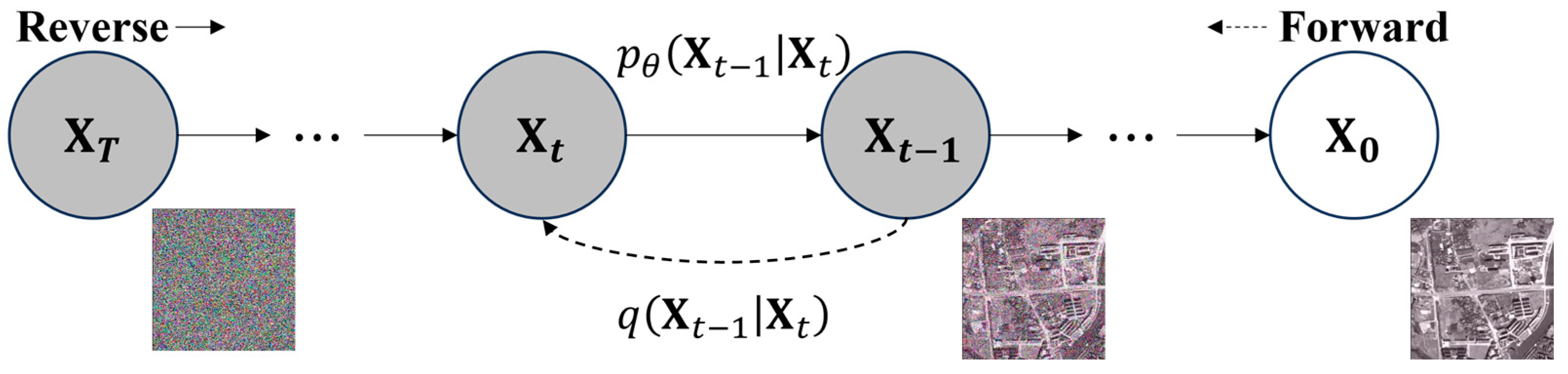
2.2. Denoising Diffusion Probabilistic Model

As a Markov chain process, the diffusion process adds random noise to the clean image ${\beta }_t\in (0,1)$ at various time steps $t$, $t\in \left\{1,2,\dots ,T\right\}$, gradually transforming it into Gaussian white noise $x_T$, which is known as the forward diffusion process. On the contrary, it gradually denoises $x_T$ until a clean image $x_0$ is restored, which is known as the reverse diffusion process. The approximate process can be seen in Figure 1.

The forward propagation process of the diffusion model gradually adds Gaussian noise to the data according to a variance schedule ${\beta }_1,\dots ,{\beta }_T$. Based on the characteristics of Markov chains, $x_t$ can be obtained from $x_{t-1}$ in the forward process:

$$x_t=\sqrt{1-{\beta }_t}{x}_{t-1}+\sqrt{{\beta }_t}{ϵ}_t$$

(3)

where ${\beta }_t\in (0,1)$, and ${ϵ}_t\sim \mathcal{N}(0,1)$. From Equation (3), it can be seen that the generation of $x_t$ only depends on $x_{t-1}$ and is independent of $x_0$. Therefore, there is

$$x_t\sim q(x_t|x_{t-1})=\mathcal{N}(x_t;\sqrt{1-{\beta }_t}{x}_{t-1},{\beta }_{t}I)$$

(4)

In addition, the forward process can be represented as:

$$q(x_{1:T}|x_0):={\displaystyle \prod _{t=1}^T}q(x_t|x_{t-1})$$

(5)

A good property of the forward process is that it admits sampling $x_t$ at an arbitrary timestep $t$ by setting ${\alpha }_t=1-{\beta }_t$ and $\overline{{\alpha }_t}={\displaystyle \prod _{t=1}^T}{\alpha }_i$, we have

$$q(x_t|x_0)=\mathcal{N}(x_t;\sqrt{{\overline{\alpha }}_t}{x}_0,(1-{\overline{\alpha }}_t)I)$$

(6)

The backpropagation process is still a Markov chain, and neural networks are used to predict the parameters of ${\mu }_{\theta }(x_t,t)$ and ${\Sigma }_{\theta }(x_t,t)$:

$$p_{\theta }(x_{0:T}):=p(x_T)\prod _{t=1}^T{p}_{\theta }(x_{t-1}|x_t),$$

(7)

$$p_{\theta }(x_{t-1}|x_t):=\mathcal{N}(x_{t-1};{\mu }_{\theta }(x_t,t),{\Sigma }_{\theta }(x_t,t))$$

(8)

To train the model, we should optimize the usual variational bound on negative log-likelihood:

$$\mathbb{E}[-\log p_{\theta }(x_0)]\le {\mathbb{E}}_q\left[-\log {\displaystyle \frac{p_{\theta }(x_{0:T})}{q(x_{1:T}|x_0)}}\right]={\mathbb{E}}_q{\left[-\log p(x_T)-\sum _{t\ge 1}\log {\displaystyle \frac{p_{\theta }(x_{t-1}|x_t)}{q(x_t|x_{t-1})}}\right]}^{\leftarrow }$$

(9)

Variance can be reduced by rewriting (9) as:

$${\mathbb{E}}_q[\underset{L_T}{D_{\mathrm{KL}}(q(x_T|x_0)\parallel p(x_T))}+\sum _{t>1}\underset{L_{t-1}}{D_{\mathrm{KL}}(q(x_{t-1}|x_t,x_0)\parallel p_{\theta }(x_{t-1}|x_t))}\underset{L_0}{-\log p_{\theta }(x_0|x_1)}]$$

(10)

where $L_{t-1}$ is the KL divergence used to evaluate the similarity between two Gaussian distributions. Here, it is expressed as a probability density of $p_{\theta }(x_{t-1}|x_t)$. And forward process posters expressed as a probability density:

$$q(x_{t-1}|x_t,x_0)=\mathcal{N}(x_{t-1};{\tilde{\mu }}_t(x_t,x_0),{\tilde{\beta }}_{t}I),$$

(11)

$$\mathrm{where} {\tilde{\mu }}_t(x_t,x_0):={\displaystyle \frac{\sqrt{{\alpha }_{t-1}{\beta }_t}}{1-{\overline{\alpha }}_t}}{x}_0+{\displaystyle \frac{\sqrt{{\alpha }_t(1-{\alpha }_{t-1})}}{1-{\overline{\alpha }}_t}}{x}_t \mathrm{and} {\tilde{\beta }}_t:={\displaystyle \frac{1-{\alpha }_{t-1}}{1-{\overline{\alpha }}_t}}{\beta }_t$$

(12)

Since $x_t$ is available as input to the model, we can choose the parameterization strategy for the mean ${\mu }_{\theta }(x_t,t)$ as follows:

$${\mu }_{\theta }(x_t,t)={\displaystyle \frac{1}{\sqrt{{\alpha }_t}}}(x_t-{\displaystyle \frac{{\beta }_t}{\sqrt{1-{\overline{\alpha }}_t}}}{ϵ}_{\theta }(x_t,t))$$

(13)

where ${ϵ}_{\theta }$ is a function approximator intended to predict $ϵ$.

By combining Equation (13) with the gradient descent method, we can obtain the final optimization objective of DDPM:

$$L=||ϵ-{ϵ}_{\theta }(\sqrt{{\overline{\alpha }}_t}{x}_0+\sqrt{1-{\overline{\alpha }}_t}ϵ)|{|}^2$$

(14)

3. Methodology

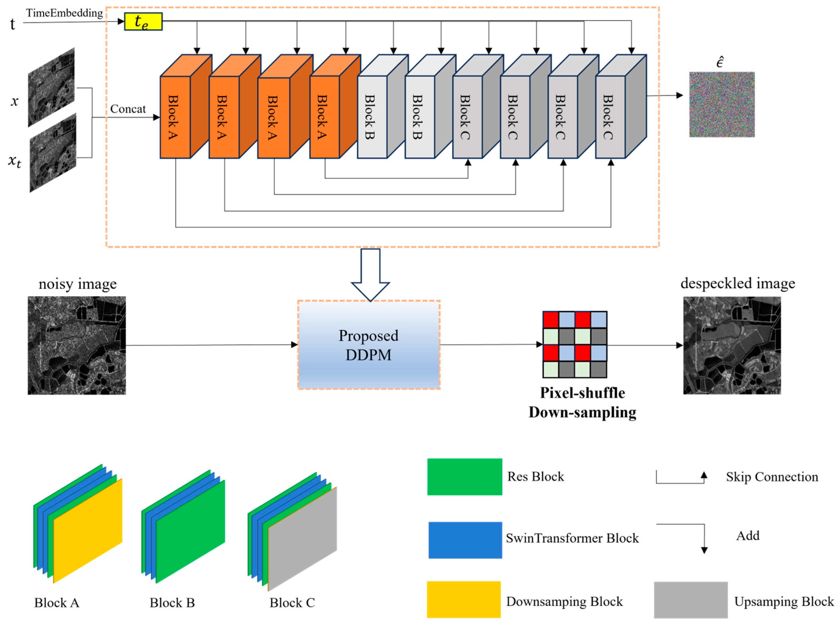
3.1. General Architecture

The despeckling algorithm proposed in this article is based on the denoising diffusion model framework. The proposed diffusion model will be trained to predict noise $\widehat{ϵ}$ during the training phase. During the inference phase, noise images are inputted into the trained model, and a PD refinement process is performed to obtain prediction results. The main structure is shown in Figure 2. The diffusion process consists of two stages: forward propagation and reverse propagation. In the forward propagation process, the optical image serves as the input image $x_0$. Then, Gaussian noise was gradually added to $x_0$ to obtain $x_t$. In the backward propagation, the conditional noise predictor ${ϵ}_{\theta }$ is employed to predict the Gaussian noise added in the forward propagation, thereby recovering $x_0$ from $x_t$.

The proposed prediction network follows a U-net framework, integrating Swin Transformer blocks, residual blocks, upsampling blocks, downsampling blocks, skip connections, and TimeEmbedding layers. In the training phase, the noisy images $x$ and $x_t$ are first connected as input data. We replace the original self-attention blocks with Swin Transformer blocks and use residual blocks from BigGAN [34] as upsampling and downsampling blocks. Simultaneously, the timesteps $t$ were converted to $t_e$ and then added into each residual block via the position encoding process [21]. Finally, the network ultimately outputs the predicted noise $\widehat{ϵ}$ at $t-1$ time steps and use Equations (9) and (13) to obtain $x_{t-1}$. The algorithms for training and sampling in the network are detailed in Algorithms 1 and 2.

Algorithm 1 Traing a denoising model ${ϵ}_{\theta }$

1: repeat

2:   $(x,x_0)\sim q(x,x_0)$ 3:   $t\sim \mathrm{Uniform}(\{1,\dots ,T\})$ 4:   $ϵ\sim \mathcal{N}(0,I)$ 5:   Take gradient descent step on ${\nabla }_{\theta }||ϵ-{ϵ}_{\theta }(x_t,x,t)|{|}^2$ 6: until converged

Algorithm 2 Samping

1: $x_t\sim \mathcal{N}(0,I)$

2: for t = T, …, 1 do 3:   $z\sim \mathcal{N}(0,I)$ if t > 1, else $z=0$ 4:   $x_{t-1}={\displaystyle \frac{1}{\sqrt{{\alpha }_t}}}(x_t-{\displaystyle \frac{1-{\alpha }_t}{\sqrt{1-{\alpha }_t}}}{ϵ}_{\theta }(x,x_t,t))+\sqrt{1-{\alpha }_t}z$ 5: end for 6: return ${\mathit{x}}_0$

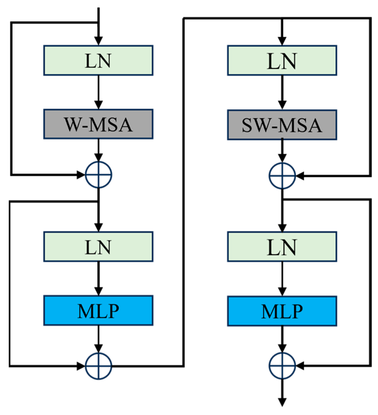
3.2. Swin Transformer Block

We integrated the swin transformer block into the existing DDPM U-net framework to enhance the network’s ability to capture global dependencies. The Swin Transformer block is structured in a two-stage series structure, as illustrated in Figure 3. The first stage uses Window-based multi-head self-attention (W-MSA), and the second uses shifted Window-based multi-head self-attention (SW-MSA). The choice between the two self-attention methods depends on whether the current Swin Transformer Block is odd or even. W-MSA is a windowed multi-head self-attention that reduces a significant amount of computation compared to global self-attention. However, W-MSA can only focus on the content of the windows itself and does not allow cross-window connections, which means that information cannot be transmitted between windows. By shifting windows, SW-MSA introduces cross-window connections that maintain efficient computation of non-overlapping windows. Our multi-head attention consists of three heads, and the window size used in W-MSA is 8. In addition, the input image is divided into non-overlapping patches using the patch partition structure and then merged into a hierarchical representation using the patch merging layer. We posit that the advantage of swin transformer for SAR image speckling tasks lies in its superior structure, which enables it to capture both local features of the image like CNN and contextual information like transformer. This allows both global modeling and effective local information extraction.

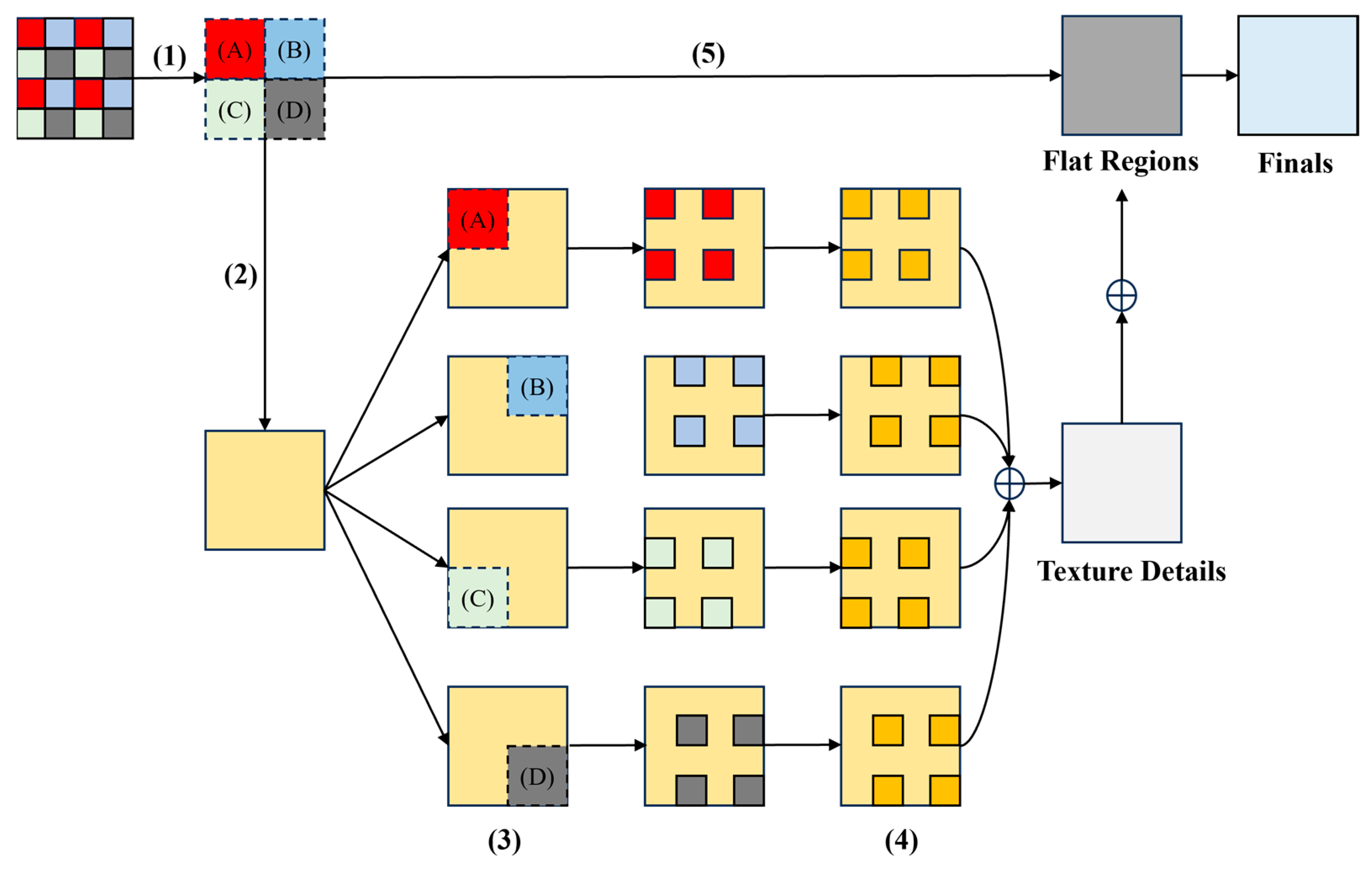
3.3. Pixel-Shuffle Down-Sampling

Due to the lack of clean SAR images in the real world, we generated a training set based on speckle models to simulate speckle noise, and the simulated noise is spatially independent. However, the speckle in real-world SAR images is spatially correlated. To make our method more adaptable to real-world SAR noise, we added the pixel-shuffle down-sampling refinement post-processing strategy to increase robustness. The process of pixel-shuffle down-sampling refinement can be seen in Figure 4. The specific process is as follows:

• Use the stride s, which is 2 in our method, to pixel-shuffle the image into a mosaic $y$. By doing so, we can eliminate noise correlation by dividing adjacent pixels into different small images. When the down sampling rate is high, spectral aliasing and edge loss may occur, so we choose a small number of s;
• Despeckle $y$
• Refill each sub-image with speckle image blocks separately, and pixel-shuffle up sample them;
• Despeckle each refilled image again and average them;
• Combining the details and texture information from speckled images with over-smoothed regions.

3.4. Loss Function

Our method employs a mixed loss function to balance the statistical characteristics, spatial features, and human perception in denoising SAR images. Consequently, the final loss function is a combination of three different losses:

$$\mathcal{L}={\mathcal{L}}_1+{\mathcal{L}}_{\mathrm{KL}}+{\lambda }_{\mathrm{TV}}{\mathcal{L}}_{\mathrm{TV}}$$

(15)

Next, we will elaborate on each loss function in detail.

3.4.1. L1 Loss

Most deep learning-based image denoising algorithms use the l2 or mean squared error (MSE) loss function because minimizing the l2 loss function is consistent with maximizing the PSNR. Therefore, deep learning denoising algorithms based on the l2 loss function often achieve good results on the PSNR metric. However, the PSNR metric is not entirely consistent with our human visual perception. In addition, due to the inherent characteristics of the MSE loss function, removing speckle noise will inevitably lead to the blurring of texture details and excessive smoothing of edges. On the contrary, deep learning models based on the l1 loss function can obtain images with relatively more precise edges. The L1 loss can be calculated as follows:

$${\mathcal{L}}_1=\parallel Y-X\parallel$$

(16)

where $Y$ represents the denoised image, and $X$ represents the noisy image.

3.4.2. KL Loss

Kullback Leibler diversity ($D_{KL}$) is used to measure the similarity between two statistical measures. In our method, we choose to compare the distribution of estimated noise $\widehat{N}$ and theoretical noise $N$ same as [19]:

$${\mathcal{L}}_{\mathrm{KL}}=D_{\mathrm{KL}}(\widehat{N},N)=\sum _i{P}_{\widehat{N}}(i){\log }_2\left({\displaystyle \frac{P_{\widehat{N}}(i)}{P_N(i)}}\right)$$

(17)

where $P_{\widehat{N}}$ denotes pdf of $\widehat{N}$ and $P_N$ denotes pdf of $N$.

3.4.3. TV Loss

Total variation loss is a commonly used loss function in noise reduction tasks. The difference in adjacent pixel values in an image can be solved to a certain extent by reducing TV loss, thereby maintaining the image’s smoothness. Its expression is as follows:

$${\mathcal{L}}_{\mathrm{TV}}=\sum \sqrt{{\left(x_{i,j-1}-x_{i,j}\right)}^2+{\left(x_{i+1,j+1}-x_{i,j+1}\right)}^2}$$

(18)

where $x$ denotes pixel values in images. Considering the order of magnitude difference between TV loss and other losses, ${\mathcal{L}}_{\mathrm{TV}}$ must be multiplied by a weight. After experiments, we chose the optimal weight ${\lambda }_{\mathrm{TV}}$ as 1 × 10⁻⁴.

4. Experiments and Results

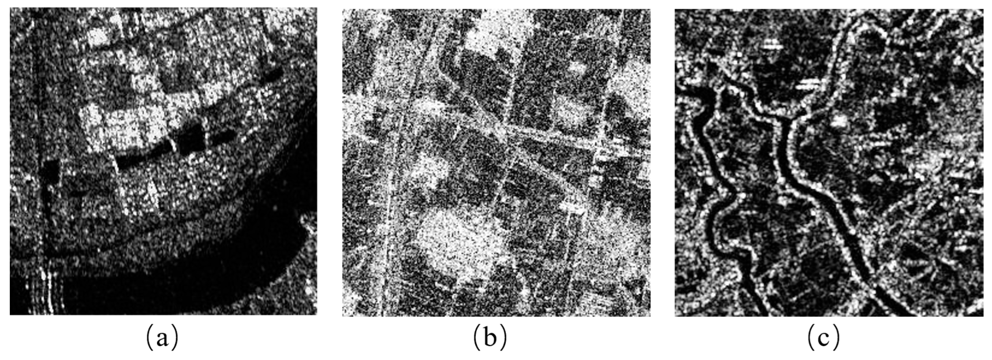
4.1. Datasets

Optical remote sensing images are frequently employed to train SAR image speckle removal models because they typically lack multiplicative noise, which is prevalent in SAR images. In addition, optical images generally exhibit low noise levels and high spatial resolution characteristics, which means that using them to train SAR denoising models will yield more accurate results. The similarity between optical images and SAR images enables the trained SAR speckle removal model to perform better on real-world images. Therefore, we used DSIFN datasets [35] as our training data. The dataset consists of six large, high-resolution images covering six cities (i.e., Beijing, Chengdu, Shenzhen, Chongqing, Wuhan, and Xian) in China. After data augmentation, a collection of 3940 image pairs with sizes of 512 × 512 is acquired. The training dataset has 3600 image pairs, and the validation dataset has 340 image pairs. We selected 2000 images as training data and 320 images as validation data and resampled all images to a size of 256 × 256. Considering that the majority of single polarization SAR images are in grayscale format, we converted the training and validation data to grayscale format. For fully developed speckle patterns, noise exhibits a gamma distribution $\gamma (L,1/L)$, where $L$ represents ENL, and the smaller $L$, the stronger the noise. We multiply the optical image by the noise of the same image size, varying the noise level $L$ between 1 and 16, to obtain a simulated SAR image.

In order to comprehensively test the effectiveness of the proposed speckle removal model, we used simulated and real-world images for verification. For simulated images, we used four well-known and lightweight datasets, including Set12 [36], Classic5 [37], McMaster [38], and Kodak24 [39]. Five levels of speckle noise (L = 1, 2, 4, 8, 10) were added to the image. The real-world data subset selects images from three sensors, such as Figure 5a–c. The single look data obtained from the GAOFEN-3 FS I mode is shown in Figure 5a. Figure 5b shows the single view data obtained from Radarsat2 Stripmap Quad mode in Hunan, China. Figure 5c shows the GRD format data in Jiangxi, China, obtained from Sentinel-1 IW mode. These three images are named SAR1, SAR2, and SAR3, respectively.

4.2. Experiments Preparation

The network in our proposed diffusion model was established using the Adam [40] optimization algorithm, with the β₁ and ${\beta }_2$ values set to 0.9 and 0.999, respectively. The weight initialization method used in the network is Kaiming initialization [41], with an initial learning rate of 1 × 10⁻⁴. The network adopts a Unet structure with four downsampling and upsampling blocks. For the samping stage in the diffusion process, we adopt the linear noise schedule with beta starting from 1 × 10⁻⁶ and ending in 1 × 10⁻², with 1000 timesteps. Our method runs on the Pytorch 1.12.1, using the NVIDIA GeForce RTX 4090 GPU for 36k iterations, with a batch size of 8.

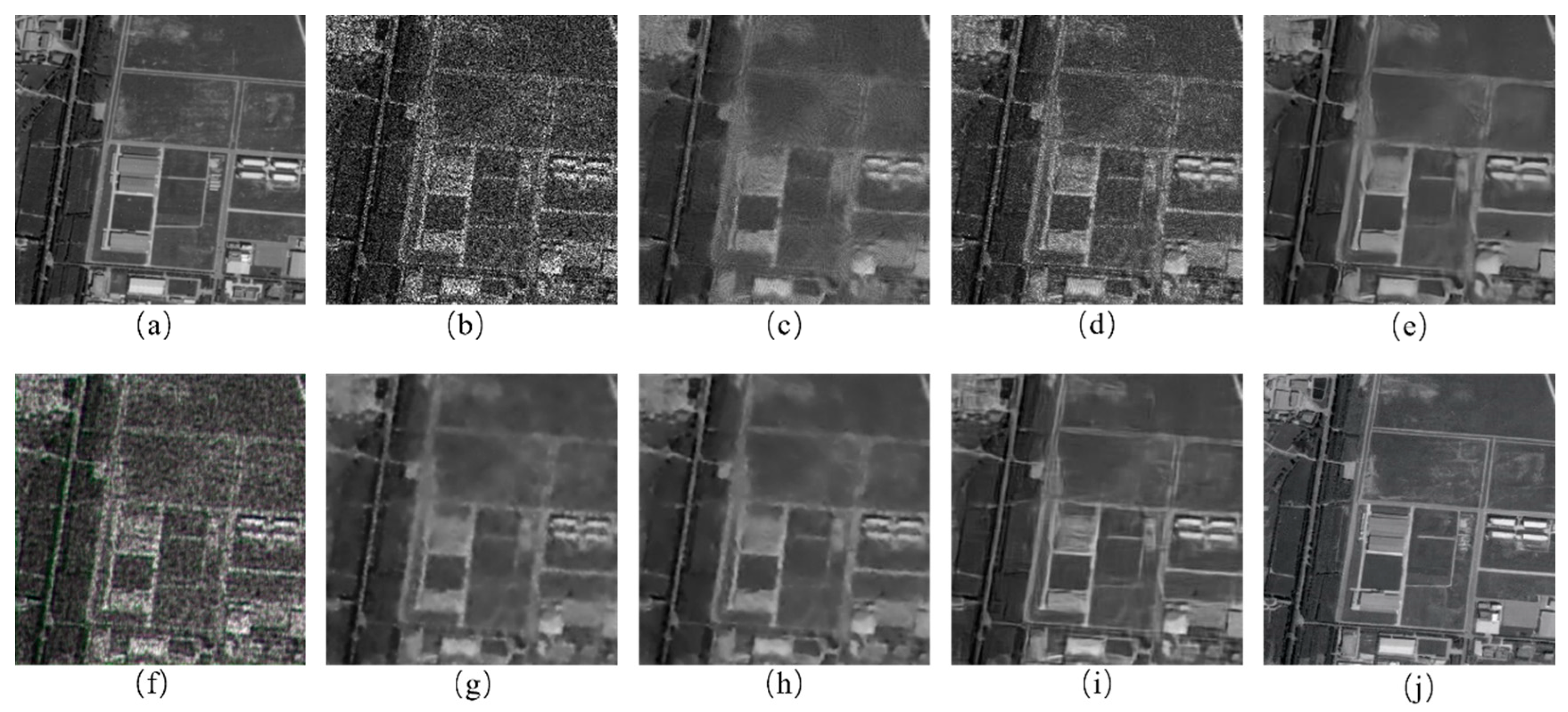
4.3. Comparative Methods

To verify the reliability and effectiveness of the proposed method, we compared it with seven other well-known SAR image denoising methods, including PPB, SARBM3D SARCNN, SARDRN, SAR Transformer, SAR-ON [42], and SAR-CAM. All the methods have been trained with the same datasets mentioned before, the same as our method. We conducted evaluations using both simulated image datasets and real-world image data. The evaluation was carried out using both subjective observation and quantitative indicators.

4.4. Synthetic Image Analysis

The quantitative indicators used in this experiment were PSNR and SSIM. PSNR is commonly used to measure the quality of denoised images, with higher values indicating better noise suppression. SSIM measures the similarity between two images, assessing denoised image authenticity. Higher values indicate better preservation of edge information and image details. The calculated average PSNR and SSIM values for the four datasets are listed in

Table 1. Averge PSNR values of the simulated datasets, with the best result highlighted in bold.

Datasets	L	PPB	SAR-BM3D	SAR-CNN	SAR-DRN	SAR-Transformer	SAR-ON	SAR-CAM	Proposed
Set12	1	24.84	25.24	25.75	25.64	25.53	25.87	26.34	26.86
	2	25.65	26.78	27.15	26.11	27.22	27.46	27.76	28.04
	4	27.32	28.14	28.55	27.84	28.12	29.01	28.92	29.90
	8	28.19	29.77	29.96	29.13	29.78	29.94	30.49	31.62
	10	28.49	30.23	30.46	29.64	30.39	30.72	31.08	32.04
Classic5	1	23.81	25.78	25.99	25.88	25.50	26.25	27.30	27.86
	2	24.87	26.78	26.87	26.11	27.22	27.46	27.56	28.04
	4	26.04	28.14	28.22	27.84	28.12	29.01	28.99	29.90
	8	27.13	29.77	29.74	29.13	29.78	29.94	30.38	31.62
	10	28.01	30.23	30.29	29.64	30.39	30.72	31.26	32.04
McMaster	1	24.97	25.56	25.52	25.82	26.68	26.09	27.80	28.12
	2	26.51	27.34	27.15	27.22	28.82	27.93	29.58	29.83
	4	27.09	29.01	28.96	29.14	29.35	29.01	31.36	31.54
	8	27.82	30.28	30.03	30.56	31.34	30.84	32.67	32.99
	10	29.34	31.42	31.27	31.39	31.72	31.59	33.55	33.73
Kodak24	1	23.52	24.63	24.79	24.57	24.87	24.73	25.04	26.56
	2	24.77	26.12	26.25	25.93	26.33	26.12	27.08	27.93
	4	25.58	28.59	28.80	27.24	28.78	28.69	29.13	29.72
	8	26.64	29.14	30.64	29.33	30.51	29.98	30.26	31.23
	10	27.35	30.03	30.82	30.18	30.78	30.57	31.15	32.07

and

Table 2. Averge SSIM values of the simulated datasets, with the best result highlighted in bold.

Datasets	L	PPB	SAR-BM3D	SAR-CNN	SAR-DRN	SAR-Transformer	SAR-ON	SAR-CAM	Proposed
Set12	1	0.64	0.72	0.71	0.66	0.64	0.70	0.73	0.75
	2	0.72	0.76	0.74	0.70	0.69	0.73	0.79	0.80
	4	0.75	0.79	0.76	0.72	0.73	0.73	0.82	0.87
	8	0.80	0.82	0.76	0.74	0.73	0.77	0.87	0.89
	10	0.80	0.82	0.77	0.75	0.76	0.81	0.88	0.91
Classic5	1	0.61	0.72	0.71	0.65	0.67	0.74	0.77	0.79
	2	0.66	0.74	0.75	0.70	0.71	0.77	0.80	0.81
	4	0.69	0.77	0.77	0.72	0.74	0.81	0.82	0.85
	8	0.72	0.83	0.78	0.75	0.78	0.81	0.85	0.88
	10	0.73	0.85	0.80	0.75	0.82	0.85	0.87	0.88
McMaster	1	0.65	0.74	0.70	0.70	0.72	0.77	0.75	0.80
	2	0.70	0.79	0.74	0.75	0.74	0.81	0.80	0.83
	4	0.74	0.82	0.78	0.74	0.78	0.81	0.83	0.87
	8	0.78	0.86	0.78	0.78	0.83	0.85	0.85	0.90
	10	0.81	0.88	0.84	0.82	0.85	0.90	0.88	0.93
Kodak24	1	0.61	0.76	0.69	0.62	0.69	0.75	0.75	0.77
	2	0.65	0.80	0.73	0.67	0.69	0.76	0.80	0.80
	4	0.67	0.82	0.78	0.72	0.75	0.77	0.82	0.82
	8	0.70	0.84	0.80	0.74	0.77	0.83	0.83	0.88
	10	0.72	0.87	0.82	0.74	0.83	0.85	0.86	0.89

, respectively, with the best result highlighted in bold. The average PSNR/SSIM results show that our method outperforms all compared methods, with a PSNR difference of 0.18–1.52 dB and a SSIM difference of 0–0.05 compared to the second best method.

Subjective visual contrast can be observed in Figure 6. From Figure 6d,f, it is evident that there are obvious noise residues on the denoised images of SAR-BM3D and SAR-DRN; from Figure 6c,g,h, it can be seen that PPB, SAR Transformer, and SAR-ON can all effectively suppress noise, but excessive smoothing may also occur, leading to the loss of some image details; Figure 6e,i show that both SAR-CNN and SAR-CAM can effectively suppress speckle, but the loss of details and edge information in the image after denoising leads to deterioration in image quality. On the other hand, we can refer to Figure 6j, which illustrates that the proposed method successfully removes almost all speckle while preserving the overall structure of the image through the global modeling ability of Swin Transformer. Additionally, based on the powerful generation ability of the diffusion model, it can better restore the edge information and texture details of the image, achieving significant advantages in visual effects compared to the other seven methods. The denoised result obtained with our method has an excellent balance between suppression of speckles and achieving realistic visual effects.

4.5. No Reference Evaluation Indicators

To comprehensively evaluate the effectiveness of the proposed method on real-world SAR images, this paper adopts the following non-reference indicators: equivalent number of looks (ENL) [43], mean of image (MoI) [44], mean of ratio (MoR) [45], edge-preservation degree based on the ratio of average (EPD-ROA) [46], M-index [47].

ENL evaluates the denoising effect in selected homogeneous regions by calculating the ratio of the square of the mean to the variance, expressed as:

$$\mathrm{ENL}={\displaystyle \frac{E{[{\widehat{X}}^2]}^2}{\mathrm{Var}({\widehat{X}}^2)}}.$$

(19)

the higher the ENL, the better the noise suppression effect in homogeneous areas.

MoI is obtained by calculating the mean of the original and denoised images in homogeneous regions. It measures the preservation of mean intensity, with a value closer to 1 indicating better denoising effectiveness:

$$MOI={\displaystyle \frac{{\mu }_x}{{\mu }_y}}$$

(20)

where ${\mu }_x$ represents the mean of the original image, and ${\mu }_y$ represents the mean of the denoised image.

MoR represents the preservation of radiation measurement values in denoising results. Unlike MoI, MoR calculates the mean of the proportional image I (i.e., the ratio of the original image to the denoised image), which can be expressed as:

$$MOR={\mu }_I$$

(21)

where ${\mu }_I$ is the mean of the proportional image.

EPD-ROA assesses the algorithm’s ability to retain edge information. It measures the ratio of average preservation based on adjacent pixels in the denoised and original images:

$$\mathrm{EPD}-\mathrm{ROA}={\displaystyle \frac{{\displaystyle \sum _{i=1}^n}|I_{h1}(i)/I_{h2}(i)|}{{\displaystyle \sum _{i=1}^n}|I_{s1}(i)/I_{s2}(i)|}}$$

(22)

$I_{h1}(i)$ and $I_{h2}(i)$ represent two adjacent pixels of the denoised image, while $I_{s1}(i)$ and $I_{s2}(i)$ represent two adjacent pixels of the original image. EPD-ROA-VD and EPD-ROA-HD indicate the EPD-ROA values in the horizontal and vertical directions, respectively.

M-index consists of three coefficient combinations: $r_{\widehat{\mathrm{ENL}}}$, $r_{\mu }$, $\delta h$.

$r_{\widehat{\mathrm{ENL}}}$ can be expressed as comparing n homogeneous regions on noisy and scaled images:

$$r_{\widehat{\mathrm{ENL}}}={\displaystyle \frac{1}{n}}\sum _{i=1}^n{\displaystyle \frac{|{\widehat{\mathrm{ENL}}}_{\mathrm{noisy}}(i)-{\widehat{\mathrm{ENL}}}_{\mathrm{ratio}}(i)|}{{\widehat{\mathrm{ENL}}}_{\mathrm{noisy}}(i)}}$$

(23)

the ideal value of $r_{\widehat{\mathrm{ENL}}}$ should be close to 0.

The equation for calculating the average proportion ${\mu }_N$ of $n$ homogenous regions (the same as the region selected for calculating $r_{\widehat{\mathrm{ENL}}}$) can be expressed as:

$$r_{\mu }={\displaystyle \frac{1}{n}}\sum _{i=1}^n|1-{\mu }_N(i)|$$

(24)

$\delta h$ is based on Haralick homogeneity texture [46], and homogeneity $h_z$ can be expressed as

$$h_z=\sum _i\sum _j{\displaystyle \frac{1}{1+{(i-j)}^2}}\cdot p_z(i,j)$$

(25)

where $p_z(i,j)$ represents the co-occurrence matrix at any position on the scale image $z$. The distance between the homogeneity $h_o$ of ratio image compared with the homogeneity $\delta h$ of the random permuted the ratio image itself, it can be represented as:

$$\delta h={\displaystyle \frac{\mid h_o-h_g\mid }{h_o}}$$

(26)

the closer its value is to 0, the better the denoising effect.

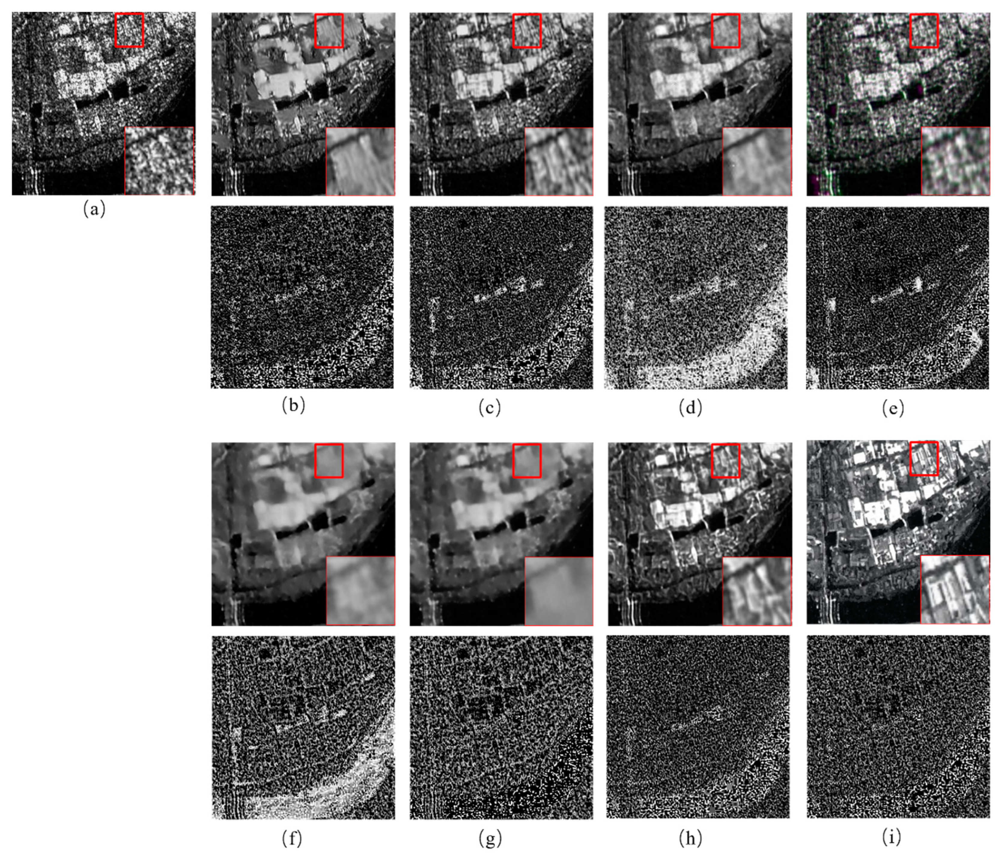
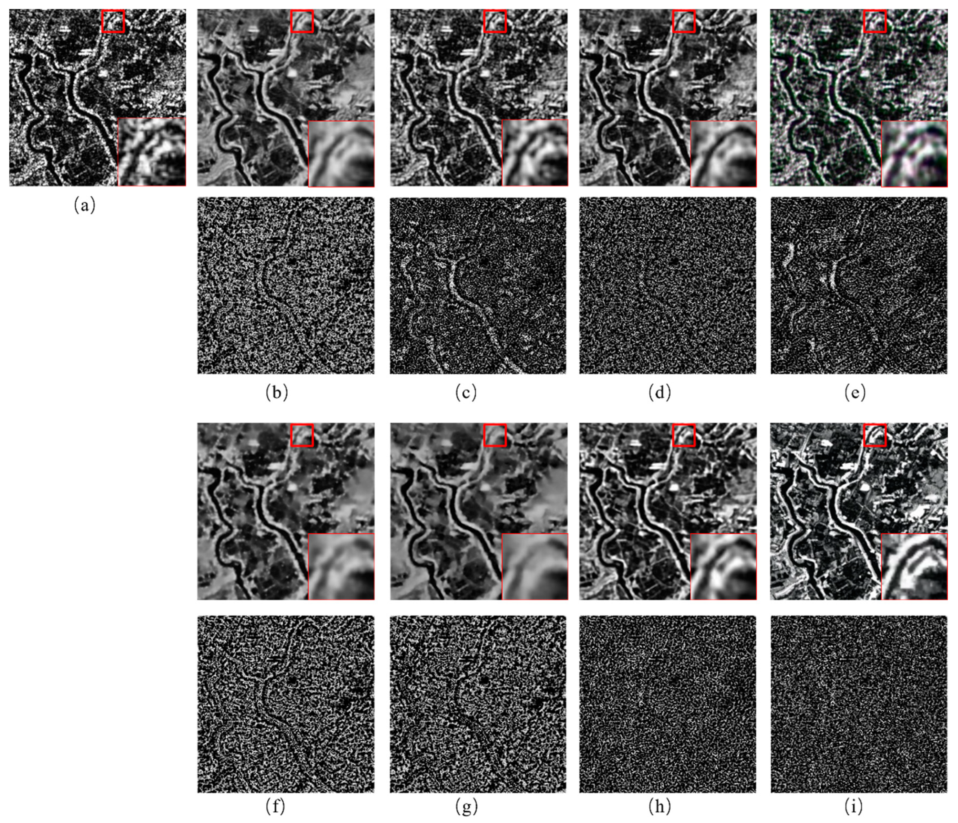
4.6. Real Images Analysis

To further evaluate the effectiveness of the proposed method, SAR images from three different sensors were used and compared with seven other SAR denoising methods. The analysis of the results included subjective evaluation and no reference evaluation indicators. Figure 7b–i displays the results of different denoising methods on SAR1 images. Although PPB, SAR Transformer, and SAR-ON have strong noise suppression effects, they excessively smooth the images, significantly losing edge information and decreasing image quality. SAR-CNN suffers from boundary blurring and artifacts. SAR-BM3D and SAR-DRN can effectively suppress noise and preserve some edge information, but residual noise remains. SAR-CAM has a good balance between suppressing noise and effectively preserving edge information, but it has shortcomings in details. Compared with the above denoising methods, our method not only effectively suppresses noise but also preserves the texture and edge information of the image more completely and obtains more precise details. Meanwhile, the effectiveness of denoising algorithms can be assessed using the ratio image, which is the ratio of the denoised image to the noisy image. The ideal denoising algorithm should result in a ratio image that does not contain visible texture structures, indicating that some essential texture structures have been excessively smoothed out. The ratio image in Figure 7 shows that our method has little geometric structure, suggesting that our method can effectively reduce noise without sacrificing texture. Other methods overly smooth some textures and lose a lot of image details.

Figure 8b–i shows the denoising results and corresponding ratio images of different denoising algorithms on Radarsat2 images. Similar to the results of SAR1, PPB, SAR Transformer, and SAR-ON methods exhibit varying degrees of over-smoothing and artifacts. The noise suppression effect of SAR-BM3D and SAR-DRN is not ideal. SAR-CNN can effectively suppress noise, but residual noise still exists, and there are issues with edge blurring, which decreased image quality in the results. SAR-CAM can effectively suppress noise while preserving the texture and structure of images but has the problem of artifacts and blurred details. In contrast, our method effectively suppresses noise while protecting the edges and details of the image. On the other hand, from the perspective of ratio images, various lines and textures in noisy images can be observed in the scale images of PPB and SAR-BM3D methods. The same problem also occurs in the denoising results of SAR Transformer and SAR-ON methods. Some textures, such as lines and circles, can also be seen in the ratio images of SAR-CNN, SAR-DRN, and SAR-CAM, while our method cannot detect any geometric structure in the ratio image.

The final denoising results of real SAR images are shown in Figure 9b–i. Similar to the previous results, both SAR-CAM and our method outperform other methods in noise suppression and image texture, with our method excelling in preserving image details over SAR-CAM. Turning to the ratio image, it can also be observed that SAR-CAM and our method almost cannot see the texture of noisy images. In contrast, other methods can clearly see the geometric structures, such as curves, in noisy images.

Based on the above subjective comparison and analysis, our method demonstrates effective noise suppression capabilities. In contrast to other methods, it retains more complex textures and edge information while providing more precise image details. This also proves that our method has outstanding advantages in removing noisy images with a large amount of high-frequency information, such as artificial buildings.

In order to comprehensively compare the effectiveness of various methods, we have introduced non-reference indicators as objective evaluation indicators, as shown in

Table 3. Evaluation index of the real dataset, with the best result highlighted in bold and second best result highlighted in red.

Datasets	Method	ENL	MoI	MoR	M-Index	EPD-ROA
						VD	HD
SAR1	PPB	153	0.9239	0.8922	10.813	0.8208	0.8031
	SAR-BM3D	157	0.9268	0.8710	14.458	0.7965	0.7408
	SAR-CNN	167	0.9033	0.8944	14.311	0.8025	0.7417
	SAR-DRN	152	0.9480	0.8978	18.733	0.7802	0.7174
	SAR-Transformer	215	0.8887	0.8427	11.930	0.7765	0.7119
	SAR-ON	171	0.9001	0.8573	11.266	0.7965	0.7298
	SAR-CAM	145	0.8997	0.8796	9.581	0.7832	0.7263
	Proposed	203	0.9484	0.8994	8.438	0.8480	0.8367
SAR2	PPB	577	0.8586	0.8129	24.031	0.7219	0.7155
	SAR-BM3D	287	0.8999	0.8842	28.830	0.7485	0.7384
	SAR-CNN	515	0.9209	0.8704	19.832	0.7417	0.7356
	SAR-DRN	588	0.9331	0.9064	15.761	0.7124	0.7021
	SAR-Transformer	513	0.9349	0.9080	22.620	0.7210	0.7136
	SAR-ON	703	0.9010	0.8697	23.409	0.7211	0.7137
	SAR-CAM	289	0.8582	0.8380	12.076	0.7169	0.7079
	Proposed	937	0.9639	0.9314	10.663	0.7882	0.7924
SAR3	PPB	315	0.8493	0.7579	13.466	0.7599	0.7702
	SAR-BM3D	204	0.9290	0.8938	7.003	0.7966	0.8081
	SAR-CNN	212	0.9305	0.8791	8.863	0.7848	0.7942
	SAR-DRN	186	0.8831	0.9045	4.425	0.7955	0.7970
	SAR-Transformer	316	0.8945	0.8105	14.232	0.7580	0.7753
	SAR-ON	327	0.9147	0.9007	12.146	0.7720	0.7855
	SAR-CAM	291	0.9290	0.9793	7.135	0.7907	0.7912
	Proposed	351	0.9672	0.9872	5.087	0.8799	0.8949

. The best results are highlighted in bold, while the second-best results are highlighted in red. For the denoising results of three different sensor images, we selected 100 regions of interest, calculated accumulative ENL values, and averaged other indicator values of each image dataset. The regions of interest we have selected cover areas that can reflect the effects of all indicators, such as ENL focusing more on homogeneous regions and EPD-ROA focusing more on regions with edge features. Note that no reference evaluation indicators were used for comparing the effects of different methods on the same image. Taking SAR1 and SAR2 as examples, we can see that the ENL value of the denoising results of SAR2 is higher than that of SAR1, while the EPD-ROA value is contrary. In addition to the various statistical characteristics of SAR images, the proportion of homogeneous regions in the scene of SAR2 is significantly higher than that of SAR1, while the edges of SAR1 are more than that of SAR2. Our method obtains the sub-optimal ENL value on SAR1, and the ENL values of SAR2 and SAR3 are optimal, which indicates that our method has a strong ability to suppress speckles. On the other hand, our method is closer to 1 in both MOI and MOR values on all three SAR images, indicating that our method can effectively preserve radiation information. Our method achieved the best EPD-ROA results in both HD and VD, especially for SAR3, where our method outperformed other methods in terms of EPD-ROA values. This indicates that our method has significant advantages in preserving edge information. Finally, for M-index, our results achieved optimal or sub-optimal results on all three images, demonstrating that our method can effectively preserve image details.

In summary, by comparing all non-local and deep learning-based methods with the proposed method through non-reference indicators, it is once again proven that our method can effectively suppress noise while maintaining radiation information. Our method also has excellent results in restoring edge information and image details. Thus, we can conclude that our method delivers outstanding despeckling results across SAR images from different sensors and noise levels.

4.7. Ablation Study

To further demonstrate the effectiveness of the proposed method, we need to conduct an in-depth analysis of the roles of important components in the network structure, such as Swin Transformer Block and PD Refinement, as well as the values of some critical hyperparameters.

4.7.1. SwinTransformer Block Effect

In our method, the primary function of Swin Transformer Blocks is to better extract the global dependencies and local features of SAR images, enabling the algorithm to suppress noise while better preserving the texture and structural information of the image and preventing excessive smoothing. In order to analyze the advantages of Swin Transformer Blocks, we designed four control experiments and used PSNR and SSIM indicators to verify the results, as shown in

Table 4. Control experiments designed for ablation study, where channels in the table represent the final number of channels obtained through downsampling, and checkmarks means with ST Blocks. Checkmarks indicates the presence of ST Blocks and cross marks means without ST Blocks.

Experiment Name	ST Blocks	Channels	Numbers of Res Blocks
Experiment 1	✓	768	2
Experiment 2	✓	768	3
Experiment 3	✓	512	2
Experiment 4	✕	768	2

.

To verify the effectiveness of Swin Transformer Blocks and the stability of the model after their addition, we randomly selected 100 images from the UC Merced land use dataset [48], added noise of L = 1, 2, 4, 8, 10 to the optical images, and calculated the average PSNR and SSIM values. The results are presented in

Table 5. Average PSNR and SSIM results in the ablation experiments, with the best result highlighted in bold.

Experiment Name	L = 1 PSNR (dB)/SSIM	L = 2 PSNR (dB)/SSIM	L = 4 PSNR (dB)/SSIM	L = 8 PSNR (dB)/SSIM	L = 10 PSNR (dB)/SSIM
Experiment 1	26.85/0.80	29.41/0.82	31.00/0.86	32.13/0.87	33.03/0.90
Experiment 2	26.11/0.75	29.23/0.80	29.94/0.85	30.82/0.86	31.79/0.88
Experiment 3	26.38/0.72	29.02/0.79	29.38/0.82	30.46/0.86	31.62/0.85
Experiment 4	23.53/0.72	27.55/0.79	28.79/0.83	29.67/0.85	30.15/0.85

, with the best results highlighted in bold. It is evident that the results after adding ST Blocks are almost always better than before. Despite Experiment 3 having fewer channels than Experiment 4, the results in Experiment 3 are still better than those in Experiment 4 in most cases, proving that DDPM combined with ST Blocks is more conducive to our despeckling tasks. On the other hand, we also found that increasing the number of channels is beneficial for improving the information of our method, whereas increasing the number of ResBlocks did not yield the same improvement. Therefore, the network in our method used 768 channels and 2 ResBlocks.

4.7.2. PD Refinement Effect

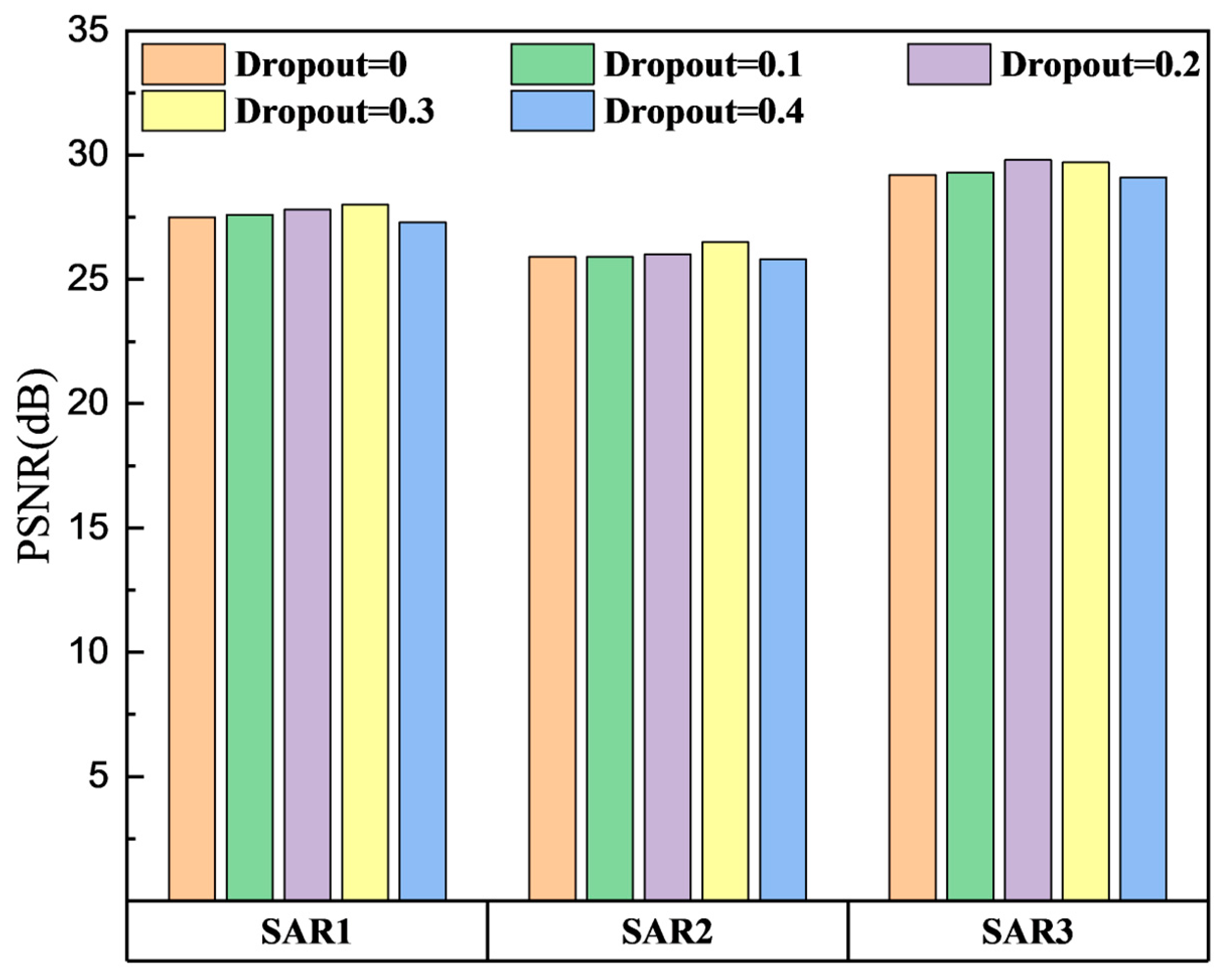
The powerful learning and generation capabilities of DDPM enable us to achieve good results on the training validation set. However, since simulated SAR data were used in the training stages, this inevitably leads to bias when the algorithm despeckles real-world SAR data. In the post-processing stage, we use PD refinement to enhance algorithm stability and make the algorithm more adaptable to real-world SAR data. To verify the effectiveness of PD refinement, we despeckled Sentinel-1 images with and without PD refinement, and the results are shown in Figure 10. We can see that after using the PD Refinement strategy, not only the despeckling results are clearer, but the edge structure is restored better, and the phenomenon of artifacts is greatly eliminated, proving the advantage of using this post-processing strategy for despeckling real-world SAR images.

4.7.3. Dropout Rate

Dropout is a vital part of this method, which can reduce overfitting, enhance model generalization ability, and improve model robustness. Considering the high complexity of our model and the large amount of simulated SAR images used for training, it is necessary to perform a dropout operation. However, dropout randomly removes some neurons, making the neural network more complex and challenging to interpret and understand. Therefore, we need to adjust the dropout rate to grasp the number of deleted neurons so that our model can better adapt to real-world SAR data. Five different dropout rates were used for training and validated on the three real SAR datasets, as shown in Figure 11. It is evident that the dropout operation effectively alleviates the overfitting problem of the model and enhances its stability for the method proposed in this article. When a dropout rate of 0.3 is used, the model’s generalization is strongest. However, when the dropout rate increases to 0.4, the model’s performance begins to decline due to the underfitting problem caused by deleting too many neurons.

4.7.4. Time Analysis

Finally, we also need to explore the time required for training by adding ST Block and PD Refinement to avoid excessive time consumption and a significant cost burden on denoising tasks. We selected images of the same resolution as input, iterated 1000 times, and calculated the average inference time for 100 images. The training time and inference time obtained are shown in

Table 6. Training time and inference time, where inference time means the average inference time for single image.

Method	Training Time	Inference Time
DDPM	4228 s	84 s
Proposed method	4704 s	86 s

. Table 6 indicates that DDPM requires a long training time mainly caused by the sampling stage [49]. After adding ST Block and PD Refinement, the training time, has increased, but it is still within an acceptable range. Therefore, the time consumption issue of the proposed model needs further improvement.

5. Conclusions

In this article, we propose a SAR despeckling algorithm based on the DDPM framework and Swin Transformer. In addition, the PD refinement process was adopted at the post-process stage to adapt the read-SAR images better. Through speckle reduction experiments on simulated SAR images with different noise levels and real-world SAR images obtained from multiple sensors, our method has demonstrated excellent noise suppression effects while preserving more edge information and restoring more image details than other methods. The improvement of the network structure and post-processing measures greatly reduces the instability of the DDPM model when denoising real-world SAR data, and it has good denoising performance for SAR images obtained under different sensors or with various scenes. Moreover, besides achieving superior visual results, our method performs well in quantitative metrics, confirming its effectiveness and robustness in speckle removal tasks. Equally important is that excellent noise suppression ability and visual effects provide a solid foundation for downstream tasks such as SAR target recognition and interpretation.

Nevertheless, the proposed method still has room for improvement. Future efforts should focus on improving the sampling speed of DDPM and making the model more lightweight.

References

1. Moreira, J. Improved Multi Look Techniques Applied to SAR and Scan SAR Imagery. In Proceedings of the International Geoscience and Remote Sensing Symposium IGARSS 90, College Park, MD, USA, 20–24 May 1990. [Google Scholar]
2. Lee, J.S. Digital Image Enhancement and Noise Filtering by Use of Local Statistics. IEEE Trans. Pattern Anal. Mach. Intell. 2009; PAMI-2, 165–168. [Google Scholar]
3. Frost, V.S.; Stiles, J.A.; Shanmugan, K.S.; Holtzman, J.C. A Model for Radar Images and Its Application to Adaptive Digital Filtering of Multiplicative Noise. IEEE Trans. Pattern Anal. Mach. Intell. 1982, 4, 157–166. [Google Scholar] [CrossRef]
4. Kuan, D.T.; Sawchuk, A.A.; Strand, T.C.; Chavel, P. Adaptive Noise Smoothing Filter for Images with Signal-Dependent Noise. IEEE Trans. Pattern Anal. Mach. Intell. 1985, 7, 165–177. [Google Scholar] [CrossRef] [PubMed]
5. Lopes, A.; Nezry, E.; Touzi, R.; Laur, H. Maximum a Posteriori Speckle Filtering and First Order Texture Models in Sar Images. In Proceedings of the International Geoscience & Remote Sensing Symposium, College Park, MD, USA, 20–24 May 1990. [Google Scholar]
6. Guo, H.; Odegard, J.E.; Lang, M.; Gopinath, R.A.; Selesnick, I.W.; Burrus, C.S. Wavelet based speckle reduction with application to SAR based ATD/R. In Proceedings of the Image Processing, Austin, TX, USA, 13–16 November 1994; pp. 75–79. [Google Scholar]
7. Franceschetti, G.; Pascazio, V.; Schirinzi, G. Iterative homomorphic technique for speckle reduction in synthetic-aperture radar imaging. J. Opt. Soc. Am. A 1995, 12, 686–694. [Google Scholar] [CrossRef]
8. Gagnon, L.; Jouan, A. Speckle filtering of SAR images: A comparative study between complex-wavelet-based and standard filters. In Proceedings of the Optical Science, Engineering and Instrumentation ’97, San Diego, CA, USA, 27 July–1 August 1997. [Google Scholar]
9. Chang, S.; Yu, B.; Vetterli, M. Spatially adaptive wavelet thresholding with context modeling for image denoising. IEEE Trans. Image Process. 2000, 9, 1522–1531. [Google Scholar] [CrossRef]
10. Argenti, F.; Alparone, L. Speckle removal from SAR images in the undecimated wavelet domain. IEEE Trans. Geosci. Remote Sens. 2002, 40, 2363–2374. [Google Scholar] [CrossRef]
11. Deledalle, C.A.; Denis, L.; Tupin, F. Iterative weighted maximum likelihood denoising with probabilistic patch-based weights. IEEE Trans Image Process 2009, 18, 2661–2672. [Google Scholar] [CrossRef]
12. Parrilli, S.; Poderico, M.; Angelino, C.V.; Verdoliva, L. A Nonlocal SAR Image Denoising Algorithm Based on LLMMSE Wavelet Shrinkage. IEEE Trans. Geosci. Remote Sens. 2012, 50, 606–616. [Google Scholar] [CrossRef]
13. Deledalle, C.A.; Denis, L.; Tupin, F.; Reigber, A.; Jager, M. NL-SAR: A unified Non-Local framework for resolution-preserving (Pol)(In)SAR denoising. IEEE Trans. Geosci. Remote Sens. 2014, 53, 2021–2038. [Google Scholar] [CrossRef]
14. Cozzolino, D.; Parrilli, S.; Scarpa, G.; Poggi, G. Fast Adaptive Nonlocal SAR Despeckling. IEEE Geoence Remote Sens. Lett. 2013, 11, 524–528. [Google Scholar] [CrossRef]
15. Dong, C.; Loy, C.C.; He, K.; Tang, X. Image Super-Resolution Using Deep Convolutional Networks. IEEE Trans. Pattern Anal. Mach. Intell. 2016, 38, 295–307. [Google Scholar] [CrossRef]
16. Tian, C.; Fei, L.; Zheng, W.; Xu, Y.; Zuo, W.; Lin, C.W. Deep Learning on Image Denoising: An overview. Neural Netw. 2020, 131, 251–275. [Google Scholar] [CrossRef] [PubMed]
17. Chierchia, G.; Cozzolino, D.; Poggi, G.; Verdoliva, L. SAR image despeckling through convolutional neural networks. In Proceedings of the IEEE International Geoscience and Remote Sensing Symposium (IGARSS), Fort Worth, TX, USA, 23–28 July 2017; pp. 5438–5441. [Google Scholar]
18. Wang, P.; Zhang, H.; Patel, V.M. SAR Image Despeckling Using a Convolutional Neural Network. IEEE Signal Process. Lett. 2017, 24, 1763–1767. [Google Scholar] [CrossRef]
19. Vitale, S.; Ferraioli, G.; Pascazio, V. Multi-Objective CNN-Based Algorithm for SAR Despeckling. IEEE Trans. Geosci. Remote Sens. 2021, 59, 9336–9349. [Google Scholar] [CrossRef]
20. Zhang, Q.; Yuan, Q.Q.; Li, J.; Yang, Z.; Ma, X.S. Learning a Dilated Residual Network for SAR Image Despeckling. Remote Sens. 2018, 10, 18. [Google Scholar] [CrossRef]
21. Vaswani, A.; Shazeer, N.M.; Parmar, N.; Uszkoreit, J.; Jones, L.; Gomez, A.N.; Kaiser, L.; Polosukhin, I. Attention is All you Need. In Proceedings of the NIPS’17: Proceedings of the 31st International Conference on Neural Information Processing Systems, Long Beach, CA, USA, 4–9 December 2017. [Google Scholar]
22. Perera, M.V.; Bandara, W.G.C.; Valanarasu, J.M.J.; Patel, V.M. Transformer-Based Sar Image Despeckling. In Proceedings of the IEEE International Geoscience and Remote Sensing Symposium (IGARSS), Kuala Lumpur, Malaysia, 17–22 July 2022; pp. 751–754. [Google Scholar]
23. Ko, J.; Lee, S. SAR Image Despeckling Using Continuous Attention Module. IEEE J. Sel. Top. Appl. Earth Observ. Remote Sens. 2022, 15, 3–19. [Google Scholar] [CrossRef]
24. Goodfellow, I.; Pouget-Abadie, J.; Mirza, M.; Xu, B.; Warde-Farley, D.; Ozair, S.; Courville, A.; Bengio, Y. Generative adversarial networks. Commun. ACM 2020, 63, 139–144. [Google Scholar] [CrossRef]
25. Wang, P.; Zhang, H.; Patel, V.M. Generative adversarial network-based restoration of speckled SAR images. In Proceedings of the 2017 IEEE 7th International Workshop on Computational Advances in Multi-Sensor Adaptive Processing (CAMSAP), Curaçao, The Netherlands, 10–13 December 2017. [Google Scholar]
26. Gu, F.; Zhang, H.; Wang, C. A GAN-based Method for SAR Image Despeckling. In Proceedings of the SAR in Big Data Era: Models, Methods and Applications, Beijing, China, 5–6 August 2019. [Google Scholar]
27. Liu, R.; Li, Y.; Jiao, L. SAR Image Specle Reduction based on a Generative Adversarial Network. In Proceedings of the 2020 International Joint Conference on Neural Networks (IJCNN), Glasgow, UK, 19–24 July 2020. [Google Scholar]
28. Perera, M.V.; Nair, N.G.; Bandara, W.G.C.; Patel, V.M. SAR Despeckling Using a Denoising Diffusion Probabilistic Model. IEEE Geosci. Remote Sens. Lett. 2023, 20, 4005305. [Google Scholar] [CrossRef]
29. Dalsasso, E.; Denis, L.; Tupin, F. SAR2SAR: A semi-supervised despeckling algorithm for SAR images. IEEE J. Sel. Top. Appl. Earth Obs. Remote Sens. 2021, 14, 4321–4329. [Google Scholar] [CrossRef]
30. Ma, X.; Wang, C.; Yin, Z.; Wu, P. SAR Image Despeckling by Noisy Reference-Based Deep Learning Method. IEEE Trans. Geosci. Remote Sens. 2020, 58, 8807–8818. [Google Scholar] [CrossRef]
31. Dalsasso, E.; Denis, L.; Tupin, F. As if by magic: Self-supervised training of deep despeckling networks with MERLIN. IEEE Trans. Geosci. Remote Sens. 2021, 60, 4704713. [Google Scholar] [CrossRef]
32. Molini, A.B.; Valsesia, D.; Fracastoro, G.; Magli, E. Speckle2Void: Deep Self-Supervised SAR Despeckling with Blind-Spot Convolutional Neural Networks. IEEE Trans. Geosci. Remote Sens. 2021, 60, 5204017. [Google Scholar] [CrossRef]
33. Patel, V.M.; Easley, G.R.; Chellappa, R.; Nasrabadi, N.M. Separated Component-Based Restoration of Speckled SAR Images. IEEE Trans. Geosci. Remote Sens. 2014, 52, 1019–1029. [Google Scholar] [CrossRef]
34. Brock, A.; Donahue, J.; Simonyan, K. Large scale GAN training for high fidelity natural image synthesis. arXiv 2018, arXiv:1809.11096. [Google Scholar]
35. Zhang, C.; Yue, P.; Tapete, D.; Jiang, L.; Shangguan, B.; Huang, L.; Liu, G. A deeply supervised image fusion network for change detection in high resolution bi-temporal remote sensing images. ISPRS J. Photogramm. Remote Sens. 2020, 166, 183–200. [Google Scholar] [CrossRef]
36. Zeyde, R.; Elad, M.; Protter, M. On Single Image Scale-Up Using Sparse-Representations. In Curves and Surfaces; Springer: Berlin/Heidelberg, Germany, 2012; pp. 711–730. [Google Scholar]
37. Foi, A.; Katkovnik, V.; Egiazarian, K. Pointwise shape-adaptive DCT for high-quality denoising and deblocking of grayscale and color images. IEEE Trans. Image Process. 2007, 16, 1395–1411. [Google Scholar] [CrossRef] [PubMed]
38. Zhang, L.; Wu, X.; Buades, A.; Li, X. Color demosaicking by local directional interpolation and nonlocal adaptive thresholding. J. Electron. Imaging 2011, 20, 023016. [Google Scholar]
39. Franzen, R. Kodak Lossless True Color Image Suite. Available online: https://www.scirp.org/reference/referencespapers?referenceid=727938 (accessed on 18 July 2024).
40. Kingma, D.P.; Ba, J. Adam: A Method for Stochastic Optimization. arXiv 2014, arXiv:1412.6980. [Google Scholar]
41. He, K.; Zhang, X.; Ren, S.; Sun, J. Delving deep into rectifiers: Surpassing human-level performance on imagenet classification. In Proceedings of the IEEE International Conference on Computer Vision, Las Condes, Chile, 11–18 December 2015; pp. 1026–1034. [Google Scholar]
42. Perera, M.V.; Bandara, W.G.C.; Valanarasu, J.M.J.; Patel, V.M. SAR Despeckling Using Overcomplete Convolutional Networks. In Proceedings of the IEEE International Geoscience and Remote Sensing Symposium (IGARSS), Kuala Lumpur, Malaysia, 17–22 July 2022; pp. 401–404. [Google Scholar]
43. Dellepiane, S.G.; Angiati, E. Quality Assessment of Despeckled SAR Images. IEEE J. Sel. Top. Appl. Earth Observ. Remote Sens. 2014, 7, 691–707. [Google Scholar] [CrossRef]
44. Di Martino, G.; Poderico, M.; Poggi, G.; Riccio, D.; Verdoliva, L. Benchmarking Framework for SAR Despeckling. IEEE Trans. Geosci. Remote Sens. 2014, 52, 1596–1615. [Google Scholar] [CrossRef]
45. Ma, X.S.; Shen, H.F.; Zhao, X.L.; Zhang, L.P. SAR Image Despeckling by the Use of Variational Methods With Adaptive Nonlocal Functionals. IEEE Trans. Geosci. Remote Sens. 2016, 54, 3421–3435. [Google Scholar] [CrossRef]
46. Haralick, R.M.; Shanmugam, K.; Dinstein, I. Textural Features for Image Classification. IEEE Trans. Syst. Man Cybern. 1973; SMC-3, 610–621. [Google Scholar] [CrossRef]
47. Gomez, L.; Ospina, R.; Frery, A.C. Unassisted Quantitative Evaluation of Despeckling Filters. Remote Sens. 2017, 9, 23. [Google Scholar] [CrossRef]
48. Yang, Y.; Newsam, S. Bag-of-visual-words and spatial extensions for land-use classification. In Proceedings of the ACM SIGSPATIAL International Workshop on Advances in Geographic Information Systems, San Jose, CA, USA, 2–5 November 2010. [Google Scholar]
49. Dhariwal, P.; Nichol, A. Diffusion Models Beat GANs on Image Synthesis. In Proceedings of the NIPS’21: Proceedings of the 35th International Conference on Neural Information Processing Systems, Virtual, 6–14 December 2021. [Google Scholar]
Figure 1. Overview of forward and reverse processes in diffusion model.
Remotesensing 16 03222 g001
Figure 2. The training and inference framework in our method. During the training phase, we will use the proposed DDPM. In the inference stage, we use pre-trained networks and pixel-shuffle down-sampling refinement process to obtain prediction results.
Remotesensing 16 03222 g002
Figure 3. Swin Transformer block, LN means layer norm, MLP means multilayer perceptron.
Remotesensing 16 03222 g003
Figure 4. PD Refinement strategy with stride = 2.
Remotesensing 16 03222 g004
Figure 5. Real SAR images. (a) SAR1. (b) SAR2. (c) SAR3.
Remotesensing 16 03222 g005
Figure 6. Denoised results of different methods for image with L = 1 speckle noise. (a) Original. (b) Noise. (c) PPB. (d) SAR-BM3D. (e) SAR-CNN. (f) SAR-DRNt. (g) SAR-Transformer. (h) SAR-ON. (i) SAR-CAM. (j) Proposed.
Remotesensing 16 03222 g006
Figure 7. Results for SAR1 image with ratio image. (a) Noisy image. (b) PPB. (c) SAR-BM3D. (d) SAR-CNN. (e) SAR-DRN. (f) SAR-Transformer. (g) SAR-ON. (h) SAR-CAM. (i) Proposed.
Remotesensing 16 03222 g007
Figure 8. Results for SAR2 image with ratio image. (a) Noisy image. (b) PPB. (c) SAR-BM3D. (d) SAR-CNN (e) SAR-DRN. (f) SAR-Transformer. (g) SAR-ON. (h) SAR-CAM. (i) Proposed.
Remotesensing 16 03222 g008
Figure 9. Results for SAR3 image with ratio image. (a) Noisy image. (b) PPB. (c) SAR-BM3D. (d) SAR-CNN. (e) SAR-DRN. (f) SAR-Transformer. (g) SAR-ON. (h) SAR-CAM. (i) Proposed.
Remotesensing 16 03222 g009
Figure 10. Denoising results. (a) The noise image (b) is denoised using our method without PD refinement, and (c) is denoised using our method with PD refinement.
Remotesensing 16 03222 g010
Figure 11. The average PSNR value of the denoising results of the model on three real SAR datasets under different dropout rates.
Remotesensing 16 03222 g011