InSAR-Driven Dynamic Landslide Hazard Mapping in Highly Vegetated Area

Abstract

Landslide hazard mapping is important to urban construction and landslide risk management. Dynamic landslide hazard mapping considers landslide deformation with changes in the environment. It can show more details of the landslide process state. Landslides in highly vegetated areas are difficult to observe directly, which makes landslide hazard mapping much more challenging. The application of multi-InSAR opens new ideas for dynamic landslide hazard mapping. Specifically, landslide susceptibility mapping reflects the spatial probability of landslides. For rainfall-induced landslides, the scale exceedance probability reflects the temporal probability. Based on the coupling of them, dynamic landslide hazard mapping further considers the landslide deformation intensity at different times. Zigui, a highly vegetation-covered area, was taken as the study area. The landslide displacement monitoring effect of different band SAR datasets (ALOS-2, Sentinel-1A) and different interpretation methods (D-InSAR, PS-InSAR, SBAS-InSAR) were studied to explore a combined application method. The deformation interpreted by SBAS-InSAR was taken as the main part, PS-InSAR data were used in towns and villages, and D-InSAR was used for the rest. Based on the preliminary evaluation and the displacement interpreted by fusion InSAR, the dynamic landslide hazard mappings of the study area from 2019 to 2021 were finished. Compared with the preliminary evaluation, the dynamic mapping approach was more focused and accurate in predicting the deformation of landslides. The false positives in very-high-hazard zones were reduced by 97.8%, 60.4%, and 89.3%. Dynamic landslide hazard mapping can summarize the development of and change in landslides very well, especially in highly vegetated areas. Additionally, it can provide trend prediction for landslide early warning and provide a reference for landslide risk management.

1. Introduction

Landslides are common natural disasters that cause thousands of casualties and huge property losses every year [1]. Preventing and reducing landslide risk effectively is challenging work [2]. Landslide hazard mapping (LHM), which provides a reference for urban planning, is essential for building site selection and emergency evacuation [3].

LHM is a comprehensive evaluation of the spatial probability, temporal probability, and scale probability of landslides based on susceptibility assessment [4]. Early on, there was no unified terminology for LHM, and there were many discussions on the content of evaluation. Then, LHM was further developed in the direction of quantification and systematization [5,6]. Glade et al. [7] and Fell et al. [8] established a landslide risk framework and clarified the concept and process of LHM. The spatial probability of landslides is described by susceptibility assessment based on landslide events [9]. The temporal probability of landslides is analyzed by physical models [10] or statistical models [11,12]. LHM is usually combined with GIS and has been rapidly developed and applied worldwide [13,14].

However, the evolution of landslides is a dynamic process [15]. At different times, due to changes in triggers, such as rainfall [16], earthquakes [17], and reservoir water level fluctuations [18], landslide hazards also change accordingly. Generally, this is positively correlated to rainfall, the earthquake magnitude, and the magnitude and speed of the water level changes. Static LHM cannot reflect such changes. Therefore, dynamic triggers are introduced to characterize the changes in landslide hazards. Guzzetti et al. [19] and Lee et al. [20] calculated the landslide hazard under different extreme rainfalls through the rainfall return period. Kirschbaum et al. [21] and Gariano et al. [22] used dynamic rainfall in different periods as an evaluation factor to carry out dynamic LHM.

The landslide deformation velocity can also be used directly as a time probability factor for dynamic LHM. InSAR has good regional deformation recognition capabilities and can monitor the deformation state of regional landslides in real time [23]. It can provide deformation for dynamic LHM and has been widely used [24,25]. Synthetic aperture radar (SAR) is an all-weather active sensor. Interferometric SAR (InSAR) can implement the high-precision observation of the surface [26]. D-InSAR [27], PS-InSAR [28], and SBAS-InSAR [29] have been widely used in surface deformation detection and landslide monitoring [30,31,32,33,34].

In areas with high vegetation, different radar datasets and solution methods greatly differ in their accuracy of deformation interpretation. Although SAR is a remote sensing radar, it is not affected by weather or light [35]. However, the absorption of radar waves by plant leaves will affect the accuracy of interpretation. Liang et al. [36] and Zhang et al. [37] explored the identification and monitoring of landslides in areas with different densities of vegetation coverage using radar remote sensing in various bands, which shows the anti-interference ability of the C band to vegetation coverage. Walker et al. [38], Oveisgharan et al. [39], and Maghsoudi et al. [40] studied the detection of the terrain, vegetation canopy, and deformation in forest areas using different InSAR interpretation methods. A large number of landslide identification and monitoring studies have shown that landslide deformation monitoring in areas with high vegetation coverage is still quite challenging. Many mountainous areas have lush vegetation and are also prone to landslides. An important task in landslide monitoring and early warning in these areas is to identify surface deformation. This study explores the applicability of different SAR data sources and different interpretation methods in such areas and how to obtain the best possible identification results.

Zigui, a county in the Three Gorges Reservoir Area, was chosen as the study area for dynamic LHM. It has hundreds of landslides and is covered by forest. A preliminary LHM was obtained through landslide susceptibility mapping (LSM) and rainfall return period analysis. A multi-InSAR interpretation method was explored and summarized to calculate the landslide deformation velocity. It was coupled with the preliminary LHM. The dynamic LHM considering landslide deformation provides a more accurate and practical reference for landslide management and provides trend prediction for landslide early warning.

2. Methods

Landslide hazard refers to the possibility of landslides occurring on a certain scale in a certain area within a certain period. It can be evaluated by analyzing the probability of occurrence.

According to the risk framework [7,41], the spatial probability of a landslide is based on susceptibility mapping. In the study area, rainfall is the main factor leading to landslides. The rainfall data are statistically used to calculate the extreme rainfall that can trigger a landslide of a specific scale. The extreme rainfall return period is analyzed to obtain the time probability of landslides. The evaluation formula of a regional landslide hazard ($H$) is as follows:

$$H=P\left(S\right)\times P\left(N_L\right)$$

(1)

where $P\left(S\right)$ is the landslide spatial probability, and $P\left(N_L\right)$ is the landslide time probability.

The evolution of landslides is a dynamic process. The risk will also change at different periods due to changes in triggers. The dynamic assessment of landslide hazards needs to capture the impact of these changes on landslides. InSAR can monitor the regional landslide deformation and provide the deformation data ($D$) for dynamic LHM. The improved formula is as follows:

$$H=P\left(S\right)\times P\left(N_L\right)\times D$$

(2)

The workflow of dynamic LHM includes four steps, as shown in Figure 1. (1) Based on remote sensing identification, field investigation, and landslide cataloging, analyze the landslide characteristics and triggering factors. The spatial probability of landslides is calculated through LSM. (2) Analyze the landslide time probability in different rainfall return periods. Define the scenarios and calculate the preliminary landslide hazard. (3) Calculate the surface deformation velocity in areas with high vegetation coverage by multi-InSAR. (4) According to Equation (2), construct a hazard dynamic evaluation matrix considering the landslide deformation to carry out dynamic LHM.

2.1. Landslide Hazard Mapping

2.1.1. Landslide Spatial Probability Based on LSM

LSM is an intuitive expression of the spatial probability of landslides. Its essence is to use Engineering Geological Analogies (EGAs) to infer the landslide probability based on landslides that have already occurred. LSM methods are divided into three categories: heuristic models, statistical models, and physical models [42,43]. Random forest (RF) was used for the LSM in this study. RF is a commonly used statistical method with good accuracy and generalization abilities [44]. It takes the decision tree model as the basic unit. A “forest” supervised learning algorithm is obtained by integrating many unrelated decision tree models. The result is obtained by calculating the average or voting. During the decision tree building process, features that reduce information uncertainty most are selected to divide the dataset [45]. The evaluation criteria for decision tree node splitting generally include the Information Gain Ratio (IGR) [46] and the Gini Index [47]. To carry out LSM, the regional landslide characteristics need to be analyzed. The factors for landslide susceptibility evaluation can be chosen according to the landslide characteristics, including the geology, topography, hydrology, etc. The landslide data and evaluation factors data are unified and standardized. Landslide points and non-landslide points are randomly selected as positive and negative samples for model training. The model training accuracy is evaluated and debugged to achieve the expected accuracy. The optimized model is used to predict the landslide susceptibility probability in the entire study area. The susceptibility probability is classified, and LSM can be obtained by GIS visualization.

2.1.2. Landslide Time Probability and Preliminary LHM

The landslide time probability can be calculated by its scale exceedance probability. For landslides with detailed records, it is assumed that the time of landslide occurrence follows a Poisson distribution. The time probability ($P\left(N_L\right)$) of at least a landslide in each evaluation unit within a certain recurrence period, such as 5 years, 10 years, 20 years, or 50 years, can be calculated. For rainfall-induced landslides, the Gumbel Model [48] can be used to solve the exceedance probability ($P\left(N_L\right)$) of landslides under specific extreme rainfall conditions, such as 5-year, 10-year, 20-year, and 50-year rainstorm conditions. The preliminary LHM can be calculated according to Equation (1) and divided into four levels (H4: very high hazard; H3: high hazard; H2: moderate hazard; H1: low hazard) according to the local standard [49].

2.2. Multi-InSAR Displacement Detection

Synthetic aperture radar (SAR) moves a small-aperture antenna in a direction. The data obtained at different locations are comprehensively processed to form an equivalent large-aperture radar, thereby improving the azimuth resolution and detection accuracy [50].

InSAR uses two SAR images of the same area to obtain the phase information of each pixel through interference processing. Thus, the positional relationship between ground objects and satellites can be obtained. Differential interferometry InSAR (D-InSAR) removes the terrain phase (${\phi }_t$), atmospheric phase (${\phi }_a$), and noise phase (${\phi }_n$) from the initial interference phase ($\phi$) to obtain the information phase (${\phi }_d$) (Equation (3)):

$$\phi ={\phi }_d+{\phi }_t+{\phi }_f+{\phi }_a+{\phi }_n$$

(3)

PS-InSAR takes N + 1 SAR images covering the same area, selects one of them as the main image, and registers the rest of them to this image to generate a time series differential interferogram. The points that maintain high coherence will be selected to establish and solve the deformation inversion model. It can effectively separate other error phase components and obtain the rate of surface deformation.

Unlike PS-InSAR, SBAS-InSAR takes the time baseline and space baseline as a condition, with less than a certain threshold, and all data are combined by interference pairs. For the No. $j$ scene differential interference pattern ($T_b>T_a$) generated from image $T_a$ and main image $T_b$, after spatial unwrapping, the interference phase ($\delta {\phi }_j$) at any point can be expressed as follows:

$$\delta {\phi }_j={\phi }_{T_b}-{\phi }_{T_a}\approx {\displaystyle \frac{4\pi }{\lambda }}\left(d_{T_b}-d_{T_a}\right)$$

(4)

where ${\phi }_{T_a}$ and ${\phi }_{T_b}$ are the phase differences at $T_a$ and $T_b$, respectively. $j\in [1,\cdots ,N]$. $d_{T_b}$ and $d_{T_a}$ are the accumulated deformation amounts in the line-of-sight direction at $T_a$ and $T_b$ time relative to the initial time ($d_{T_0}=0$), respectively.

Assuming that the deformation in the time interval between $T_a$ and $T_b$ is linear, the surface deformation is piecewise linear during the entire period, and then the deformation phase value of the No. $j$ scene interference pattern is as follows:

$$\delta {\phi }_j={\sum }_{k=T_{a,j}+1}^{T_{b,j}}(T_k-T_{k-1})v_k$$

(5)

The integral of the speed in each period is superimposed over the time interval of the master–slave image. All unwrapped differential interference phases are combined into a matrix:

$$\delta \phi =\mathit{B}\mathit{v}$$

(6)

$\mathit{B}\mathit{v}$ is an M × N matrix. The generalized inverse matrix of $\mathit{B}$ can be obtained through the singular value decomposition method. The final deformation rate or cumulative displacement can be calculated.

2.3. Dynamic LHM Based on Slope Deformation

Based on the preliminary LHM, the dynamic LHM is calculated through the landslide deformation velocity. Rainfall is one of the main factors inducing landslides. Surface deformation is a direct manifestation of landslide failure. LHM based on the rainfall return period assumes that rainfall has the same impact on landslides, and InSAR monitoring results represent the status of landslides. Introducing the deformation into hazard assessment can correct errors and improve the accuracy and timeliness of evaluation results. The deformation obtained by multi-InSAR is divided into four levels according to the velocity and reginal deformation characteristics [51,52]: fast (V4), moderate (V3), slow (V2), and very slow (V1). The velocity classification standard is determined according to the maximum deformation velocity in the study area. The preliminary LHM is superimposed with the slope deformation level to establish a dynamic LHM matrix [53], as shown in

Table 1. Dynamic LHM matrix.

	V4	V3	V2	V1
H4	VHH	VHH	HH	MH
H3	VHH	HH	MH	MH
H2	VHH	HH	MH	LH
H1	HH	MH	LH	LH

VHH: very high hazard (red); HH: high hazard (orange); MH: moderate hazard (yellow); LH: low hazard (green).

.

3. Database

3.1. Geological Background of Zigui

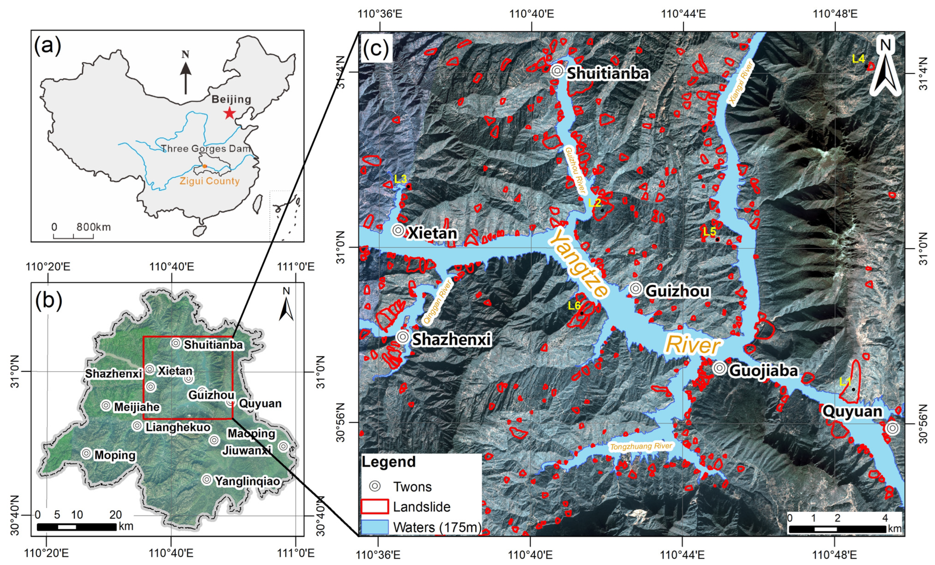
Zigui is in central China, with an area of 485.5 km², and it is 30 km away from the Three Gorges Dam (Figure 2). It has a subtropical continental monsoon climate, with an average annual rainfall of 1336.1 mm. The Yangtze River traverses 64 km of the county. It has 135 first-level tributaries, forming a complex and tortuous reservoir bank.

Zigui belongs to the folded mountains of western Hubei, with an average altitude of over 800 m. It has towering peaks, deep valleys, and a relative height difference of 500 m–1300 m. The terrain slope in the area changes greatly. The Yangtze River gorge area and the transition zone often form steep cliffs. The strata exposure from the Proterozoic to the Quaternary. They spread from old to young, from east to west. They are mainly constructed of terrigenous clastic rocks and carbonate rocks. Magmatic rocks are distributed in the east, and the lithology is mainly neutral and acidic rocks.

Zigui is located at the composite site of the northern end of the Hubei uplift belt of the Neocathaysian tectonic system and the Huaiyang Mountain-shaped tectonic system, which has complex structures. The N-W trending structures developed in the Pre-Sinian metamorphic rock series are composed of several folds and faults accompanied by magmatic activity. The W-E trending structures are distributed in the south and are dominated by folds composed of sedimentary cover. The tectonic of Zigui is stable. Since the Cenozoic, there have been intermittent uplifts and local faulting activities. These faults produced differential activities in the Quaternary, which promoted landslides.

3.2. Dataset

Sentinel-1 and ALOS-2 radar remote sensing datasets were collected for this study. Sentinel-1 carries a C-band synthetic aperture radar with a wavelength of 5.5 cm and a resolution of 5 m × 20 m. A total of 81 scenes of Sentinel-1A ascending orbit data from January 2019 to December 2021 were used to carry out PS-InSAR and SBAS-InSAR monitoring. ALOS-2 was launched on 24 May 2014 and is equipped with the PALSAR-2 sensor. The operating band is the L-band with a wavelength of 25 cm and a resolution of 10 m × 10 m. A total of two scenes of ascending orbit data from 20 May 2019 and 15 July 2019 were obtained for D-InSAR. According to the characteristics of electromagnetic waves, the L-band ALOS-2 image with a longer wavelength has better penetration into vegetation. This gives it a unique advantage in areas with high vegetation coverage. The Copernicus DEM GLO-30 (https://doi.org/10.5270/ESA-c5d3d65, accessed on 28 August 2024), archived on 8 April 2021, was collected. Since the Three Gorge Reservoir Area has been impounded since 2003 and was first impounded to 175 m in 2010, the DEM after 2011 is more suitable for this study. Dataset information is shown in

Table 2. Dataset information.

Type	Name	Resolution/m	Phase	Coverage
SAR	ALOS-2	10	20 May 2019, 15 July 2019	2 scenes, covering 485.5 km2
	Sentinel-1A	5 × 20	1 January 2019~ 28 December 2021	81 scenes, covering 485.5 km2
DEM	COP GLO-30	30	2011~2015	Covering 485.5 km2

. All images fully cover the study area.

3.3. Landslide Inventory

Based on historical landslide data and field investigation, a total of 413 landslides were confirmed in the study area. A detailed landslide inventory recorded the types, time of failure, location, deformation, elements at risk, and other information. The locations and boundaries of these landslides are marked in Figure 1. Most of these landslides were accumulation landslides. They are elongated, tongue-shaped, or semicircular. A total of 104 of them had a volume of more than 10⁶ m³. The largest one was the Xintan landslide (L1 in Figure 2), with a volume of 3 × 10⁷ m³, destroyed on 12 June 1985. A total of 28 landslides were unstable, with a total volume of 7.32 × 10⁷ m³. Most landslides are distributed along the reservoir bank and are closely related to rainfall and reservoir level changes. A total of 198 are on high-steep slopes far from the fluctuation zone. The high vegetation in the study area brings challenges to landslide deformation detection.

4. Results

4.1. LSM in Zigui

The joint action of the geological environment and external triggers causes landslides. The former includes topography, lithology, structures, etc. The latter includes the hydrological environment and others. According to the survey results, the following 12 factors were extracted as indicators for the LSM of the study area: Elevation, Slope, Aspect, Terrain Roughness Index (TRI), Curvature, Plane Curvature, Section Curvature, Lithology, Distance to Fault, Topographic Wetness Index (TWI), Stream Power Index (SPI), and Distance to River. These factors are shown in Figure 3. After collinearity analysis and information gain calculation, the Curvature, TWI, and SPI factors were eliminated, and the remaining nine indicators were used for LSM.

The information value of each factor on the occurrence of landslides was calculated, and the IGR was further calculated, as shown in Figure 4. The IGR reflected the contribution of the factor to the LSM. The factor with the highest IGR was Elevation, reaching 0.0172. The lowest one was the SPI, which is slightly higher than 0.0001. To screen important evaluation factors and improve the accuracy of the LSM, the factors with the lowest IGRs were eliminated to verify the model accuracy. If all factors were retained, the model accuracy was 0.868. The model accuracy was improved to 0.872 when the SPI was eliminated. The model accuracy was further improved to 0.875 when the SPI and Curvature were eliminated. When the SPI, Curvature, and TWI were eliminated, the model accuracy was improved to 0.877, which was the highest among all six models. If we continue to eliminate the Plane Curvature and Profile Curvature, the model accuracy decreases instead. Therefore, the best model is to eliminate the three SPI, TWI, and Curvature factors and retain the remaining nine factors, as shown in

Table 3. LSM modeling accuracy statistics table.

Elimination Factors	RF Model Accuracy
None	0.868
SPI	0.872
SPI, Curvature	0.875
SPI, Curvature, TWI	0.877
SPI, Curvature, TWI, Plane Curvature	0.873
SPI, Curvature, TWI, Plane Curvature, Profile Curvature	0.872

.

All evaluation factors and landslide datasets were resampled to a grid resolution of 25 m × 25 m. Grids without landslides were defined as non-landslide grids. There were 27,785 grids of landslides in the study area. A total of 27,785 non-landslide grids were randomly selected. They were combined with all 27,785 landslide grids to form training samples and verification data. The RF model was constructed in SPSS Pro. The training sample and validation data size ratio was 1:1. All factors were standardized by Z-Score. The optimal hyperparameters of the RF in this study were as follows: bootstrp: true; oob_score: no; max_features: auto; max_depth: 100; min_sanples_leaf: 1; min_samples_split: 2; max_leaf_nodes: 10; min_impurity_decrease: 0; criterion: Gini; min_sample_leaf: 0.

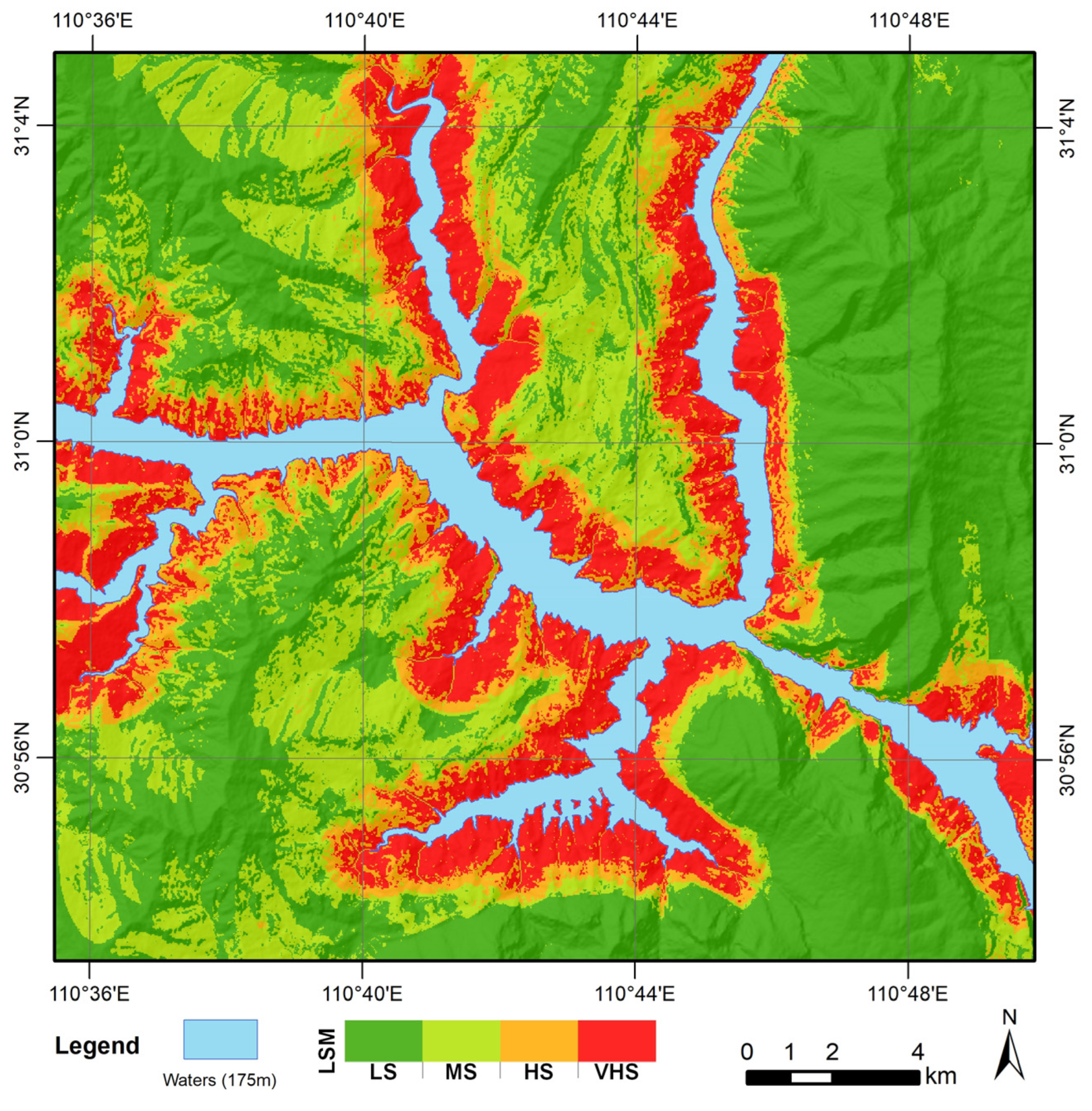
The study area was divided into low-susceptibility (LS) zones, moderate-susceptibility (MS) zones, high-susceptibility (HS) zones, and very-high-susceptibility (VHS) zones. They were divided according to the probability of landslides as [0, 0.4), [0.4, 0.6), [0.6, 0.8), and [0.8, 1] [45], as shown in Figure 5. The VHS zones were distributed along both banks of the Yangtze River trunk and tributaries, while the MS and LS zones were mainly in high-altitude areas and far away from the river. ROC analysis was used for the accuracy evaluation [54], with AUC = 0.877. The frequency ratio method was used to analyze the prediction accuracy, as shown in

Table 4. Frequency ratio analysis of LSM.

Landslide Susceptibility Level	LS	MS	HS	VHS
Landslide grids	1123	4256	4181	18,225
Zone grids	333,901	148,659	83,469	131,069
Landslide percentage	4.04%	15.32%	15.05%	65.59%
Zone percentage	47.90%	21.33%	11.97%	18.80%
Frequency ratio	0.084	0.718	1.257	3.489

. In the LS zones, the frequency ratio was 0.084. In the HS zones, the frequency ratio was 1.257, reaching 3.489 in the VHS zones. The landslide frequency ratio increased significantly with increasing susceptibility. This showed that the RF performed well in predicting landslides in the study area.

4.2. Scenarios and Preliminary LHM

Statistics on the correlation between landslides and rainfall in the study area show that landslides have the greatest correlation with 3-day rain. Based on the Gumbel distribution model and daily rainfall data from 1980 to 2020, the extreme values of the 3-day rainfall of different return periods in the study area were predicted (

Table 5. Extreme rainfall under different return periods in the study area and scenarios.

Scenarios	A	B	C	D
Return period	5 years	10 years	20 years	50 years
3-day rainfall/mm	147.16	171.15	197.14	223.96
Probability	0.2	0.1	0.05	0.02

).

Landslide information, such as the failure time, rainfall intensity, and duration, was extracted from the landslide inventory. The scale of landslides was calculated by comparing the extreme rainfall in each return period. Then, it was compared with the area of the landslide susceptibility zoning. The spatial probabilities of landslides in different return periods and different susceptibility zoning can be calculated. The preliminary LHM was based on the spatial probability, multiplied by the time probability of the return period. The time probability is the reciprocal of the return period. The spatial probability in different return periods is shown in

Table 6. Preliminary LHM based on rainfall return period.

LSM	Calculated Item	Scenarios
		A	B	C	D
VHS	Zone grids	131,069
	Landslide grids	142	1743	6871	18225
	Spatial probability (%)	0.11	1.33	5.24	13.90
	Preliminary hazard (×10−3)	0.20	1.30	2.60	2.80
HS	Zone grids	83,469
	Landslide grids	47	861	1932	4181
	Spatial probability (%)	0.06	1.03	2.31	5.01
	Preliminary hazard (×10−3)	0.10	1.00	1.20	1.00
MS	Zone grids	148,659
	Landslide grids	18	364	1944	4256
	Spatial probability (%)	0.01	0. 24	1.31	2.86
	Preliminary hazard (×10−3)	0.00	0.20	0.70	0.60
LS	Zone grids	333,901
	Landslide grids	0	547	547	1123
	Spatial probability (%)	0.00	0.16	0.16	0.34
	Preliminary hazard (×10−3)	0.00	0.20	0.10	0.10

.

The probability of extreme rainfall-inducing landslides under each scenario was calculated. It was combined with the LSM to realize the preliminary LHM of the study area (Figure 6). As the rainfall intensity increased, the landslide hazard level increased. The high-hazard zoning in each scenario was distributed within about 1 km on both banks of the Yangtze River trunk and tributaries. Among them, the very-high-hazard zonings were mainly located in the following regions: (1) the Xintan landslide (L1 in Figure 2) and surrounding area in the east of the study area; (2) the middle section of the Xiangxi River; (3) near the Kaziwan landslide (L2 in Figure 2) on the left bank of the Guizhou River; (4) the southeast slope on the left bank of the Qinggan River.

4.3. Slope Deformation in High-Vegetation-Coverage Area

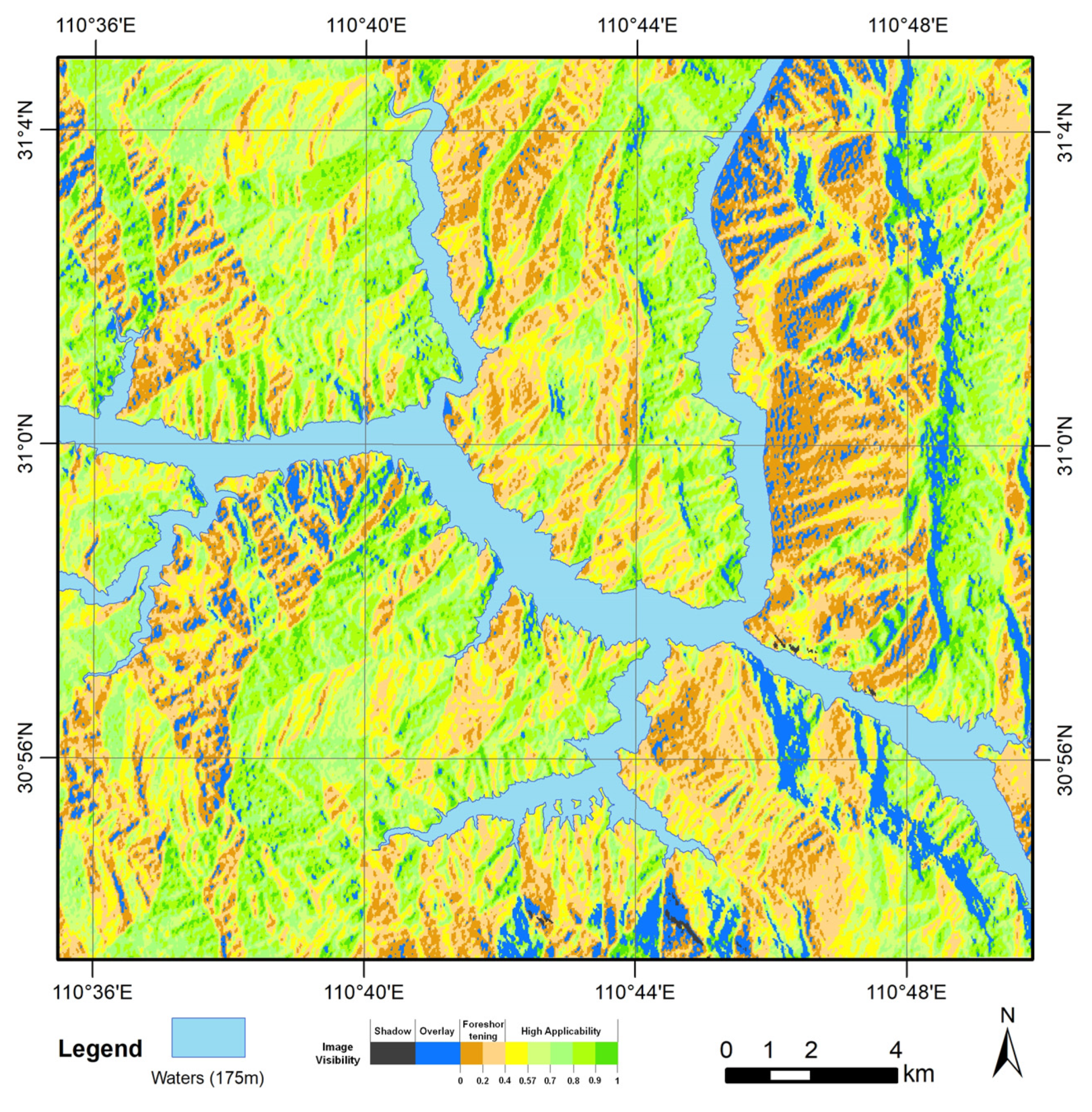
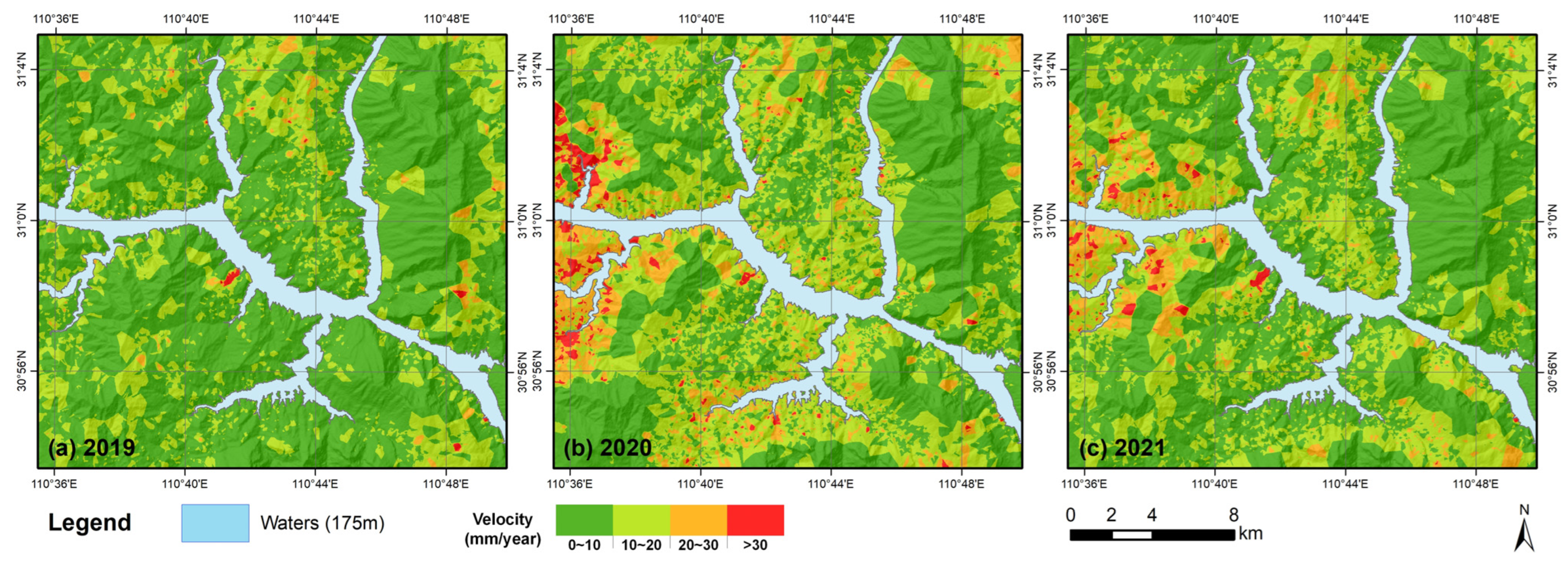
A total of 81 Sentinel-1A ascending orbit images in the study area from 2019 to 2021 were used to interpret the landslide deformation. In 2019, two additional ALOS ascending orbit images were added for D-InSAR interpretation to fill in the gaps in the data, further improving the accuracy of the surface deformation. The visibility of the image sets was 83%, which met the evaluation needs (Figure 7). In this study, a multi-InSAR interpretation fusion method was adopted via SARscape with the high vegetation coverage. The interpretation results of the SBAS-InSAR were taken as the main body, and the PS-InSAR interpretation results were superimposed onto the urban area. The D-InSAR interpretation results were used to supplement the rest of the area in 2019. For the fused deformation map, the Radial Basis Functions were selected for spatial interpolation and divided into four levels [51,52]: V1 (0~10 mm/year), V2 (10~20 mm/year), V3 (20~30 mm/year), and V4 (>30 mm/year). The surface deformation velocity map of the study area was formed with annual time intervals, as shown in Figure 8.

The slope deformation in the study area was negligible in 2019. In 2020, the deformation velocity increased significantly, reaching the highest level in three years. The areas with deformation velocities above 20 mm/year were mainly concentrated in the western and central–southern parts of the study area. In the western part of the study area, the north bank of the Yangtze River is undergoing a highway reconstruction and expansion project, which results in a large deformation variable monitored by InSAR. In 2021, the areas with large slope deformations were the western regions in the study area; the deformations were smaller in 2020. According to the field verification survey, 70.6% of the InSAR interpretation results were consistent with the field deformation evidence. Thanks to the slow deformation of the unstable slopes in the study area, a high accuracy was obtained in the deformation identification of InSAR. When the surface deformation exceeds 1/2λ in a revisiting period, the excessive deformation rate will make phase unwrapping difficult, resulting in errors. Most of the erroneous identifications came from the rapid changes in the surface caused by engineering construction. Eliminating these errors can improve landslide monitoring and early warning [55]. They were corrected in the dynamic LHM.

4.4. Dynamic LHM of Zigui

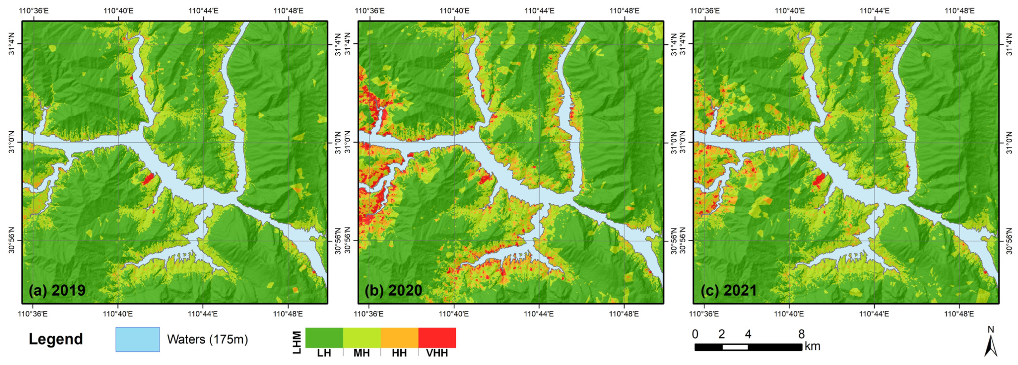
The dynamic LHM of the study area (Figure 9) can be calculated by matrix overlaying the deformation map from 2019 to 2021 and the preliminary LHM (Scenario B) according to Table 1. The area of VHH in the study area was smallest in 2019 and largest in 2020. According to the landslide inventory, the number of landslides in 2020 was the highest, and it was the lowest in 2019, which was consistent with the evaluation results.

5. Discussion

5.1. Accuracy Correction of Hazard Assessment Considering Deformation

In the preliminary LHM (Scenario B), there were 40,990 grids in H4, accounting for 5.88% of the entire study area. However, there were some false-positive errors in the evaluation results. For example, the Xintan landslide in the southeastern part of the study area showed very-high-hazard (H4) classification. With years of continuous engineering management, GPS monitoring data in recent years showed that it was generally stable. Therefore, the hazard level in this area should be reduced. After introducing slope deformation for dynamic LHM, this type of error has been effectively corrected. The Xintan landslide appeared in the LH or MH state. As shown in

Table 7. Comparison of LHM.

Landslide Hazard Level	Preliminary LHM		Dynamic LHM
	Scenario B		2019		2020		2021
	Grids	%	Grids	%	Grids	%	Grids	%
LH	530,585	76.11	546,267	78.36	481,268	69.04	503,123	72.17
MH	57,380	8.23	141,698	20.33	149,580	21.46	163,792	23.50
HH	68,143	9.78	8199	1.18	49,995	7.17	25,810	3.70
VHH	40,990	5.88	934	0.13	16,255	2.33	4373	0.63

, in the dynamic LHM from 2019 to 2021, the numbers of grids in VHH were 934, 16,255, and 4373, accounting for 0.13%, 2.33%, and 0.63% of the study area, respectively. Compared with the preliminary LHM, the areas of VHH decrease, reaching 97.8%, 60.4%, and 89.3%, respectively. The areas of high-hazard zones in these 3 years were reduced by 87.9%, 26.6%, and 62.1%. This significant reduction trend also continued in HH. Dynamic LHM can significantly reduce the scope of high-level landslide hazard zones, greatly reducing unnecessary response and panic.

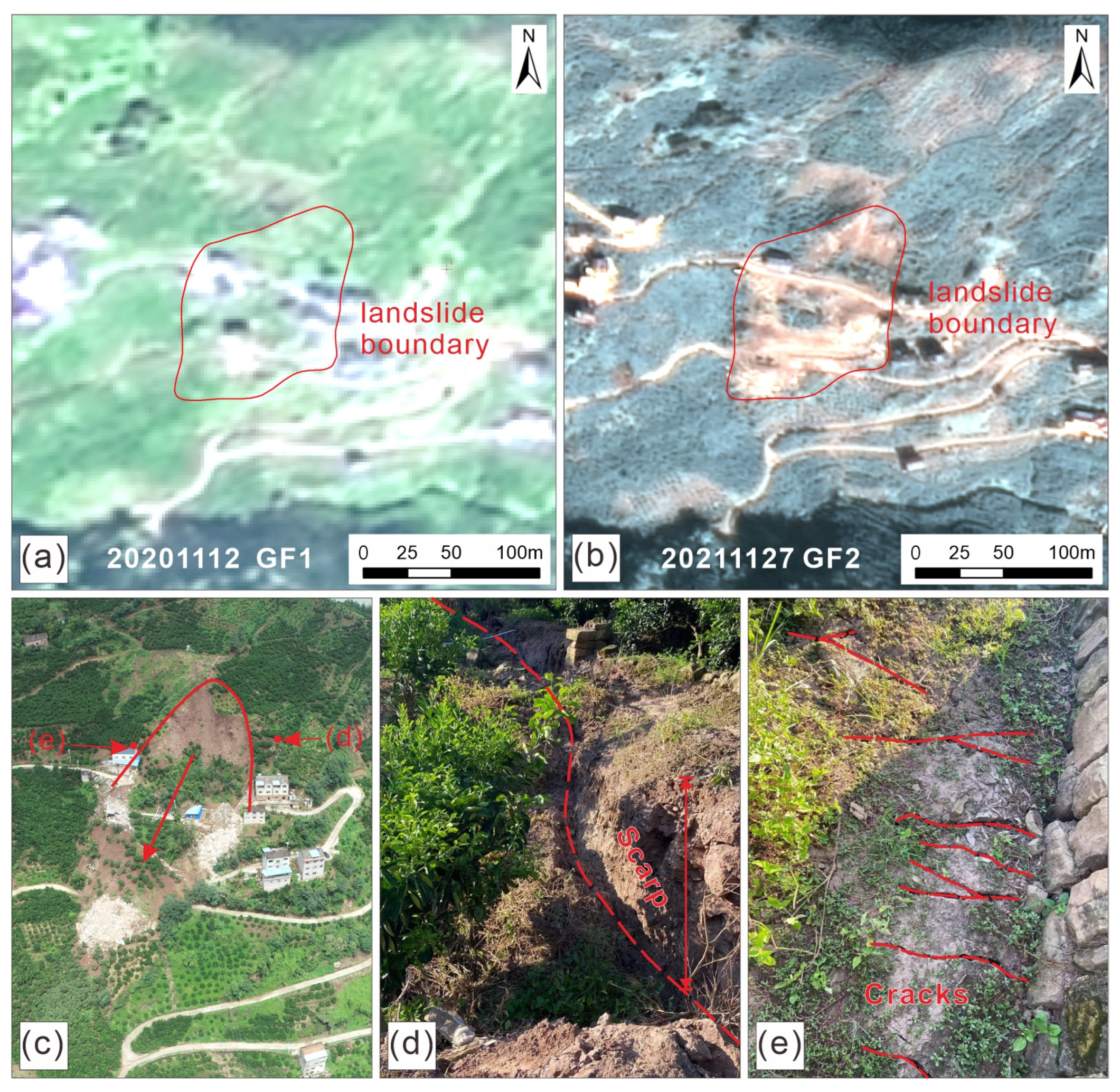
The Kamenziwan (L3 in Figure 2) landslide in 2019, the Tanjiawan (L4 in Figure 2) landslide in 2020, and the Xiaoyantou (L5 in Figure 2) landslide in 2021 (Figure 10a,b) were all in HH or VHH of the corresponding years. The Lianhuatuo (L6 in Figure 2) landslide in the central part of the study area was in VHH for three years from 2019 to 2021. InSAR monitoring showed that the average displacement velocity of the landslide during these three years exceeded 40 mm/year. InSAR monitoring indicates that the Xiaoyantou landslide experienced major deformations in 2020 and 2021 (Figure 10c–e). In the dynamic LHM, it was in MH in 2019, upgraded to HH in 2020, and became VHH in 2021. The dynamic LHM demonstrates great evaluation accuracy. Therefore, the dynamic LHM of regional landslides based on InSAR is a summary of the landslide hazard in this period and a prediction of the landslide hazard for the future.

In terms of the accuracy of hazard assessment, dynamic LHM also showed significant superiority. In 2019, 2020, and 2021, 8, 78 and 38 landslides deformed, respectively. Based on LHM and dynamic LHM, the landslide prediction accuracy in each year can be obtained (

Table 8. Comparison of prediction accuracy between LHM and dynamic LHM.

Years		Total Landslides	Forecast Number	Accuracy
2019	LHM	8	7	87.5%
	Dynamic LHM	8	7	87.5%
2020	LHM	78	68	87.2%
	Dynamic LHM	78	31	39.7%
2021	LHM	38	27	71.1%
	Dynamic LHM	38	14	36.8%

). According to Table 8, in 2019, the accuracies of the two were the same. But in 2020 and 2021, the accuracy of the dynamic LHM improved by 47.5 and 44.3 percentage points, respectively.

The comparison showed that after introducing the deformation interpreted by InSAR for LHM, the area of VHH zoning was reduced, and the false-positive error was also reduced. Dynamic LHM also improved the prediction accuracy. It generally shows an excellent summary and prediction performance and can provide references for landslide early warning and risk management in the study area.

5.2. Different InSAR in High-Vegetation-Coverage Area

In view of the high vegetation coverage in the study area, this research used SAR data of different resolutions and bands (Sentinel-1A, ALOS-2) combined with different methods, such as SBAS-InSAR, PS-InSAR, and D-InSAR.

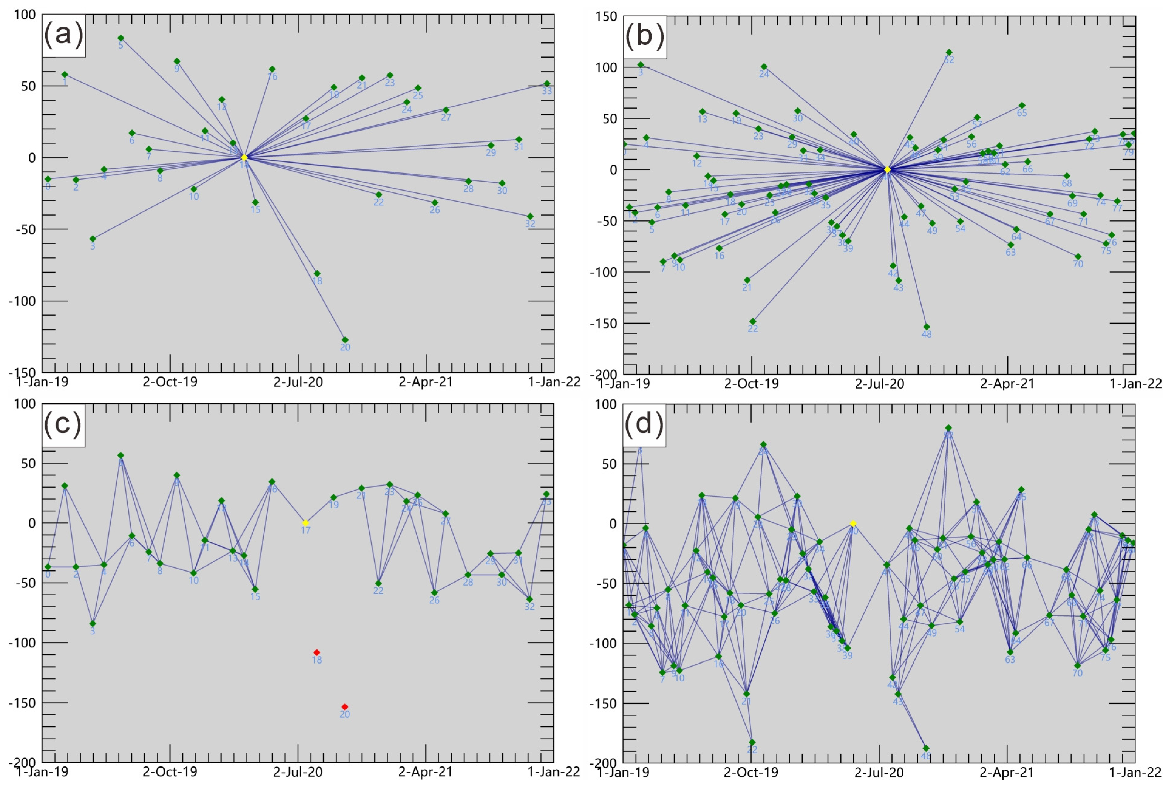
Because there are only two images of ALOS-2 of the study area, only two scenes in 2019 can be used for D-InSAR analysis. The Sentinel-1A datasets had 81 scenes, and two sets of SBAS-InSAR detection and two sets of PS-InSAR detection were performed. During the interpretation process, the time baseline was set to 120 d, the spatial baseline was set to 2%, the coherence coefficient of the PS-InSAR was 0.6, the coherence coefficient of the SBAS-InSAR was 0.1, and the other parameters were set to the default values. In the first group of SBAS-InSAR monitoring, 2 images could not be connected to generate image pairs because of the 2% spatial baseline, and 32 images remained after elimination. After filtering the interferograms, the numbers of connected image pairs of the two sets of SBAS-InSAR were 64 and 314, respectively. The connection of four sets of time series InSAR image pairs is shown in Figure 11.

Five sets of InSAR deformation recognition were conducted in total. There were large differences in the number of deformation points or deformation areas. However, the deformation results were highly consistent. The longer the radar wavelength, the better it can penetrate vegetation. ALOS-2 is in the L-band. Compared with the C-band of Sentinel-1A, ALOS-2 can obtain more deformation information in high-vegetation-coverage areas. The ALOS-2 resolution is 10 m, and the Sentinel-1A resolution is 15 m. Therefore, ALOS-2 data can obtain more information in the same area. D-InSAR obtained 352,586 deformation points carried out by ALOS-2 data, with an area of 277.61km², accounting for 57.18% of the study area. This was much better than the time series InSAR carried out with Sentinel-1A data. This indicates that ALOS-2 performs better in extracting deformation information.

Regarding Sentinel-1A time series measurement, the deformation points calculated by PS-InSAR (34 scenes) were more than those calculated by PS-InSAR (81 scenes). The reason is that the PS-InSAR (34 scenes) had many isolated points with low coherence (0.6), which suggests low reliability. This showed that the interpretation results were positively correlated with the amount of data.

This was also true for the SBAS-InSAR. The more data the SBAS-InSAR used, the more connected image pairs it generated, the more deformation points it could ultimately obtain, and the larger the deformation area. However, even for SBAS-InSAR using 81 scenes of Sentinel-1A data, the generated deformation area was only 68.63km², accounting for only 14.14% of the study area. The deformation areas in the other three sets are all less than 10%. The comparison of the five sets of InSAR is shown in Table 8.

5.2.1. Different InSAR Interpretation Methods in High-Vegetation-Coverage Area

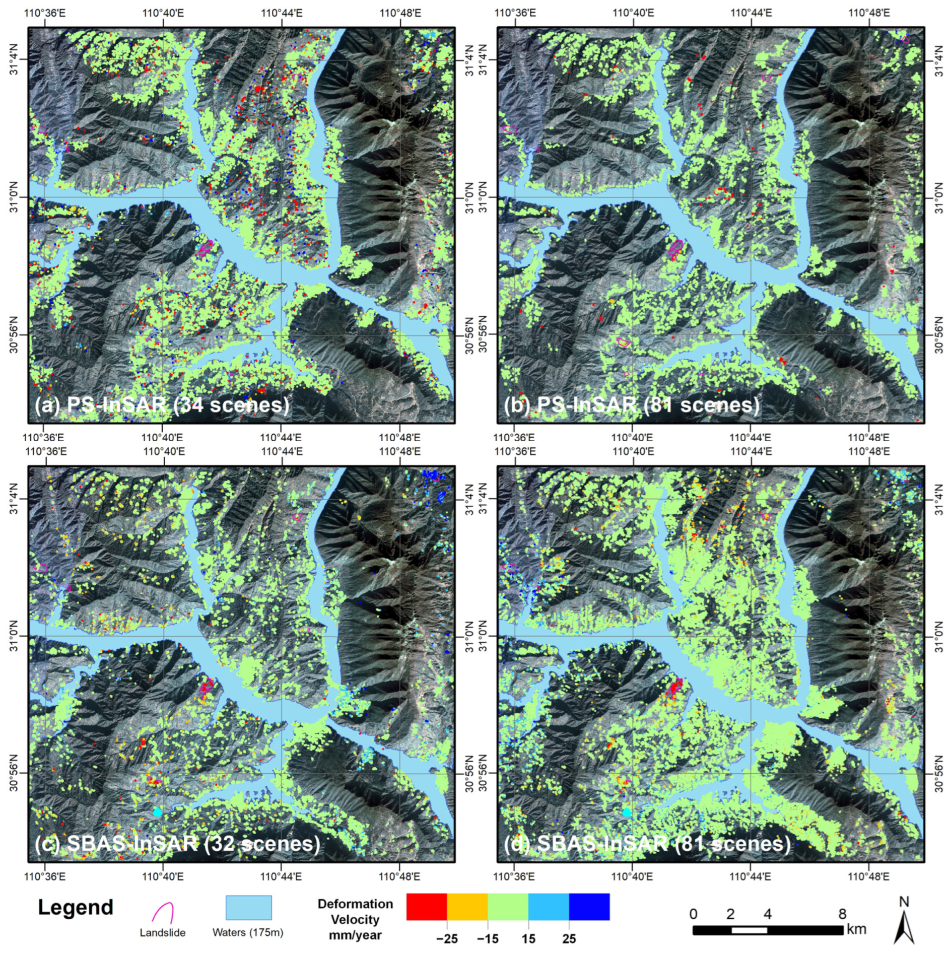
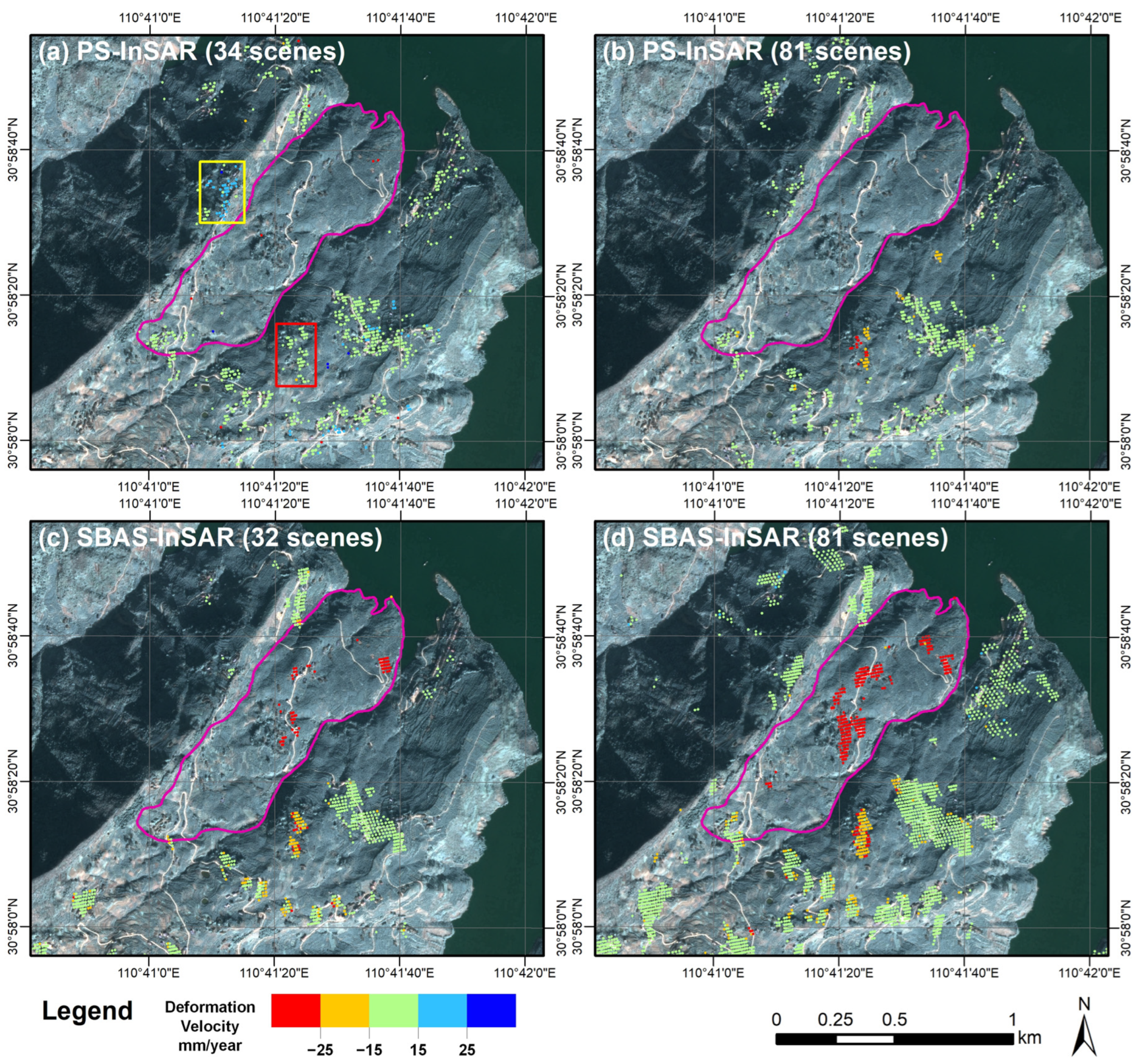
As shown in

Table 9. Information and results of five sets of InSAR.

Algorithm	D-InSAR	PS-InSAR	PS-InSAR	SBAS-InSAR	SBAS-InSAR
Datasets	ALOS-2 Ascending orbit (2 scenes)	Sentinel-1A Ascending orbit (34 scenes)	Sentinel-1A Ascending orbit (81 scenes)	Sentinel-1A Ascending orbit (32 scenes)	Sentinel-1A Ascending orbit (81 scenes)
Connected image pairs	1	33	80	64	314
Total time span	56 days	1068 days	1092 days	1068 days	1092 days
Output coherence threshold	0.3	0.6	0.6	0.1	0.1
Average coherence	0.34	0.71	0.72	0.25	0.3
Deformation points	1,352,586	107,565	92,556	74,495	173,093
Deformation area/km2	277.61	46.14	28.61	28.73	68.63
Area proportion	57.18%	9.50%	5.89%	5.92%	14.14%
Average deformation	0.07mm	−0.98 mm/year	−0.68 mm/year	1.09 mm/year	0.93 mm/year
Maximum	61.97mm	32.01 mm/year	45.89 mm/year	47.49 mm/year	52.73 mm/year
Minimum	−66.03mm	−43.36 mm/year	−57.02 mm/year	−54.21 mm/year	−63.53 mm/year

D-InSAR monitoring time interval was short without annual average deformation velocity.

and Figure 12, the average deformations of the four sets of Sentinel-1A InSAR were close. They could confirm each other in most areas and had the same deformation trends. However, the two sets of PS-InSAR showed abnormal deformation in dense vegetation areas. The SBAS-InSAR incorrectly generated deformation points in waters. Taken together, PS-InSAR is more accurate in open urban areas. And SBAS-InSAR is better in areas with high vegetation coverage.

As shown in Figure 13, in the deformation area of the Lianhuatuo landslide, the PS-InSAR (34 scenes) showed that the deformation in the yellow box was positive deformation, and in the red box it is approximately 0. In the other three sets of InSAR, the deformation in the yellow box is approximately 0, and the deformation in the red box is a negative value. Although there were errors in the first set, the relative deformation of the yellow box and the red box in the four sets of time series InSAR were the same and could be verified with each other. It can be seen from the four sets of results that the two sets of PS-InSAR basically did not obtain the deformation information of the landslide. In comparison, the two sets of SBAS-InSAR both obtained the deformation information, which was highly vegetated. Among them, the deformation results of the SBAS-InSAR (81 scenes) were obviously richer and more accurate. The deformation direction here was roughly the same as the direction of the Sentinel-1A ascending orbit sensor. Therefore, the slow sliding of landslides toward the water surface between 2019 and 2021 showed negative deformation in the line of sight of InSAR deformation interpretation.

5.2.2. Different InSAR Datasets in High-Vegetation-Coverage Area

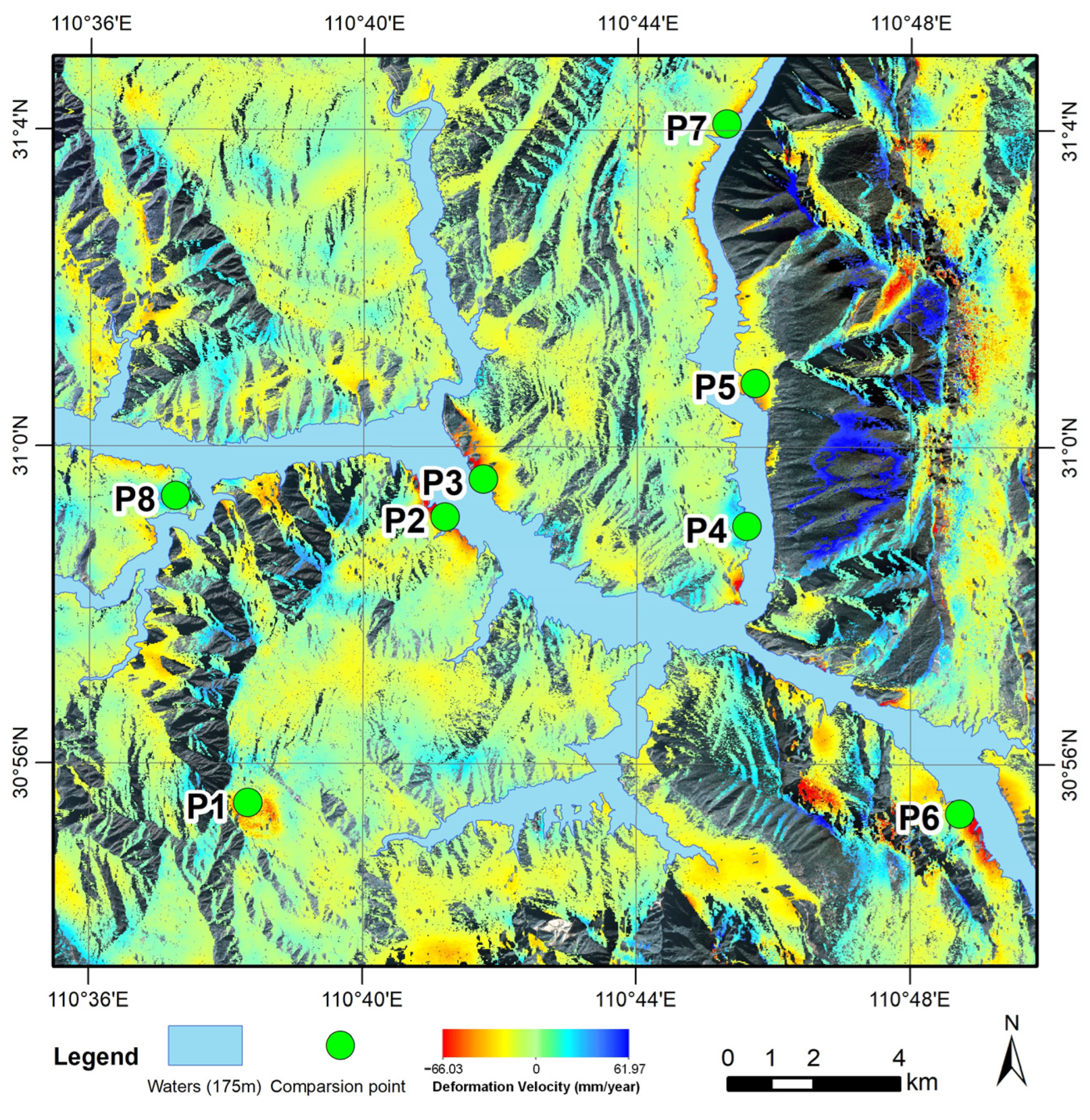
According to the previous comparison, the best detection results of the SBAS-InSAR (81 scenes) were compared with those of ALOS-2. Figure 14 is the D-InSAR deformation interpretation diagram of ALOS-2 data (abnormal deformation results in the perspective shrinkage area were eliminated).

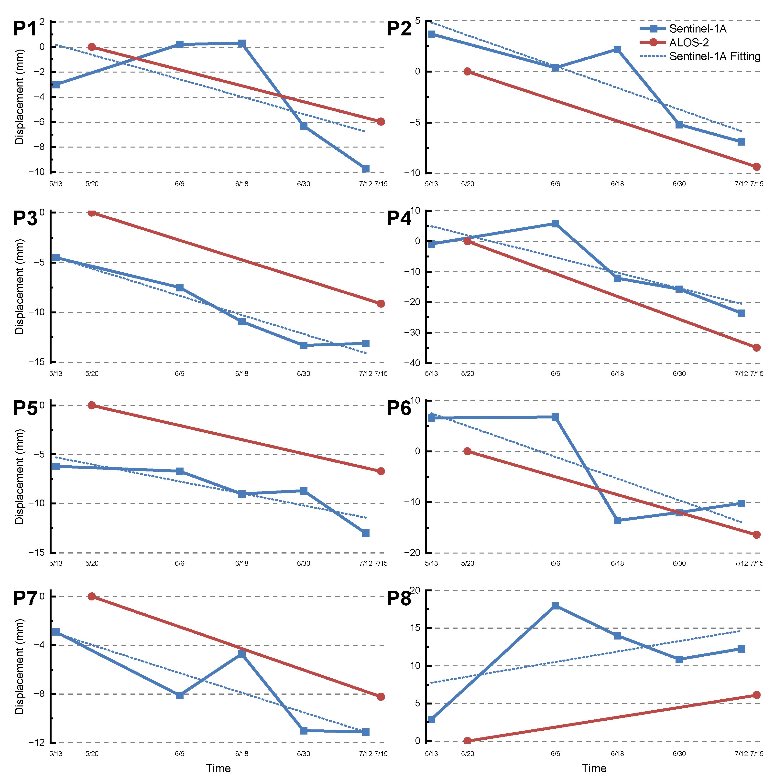
Eight points were randomly selected for comparison. The deformations of the ALOS-2 sets and Sentinel-1A datasets basically confirm each other. Except for a certain error in P4, the deformations of the other points were close or consistent (Figure 15). Because the ALOS-2 datasets had only two scene images, multi-temporal analysis and deformation trend judgment could not be performed.

When monitoring landslides, the D-InSAR was very sensitive to landslides with deformation in the short term. Due to the high vegetation coverage in the study area, it was difficult to obtain effective PS points in many landslides with the PS-InSAR. In this study area, SBAS-InSAR was more suitable for monitoring landslide deformation. Compared with time series InSAR, D-InSAR had lower requirements for data and a shorter processing time. It is suitable for landslides with deformation in the short term but cannot conduct the deformation analysis of long-time sequences. The interpretation method should be chosen according to the time scale of the LHM. Compared with Sentinel-1A data, ALOS-2 data have a higher resolution and longer wavelength. ALOS-2 data have better monitoring results than Sentinel-1A data, but the cost is high. Obtaining the data requires customizing satellite photography plans, which may affect the time limit. When possible, using multi-view ALOS data, shortening the time baseline, and adopting time series interpretation methods can further improve the accuracy of deformation identification and the precision of dynamic LHM. Sentinel-1A data are available for free, with a 12-day spatial baseline, which is relatively stable. From the perspective of availability and economy, Sentinel-1A is more suitable for InSAR monitoring and analysis in the study area.

Therefore, the InSAR deformations used in this study were mainly SBAS-InSAR (81 scenes). In cities and towns, PS-InSAR (81 scenes) data were used for appropriate correction. In other areas, D-InSAR of the ALOS-2 datasets was supplemented as a reference.

6. Conclusions

Dynamic landslide hazard mapping incorporates surface deformation interpreted by multi-InSAR and greatly improves the accuracy. The false-positive rate for VHH was reduced by at least 60%. Taking Zigui, a high-vegetation-coverage area, as the study area, nine factors were selected to finish the landslide susceptibility to obtain the spatial probability. The rainfall exceedance probability was analyzed to calculate the time probability and define the scenarios. Dynamic landslide hazard mapping from 2019 to 2021 was finished according to the surface deformation. The research results show the following:

(1) Dynamic landslide hazard mapping can effectively reduce false-positive errors. Compared with preliminary landslide hazard mapping, while ensuring the assessment’s accuracy, the areas of very-high-hazard zones in 2019, 2020, and 2021 were reduced by 97.8%, 60.4%, and 89.3%, respectively. The high-hazard zones were reduced by 87.9%, 26.6%, and 62.1%, respectively. The landslide hazard in the study area was the highest in 2020. The landslide hazard mapping of each year was in line with the actual situation verified by the field. It can provide effective data support and a reference for landslide early warning and risk management;

(2) This study compared the application effects of two SAR datasets and three InSAR interpretation methods in a high-vegetation-coverage area. It showed that the L-band SAR datasets had a better penetration ability. L-band SAR can penetrate vegetation to obtain more surface deformation information. L-band SAR datasets should be used as much as possible. Long-time series SBAS-InSAR obtained more deformation data in high-vegetation-coverage areas, and the quality of the deformation data was positively correlated with the number of images. D-InSAR was more sensitive to short-term deformation, with a lower requirement of images and fast processing; hence, it is suitable for short-term and emergency hazard mapping.

Dynamic landslide hazard mapping has excellent indicative predicting capabilities. Geological engineers can explore its application in landslide disaster prevention and mitigation, especially landslide early warning. Due to the limitations of the study, the contribution of each factor was not independently analyzed. Further research could differentiate them to obtain a more precise dynamic LHM.

References

1. Gómez, D.; García, E.F.; Aristizábal, E. Spatial and Temporal Landslide Distributions Using Global and Open Landslide Databases. Nat. Hazards 2023, 117, 25–55. [Google Scholar] [CrossRef]
2. Sassa, K. “2006 Tokyo Action Plan”—Strengthening Research and Learning on Landslides and Related Earth System Disasters for Global Risk Preparedness. Landslides 2006, 3, 361–369. [Google Scholar] [CrossRef]
3. Lateltin, O.; Haemmig, C.; Raetzo, H.; Bonnard, C. Landslide Risk Management in Switzerland. Landslides 2005, 2, 313–320. [Google Scholar] [CrossRef]
4. Varnes, D.J. Landslide Hazard Zonation: A Review of Principles and Practice; UNESCO: Paris, France, 1984; Available online: https://unesdoc.unesco.org/ark:/48223/pf0000063038?posInSet=1&queryId=3d365353-6a5e-44a1-89c9-1daec09ab4b9 (accessed on 28 August 2024)ISBN 978-92-3-101895-4.
5. Dhakal, A.; Amada, T.; Aniya, M. Landslide Hazard Mapping and Its Evaluation Using GIS: An Investigation of Sampling Schemes for a Grid-Cell Based Quantitative Method. Photogramm. Eng. Remote Sens. 2000, 66, 981–989. [Google Scholar]
6. Chowdhury, R.; Flentje, P. Effective Urban Landslide Hazard Assessment. Fac. Eng. Inf. Sci.—Pap. Part A 1998, 1–7. Available online: https://ro.uow.edu.au/eispapers/1781 (accessed on 28 August 2024).
7. Glade, T.; Anderson, M.; Crozier, M.J. Landslide Hazard and Risk; John Wiley & Sons Ltd.: Chichester, UK, 2005; Available online: https://onlinelibrary.wiley.com/doi/book/10.1002/9780470012659 (accessed on 28 August 2024)ISBN 0-471-48663-9.
8. Fell, R.; Corominas, J.; Bonnard, C.; Cascini, L.; Leroi, E.; Savage, W.Z. Guidelines for Landslide Susceptibility, Hazard and Risk Zoning for Land-Use Planning. Eng. Geol. 2008, 102, 99–111. [Google Scholar] [CrossRef]
9. Goyes-Peñafiel, P.; Hernandez-Rojas, A. Landslide Susceptibility Index Based on the Integration of Logistic Regression and Weights of Evidence: A Case Study in Popayan, Colombia. Eng. Geol. 2021, 280, 105958. [Google Scholar] [CrossRef]
10. Guo, Z.; Tian, B.; He, J.; Xu, C.; Zeng, T.; Zhu, Y. Hazard Assessment for Regional Typhoon-Triggered Landslides by Using Physically-Based Model—A Case Study from Southeastern China. Georisk Assess. Manag. Risk Eng. Syst. Geohazards 2023, 17, 740–754. [Google Scholar] [CrossRef]
11. Reichenbach, P.; Rossi, M.; Malamud, B.D.; Mihir, M.; Guzzetti, F. A Review of Statistically-Based Landslide Susceptibility Models. Earth-Sci. Rev. 2018, 180, 60–91. [Google Scholar] [CrossRef]
12. Jaiswal, P.; van Westen, C.J. Estimating Temporal Probability for Landslide Initiation along Transportation Routes Based on Rainfall Thresholds. Geomorphology 2009, 112, 96–105. [Google Scholar] [CrossRef]
13. Huabin, W.; Gangjun, L.; Weiya, X.; Gonghui, W. GIS-Based Landslide Hazard Assessment: An Overview. Prog. Phys. Geogr. Earth Environ. 2005, 29, 548–567. [Google Scholar] [CrossRef]
14. Pardeshi, S.D.; Autade, S.E.; Pardeshi, S.S. Landslide Hazard Assessment: Recent Trends and Techniques. SpringerPlus 2013, 2, 523. [Google Scholar] [CrossRef]
15. Del Soldato, M.; Riquelme, A.; Bianchini, S.; Tomàs, R.; Di Martire, D.; De Vita, P.; Moretti, S.; Calcaterra, D. Multisource Data Integration to Investigate One Century of Evolution for the Agnone Landslide (Molise, Southern Italy). Landslides 2018, 15, 2113–2128. [Google Scholar] [CrossRef]
16. Hufschmidt, G.; Crozier, M.J. Evolution of Natural Risk: Analysing Changing Landslide Hazard in Wellington, Aotearoa/New Zealand. Nat. Hazards 2008, 45, 255–276. [Google Scholar] [CrossRef]
17. Rodríguez, C.E.; Bommer, J.J.; Chandler, R.J. Earthquake-Induced Landslides: 1980–1997. Soil. Dyn. Earthq. Eng. 1999, 18, 325–346. [Google Scholar] [CrossRef]
18. Zhou, C.; Cao, Y.; Yin, K.; Intrieri, E.; Catani, F.; Wu, L. Characteristic Comparison of Seepage-Driven and Buoyancy-Driven Landslides in Three Gorges Reservoir Area, China. Eng. Geol. 2022, 301, 106590. [Google Scholar] [CrossRef]
19. Guzzetti, F.; Ardizzone, F.; Cardinali, M.; Rossi, M.; Valigi, D. Landslide Volumes and Landslide Mobilization Rates in Umbria, Central Italy. Earth Planet. Sci. Lett. 2009, 279, 222–229. [Google Scholar] [CrossRef]
20. Lee, S.; Won, J.-S.; Jeon, S.W.; Park, I.; Lee, M.J. Spatial Landslide Hazard Prediction Using Rainfall Probability and a Logistic Regression Model. Math. Geosci. 2015, 47, 565–589. [Google Scholar] [CrossRef]
21. Kirschbaum, D.; Stanley, T. Satellite-Based Assessment of Rainfall-Triggered Landslide Hazard for Situational Awareness. Earth’s Future 2018, 6, 505–523. [Google Scholar] [CrossRef]
22. Gariano, S.L.; Rianna, G.; Petrucci, O.; Guzzetti, F. Assessing Future Changes in the Occurrence of Rainfall-Induced Landslides at a Regional Scale. Sci. Total Environ. 2017, 596–597, 417–426. [Google Scholar] [CrossRef]
23. van Natijne, A.L.; Bogaard, T.A.; van Leijen, F.J.; Hanssen, R.F.; Lindenbergh, R.C. World-Wide InSAR Sensitivity Index for Landslide Deformation Tracking. Int. J. Appl. Earth Obs. Geoinf. 2022, 111, 102829. [Google Scholar] [CrossRef]
24. Zhou, C.; Cao, Y.; Gan, L.; Wang, Y.; Motagh, M.; Roessner, S.; Hu, X.; Yin, K. A Novel Framework for Landslide Displacement Prediction Using MT-InSAR and Machine Learning Techniques. Eng. Geol. 2024, 334, 107497. [Google Scholar] [CrossRef]
25. Zhou, C.; Cao, Y.; Hu, X.; Yin, K.; Wang, Y.; Catani, F. Enhanced Dynamic Landslide Hazard Mapping Using MT-InSAR Method in the Three Gorges Reservoir Area. Landslides 2022, 19, 1585–1597. [Google Scholar] [CrossRef]
26. Wright, T.J.; Parsons, B.E.; Lu, Z. Toward Mapping Surface Deformation in Three Dimensions Using InSAR. Geophys. Res. Lett. 2004, 31, 1–5. [Google Scholar] [CrossRef]
27. Casu, F.; Buckley, S.M.; Manzo, M.; Pepe, A.; Lanari, R. Large Scale InSAR Deformation Time Series: Phoenix and Houston Case Studies. In Proceedings of the 2005 IEEE International Geoscience and Remote Sensing Symposium, IGARSS ’05, Seoul, Republic of Korea, 29 July 2005; Volume 7, pp. 5240–5243. [Google Scholar] [CrossRef]
28. Ferretti, A.; Prati, C.; Rocca, F. Analysis of Permanent Scatterers in SAR Interferometry. In Proceedings of the IGARSS 2000. IEEE 2000 International Geoscience and Remote Sensing Symposium. Taking the Pulse of the Planet: The Role of Remote Sensing in Managing the Environment. Proceedings (Cat. No.00CH37120), Honolulu, HI, USA, 24–28 July 2000; Volume 2, pp. 761–763. [Google Scholar] [CrossRef]
29. Berardino, P.; Fornaro, G.; Lanari, R.; Sansosti, E. A New Algorithm for Surface Deformation Monitoring Based on Small Baseline Differential SAR Interferograms. IEEE Trans. Geosci. Remote Sens. 2002, 40, 2375–2383. [Google Scholar] [CrossRef]
30. García-Davalillo, J.C.; Herrera, G.; Notti, D.; Strozzi, T.; Álvarez-Fernández, I. DInSAR Analysis of ALOS PALSAR Images for the Assessment of Very Slow Landslides: The Tena Valley Case Study. Landslides 2014, 11, 225–246. [Google Scholar] [CrossRef]
31. Herrera, G.; Gutiérrez, F.; García-Davalillo, J.C.; Guerrero, J.; Notti, D.; Galve, J.P.; Fernández-Merodo, J.A.; Cooksley, G. Multi-Sensor Advanced DInSAR Monitoring of Very Slow Landslides: The Tena Valley Case Study (Central Spanish Pyrenees). Remote Sens. Environ. 2013, 128, 31–43. [Google Scholar] [CrossRef]
32. Yazici, B.V.; Tunc Gormus, E. Investigating Persistent Scatterer InSAR (PSInSAR) Technique Efficiency for Landslides Mapping: A Case Study in Artvin Dam Area, in Turkey. Geocarto Int. 2022, 37, 2293–2311. [Google Scholar] [CrossRef]
33. Oliveira, S.C.; Zêzere, J.L.; Catalão, J.; Nico, G. The Contribution of PSInSAR Interferometry to Landslide Hazard in Weak Rock-Dominated Areas. Landslides 2015, 12, 703–719. [Google Scholar] [CrossRef]
34. Li, Y.; Feng, X.; Li, Y.; Jiang, W.; Yu, W. Detection and Analysis of Potential Landslides Based on SBAS-InSAR Technology in Alpine Canyon Region. Env. Sci. Pollut. Res. 2024, 31, 6492–6510. [Google Scholar] [CrossRef]
35. Dwivedi, R.S.; Rao, B.R.M.; Kushwaha, S.P.S. The Utility of Day-and-Night Observation and Cloud-Penetration Capability of ERS-1 SAR Data for Detection of Wetlands. Geocarto Int. 2000, 15, 7–12. [Google Scholar] [CrossRef]
36. Liang, J.; Dong, J.; Zhang, S.; Zhao, C.; Liu, B.; Yang, L.; Yan, S.; Ma, X. Discussion on InSAR Identification Effectivity of Potential Landslides and Factors That Influence the Effectivity. Remote Sens. 2022, 14, 1952. [Google Scholar] [CrossRef]
37. Zhang, B.; Wu, S.; Ding, X.; Wang, C.; Zhu, J.; Li, Q. Use of Multiplatform SAR Imagery in Mining Deformation Monitoring with Dense Vegetation Coverage: A Case Study in the Fengfeng Mining Area, China. Remote Sens. 2021, 13, 3091. [Google Scholar] [CrossRef]
38. Walker, W.S.; Kellndorfer, J.M.; LaPoint, E.; Hoppus, M.; Westfall, J. An Empirical InSAR-Optical Fusion Approach to Mapping Vegetation Canopy Height. Remote Sens. Environ. 2007, 109, 482–499. [Google Scholar] [CrossRef]
39. Oveisgharan, S.; Saatchi, S.S.; Hensley, S. Sensitivity of Pol-InSAR Measurements to Vegetation Parameters. IEEE Trans. Geosci. Remote Sens. 2015, 53, 6561–6572. [Google Scholar] [CrossRef]
40. Maghsoudi, Y.; van der Meer, F.; Hecker, C.; Perissin, D.; Saepuloh, A. Using PS-InSAR to Detect Surface Deformation in Geothermal Areas of West Java in Indonesia. Int. J. Appl. Earth Obs. Geoinf. 2018, 64, 386–396. [Google Scholar] [CrossRef]
41. Chen, L.; Van Westen, C.J.; Hussin, H.; Ciurean, R.L.; Turkington, T.; Chavarro-Rincon, D.; Shrestha, D.P. Integrating Expert Opinion with Modelling for Quantitative Multi-Hazard Risk Assessment in the Eastern Italian Alps. Geomorphology 2016, 273, 150–167. [Google Scholar] [CrossRef]
42. Shano, L.; Raghuvanshi, T.K.; Meten, M. Landslide Susceptibility Evaluation and Hazard Zonation Techniques—A Review. Geoenviron. Disasters 2020, 7, 18. [Google Scholar] [CrossRef]
43. Medina, V.; Hürlimann, M.; Guo, Z.; Lloret, A.; Vaunat, J. Fast Physically-Based Model for Rainfall-Induced Landslide Susceptibility Assessment at Regional Scale. CATENA 2021, 201, 105213. [Google Scholar] [CrossRef]
44. Breiman, L. Random Forests. Mach. Learn. 2001, 45, 5–32. [Google Scholar] [CrossRef]
45. Shuo, Y.; Deying, L.; Liangxuan, Y.; Yuan, H.; Mingzhe, W. Landslide Susceptibility Assessment in High and Steep Bank Slopes along Wujiang River Based on Random Forest Model. Saf. Environ. Eng. 2021, 28, 131–138. [Google Scholar] [CrossRef]
46. Kullback, S.; Leibler, R.A. On Information and Sufficiency. Ann. Math. Stat. 1951, 22, 79–86. [Google Scholar] [CrossRef]
47. Ceriani, L.; Verme, P. The Origins of the Gini Index: Extracts from Variabilità e Mutabilità (1912) by Corrado Gini. J. Econ. Inequal. 2012, 10, 421–443. [Google Scholar] [CrossRef]
48. Gumbel, E.J. Statistics of Extremes; Columbia University Press: New York, NY, USA, 2019; Available online: https://www.degruyter.com/document/doi/10.7312/gumb92958/html (accessed on 28 August 2024)ISBN 978-0-231-89131-8.
49. Althuwaynee, O.F.; Pradhan, B.; Ahmad, N. Estimation of Rainfall Threshold and Its Use in Landslide Hazard Mapping of Kuala Lumpur Metropolitan and Surrounding Areas. Landslides 2015, 12, 861–875. [Google Scholar] [CrossRef]
50. Gabriel, A.K.; Goldstein, R.M.; Zebker, H.A. Mapping Small Elevation Changes over Large Areas: Differential Radar Interferometry. J. Geophys. Res. Solid. Earth 1989, 94, 9183–9191. [Google Scholar] [CrossRef]
51. Chao, Z. Landslide Identification and Prediction with the Application of Time Series InSAR. Ph.D. Thesis, China University of Geosciences, Wuhan, China, 2018. Available online: https://kns.cnki.net/KCMS/detail/detail.aspx?dbcode=CDFD&dbname=CDFDLAST2019&filename=1019826173.nh&v= (accessed on 28 August 2024).
52. Hungr, O.; Leroueil, S.; Picarelli, L. The Varnes Classification of Landslide Types, an Update. Landslides 2014, 11, 167–194. [Google Scholar] [CrossRef]
53. She, X.; Li, D.; Yang, S.; Xie, X.; Sun, Y.; Zhao, W. Landslide Hazard Assessment for Wanzhou Considering the Correlation of Rainfall and Surface Deformation. Remote Sens. 2024, 16, 1587. [Google Scholar] [CrossRef]
54. Hanley, J.A.; McNeil, B.J. A Method of Comparing the Areas under Receiver Operating Characteristic Curves Derived from the Same Cases. Radiology 1983, 148, 839–843. [Google Scholar] [CrossRef]
55. Manconi, A. How Phase Aliasing Limits Systematic Space-Borne DInSAR Monitoring and Failure Forecast of Alpine Landslides. Eng. Geol. 2021, 287, 106094. [Google Scholar] [CrossRef]
Figure 1. Dynamic LHM workflow.
Remotesensing 16 03229 g001
Figure 2. (a) Zigui County in China; (b) study area in Zigui County; (c) landslide map of study area.
Remotesensing 16 03229 g002
Figure 3. Evaluation factors of LSM: (a) Elevation; (b) Slope; (c) Aspect; (d) TRI; (e) Curvature; (f) Plane Curvature; (g) Section Curvature; (h) Lithology; (i) Distance to Fault; (j) TWI; (k) SPI; (l) Distance to River.
Remotesensing 16 03229 g003
Figure 4. IGR of LSM factors.
Remotesensing 16 03229 g004
Figure 5. LSM of the study area.
Remotesensing 16 03229 g005
Figure 6. Preliminary LHM of the study area in different scenarios (a) Scenario A; (b) Scenario B; (c) Scenario C; (d) Scenario D.
Remotesensing 16 03229 g006
Figure 7. Visibility graph of the SAR datasets.
Remotesensing 16 03229 g007
Figure 8. Deformation maps of the study area from 2019 to 2021 by multi-InSAR: (a) 2019; (b) 2020; (c) 2021.
Remotesensing 16 03229 g008
Figure 9. Dynamic LHM in the study area from 2019 to 2021: (a) 2019; (b) 2020; (c) 2021.
Remotesensing 16 03229 g009
Figure 10. Photos of Xiaoyantou landslide: (a) landslide image on 12 November 2020, by GaoFeng-1; (b) landslide failure image on 27 November 2021, by GaoFeng-2; (c) landslide failure photo on August 20, 2021; (d) scarp on landslide crown; (e) cracks on landslide right edge.
Remotesensing 16 03229 g010
Figure 11. Time series InSAR spatiotemporal connection diagram: (a) PS-InSAR (34 scenes); (b) PS-InSAR (81 scenes); (c) SBAS-InSAR (32 scenes); (d) SBAS-InSAR (81 scenes).
Remotesensing 16 03229 g011
Figure 12. Comparison of Sentinel-1A time series InSAR interpretation results: (a) PS-InSAR (34 scenes); (b) PS-InSAR (81 scenes); (c) SBAS-InSAR (32 scenes); (d) SBAS-InSAR (81 scenes).
Remotesensing 16 03229 g012
Figure 13. Comparison of Sentinel-1A time series InSAR interpretation results of Lianhuatuo landslide: (a) PS-InSAR (34 scenes); (b) PS-InSAR (81 scenes); (c) SBAS-InSAR (32 scenes); (d) SBAS-InSAR (81 scenes).
Remotesensing 16 03229 g013
Figure 14. Deformation of ALOS-2 data by D-InSAR.
Remotesensing 16 03229 g014
Figure 15. Interpretation result comparison of Sentinel-1A and ALOS-2.
Remotesensing 16 03229 g015