Incoherent Detection Performance Analysis of the Distributed Multiple-Input Multiple-Output Radar for Rice Fluctuating Targets

Abstract

Utilizing spatial diversity, the distributed multiple-input multiple-output (MIMO) radar has the potential advantage of improving system detection performance. In this paper, the incoherent detection performance of distributed multiple-input multiple-output (MIMO) radars is investigated for Rice fluctuating targets. To calculate the incoherent detection probability, the moment generating function (MGF) of the Rice variable is expanded as the infinite series form. By inverting the product of MGFs of multiple independent Rice variables, new closed-form expressions for the probability density function (PDF) of the sum of independent and weighted squares of Rice variables are proposed. The proposed PDF expression for the sum of independent, non-identically distributed (i.n.i.d.) Rice variables involves an infinite series in terms of the confluent Lauricella function. Specially, the PDF for the sum of independent identically distributed (i.i.d.) Rice is expressed as the confluent hypergeometric function-based infinite series. In addition, the uniform convergence of the proposed PDF expression is also validated. Using this proposed expression, the closed-form and approximate expressions of the incoherent detection probability of MIMO radar are derived, respectively. Numerically evaluated results are illustrated and compared with Monte Carlo (MC) simulations to validate the accuracy of the derivations.

1. Introduction

Over the last two decades, the distributed multiple-input multiple-output (MIMO) radar has attracted significant attention [1,2,3,4,5,6,7,8]. The distributed MIMO radar utilizes widely spaced transmitters and receivers to observe a target from several aspect angles simultaneously. Capitalizing on the spatial diversity of the target’s radar cross-section (RCS), the distributed MIMO radar can oppose the target scintillations and improve the system’s performance in many aspects, such as target detection [9,10,11,12,13,14], target localization [15,16,17], target tracking, etc. Based on the processing method employed, the distributed MIMO radar can be classified into coherent and non-coherent distributed MIMO radars.

Even though coherent processing exhibits superior detection performance in comparison to noncoherent processing, achieving time synchronization and phase synchronization between the transmitters and receivers poses a significant challenge for a coherent distributed MIMO radar [18,19]. In addition, the averaged likelihood ratio (ALR) of the coherent distributed MIMO radar using a Bayesian approach needs to be computed using overly complex integrals [20,21]. Hence, noncoherent processing is usually employed in practical scenarios. For instance, the joint estimation of target location and velocity using the noncoherent MIMO radar for a complex Gaussian extended target is researched in [22]. The moving target localization of the noncoherent MIMO radar system is analyzed using an improved method in [23]. In [24], detecting and localizing multiple targets in a homogeneous noise environment simultaneously is discussed for the noncoherent MIMO radar system.

The detection probability, a critical criterion, is frequently employed to assess the effectiveness of the noncoherent MIMO radar in detecting targets. As applications, the noncoherent detection probability of the distributed MIMO radar for the nonfluctuating targets is analyzed to realize the optimal antenna placement in [25]. In practical scenarios, the detected target is a fluctuating target that conforms to a particular distribution. Typical fluctuating target models include the Swerling-Chi model, the Weibull model, the lognormal model, etc. It has been proven that the optimal detector of the distributed MIMO radar under the Swerling-I fluctuation model is the noncoherent detector [9]. The noncoherent detection probability of the distributed MIMO radar for the Swerling-I model is derived in [9]. The detection performance of the noncoherent distributed MIMO radar for the spatially correlated Swerling-Chi fluctuating targets is analyzed in [26]. Compared with the above fluctuating models, the Rice distribution model is widely used for describing the radar cross section (RCS) characteristics of targets combined by one dominant scatter and many small independent scatters, such as an aircraft probed from the wing edges aspect [27,28]. As an application, the Rice distribution is used to describe the RCS characteristics of the double-ended cone target and the hollow cylinder target [27].

In this paper, the incoherent detection performance of MIMO radar for the Rice fluctuating targets is discussed. The signal-to-noise ratio (SNR) of the test statistic at the incoherent detector output requires the determination of the distribution of the sum of independent and weighted squares of Rice variables. The main contribution of this paper is shown as follows:

• A new closed-form expression of the sum of independent and weighted squares of Rice variables is proposed in terms of the infinite series involving the confluent Lauricella function.
• For the the independent identically distributed (i.i.d.) Rice case, the proposed PDF expression is reduced to the infinite series involving the confluent hypergeometric function.
• The uniform convergence of this closed-form expression is also analyzed.
• The proposed expression is exploited to evaluate the detection probability of MIMO radar for the Rice fluctuating targets.

It is to be noted that this paper mainly focuses on the incoherent detection performance of MIMO radar for the single pulse case, and the derived results can be extended to the multiple pulse case directly.

This paper is organized as follows. Section 2 describes the incoherent detector model of MIMO radar. In Section 3, the closed-form expression of the probability density function (PDF) for the sum of independent and weighted squares of Rice variables is proposed. In Section 4, the proposed PDF is applied to obtain the detection probability of MIMO radar for the Rice fluctuating targets. Section 5 presents the numerical results, and the final conclusions are provided in Section 6.

2. System Model

Assume that the distributed MIMO radar system contains M transmitters and N receivers. Suppose that the ith transmitter transmits a signal $\sqrt{P/M}{s}_i\left(t\right),i=1,\cdots ,M$, where $\mathcal{T}$ is the duration of the normalized signal $s_i\left(t\right)$ (i.e., ${\int }_{\mathcal{T}}{\left|s_i\left(t\right)\right|}^{2}dt=1$) and P is the total transmitted power [5]. In addition, it is supposed that all the transmitted signals are approximately maintain orthogonality for different mutual delay $\tau$, such that ${\int }_{\mathcal{T}}{s}_i\left(t\right)s_k^{*}(t-\tau )dt=0$ for $i\ne k$. The received signal of the jth receiver can be expressed as

$$\begin{array}{c}{r}_j\left(t\right)=\sqrt{P/M}\sum _{i=1}^M{c}_{ji}{s}_i(t-{\tau }_{ji})+n_j\left(t\right)\hfill \end{array}$$

(1)

where ${\tau }_{ji}$ is the time delay and $n_j\left(t\right)$ is a zero-mean, complex Gaussian noise with the distribution $n_j\left(t\right)\sim \mathcal{CN}(0,{\sigma }_n^2)$. And $c_{ji}={\alpha }_{ji}{e}^{j{\phi }_{ji}}$ is the equivalent “channel” scattering coefficient between the ith transmitter, the target and the jth receiver with the amplitude ${\alpha }_{ji}$, and the phase ${\phi }_{ji}$.

Moreover, it is assumed that ${\phi }_{ji}$ is uniformly distributed in $[0,2\pi ]$, and ${\alpha }_{ji}$ is Rice distributed with the PDF given by [29]

$$\begin{array}{cc}{f}_{{\alpha }_{ji}}\left(\alpha \right)\hfill & ={\displaystyle \frac{2(1+k_{ji})\alpha }{{\Omega }_{ji}}}{e}^{-k_{ji}-{\displaystyle \frac{(1+k_{ji})}{{\Omega }_{ji}}}{\alpha }^2}{I}_0\left[2\alpha \sqrt{{\displaystyle \frac{k_{ji}(1+k_{ji})}{{\Omega }_{ji}}}}\right]\hfill \end{array}$$

(2)

where $k_{ji}$ is the shape parameter, ${\Omega }_{ji}$ is the scale parameter denoted as ${\Omega }_{ji}=\mathbb{E}\left[{\alpha }_{ji}^2\right]$, $\mathbb{E}[·]$ is the expectation operator, and $I_0(·)$ is the modified Bessel function of the first kind of order 0.

By applying the matched filter of $s_i\left(t\right)$ to the received signal $r_j\left(t\right)$, the sampling output can be expressed as

$$\begin{array}{cc}{y}_{ji}\hfill & ={\int }_{\mathcal{T}}{r}_j\left(t\right)s_i^{*}(t-{\tau }_{ji})dt\hfill \\ \hfill & =\sqrt{P/M}{\alpha }_{ji}{e}^{j{\phi }_{ji}}+n_{ji}\hfill \end{array}$$

(3)

where $n_{ji}\sim \mathcal{CN}(0,{\sigma }_n^2)$ [5].

The test statistic T of the incoherent detector (i.e., square-law detector) can be expressed as

$$T=\left\{\begin{array}{ccc}\hfill & \sum _{i=1}^M\sum _{j=1}^N{\left|n_{ji}\right|}^2\hfill & {\mathcal{H}}_0\hfill \\ \hfill & \sum _{i=1}^M\sum _{j=1}^N{\left|\sqrt{P/M}{\alpha }_{ji}{e}^{j{\phi }_{ji}}+n_{ji}\right|}^2\hfill & {\mathcal{H}}_1\hfill \end{array}\right.$$

(4)

where $|·|$ is the modulus of a complex number [30]. ${\mathcal{H}}_0$ and ${\mathcal{H}}_1$ refer to the absence and presence of the target, respectively.

Under the hypothesis ${\mathcal{H}}_0$, the test statistic T follows $({\sigma }_n^2/2){\chi }_{\left(2MN\right)}^2$ [9]. And the probability of false alarm $P_{fa}$ is

$$\begin{array}{cc}{P}_{fa}\hfill & =\mathrm{Pr}(T>{\eta }_t|{\mathcal{H}}_0)\hfill \\ \hfill & =\mathrm{Pr}\left({\chi }_{\left(2MN\right)}^2>2{\eta }_t/{\sigma }_n^2\right)\hfill \end{array}$$

(5)

where $\mathrm{Pr}(·)$ is a symbol that denotes the probability depending on the status of a random variable, and the threshold ${\eta }_t$ is determined by $({\sigma }_n^2/2)F_{{\chi }_{\left(2MN\right)}^2}^{-1}(1-P_{fa})$. And $F_{{\chi }_{\left(2MN\right)}^2}^{-1}$ denotes the inverse cumulative distribution function of the chi-square random variable with $2MN$ degrees of freedom [9].

Under hypothesis ${\mathcal{H}}_1$, the probability of detection $P_d$ for the incoherent detector can be expressed as

$$P_d={\int }_0^{\infty }{Q}_{MN}\left(\sqrt{2y},\sqrt{2\eta }\right)f_Y\left(y\right)dy$$

(6)

where $\eta ={\eta }_t/{\sigma }_n^2$, $Q_{\nu }(·,·)$ is the generalized Marcum Q function of $\nu$th order, and $f_Y\left(y\right)$ is the PDF of the variable

$$\begin{array}{c}Y=\sum _{i=1}^M\sum _{j=1}^N{\displaystyle \frac{P{\alpha }_{ji}^2}{M{\sigma }_n^2}}.\hfill \end{array}$$

(7)

In addition, Table 1 displays the definitions of all the variables in the distributed MIMO radar system.

Table 1. All of the variables in the distributed MIMO radar system.

Symbol	Definition
P	The total transmitted power
M	The number of transmitters
N	The number of receivers
$c_{ji}$	The target scattering coefficient between the ith transmitter, the target, and the jth receiver
${\alpha }_{ji}$	The target scattering coefficient amplitude between the ith transmitter, the target, and the jth receiver
${\phi }_{ji}$	The target scattering coefficient phase between the ith transmitter, the target, and the jth receiver
$k_{ji}$	The shape parameter of the Rice variable ${\alpha }_{ji}$
${\Omega }_{ji}$	The scale parameter of the Rice variable ${\alpha }_{ji}$
${\sigma }_n^2$	The noise variance
$P_{fa}$	The probability of false alarm
$P_d$	The probability of detection
${\eta }_t$	The threshold

3. PDF of the Variable Y

To predict the detection probability $P_d$, the PDF of Y should be derived. Define $A={\displaystyle \frac{P}{M{\sigma }_n^2}}$. Stack the $H=MN$ parameters ${\alpha }_{ji}$ into a H-dimensional column vector $\mathit{\alpha }$ such that ${\mathit{\alpha }}_{(i-1)N+j}={\alpha }_{ji}$ [31]. Hence, under the hypothesis ${\mathcal{H}}_1$, Y is the summation of H weighted squares of Rice variables ${\left\{A{\mathit{\alpha }}_h^2\right\}}_{h=1}^H$, where $H=MN$. With the change of variables $y_h=A{\mathit{\alpha }}_h^2$, the PDF of $y_h$ is given by

$$\begin{array}{cc}{f}_{y_h}\left(y\right)\hfill & ={\displaystyle \frac{(1+k_h)e^{-k_h}}{A{\Omega }_h}}{e}^{-{\displaystyle \frac{(1+k_h)y}{A{\Omega }_h}}}{I}_0\left[2\sqrt{{\displaystyle \frac{k_h(1+k_h)y}{A{\Omega }_h}}}\right].\hfill \end{array}$$

(8)

With the appropriate variable substitution, the PDF of Y can be expressed as a Laguerre expansion, but with the restrictive uniform convergence [12]. In this section, a new closed-form expression for the PDF of Y is proposed.

The moment generating function (MGF) of $y_h$ can be expressed by [32]

$$\begin{array}{cc}{\mathcal{M}}_{y_h}\left(s\right)\hfill & ={\int }_0^{\infty }{e}^{sy}{f}_{y_h}\left(y\right)dy\hfill \\ \hfill & ={\displaystyle \frac{1+k_h}{1+k_h-sA{\Omega }_h}}\exp \left({\displaystyle \frac{s{k}_{h}A{\Omega }_h}{1+k_h-sA{\Omega }_h}}\right).\hfill \end{array}$$

(9)

Expanding the exponential term in (9) into a power series and rearranging the expanded terms [33], ${\mathcal{M}}_{y_h}\left(s\right)$ in (9) can be rewritten as

$$\begin{array}{cc}{\mathcal{M}}_{y_h}\left(s\right)\hfill & ={\displaystyle \frac{1+k_h}{1+k_h-sA{\Omega }_h}}\sum _{n_h=0}^{\infty }{\displaystyle \frac{1}{n_h!}}{\left({\displaystyle \frac{s{k}_{h}A{\Omega }_h}{1+k_h-sA{\Omega }_h}}\right)}^{n_h}\hfill \\ \hfill & ={\displaystyle \frac{(1+k_h)/s}{(1+k_h)/s-A{\Omega }_h}}\sum _{n_h=0}^{\infty }{\displaystyle \frac{1}{n_h!}}{\left[{\displaystyle \frac{k_{h}A{\Omega }_h}{(1+k_h)/s-A{\Omega }_h}}\right]}^{n_h}\hfill \\ \hfill & =\sum _{n_h=0}^{\infty }{\displaystyle \frac{{\left(k_{h}A{\Omega }_h\right)}^{n_h}}{n_h!}}{\displaystyle \frac{1+k_h}{s}}{\left({\displaystyle \frac{1+k_h}{s}}-A{\Omega }_h\right)}^{-n_h-1}\hfill \\ \hfill & =-\sum _{n_h=0}^{\infty }{\displaystyle \frac{{(-k_h)}^{n_h}}{n_h!}}{\displaystyle \frac{1+k_h}{sA{\Omega }_h}}{\left[1-{\displaystyle \frac{(1+k_h)/\left(A{\Omega }_h\right)}{s}}\right]}^{-n_h-1}.\hfill \end{array}$$

(10)

Due to the independence of H weighted Rice variables ${\left\{y_h\right\}}_{h=1}^H$, the Laplace transform of Y can be expressed as

$$\begin{array}{cc}\mathcal{L}\left[f_Y\left(y\right)\right]\hfill & ={\int }_0^{\infty }{e}^{-sy}{f}_Y\left(y\right)dy={\mathcal{M}}_Y(-s)=\prod _{h=1}^H{\mathcal{M}}_{y_h}(-s)\hfill \end{array}$$

(11)

where ${\mathcal{M}}_Y\left(s\right)$ is the MGF of Y.

Substituting (10) into (11), we obtain the Laplace transform of $f_Y\left(y\right)$ as follows:

$$\begin{array}{c}\mathcal{L}\left[f_Y\left(y\right)\right]=C\sum _{n_1=0}^{\infty }\cdots \sum _{n_H=0}^{\infty }{\displaystyle \frac{{\prod }_{h=1}^H{k}_h^{n_h}}{{\prod }_{h=1}^H{n}_h!}}{(-1)}^{\overline{n}}{\displaystyle \frac{1}{s^H}}{\left(1+{\displaystyle \frac{{\lambda }_1}{s}}\right)}^{-n_1-1}\cdots {\left(1+{\displaystyle \frac{{\lambda }_H}{s}}\right)}^{-n_H-1}\hfill \end{array}$$

(12)

where ${\lambda }_h=(1+k_h)/\left(A{\Omega }_h\right),C={\prod }_{h=1}^H{\lambda }_h$, and $\overline{n}={\sum }_{h=1}^H{n}_h$.

Capitalizing the Laplace transform given in [34] (p. 290, Equation (55)), which has been applied in [35,36,37], the PDF of Y can be derived by inverting (12) term-by-term as follows

$$\begin{array}{cc}{f}_Y\left(y\right)\hfill & ={\mathcal{L}}^{-1}\left[{\mathcal{M}}_Y(-s)\right]\hfill \\ & =C\sum _{n_1=0}^{\infty }\cdots \sum _{n_H=0}^{\infty }{\displaystyle \frac{{\prod }_{h=1}^H{k}_h^{n_h}}{{\prod }_{h=1}^H{n}_h!}}{\displaystyle \frac{{(-1)}^{\overline{n}}}{\Gamma \left(H\right)}}{y}^{H-1}{\Phi }_2^{\left(H\right)}\left(n_1+1,\cdots ,n_H+1;H;-{\lambda }_{1}y,\cdots ,-{\lambda }_{H}y\right)\hfill \end{array}$$

(13)

where $\Gamma (·)$ is the Gamma function and ${\Phi }_2^{\left(H\right)}(·;·;·)$ is the confluent Lauricella function. The ${\Phi }_2^{\left(H\right)}$ function in (13) can be evaluated fast and efficiently by means of a numerical inverse Laplace transform [38].

For a realistic application, the expression (13) is typically evaluated by the finite summations with parameters $n_h,h=1,\cdots ,H$ truncated at $N_h,h=1,\cdots ,H$ with the expression given by

$$\begin{array}{c}{\widehat{f}}_Y\left(y\right)=C\sum _{n_1=0}^{N_1}\cdots \sum _{n_H=0}^{N_H}{\displaystyle \frac{{\prod }_{h=1}^H{k}_h^{n_h}}{{\prod }_{h=1}^H{n}_h!}}{\displaystyle \frac{{(-1)}^{\overline{n}}{y}^{H-1}}{\Gamma \left(H\right)}}{\Phi }_2^{\left(H\right)}\left(n_1+1,\cdots ,n_H+1;H;-{\lambda }_{1}y,\cdots ,-{\lambda }_{H}y\right).\hfill \end{array}$$

(14)

Uniform convergence: when $y\ge 0$, consider a upper bound of the absolute value of the ${\Phi }_2^{\left(H\right)}$ function in (13), which is expressed as

$$\begin{array}{c}|{\Phi }_2^{\left(H\right)}(n_1+1,\cdots ,n_H+1;H;-{\lambda }_{1}y,\cdots ,-{\lambda }_{H}y)|\le {\Phi }_2^{\left(H\right)}(n_1+1,\cdots ,n_H+1;H;0,\cdots ,0).\hfill \end{array}$$

(15)

Define

$$\begin{array}{c}{\nu }_{\mathbf{n}}\left(y\right)=C{\displaystyle \frac{{\prod }_{h=1}^H{k}_h^{n_h}}{{\prod }_{h=1}^H{n}_h!}}{\displaystyle \frac{{(-1)}^{\overline{n}}}{\Gamma \left(H\right)}}{y}^{H-1}{\Phi }_2^{\left(H\right)}(n_1+1,\cdots ,n_H+1;H;-{\lambda }_{1}y,\cdots ,-{\lambda }_{H}y).\hfill \end{array}$$

(16)

Utilizing the identity ${\Phi }_2^{\left(n\right)}({\alpha }_1,\cdots ,{\alpha }_n;\nu ;0,\cdots ,0)=1$ [35] and (15), the following property for the general term of the series in (16) can be achieved as follows:

$$\begin{array}{cc}|{\nu }_{\mathbf{n}}\left(y\right)|\hfill & =C{\displaystyle \frac{{\prod }_{h=1}^H{k}_h^{n_h}}{{\prod }_{h=1}^H{n}_h!}}{\displaystyle \frac{y^{H-1}}{\Gamma \left(H\right)}}\left|{\Phi }_2^{\left(H\right)}(n_1+1,\cdots ,n_H+1;H;-{\lambda }_{1}y,\cdots ,-{\lambda }_{H}y)\right|\hfill \\ \hfill & \le C{\displaystyle \frac{{\prod }_{h=1}^H{k}_h^{n_h}}{{\prod }_{h=1}^H{n}_h!}}{\displaystyle \frac{y^{H-1}}{\Gamma \left(H\right)}}{\Phi }_2^{\left(H\right)}(n_1+1,\cdots ,n_H+1;H;0,\cdots ,0)\hfill \\ \hfill & =C{\displaystyle \frac{{\prod }_{h=1}^H{k}_h^{n_h}}{{\prod }_{h=1}^H{n}_h!}}{\displaystyle \frac{y^{H-1}}{\Gamma \left(H\right)}}\hfill \end{array}$$

(17)

where $\mathbf{n}=\{n_1,\cdots ,n_H\}$.

For all $0\le y\le b$, we can obtain

$$\begin{array}{cc}|{\nu }_{\mathbf{n}}\left(y\right)|\hfill & \le C{\displaystyle \frac{{\prod }_{h=1}^H{k}_h^{n_h}}{{\prod }_{h=1}^H{n}_h!}}{\displaystyle \frac{y^{H-1}}{\Gamma \left(H\right)}}\hfill \\ \hfill & \le C{\displaystyle \frac{{\prod }_{h=1}^H{k}_h^{n_h}}{{\prod }_{h=1}^H{n}_h!}}{\displaystyle \frac{b^{H-1}}{\Gamma \left(H\right)}}.\hfill \end{array}$$

(18)

Based on the fact that

$$\begin{array}{c}\sum _{n_1=0}^{\infty }\cdots \sum _{n_H=0}^{\infty }C{\displaystyle \frac{{\prod }_{h=1}^H{k}_h^{n_h}}{{\prod }_{h=1}^H{n}_h!}}{\displaystyle \frac{b^{H-1}}{\Gamma \left(H\right)}}=C{e}^{{\sum }_{h=1}^H{k}_h}{\displaystyle \frac{b^{H-1}}{\Gamma \left(H\right)}}\hfill \end{array}$$

(19)

and in view of the Weierstrass M-test [39], $f_Y\left(y\right)={\sum }_{\mathbf{n}=0}^{\infty }{\nu }_{\mathbf{n}}\left(y\right)$ converges uniformly in any finite interval of $[0,\infty )$ [40].

If H Rice variables ${\left\{{\mathit{\alpha }}_h\right\}}_{h=1}^H$ are independent and identically distributed (i.i.d) with same parameters k and $\Omega$, the summation of H variables ${\left\{A{\mathit{\alpha }}_h^2\right\}}_{h=1}^H$ will be reduced to ([41], Equation (14))

$$\begin{array}{c}{f}_{Y,iid}\left(y\right)={\lambda }^H\sum _{n_1=0}^{\infty }\cdots \sum _{n_H=0}^{\infty }{\displaystyle \frac{k^{n_1+\cdots +n_H}}{{\prod }_{h=1}^H{n}_h!}}{\displaystyle \frac{{(-1)}^{\overline{n}}}{\Gamma \left(H\right)}}{y}^{H-1}{}_1{F}_1\left(\overline{n}+H;H;-\lambda y\right)\hfill \end{array}$$

(20)

where $\lambda =(1+k)/(A\Omega )$ and ${}_1{F}_1(·;·;·)$ is the confluent hypergeometric function [42].

4. Detection Performance Prediction

In this section, closed-form and approximate expressions of the incoherent detection probability are derived, respectively.

Considering an alternative series form of the Marcum Q function ([40], Equation (14)) and $H=MN$, (6) can be expanded as

$$\begin{array}{c}{P}_d={\int }_0^{\infty }\left\{\sum _{p=0}^{\infty }{e}^{-y}{\displaystyle \frac{y^p}{p!}}{\displaystyle \frac{\Gamma (H+p,\eta )}{\Gamma (H+p)}}\right\}{f}_Y\left(y\right)dy\hfill \end{array}$$

(21)

where $\Gamma (·,·)$ is the upper incomplete gamma function.

Interchanging the order of summation and integration of (21), which is proved in Appendix A, the following identity can be achieved:

$$\begin{array}{cc}\hfill & P_d=\sum _{p=0}^{\infty }{\displaystyle \frac{1}{p!}}{\displaystyle \frac{\Gamma (H+p,\eta )}{\Gamma (H+p)}}\underset{{\mathcal{L}}_p}{\underbrace{{\int }_0^{\infty }{e}^{-y}{y}^p{f}_Y\left(y\right)dy}}.\hfill \end{array}$$

(22)

The integrand ${\mathcal{L}}_p$ in (22) can be expanded as

$$\begin{array}{cc}\hfill & {\mathcal{L}}_p=C{\int }_0^{\infty }\sum _{n_1=0}^{\infty }\cdots \sum _{n_H=0}^{\infty }{\displaystyle \frac{{\prod }_{h=1}^H{k}_h^{n_h}}{{\prod }_{h=1}^H{n}_h!}}{\displaystyle \frac{{(-1)}^{\overline{n}}}{\Gamma \left(H\right)}}{e}^{-y}{y}^{p+H-1}\hfill \\ \hfill & \times {\Phi }_2^{\left(H\right)}\left(n_1+1,\cdots ,n_H+1;H;-{\lambda }_{1}y,\cdots ,-{\lambda }_{H}y\right)dy.\hfill \end{array}$$

(23)

Based on the analysis provided in Appendix B, interchanging the summation and integration in (23) can be guaranteed. Substituting (23) into (22), one can obtain the incoherent detection probability as follows:

$$\begin{array}{cc}\hfill & P_d=C\sum _{p=0}^{\infty }\sum _{n_1=0}^{\infty }\cdots \sum _{n_H=0}^{\infty }{\displaystyle \frac{1}{p!}}{\displaystyle \frac{\Gamma (H+p,\eta )}{\Gamma (H+p)}}{\displaystyle \frac{{\prod }_{h=1}^H{k}_h^{n_h}}{{\prod }_{h=1}^H{n}_h!}}{\displaystyle \frac{{(-1)}^{\overline{n}}}{\Gamma \left(H\right)}}\hfill \\ \hfill & \times {\int }_0^{\infty }{e}^{-y}{y}^{p+H-1}{\Phi }_2^{\left(H\right)}(n_1+1,\cdots ,n_H+1;H;-{\lambda }_{1}y,\cdots ,-{\lambda }_{H}y)dy.\hfill \end{array}$$

(24)

Considering the identity given by [34] (p. 286, Equation (43)), $P_d$ in (24) can be represented as follows:

$$\begin{array}{cc}\hfill & P_d=C\sum _{p=0}^{\infty }\sum _{n_1=0}^{\infty }\cdots \sum _{n_H=0}^{\infty }{\displaystyle \frac{\Gamma (H+p,\eta )}{p!}}{\displaystyle \frac{{\prod }_{h=1}^H{k}_h^{n_h}}{{\prod }_{h=1}^H{n}_h!}}{\displaystyle \frac{{(-1)}^{\overline{n}}}{\Gamma \left(H\right)}}\hfill \\ \hfill & \times F_D^{\left(H\right)}(p+H,n_1+1,\cdots ,n_H+1;H;-{\lambda }_1,\cdots ,-{\lambda }_H)\hfill \end{array}$$

(25)

where $F_D^{\left(n\right)}$ is the Lauricella’s function of the fourth kind [34].

It is to be noted that the $F_D^{\left(n\right)}$ function converges if $\max \left\{\right|{\lambda }_1|,\cdots ,|{\lambda }_H\left|\right\}<1$. However, this condition may not be satisfied in a real scenario. To achieve a convergent form of the $F_D^{\left(n\right)}$ function, consider the transformation of the Lauricella’s function of the fourth kind ([43], Equation (19))

$$\begin{array}{cc}\hfill & F_D^{\left(n\right)}(a,b_1,\cdots ,b_n;c;x_1,\cdots ,x_n)=\left[\prod _{i=1}^n{(1-x_i)}^{-b_i}\right]\hfill \\ \hfill & \times F_D^{\left(n\right)}\left(c-a,b_1,\cdots ,b_n;c;{\displaystyle \frac{x_1}{x_1-1}},\cdots ,{\displaystyle \frac{x_n}{x_n-1}}\right)\hfill \end{array}$$

(26)

and $P_d$ in (25) can be rewritten as

$$\begin{array}{cc}& P_d=C\sum _{p=0}^{\infty }\sum _{n_1=0}^{\infty }\cdots \sum _{n_H=0}^{\infty }{\displaystyle \frac{\Gamma (H+p,\eta )}{p!}}{\displaystyle \frac{{\prod }_{h=1}^H{k}_h^{n_h}}{{\prod }_{h=1}^H{n}_h!}}{\displaystyle \frac{{(-1)}^{\overline{n}}}{\Gamma \left(H\right)}}\hfill \\ & \times \prod _{h=1}^H{(1+{\lambda }_h)}^{-(n_h+1)}{F}_D^{\left(H\right)}\left(-p,n_1+1,\cdots ,n_H+1;H;{\displaystyle \frac{{\lambda }_1}{{\lambda }_1+1}},\cdots ,{\displaystyle \frac{{\lambda }_H}{{\lambda }_H+1}}\right).\hfill \end{array}$$

(27)

In particular, capitalizing the identity ([34], p. 34, Equation (6)), $P_d$ in (27) for the independent and identically distributed MIMO radar channels will be further reduced to

$$\begin{array}{cc}\hfill & P_{d,iid}={\left({\displaystyle \frac{\lambda }{1+\lambda }}\right)}^H\sum _{p=0}^{\infty }\sum _{n_1=0}^{\infty }\cdots \sum _{n_H=0}^{\infty }{\displaystyle \frac{\Gamma (H+p,\eta )}{p!}}\hfill \\ \hfill & \times {\displaystyle \frac{{[k/(1+\lambda )]}^{\overline{n}}}{n_1!\cdots n_H!}}{\displaystyle \frac{{(-1)}^{\overline{n}}}{\Gamma \left(H\right)}}{}_2{F}_1\left[-p,\overline{n}+H;H;{\displaystyle \frac{\lambda }{\lambda +1}}\right]\hfill \end{array}$$

(28)

where ${}_2{F}_1(a,b;c;z)$ is the hypergeometric function [42].

Moreover, the function $F_D^{\left(H\right)}(a,b_1,\cdots ,b_H;c;x_1,\cdots ,x_H)$ is reduced to the Appell hypergeometric function $F_1$ if $H=2$ ([34], p. 22, Equation (2)), which is already implemented in Maple and Mathematica scientific software. Unfortunately, there is no fast numerical evaluation of the function $F_D^{\left(H\right)}$ if $a<0$ and $H>2$. To facilitate the application of detection probability in engineering, a simpler approximation to $P_d$ in (24) is derived in terms of the K-point Gauss–Laguerre quadrature as

$$\begin{array}{cc}{\tilde{P}}_d\hfill & \approx \sum _{p=0}^{\infty }{\displaystyle \frac{1}{p!}}{\displaystyle \frac{\Gamma (H+p,\eta )}{\Gamma (H+p)}}{\mathcal{K}}_p\hfill \end{array}$$

(29)

with ${\mathcal{K}}_p$ given by

$$\begin{array}{cc}{\mathcal{K}}_p\hfill & =\sum _{i=1}^K{\omega }_i{\zeta }_i^p{f}_Y\left({\zeta }_i\right)\hfill \\ \hfill & =C\sum _{i=1}^K\sum _{n_1=0}^{\infty }\cdots \sum _{n_H=0}^{\infty }{\omega }_i{\zeta }_i^{p+H-1}{\displaystyle \frac{{\prod }_{h=1}^H{k}_h^{n_h}}{{\prod }_{h=1}^H{n}_h!}}{\displaystyle \frac{{(-1)}^{\overline{n}}}{\Gamma \left(H\right)}}\hfill \\ \hfill & \times {\Phi }_2^{\left(H\right)}(n_1+1,\cdots ,n_H+1;H;-{\lambda }_1{\zeta }_i,\cdots ,-{\lambda }_H{\zeta }_i)\hfill \end{array}$$

(30)

where ${\left\{{\omega }_i\right\}}_{i=1}^K$ and ${\left\{{\zeta }_i\right\}}_{i=1}^K$ are the associated weights and abscissas ([44], Equation (25.4.45)).

For a realistic application, the expressions (27) and (28) are typically evaluated by the finite summations with parameters p and $n_h,h=1,\cdots ,H$ truncated at $I_p$ and $N_h,h=1,\cdots ,H$, with the expressions given by

$$\begin{array}{cc}& P_d=C\sum _{p=0}^{I_p}\sum _{n_1=0}^{N_1}\cdots \sum _{n_H=0}^{N_H}{\displaystyle \frac{\Gamma (H+p,\eta )}{p!}}{\displaystyle \frac{{\prod }_{h=1}^H{k}_h^{n_h}}{{\prod }_{h=1}^H{n}_h!}}{\displaystyle \frac{{(-1)}^{\overline{n}}}{\Gamma \left(H\right)}}\hfill \\ & \times \prod _{h=1}^H{(1+{\lambda }_h)}^{-(n_h+1)}{F}_D^{\left(H\right)}\left(-p,n_1+1,\cdots ,n_H+1;H;{\displaystyle \frac{{\lambda }_1}{{\lambda }_1+1}},\cdots ,{\displaystyle \frac{{\lambda }_H}{{\lambda }_H+1}}\right)\hfill \end{array}$$

(31)

and

$$\begin{array}{cc}\hfill & P_{d,iid}={\left({\displaystyle \frac{\lambda }{1+\lambda }}\right)}^H\sum _{p=0}^{I_p}\sum _{n_1=0}^{N_1}\cdots \sum _{n_H=0}^{N_H}{\displaystyle \frac{\Gamma (H+p,\eta )}{p!}}\hfill \\ \hfill & \times {\displaystyle \frac{{[k/(1+\lambda )]}^{\overline{n}}}{n_1!\cdots n_H!}}{\displaystyle \frac{{(-1)}^{\overline{n}}}{\Gamma \left(H\right)}}{}_2{F}_1\left[-p,\overline{n}+H;H;{\displaystyle \frac{\lambda }{\lambda +1}}\right].\hfill \end{array}$$

(32)

Similarly, for the realistic application, the expression (29) is evaluated by the finite summations with the expressions given by

$$\begin{array}{cc}{\tilde{P}}_d\hfill & =C\sum _{p=0}^{I_p}\sum _{i=1}^K\sum _{n_1=0}^{N_1}\cdots \sum _{n_H=0}^{N_H}{\displaystyle \frac{1}{p!}}{\displaystyle \frac{\Gamma (H+p,\eta )}{\Gamma (H+p)}}{\omega }_i{\zeta }_i^{p+H-1}\hfill \\ \hfill & \times {\displaystyle \frac{{\prod }_{h=1}^H{k}_h^{n_h}}{{\prod }_{h=1}^H{n}_h!}}{\displaystyle \frac{{(-1)}^{\overline{n}}}{\Gamma \left(H\right)}}{\Phi }_2^{\left(H\right)}(n_1+1,\cdots ,n_H+1;H;-{\lambda }_1{\zeta }_i,\cdots ,-{\lambda }_H{\zeta }_i).\hfill \end{array}$$

(33)

5. Simulation Results

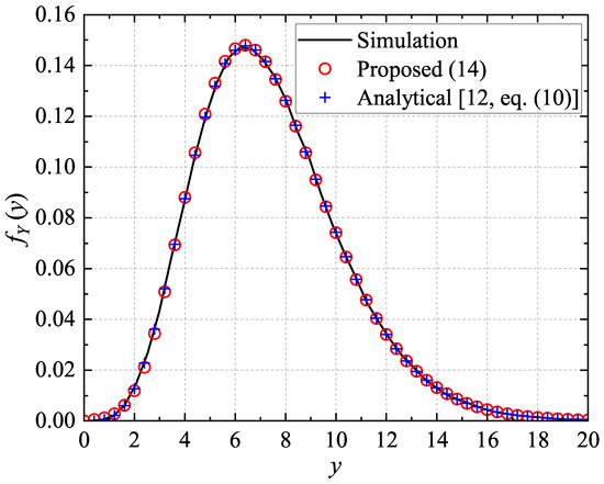
Firstly, the proposed closed-form expression (14) is validated statistically. Without the loss of generality, set the weight $A=1$. Consider four independent Rice variables with parameters $(k_1,k_2,k_3,k_4)=(3,1.5,2.3,1.2)$ and $({\Omega }_1,{\Omega }_2,{\Omega }_3,{\Omega }_4)=(2,2.4,1.6,1.4)$. Figure 1 shows a comparison of the PDF for the sum of the above four squares of Rice variables obtained from the proposed expression (14) with truncated series at $N_i=4$ and $N_i=8,i=1,\cdots ,4$, the analytical expression ([12], Equation (10)), and the histogram of Monte Carlo (MC) simulations with ${10}^6$ independent runs. As expected, a good match is achieved between the proposed expression (14), the analytical expression ([12], Equation (10)), and the MC simulations. Table 2 compares the computation accuracy between the proposed expression (14) and the analytical expression ([12], Equation (10)). It can be found that the relative computation error is less than ${10}^{-2}$.

Figure 1. Comparison between PDFs obtained from the proposed expression (14), the analytical expression ([12], Equation (10)), and the MC simulations.

Table 2. Computation accuracy between the proposed expression (14) and the analytical expression ([12], Equation (10)).

Variable	Proposed (14)	Analytical ([12], Equation (10))
$y=4$	0.088019	0.087541
$y=8$	0.125869	0.126226
$y=12$	0.034027	0.034013

To evaluate the accuracy of the proposed method, the mean square error (MSE) test is employed. The MSE test is defined as

$$\mathrm{MSE}={\displaystyle \frac{{\displaystyle \sum _{i=1}^I}{\left[f_e\left(y_i\right)-f\left(y_i\right)\right]}^2}{I}}$$

(34)

where I is the number of samples, $f_e\left(y_i\right)$ is the empirical distribution function of $y_i$, and $f\left(y_i\right)$ is the PDF of $y_i$ computed using the computed distribution parameters of $y_i$. Table 3 compares the MSE between the proposed expression (14) and the analytical expression ([12], Equation (10)). It can be found that the relative computation error is very small. In addition, increasing the number of truncated terms can reduce the truncation error of the proposed method (14).

Table 3. MSE comparisons between the proposed expression (14) and the analytical expression ([12], Equation (10)).

MSE	Proposed (14) (${\mathit{N}}_{\mathit{i}}=4$)	Proposed (14) (${\mathit{N}}_{\mathit{i}}=8$)	Analytical ([12], Equation (10))
Value	3.1206 $\times {10}^{-7}$	5.1051 $\times {10}^{-8}$	5.1189 $\times {10}^{-8}$

Next, the incoherent detection performance of MIMO radar is evaluated in terms of the receiver operating characteristic (ROC) curves. Define $\rho =P/{\sigma }_n^2$ as the average received SNR and set ${\sigma }_n^2=1$.

For a special case, the MIMO radar is assumed with two transmitters and one receiver with fading parameters $(k_{1,1},k_{1,2})=(1.5,2.1)$ and $({\Omega }_{1,1},{\Omega }_{1,2})=(2,1.4)$. Figure 2 compares the ROC curves of the incoherent detector of MIMO radar under the above Rice scattering scenario obtained by the theoretical results and the MC simulations with different SNRs. For the theoretical results, the values of $P_{fa}$ are obtained by the expression (5). The values of $P_d$ are obtained by the expression (31) with truncated series at $N_1=N_2=6$, $I_p=60$, and the approximate expression (33) with $K=16,N_1=N_2=6$, $I_p=60$, respectively. The numbers of independent trials for simulating $P_{fa}$ and $P_d$ are $100/P_{fa}$ and ${10}^4$ [45]. As expected, the theoretical results match the MC simulation results pretty well.

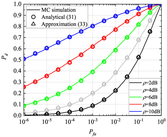
Figure 2. ROC curve comparisons between derived results and MC simulations for the MIMO radar with two transmitters and one receivers.

In addition, the MIMO radar is assumed with $N_t=2$ transmitters and $N_r=1,2,3$ receiver with fading parameters $k_{n,1}=k_{n,2}=1.8,n=1,2,3$ and ${\Omega }_{n,1}={\Omega }_{n,2}=1.6,n=1,2,3$. The number of antenna elements of the MIMO radar is $N=N_t{N}_r$. The average received SNR is set as 5 dB. Figure 3 compares the ROC curves of the incoherent detector of MIMO radar under the above Rice scattering scenario obtained by the theoretical results and the MC simulations with different number of antenna elements. The values of $P_d$ are obtained by the approximate expression (33) with $K=16,N_1=N_2=6$, and $I_p=60$, respectively. It can be found that the probability of detection increases with the increase in the number of antenna elements for a fixed $P_{fa}$.

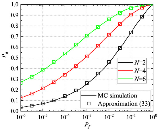
Figure 3. ROC curve comparisons between derived results and MC simulations for the MIMO radar with different number of antenna elements.

Finally, consider the case of MIMO radar with two transmitting antennas and three receiving receiving antennas. The scattering coefficients of the six channels are supposed to be Rice distributed with parameters $k=(1.2,2.1,1.7,2.9,1.1,1.9)$ and $\Omega =(3.2,1.4,1.5,2.3,1.3,2.1)$. ROC curves of the incoherent detector of MIMO radar for the above Rice scattering scenario obtained by Expressions (5) and (33) with $N_i=2,i=1,\cdots ,6$, $I_p=60$, and $K=24$ are plotted in Figure 4. As a comparison, the values of $P_{fa}$ and $P_d$ obtained by the MC simulations are also estimated using $100/P_{fa}$ and ${10}^4$ independent runs, respectively.

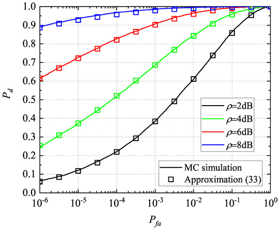
Figure 4. ROC curve comparisons between derived results and MC simulations for the MIMO radar with two transmitters and three receivers.

Again, a tight agreement is obtained between the analytical expression and the MC simulation results. Moreover, at a fixed probability of false alarm, the detection probability increases as the average received SNR increases.

6. Conclusions

The incoherent detection performance of distributed MIMO radar for the Rice fluctuating targets is investigated in this paper. In particular, a new analytical expression for the PDF of the SNR of the incoherent detector output has been presented. Numerical results are provided to verify the accuracy of the derivations. In addition, the closed-form and approximate expressions for the incoherent detection probability are derived to demonstrate the effect of the average received SNR on the incoherent detection performance.

References

- Wang, H.; Xu, L.; Yan, Z.; Gulliver, T.A. Low-complexity MIMO-FBMC sparse channel parameter estimation for industrial big data communications. IEEE Trans. Ind. Inform. 2021, 17, 3422–3430. [Google Scholar] [CrossRef]
- Wen, F.; Shi, J.; Lin, Y.; Cui, G.; Yuen, C.; Sari, H. Joint DOD and DOA estimation for NLOS target using IRS-aided bistatic MIMO radar. IEEE Trans. Veh. Technol. 2024. [Google Scholar] [CrossRef]
- Xu, Z.; Fan, C.; Huang, X. MIMO radar waveform design for multipath exploitation. IEEE Trans. Signal Process. 2021, 69, 5359–5371. [Google Scholar] [CrossRef]
- Ma, Y.; Miao, C.; Long, W.; Zhang, R.; Chen, Q.; Zhang, J.; Wu, W. Time-modulated arrays in scanning mode using wideband signals for range-doppler estimation with time-frequency filtering and fusion. IEEE Trans. Aerosp. Electron. Syst. 2024, 60, 980–990. [Google Scholar] [CrossRef]
- Haimovich, A.M.; Blum, R.S.; Cimini, L.J. MIMO radar with widely separated antennas. IEEE Signal Process. Mag. 2008, 25, 116–129. [Google Scholar] [CrossRef]
- Kalkan, Y. 20 years of MIMO radar. IEEE Aerosp. Electron. Syst. Mag. 2024, 39, 28–35. [Google Scholar] [CrossRef]
- Sun, S.; Hu, Y.; Mishra, K.V.; Petropulu, A.P. Widely separated MIMO radar using matrix completion. IEEE Trans. Radar Syst. 2024, 2, 180–196. [Google Scholar] [CrossRef]
- Luo, D.; Wen, G.; Liang, Y.; Zhu, L.; Song, H. Beam scheduling for early warning with distributed MIMO radars. IEEE Trans. Aerosp. Electron. Syst. 2023, 59, 6044–6058. [Google Scholar] [CrossRef]
- Fishler, E.; Haimovich, A.; Blum, R.; Cimini, R.; Chizhik, D.; Valenzuela, R. Spatial diversity in radars–Models and detection perofrmance. IEEE Trans. Signal Process. 2006, 54, 823–838. [Google Scholar] [CrossRef]
- Liang, Y.; Wen, G.; Zhu, L.; Luo, D.; Song, H.; Kuai, Y. Target measurement performance of distributed MIMO radar systems under nonideal conditions. IEEE Trans. Aerosp. Electron. Syst. 2024, 60, 1006–1022. [Google Scholar] [CrossRef]
- Liang, Y.; Wen, G.; Zhu, L.; Luo, D.; Kuai, Y.; Li, B. Target detection performance of distributed MIMO radar systems under nonideal conditions. IEEE Trans. Aerosp. Electron. Syst. 2024, 60, 1951–1969. [Google Scholar] [CrossRef]
- Wang, B.; Cui, G.; Yi, W.; Kong, L.; Yang, Y. Performance prediction of noncoherent detector for independent and nonidentically distributed NCG fluctuating targets. IEEE Trans. Aerosp. Electron. Syst. 2016, 52, 2184–2192. [Google Scholar] [CrossRef]
- Wang, J.; Ye, J.; Hua, G. The optimal detector of distributed MIMO radar under Swerling-Chi scattering models. IEEE Geosci. Remote Sens. Lett. 2020, 17, 1129–1133. [Google Scholar] [CrossRef]
- Zeng, C.; Wang, F.; Li, H.; Govoni, M.A. Target detection for distributed MIMO radar with nonorthogonal waveforms in cluttered environments. IEEE Trans. Aerosp. Electron. Syst. 2023, 59, 5448–5459. [Google Scholar]
- Zhang, R.; Cheng, L.; Wang, S.; Lou, Y.; Gao, Y.; Wu, W.; Ng, D.W.K. Integrated sensing and communication with massive MIMO: A unified tensor approach for channel and target parameter estimation. IEEE Trans. Wirel. Commun. 2024, 23, 8571–8587. [Google Scholar] [CrossRef]
- Zhao, X.; Li, J.; Guo, Q. Robust target localization in distributed MIMO radar with nonconvex ℓp minimization and iterative reweighting. IEEE Commun. Lett. 2023, 27, 3230–3234. [Google Scholar] [CrossRef]
- Ni, L.; Zhang, D.; Sun, Y.; Liu, N.; Liang, J.; Wan, Q. Detection and localization of one-bit signal in multiple distributed subarray systems. IEEE Trans. Signal Process. 2023, 71, 2776–2791. [Google Scholar] [CrossRef]
- Song, H.; Wen, G.; Liang, Y.; Zhu, L.; Luo, D. Target localization and clock refinement in distributed MIMO radar systems with time synchronization errors. IEEE Trans. Signal Process. 2021, 69, 3088–3103. [Google Scholar] [CrossRef]
- Dontamsetti, S.G.; Kumar, R.V.R. A distributed MIMO radar with joint optimal transmit and receive signal combining. IEEE Trans. Aerosp. Electron. Syst. 2021, 57, 623–635. [Google Scholar] [CrossRef]
- Aittomaki, T.; Koivunen, V. Performance of MIMO radar with angular diversity under Swerling scattering models. IEEE J. Sel. Top. Signal Process. 2010, 4, 101–114. [Google Scholar]
- Moya, M.D.; Amores, M.J.; Zurera, R.M.; Borge, J.C.N.; Ferreras, F.L. Combining MLPs and RBFNNs to detect signals with unknown parameters. IEEE Trans. Instrum. Meas. 2009, 58, 2989–2995. [Google Scholar] [CrossRef]
- He, Q.; Blum, R.S.; Haimovich, A.M. Noncoherent MIMO radar for location and velocity estimation: More antennas means better performance. IEEE Trans. Signal Process. 2010, 58, 3661–3680. [Google Scholar] [CrossRef]
- Yang, H.; Chun, J. An improved algebraic solution for moving target localization in noncoherent MIMO radar systems. IEEE Trans. Signal Process. 2016, 64, 258–270. [Google Scholar] [CrossRef]
- Yi, W.; Zhou, T.; Ai, Y.; Blum, R.S. Suboptimal low complexity joint multi-target detection and localization for non-coherent MIMO radar with widely separated antennas. IEEE Trans. Signal Process. 2020, 68, 901–916. [Google Scholar] [CrossRef]
- Yang, Y.; Yi, W.; Zhang, T.; Cui, G.; Kong, L.; Yang, X.; Yang, J. Fast optimal antenna placement for distributed MIMO radar with surveillance performance. IEEE Signal Process. Lett. 2015, 22, 1955–1959. [Google Scholar] [CrossRef]
- Cui, G.; DeMaio, A.; Piezzo, M. Performance prediction of the incoherent radar detector for correlated generalized Swerling-chi fluctuating targets. IEEE Trans. Aerosp. Electron. Syst. 2013, 49, 356–368. [Google Scholar] [CrossRef]
- Papanicolopoulos, C.D.; Blair, W.D.; Sherman, D.L.; BrandtPearce, M. Use of a Rician distribution for modeling aspect-dependent RCS amplitude and scintillation. In Proceedings of the IEEE Radar Conference, Waltham, MA, USA, 17–20 April 2007; pp. 218–223. [Google Scholar]
- Song, X.; Blair, W.D.; Willett, P.; Zhou, S. Dominant-plus-Rayleigh models for RCS: Swerling III/IV versus Rician. IEEE Trans. Aerosp. Electron. Syst. 2013, 49, 54–60. [Google Scholar] [CrossRef]
- Richards, M.A.; Scheer, J.A.; Holm, W.A. Principles of Modern Radar: Basic Principles; SciTech Publishing: Raleigh, NC, USA, 2010. [Google Scholar]
- Cui, G.; DeMaio, A.; Carotenuto, V.; Pallotta, L. Performance prediction of the incoherent detector for a Weibull fluctuating target. IEEE Trans. Aerosp. Electron. Syst. 2014, 50, 2176–2184. [Google Scholar] [CrossRef]
- Jacobs, L.; Alexandropoulos, G.; Moeneclaey, M.; Bruneel, H.; Mathiopoulos, P. Analysis and efficient evaluation of the BER of OSTBCs with imperfect channel estimation in arbitrarily correlated fading channels. IEEE Trans. Signal Process. 2011, 59, 2720–2733. [Google Scholar] [CrossRef]
- Simon, M.K.; Alouini, M.S. Digital Communication over Fading Channels, 2nd ed.; Wiley: Hoboken, NJ, USA, 2005. [Google Scholar]
- Kaur, M.; Yadav, R.K. Performance analysis of Beaulieu-Xie fading channel with MRC diversity reception. Trans. Emerg. Telecommun. Technol. 2020, 31, 1–13. [Google Scholar] [CrossRef]
- Srivastava, H.M.; Karlsson, P.W. Multiple Gaussian Hypergeometric Series; Wiley: Hoboken, NJ, USA, 1985. [Google Scholar]
- Paris, J.F. Statistical characterization of κ–μ shadowed fading. IEEE Trans. Veh. Technol. 2014, 63, 518–526. [Google Scholar] [CrossRef]
- Al-Hmood, H.; Al-Raweshidy, H.S. On the sum and the maximum of nonidentically distributed composite η–μ/gamma variates using a mixture gamma distribution with applications to diversity receivers. IEEE Trans. Veh. Technol. 2016, 65, 10048–10052. [Google Scholar] [CrossRef]
- Clemente, M.C.; Paris, J.F. Closed-form statistics for sum of squared rician shadowed variates and its application. Electron. Lett. 2014, 50, 120–121. [Google Scholar] [CrossRef]
- Martos-Naya, E.; Romero-Jerez, J.M.; Lopez-Martinez, F.J.; Paris, J.F. A MATLAB Program for the Computation of the Confluent Hypergeometric Function Φ2; Tech. Rep. 10630/12068; Repositorio Institucional Universidad de Málaga: Málaga, Spain, 2016. [Google Scholar]
- Arfken, G. Mathematical Methods for Physicists, 3rd ed.; Academic Press: Orlando, FL, USA, 1985; pp. 301–303. [Google Scholar]
- András, S.; Baricz, Á.; Sun, Y. The generalized Marcum Q-function: An orthogonal polynomial approach. Acta Univ. Sapientiae Math. 2011, 3, 60–76. [Google Scholar]
- Kalyani, S.; Karthik, R.M. The asymptotic distribution of maxima of independent and identically distributed sums of correlated or non-identical gamma random variables and its applications. IEEE Trans. Commun. 2012, 60, 2747–2758. [Google Scholar] [CrossRef]
- Olver, F.W.J.; Lozier, D.W.; Boisvert, R.F.; Clark, C.W. NIST Handbook of Mathematical Functions; Cambridge Univ. Press: New York, NY, USA, 2010. [Google Scholar]
- Aalo, V.A.; Piboongungon, T.; Efthymoglou, G.P. Another look at the performance of MRC schemes in Nakagami-m fading channels with arbitrary parameters. IEEE Trans. Commun. 2005, 53, 2002–2005. [Google Scholar] [CrossRef]
- Abramowitz, M.; Stegun, I.A. Handbook of Mathematical Functions, 9th ed.; Dover: New York, NY, USA, 1972. [Google Scholar]
- Liu, J.; Liu, W.; Chen, B.; Liu, H.; Li, H. Detection probability of a CFAR matched filter with signal steering vector errors. IEEE Signal Process. Lett. 2015, 22, 2474–2478. [Google Scholar] [CrossRef]
- Tao, T. An Introduction to Measure Theory; AMS: Providence, RI, USA, 2011; Volume 126. [Google Scholar]
- Kumar, S. Approximate outage probability and capacity for κ − μ shadowed fading. IEEE Commun. Lett. 2015, 4, 301–304. [Google Scholar] [CrossRef]
- Mordell, L.J.; Bromwich, T.J. An Introduction to the Theory of Infinite Series. Math. Gaz. 1908, 13, 453. [Google Scholar]
Disclaimer/Publisher’s Note: The statements, opinions and data contained in all publications are solely those of the individual author(s) and contributor(s) and not of MDPI and/or the editor(s). MDPI and/or the editor(s) disclaim responsibility for any injury to people or property resulting from any ideas, methods, instructions or products referred to in the content. |
© 2024 by the authors. Licensee MDPI, Basel, Switzerland. This article is an open access article distributed under the terms and conditions of the Creative Commons Attribution (CC BY) license (https://creativecommons.org/licenses/by/4.0/).