Abstract
Precise positioning in an indoor environment is a challenging task because it is difficult to receive a strong and reliable global positioning system (GPS) signal. For existing wireless indoor positioning methods, ultra-wideband (UWB) has become more popular because of its low energy consumption and high interference immunity. Nevertheless, factors such as indoor non-line-of-sight (NLOS) obstructions can still lead to large errors or fluctuations in the measurement data. In this paper, we propose a fusion method based on ultra-wideband (UWB), inertial measurement unit (IMU), and visual simultaneous localization and mapping (V-SLAM) to achieve high accuracy and robustness in tracking a mobile robot in a complex indoor environment. Specifically, we first focus on the identification and correction between line-of-sight (LOS) and non-line-of-sight (NLOS) UWB signals. The distance evaluated from UWB is first processed by an adaptive Kalman filter with IMU signals for pose estimation, where a new noise covariance matrix using the received signal strength indicator (RSSI) and estimation of precision (EOP) is proposed to reduce the effect due to NLOS. After that, the corrected UWB estimation is tightly integrated with IMU and visual SLAM through factor graph optimization (FGO) to further refine the pose estimation. The experimental results show that, compared with single or dual positioning systems, the proposed fusion method provides significant improvements in positioning accuracy in a complex indoor environment.
1. Introduction
A dependable and consistent system for indoor localization and navigation is a fundamental requirement for mobile robots. The emergence of several cost-effective sensors for positioning in indoor scenarios has now led to the promotion of intelligent robots replacing or assisting humans working in warehouses or factories (e.g., warehouse logistics robots or inspection robots). However, the advent of SLAM technology has introduced several self-navigation methods, such as ORB-SLAM [1], OpenVINS [2], and VINS-Mono [3], enabling long-term positioning in environments ranging from simple to complex.
The inertial measurement unit (IMU) is extensively studied and utilized in indoor pedestrian navigation (IPN) due to its low cost and independence from the environment [4]. However, IMU-based positioning technology faces the issue of divergence because of sensor errors. These errors accumulate over time, and as a result, it cannot deliver reliable long-term positioning information. The advancement of digital image processing and high-performance processors has spurred interest in vision-based odometry for navigation. This technology estimates the camera’s six-DOF poses by analyzing sequences of images. However, like the IMU, the visual odometer’s positioning error may drift over time [5], rendering it unsuitable for prolonged positioning navigation, as reported in previous studies. Recent progress in robot vision has led to the development of accurate positioning systems by integrating low-cost cameras and inertial sensors. Although using an additional sensor can help lessen the error or problem from one sensor (e.g., draft error or low refresh rate), errors can still exist when integrating or fusing two sensor signals [6].
To solve the accumulating error of visual or LiDAR SLAM, wireless indoor positioning systems have gained significant popularity as they offer local or global positioning information for indoor mobile vehicles. In cases where the local coordinate system is stationary and known in advance, such a local position can be transformed to represent the global position. Positioning methods are commonly classified into two categories: active beacons and passive beacons. Active beacon technologies, such as WiFi [7], Bluetooth [8], ZigBee [9], and ultra-wideband (UWB), involve transmitting signals from a source that are then received and processed by the positioning device. On the other hand, passive beacons, such as passive radio frequency identification (RFID) [10] and near-field communication (NFC), rely on the positioning device receiving signals from fixed tags or markers without any active signal transmission. Despite RFID’s low cost and compact structure, it has limited scope and lacks communication capabilities, requiring significant infrastructure to enable accurate location tracking. While WiFi is widely used, it is easily interfered with by mobile devices, leading to poor positioning accuracy, rendering it unsuitable for indoor vehicle positioning [11]. Similarly, ZigBee’s accuracy is adversely affected by building structures, resulting in low positioning accuracy in indoor environments. In contrast, UWB technology is considered to be one of the most promising indoor positioning technologies, with its superior spatial resolution, immunity to multi-path errors, and strong signal penetration, and has become widely used for high-precision positioning in global navigation satellite system (GNSS)-denied environments. Recent advancements in UWB technology have enabled the latest UWB sensors to transmit signals over distances of up to 2 km. This capability has significant implications in terms of facilitating positioning and tracking in large-scale applications [12].
The use of algorithms in UWB location systems is a critical aspect of accurately determining the position of objects in a given area. Several algorithms, including time difference of arrival (TDOA) [13], time of arrival (TOA), and angle of arrival (AOA), have been developed for this purpose. Among these algorithms, TDOA is particularly advantageous as it only requires synchronization between UWB base stations. Typically, at least three base stations are necessary, and a single transmission from the tag is sufficient for trilateration to determine the tag’s position. This results in higher accuracy in location determination compared to other algorithms such as TOA. However, achieving such high accuracy requires precise synchronization between base stations and the implementation of more complex algorithms. According to the two-way ranging (TWR) technology described in [14], this method does not require the time synchronization of four anchors. Instead, each anchor and tag record the two-way times, including the launch timestamp and the reception timestamp. Considering the complexity of our indoor environment and the difficulty of simultaneously positioning and time synchronization of multiple base stations, we have adopted TWR for our indoor tests.
2. Related Work
To achieve accurate and robust positioning in GNSS-denied environments, we typically categorize these scenes into non-line-of-sight (NLOS) and line-of-sight (LOS) conditions. LOS refers to a direct, unobstructed line between the sender and receiver, while NLOS occurs when obstacles obstruct or block the direct path. To overcome the limitations of single UWB positioning methods, researchers are exploring multi-sensor fusion techniques that integrate UWB with other sensors. These approaches aim to improve navigation and positioning accuracy by leveraging complementary information from diverse sensors.
IMU is commonly employed as an integral component within UWB positioning systems, primarily to mitigate signal drift and enhance overall performance. Hol et al. [15] proposed a tightly coupled method based on UWB and IMU. The 3D accelerometer and 3D gyroscope from the IMU were fused with UWB through an extended Kalman filter (EKF) to provide accurate position tracking for short periods. Several experiments demonstrated that this method is capable of bridging periods with limited UWB measurements and successfully detecting and dealing with outliers in the individual TOA measurements. However, it is important to note that IMUs are prone to drift errors, which are accumulated over time in the acceleration measurements. Consequently, the integration of other sensor signals through a fusion system can help to alleviate the problems.
Dwek et al. [16] utilized eight TREK1000 (Decawave) UWB anchors and one tag on the robot to track the path, with the TWR double-sided algorithm performed by the UWB device. Two categories of outlier detection methods were proposed. The first method involved a purely threshold-based estimation, where the Mahalanobis distance was computed to determine if a measurement fell outside the expected distribution, subsequently deciding whether the entire measurement vector should be discarded. The second method utilized channel power diagnostics to identify outliers. Furthermore, an FPPL-based (first peak power level) outlier detection technique was introduced to remove measurements through the Kalman filter process, improving the accuracy of the fusion system.
To address the issue of position and orientation drift in inertial measurement units, Wen et al. [17] proposed a novel IPN method based on a shoe-mounted micro-electro-mechanical system (MEMS) inertial measurement unit and ultra-wideband. A low-cost external measurement was introduced to constrain the inherent drifts of the inertial navigation system (SINS).
Currently, the fusion of UWB and visual-inertial odometry measurements at the loose or tight-coupled level falls into two main categories: Kalman-filtering-based [18] and factor-graph-optimization-based algorithms. Zeng et al. [19] first proposed a data fusion method to merge distance measurements and the position information of binocular VO. The experimental results demonstrated that the utilization of ultra-wideband effectively mitigated the issue of accumulating errors in visual odometry when operating in GNSS-denied environments. However, the study did not specifically address outliers or NLOS measurements. Instead, the approach relied solely on visual sensors to filter out UWB noise and enhance estimation accuracy.
Nguyen et al. [20] proposed a “range-focused” rather than a “position-focused” approach for the fusion of camera-IMU-UWB. The time offset between UWB and monocular camera sensors is compensated by leveraging propagated data from the VIO system. This method enables all UWB range measurements to be utilized, even allowing for tight coupling of a single anchor observation through optimization-based fusion, resulting in accurate and drift-reduced performance. However, the experimental results indicated a shorter operational range or mileage [20] and poor positioning accuracy, specifically in the vertical dimension for UWB. Unfortunately, the study did not include detailed data analysis.
Since most of our robots operate in complex scenarios with low-textured environments, which make it difficult for visual sensors to detect features and trace posture, Yang et al. [21] proposed an accurate relocalization approach based on UWB to improve positioning performance in structured places. Moreover, a point-line-based stereo visual-inertial odometry (PL-sVIO) system was designed to utilize line features. Theoretically, PL-sVIO can perform well in normal scenarios, even in low-textured environments, while UWB sensors can operate effectively in challenging conditions (visual absence) and provide robust localization results. Although all the mentioned strategies can yield good localization performance in favorable indoor scenes, the issue of UWB obstructed (NLOS) errors in the fusion system is not sufficiently addressed.
The main contributions of this study are as follows.
- In this paper, we introduce a new method to improve accuracy and reduce noise in evaluating position through UWB in NLOS localization scenarios. An adaptive Kalman filter (AKF) will be used to process UWB data, and the received signal strength indicator (RSSI) between the tag and each of the four base stations, as well as IMU signals, will be processed in real-time during the measurement. Meanwhile, the degree of fluctuation over a window frame, known as the estimation of precision (EOP), will be computed. A new RSSI-EOP factor, considering all these inputs, is then used to update the noise covariance matrix (which directly influences the adjustment of the Kalman gain matrix) in the AKF to indicate the reliability of the UWB signals based on the signal strength and fluctuation degree. Instead of setting a threshold for the dilution of precision and excluding measurements in a particular interval, our strategy utilizes both UWB and IMU signals. When fluctuation is large, particularly under NLOS scenarios, it can lead to larger errors when updating the Kalman gain. With this RSSI-EOP factor, most NLOS data in the measurement vector can be immediately identified and assigned lower confidence, allowing the prediction to emphasize IMU (state extrapolation equation) over UWB measurements (measurement equation). Compared to completely excluding outlier data from the measurement vector, which can easily lead to poor positioning results, this factor ensures a better and more stable transition between previous and current postures. Experimental results show that the NLOS identification and correction method proposed in this paper is effective and practical, significantly enhancing the robustness and accuracy of the fusion system in complex indoor environments.
- Second, this paper proposes a fusion strategy based on factor graph optimization (FGO) to fuse a binocular camera, a six-DOF IMU, and UWB information to further refine the pose estimation. Since AKF only considers a relatively short period, the estimated pose could still suffer from large fluctuations (partially due to noise and interference). In this work, a visual-based localization method is also integrated into pose estimation. Compared to the traditional fusion-based methods, this method considers historical measurement data to infer current pose information to help improve the accuracy of the prediction. In FGO, every pose, including both position and orientation in a global frame, is represented as a node. To solve the timestamp synchronization problem, we propose using the local frame VIO rotation matrix as the edge to constrain the relative motion between two consecutive nodes. Moreover, we applied the corrected UWB position as the state (node), which means that we trust the global (world) position of UWB more in the long term. This proposed approach is highly rational as it can effectively address the typical cumulative errors in visual SLAM methods. Meanwhile, we can compensate for signal drift from UWB by leveraging short-term localization constraints through visual-inertial odometry (VIO).
3. UWB Positioning Methodology
3.1. Base Station Layout
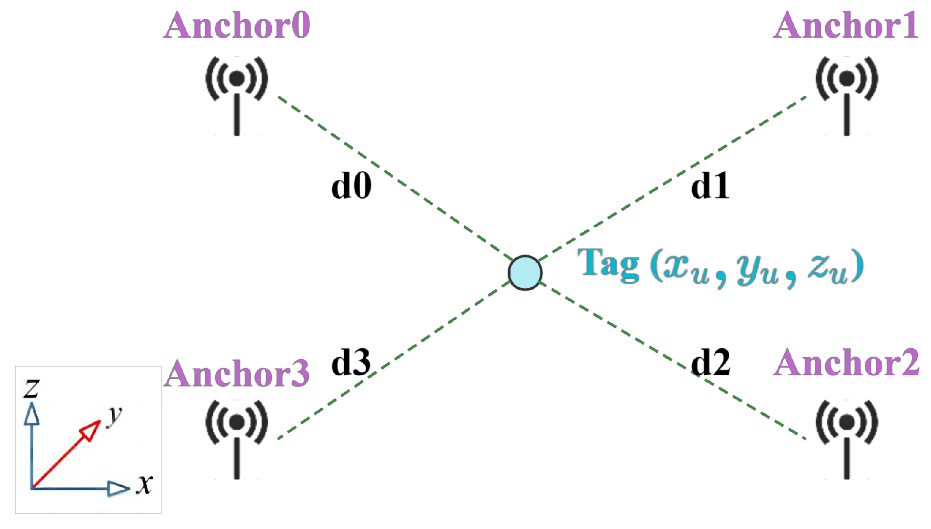
The UWB positioning system used in this work includes four stations at the corners and a tag on the mobile robot (Figure 1). To reduce interference and obstruction, the stations are elevated 2 m above ground on tripods. We denote as the label of the anchor station, where , and in this experiment. The coordinates of the four base stations are , , , and .
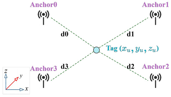
Figure 1.
Positional relationship between the anchors and the tag.
3.2. UWB Ranging Principle
The procedure for acquiring the three-dimensional coordinates of the tag sensor generally involves two main stages: (1) Utilizing the time-of-flight (TOF) ranging method to determine the distance between the tag and anchors [22], and (2) calculating the tag’s coordinates using the trilateration method with the least squares optimization algorithm.
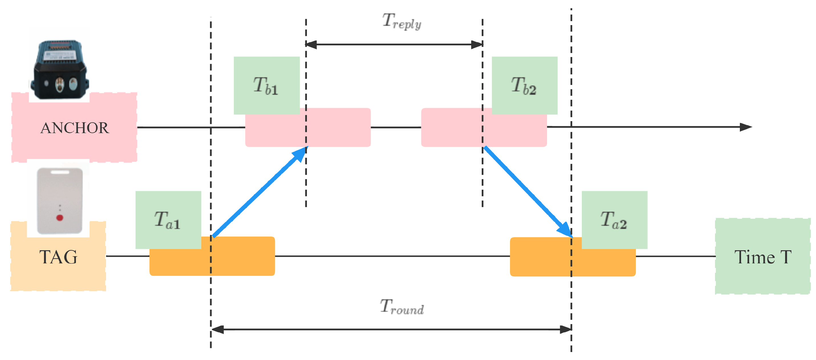
The ranging method used in this paper is TWR, and its ranging principle is shown in Figure 2. transmits a requested pulse signal to on its timestamp , then receives a signal at its own timestamp . return transmits a response signal to at a time , and receives the signal at a time . The distance D between the two modules can be calculated using Equation (1), which takes into account the propagation time of the pulse signal between the modules and where C represents the speed of light [23]. Figure 2 shows the positioning relationship of the anchors and the tag.
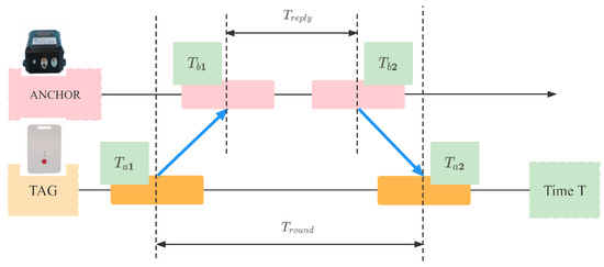
Figure 2.
TWR ranging principle.
We assume is the time interval between tags that transmit a signal and receive a return. represents the delay of each module [24]. The distance formula for the relationship between anchors and tags can be expressed as follows:
The trilateration algorithm (residual function) can be represented as Equation (3), which is the method used to establish a series of equations for position estimation, and we want to find its minimum. It should be a non-linear function:
is the first derivative of with respect to the tag coordinates . is the second derivative, and ignoring the higher-order derivative components, we can obtain:
where
Solving the matrix is challenging for large problems, so it’s usually avoided. For least-squares problems, practical methods include (1) ordinary least squares (OLS), (2) the Gaussian-Newton method, and (3) the Levenberg-Marquardt method [25].
3.3. Algorithm Selection
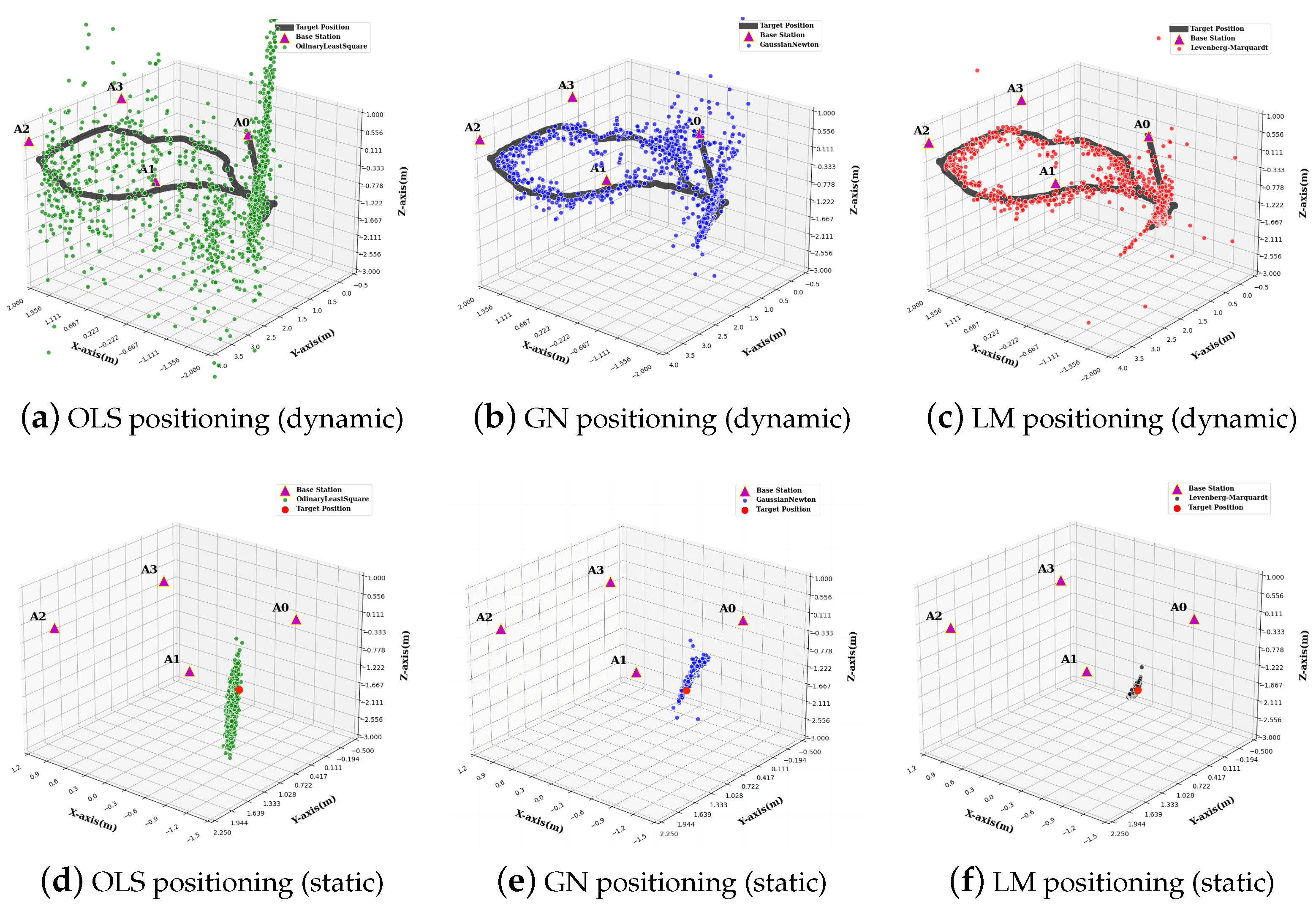
The OLS method estimates a mobile device’s location based on distances to fixed anchor points. Figure 3a,d shows the static and dynamic results. Figure 3a indicates high precision in horizontal (x and y) coordinates but less accuracy in vertical positioning.
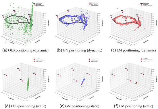
Figure 3.
Trajectories of the three methods: OLS (green), GN (blue), LM (red).
Gaussian-Newton’s method is a widely used optimization algorithm that employs a first-order Taylor expansion for faster convergence in non-linear problems. To minimize in the UWB trilateration method, we solve the following least squares problem:
By taking the derivative of the aforementioned equation concerning and expanding the square term of the objective function, we obtain the following equation after transformation.
Equation (9) is a system of linear equations for the variable , solved by the Gaussian-Newton or regular equation. We define the coefficients as H (left side) and g (right side). Figure 3b,e shows the dynamic and static positioning results.
For instance, during the actual positioning process, may be a positive semi-definite matrix, resulting in no solution for the equation. Another issue is that the approximation result may not be accurate enough if the resulting is too large. The Levenberg–Marquardt algorithm (LM) [25] addresses two issues encountered in the Gaussian–Newton method by introducing damping coefficients to the optimization process.
3.4. LM Parameters Setting
The main effect of LM is determined by the variation of , which is dependent on the fit’s accuracy as described by . And is a second-order Taylor expansion for error function . The following setting shows parameter changed for each iteration. The dynamic and static positioning results are shown in Figure 3c,f, respectively.
If :
Else:
3.5. Analysis of Results
The results of the ranging error analysis for the three methods, ordinary least squares (OLS), Gaussian–Newton (GN), and Levenberg–Marquardt (LM), are presented in Table 1.

Table 1.
LOS/NLOS positioning accuracy evaluation of the OLS, GN, LM methods.
In the LOS scenarios, the ranging errors for the three methods along the x-y plane were found to be similar, with error ranges between 0.157 m and −0.157 m and root mean square errors (RMSEs) at the centimeter level. This level of error is considered acceptable as it has a negligible impact on subsequent filtering and fusion processes.
However, compared with the error in the x-y plane, the RMSE values of the z-axis are significantly greater. For example, the RMSE for the OLS method in the LOS scenario was 0.638 m, while the GN method was 0.1328 m. The LM method is the best among the three and achieved a much smaller RMSE of 0.0905 m. One of the main reasons causing a larger error in the z-axis is due to the hardware configuration, where four anchors lie on the same plane. To improve the accuracy on the z-axis, adding more anchors can provide height variations among anchors.
In the NLOS scenarios, ranging errors are significantly larger than in the LOS, with obstacles causing decimeter-level errors. RMSE values rise to 11.8 cm and 15.7 cm for the LM method in the x-y plane, and 61.7 cm for the z-axis. The OLS and GN methods behave similarly, with errors 3–5 times bigger than in LOS scenarios.
In terms of positioning in NLOS conditions, all three methods perform poorly, with position RMSE values of 1.706 m, 0.886 m, and 0.74 m for OLS, GN, and LM, respectively. Although the LM method performs the best, it still does not achieve an acceptable level of accuracy. However, compared to the second-best GN method, the LM method shows a significant improvement in positioning accuracy, with RMSE errors reduced by 34.24% and 16.48% in LOS and NLOS, respectively.
4. Data Fusion Strategy
UWB system measurements are prone to errors from factors like multi-path effects and NLOS [26], leading to inaccurate indoor vehicle positioning. IMU-based technology offers low-cost, independent posture sensing but suffers from divergence due to sensor errors [27]. Meanwhile, binocular visual odometry provides six-degrees-of-freedom movement but accumulates positioning errors over time [28].
To address these limitations, this study proposes integrating UWB, IMU, and binocular visual odometry [29]. This fusion allows UWB to correct the cumulative errors of IMU/visual odometry, while the latter two smooth UWB data and mitigate multi-path effects [30], offering a more accurate and reliable positioning solution for indoor mobile vehicles.
4.1. System Structure Design
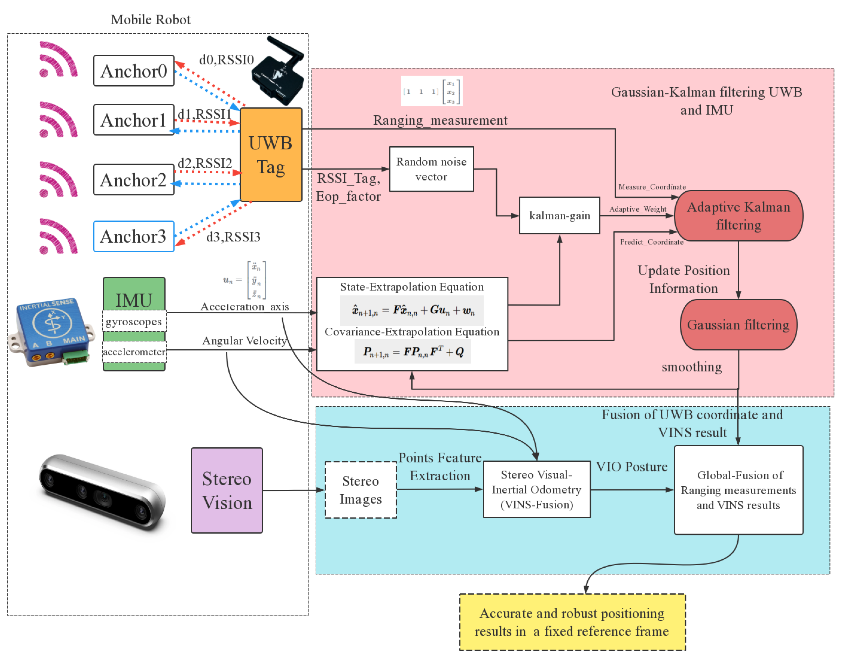
Figure 4 shows the system structure for fusing UWB/IMU with binocular VO data. The UWB system provides distance measurements , while the binocular VO [3] uses feature extraction, optical-flow matching, and reprojection for position and orientation, making it more complex. An adaptive Kalman filter first fuses UWB and IMU for stable, interference-resistant positioning. Then, graph optimization fuses the fixed UWB and visual odometry. This involves converting VIO-derived relative positions into global coordinates and using factor graph optimization (FGO) to tightly couple UWB and visual SLAM without loop closure.
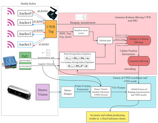
Figure 4.
The UWB/IMU and binocular VIO data fusion system structure designed.
4.2. Adaptive Kalman Filtering Model Design
Since we used the adaptive Kalman filter in this paper, the system state extrapolation equation is generally formed in matrix notation:
where is a predicted system state vector at time step n, is an estimated system state vector at the last time step . is a control variable, is the process noise, and the noise satisfies the Gaussian white noise. . F is the state transition matrix, and G is the control matrix. In this paper, we select to use a simplified state extrapolation equation:
The system state vector of the fusion system at time n is defined by:
denotes the x-axis position, is the x-axis velocity, and is the x-axis acceleration. The same notation applies to the y-axis and z-axis. The state transition matrix F can be defined as follows:
The represents the refresh rate of the filter. In this case, the UWB has a refresh rate of 50 Hz while the IMU has a refresh rate of 200 Hz, and a lower value, which is 0.02 s, is selected for in our experiments. The timestamps of the data from the two sensors are checked to ensure they are synchronized before being input into the filter algorithm. The covariance extrapolation equation is defined as follows:
is the prediction covariance matrix at timestamp n. It is generated by considering the covariance matrix from the last timestamp, . The Q matrix represents the process noise of the IMU (prediction noise).
Each component of the covariance extrapolation equation is a of two values. For example, represents the covariance of vector and vector .
The measurement equation for the fusion system is:
Let denote the observation vector of the fusion system at time n, and let H denote the observation matrix. The observation noise is denoted as , which is assumed to follow a Gaussian white noise distribution with . The observation vector at timestamp n is defined as the UWB coordinate measurement along with the velocity and acceleration measurements from IMU denoted as and , respectively. The observation matrix H is defined as an identity matrix with the diagonal elements being 1, i.e., :
represents the Kalman gain matrix, and (the update state) represents the optimal estimate of the state at time n. In the iterative process, the system noise covariance matrix and the observed noise covariance matrix are dynamically updated. The complete adaptive Kalman filter update process is as follows:
The state-update equation and covariance-update equation are shown below:
4.3. Channel Power Diagnostics Based on RSSI-EOP Factor
Identifying NLOS conditions using the complex impulse response (CIR) of UWB channels has been widely researched [31,32]. For this purpose, the references [31,33] examine CIR features. Reference [31] suggests a classifier to distinguish between LOS and NLOS conditions, while Reference [33] looks at the correlation between these features and ranging errors. A simpler method, recommended by Decawave [34], uses the ratio of energy in the timing pulse (first peak power level, or FPPL) to the overall RSSI to identify NLOS conditions. Those two diagnostics already allow for acceptable detection, as energy and the maximum amplitude of the received signal are significantly more attenuated in NLOS conditions [32]. Its simplicity and availability in Nooploop transducers make it popular.
Based on the experiment test results, we have determined the standard deviation of our IMU measurements to be approximately for acceleration. Consequently, we choose a value of for the diagonal elements of the noise covariance matrix .
In addition, we introduce a factor to incorporate the observation values and indicate the covariance frame to frame. The equation representing this relationship is provided below. The equation presented in the context combines five values, namely , , , , and , as recommended by our experiment design.
The estimation of precision () refers to the influence of the geometric layout of the base station and the target point on the positioning accuracy at a specific time, denoted as axis(), where n denotes the timestamp of such an EOP, allows us to monitor the stability of the system over time. represents the total signal strength received, encompassing the overall signal strength received from all directions. On the other hand, specifically denotes the signal strength of the first path, referring to the strength of the initial signal that arrives at the receiver.
The parameter serves as an empirical threshold value used to differentiate between LOS and NLOS conditions. In our experiments, we considered to be indicative of NLOS situations, although this value may be subject to adjustment.
The parameter is a scale factor employed to control the confidence interval of each axis. The propagation loss factor n is usually set to (LOS propagation), on the other hand, d represents the distance between the unknown tag and the anchor, while (in our hypothesis testing), denotes the fixed distance between the reference node and the anchor. If the channel is not purely LOS, the value of propagation losses and n has to change, accounting for the NLOS/multi-path effect.
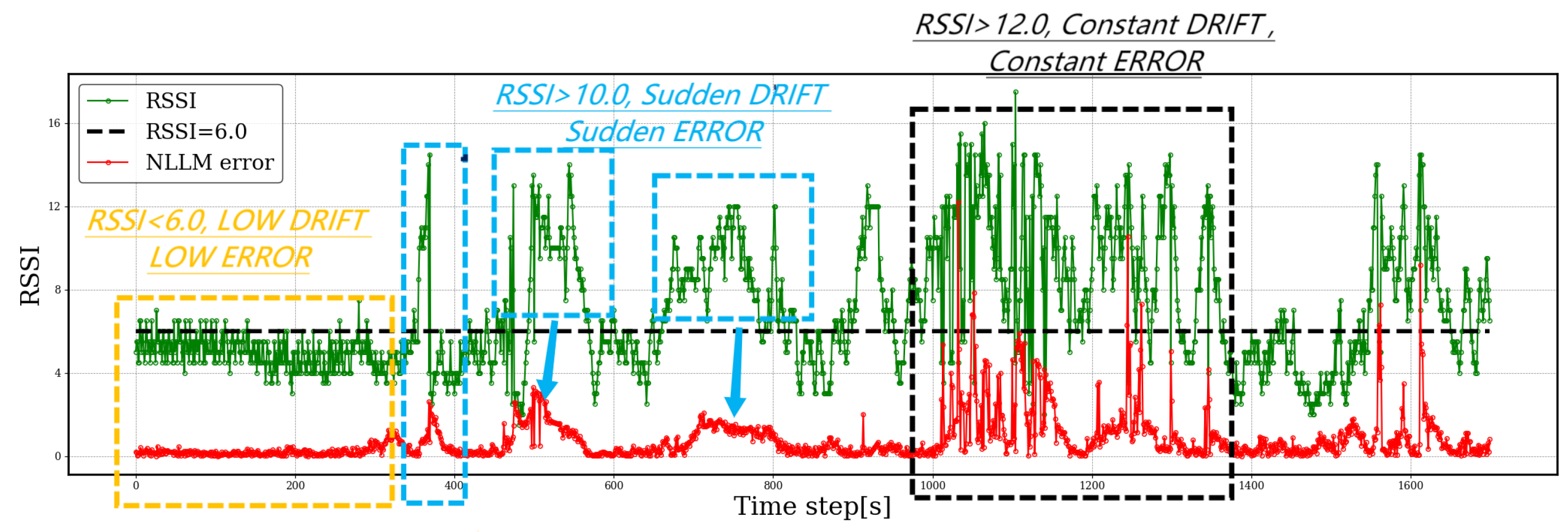
In this paper, we specifically utilize the RSSI-EOP metrics. For us to find a strong relationship between these two diagnostics, just as shown in Figure 5, the green color denotes the RSSI measurement from anchors, while the red line depicts the LM measurement error compared with the ground truth. Additionally, the black line indicates an empirical threshold (LOS/NLOS), denoted as . We noticed that the RSSI and LM errors exhibit similar trends. When the RSSI is below 6.0 dB, there is a low drift and low error, as evidenced by the absence of fluctuations in the red line. However, when the RSSI value exceeds 10.0 dB, which indicates the presence of NLOS data, sudden signal drifts occur, leading to multi-path effects and abrupt errors. Furthermore, when the RSSI surpasses 12.0 dB, it denotes prolonged heavy shading, causing persistent drift and constant errors.
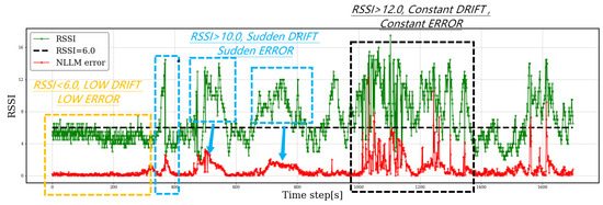
Figure 5.
Time series of the RSSI value (green) and the NLLM method error (red).
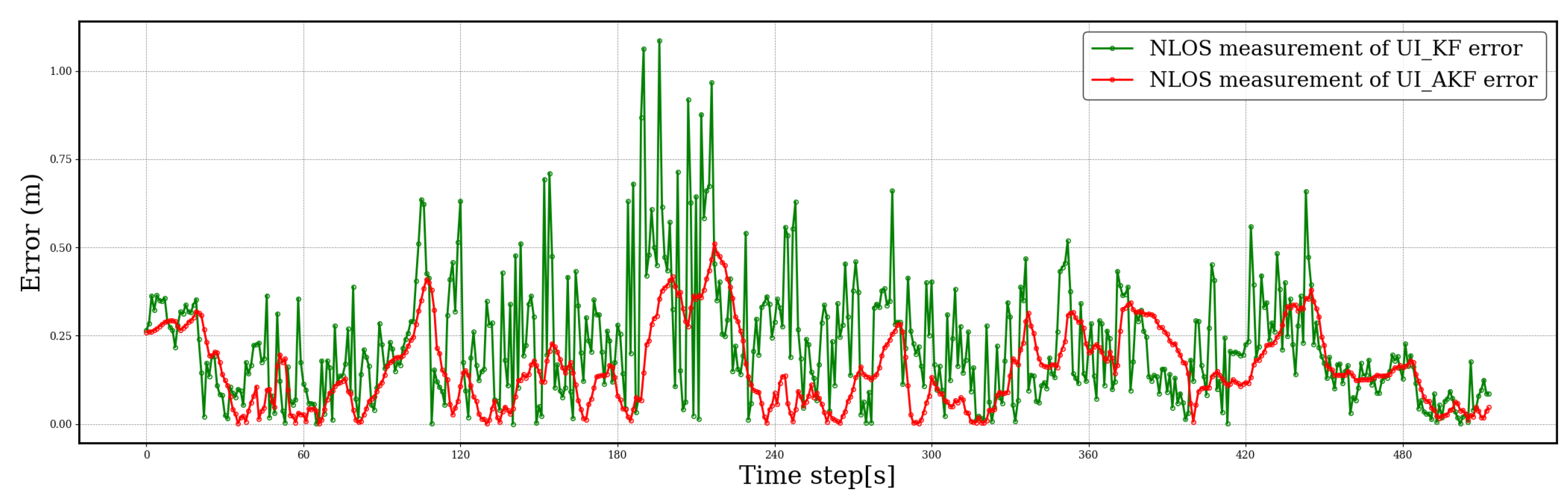
Figure 6 compares errors between two approaches: UI-KF (green) without RSSI feedback and UI-AKF (red) with RSSI feedback. The red line (UI-AKF) shows less fluctuation, indicating that adding RSSI feedback improves error performance in localization. This highlights the correlation between RSSI measurements and LM error, underscoring the importance of RSSI in enhancing localization accuracy.
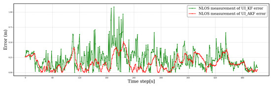
Figure 6.
Error measurements for the UI-KF (green/no feedback) and UI-AKF (red/RSSI feedback).
4.4. Experimental Study and Analysis of Results
Hardware Setup and Experiment Scene
The experiment’s hardware platform is a four-Mechanum-wheel KUKA youBot, as shown in Figure 7a. The robot connects to an NVIDIA Jetson Xavier for control, which boasts an eight-core ARMv8.2 64-bit CPU and an NVIDIA Volta GPU with 512 cores. The experiment utilizes the LinkTracK P-B module (Nooploop) as the UWB system, which offers a theoretical positioning accuracy of 15 cm and a communication range of up to 500 m. WHEELTEC (N-100N) provides the IMU, which guarantees a gyro bias within 0.05° RMS in static conditions and 0.1° RMS in dynamic conditions. The Realsense D455 camera, developed by Intel, captures binocular RGB images and computes depth information up to 10 m. It also uses a 16-line LiDAR (Helios-16) and the LINS method [35] to achieve accurate localization down to the centimeter level, providing ground-truth data. We set up ROS to facilitate seamless communication between various components.
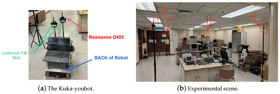
Figure 7.
Remote platform and experiment scene.
As shown in Figure 7b, the robot was commanded to navigate in a rectangular path along the aisles of an indoor environment, where the fixed furniture could lead to a multi-path or NLOS effect. The environment’s size is approximately 8.5 m by 4.9 m, and four anchors (A0–A3) are needed in this experiment. For the LOS scene, our route begins and ends at anchor 0, and for the NLOS scene, it starts and ends at anchor 2.
4.5. Analysis of Results
We can see that the Levenberg–Marquardt method has the best performance. Moreover, an NLOS-correction method shown in Algorithm 1 was adopted, and a threshold was demonstrated to filter out outliers. So, an NLOS-corrected LM method (NLLM) was used to compare with the adaptive Kalman filtering of IMU/UWB (UIAKF) and no adaptive version (UIKF).
| Algorithm 1: Outlier Detection |
Require: Outlier threshold
|
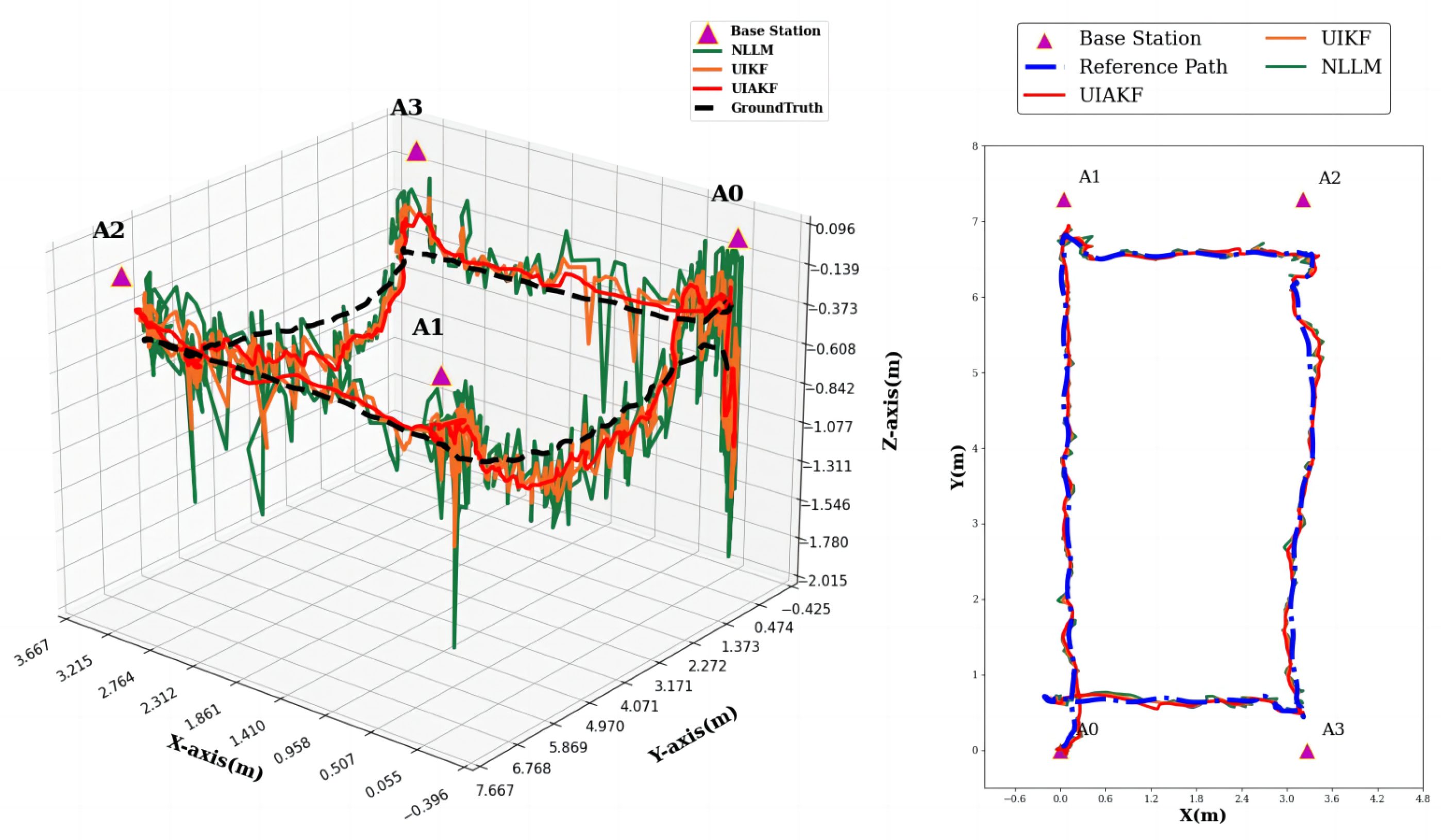
Figure 8 provides a comparison between the UIAKF, UIKF, NLLM, and reference paths. The red line represents the UIAKF path, the orange line represents UIKF, the green line represents NLLM, and the black line represents the reference path. The NLLM method struggles when faced with poor distance measurements in NLOS situations. If one of the anchors is blocked, the NLLM method can be negatively affected by such measurements, leading to issues like gradient explosions or outliers. As a result, the NLLM positioning errors fluctuate compared to the actual path.

Figure 8.
Comparison between NLLM/UIAKF and ground truth (LOS scene).
The UIAKF algorithm, utilizing an adaptive Kalman filter, outperforms the other methods in positioning accuracy and UWB path smoothness. The UIKF method ranks between UIAKF and NLLM in performance. While UIKF smooths changes using IMU data, it doesn’t assess UWB distance measurement quality via the RSSI-EOP factor, assigning fixed confidence to measurements. This can lead to unpredictable outcomes and high confidence in inaccurate measurements.
Figure 8 compares NLLM, UIAKF, UIKF, and reference paths in the X-Y plane, showing small positioning errors and good performance in LOS scenarios.
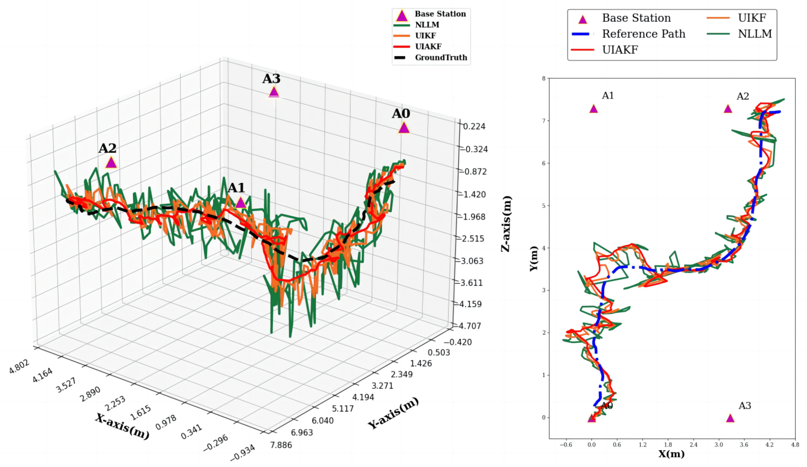
In the second test, the KUKA robot followed a Z-shaped curve in an NLOS environment (Figure 9). The UWB tag was placed at a lower height, leading to increased interference and poor distance measurements. This test aimed to demonstrate that the UIAKF algorithm achieves better-ranging accuracy in challenging environments.
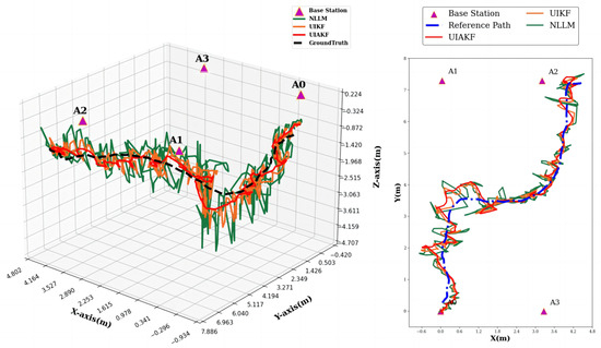
Figure 9.
Comparison between NLLM/UIAKF and ground truth (NLOS scene).
In summary, the UIAKF method outperforms UWB-only positioning, offering a smoother UWB path. The UIKF method performs between UIAKF and NLLM, while NLLM struggles with NLOS scenarios, showing fluctuating positioning errors.
The second test scene had a more significant negative impact, with more outliers in both the Z and X-Y planes compared to the first test. However, the UIAKF and UIKF algorithms mitigated some NLOS errors using the motion extrapolation equation (predict function) that relies on IMU data for position estimation. Additionally, a special gain parameter G, influenced by , , , and , controls the UWB noise covariance, with a higher G indicating more reliable motion estimation.
The results show that the proposed UWB/IMU Kalman fusion system closely approximates the actual path, smooths the UWB driving path, and reduces NLOS-induced errors compared to the NLLM algorithm.
The ranging error analysis results for the NLLM, UIKF, and UIAKF methods are presented in Table 2. In LOS scenarios, the ranging errors in the x-y axis were found to be similar for all three methods, with error ranges between −0.080 m and 0.055 m and RMSE at the centimeter level. This error level is considered acceptable and has a negligible impact on subsequent filtering and fusion processes. As expected, the error in the z-axis is higher than the other two axes due to the hardware setting. For the z-axis, the NLLM method exhibited the largest RMSE value of 0.265 m. In contrast, the UIKF and UIAKF methods achieved a smaller RMSE value of 0.1546 m and 0.185 m, respectively.
Table 2.
LOS/NLOS positioning accuracy evaluation of the OLS, GN, LM methods.
In NLOS scenarios, x-y axis ranging errors were about three times larger than in LOS scenes. The UIAKF method’s RMSE increased to 21.3 cm (x-axis) and 17.7 cm (y-axis), with similar trends in the UIKF and NLLM methods. On the z-axis, the NLLM method had poor performance with a 44.6 cm RMSE, while the UIAKF and UIKF methods performed better, with RMSEs under 30 cm—0.466 m, 0.193 m, and 0.284 m, respectively.
An availability of ±0.2 m is used to indicate the performance of 3D positioning using different methods. As shown in the Table, the proposed UIAKF method achieved the highest availability among the three, with 75.917% and 40.645% of data falling within ± 0.2 m Euclidean distance error.
These results highlight the improvement of the proposed fusion scheme, UIAKF, in reducing position errors in both LOS and NLOS scenarios, offering a more accurate method for position evaluation in a mixed environment.
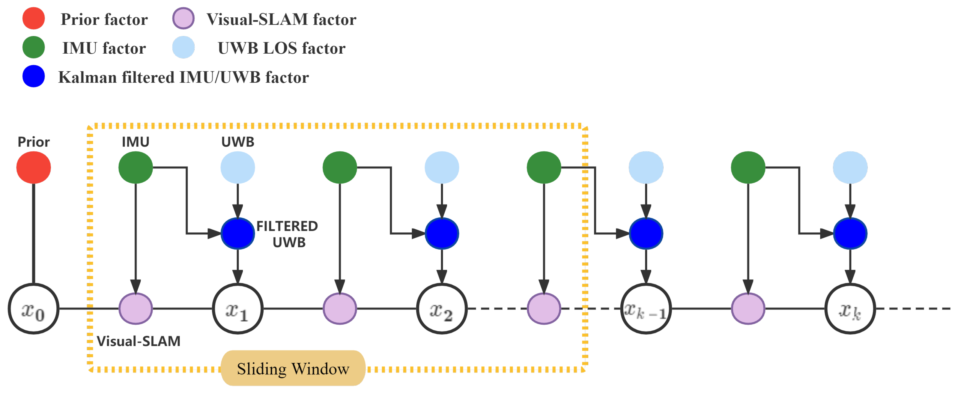
5. UWB/IMU-Visual SLAM Integrated Model Based on Factor Graph Optimization
In the context of the FGO-based UWB/IMU-visual SLAM integrated system, shown in Figure 10, both UWB-IMU Kalman fusion results and visual-inertia odometry (VIO) are coupled using factor graph optimization (FGO). The system’s navigation states are represented by variable nodes (hollow circles), while prior information is depicted by a solid red circle. The visual-SLAM component is represented by a purple circle, the original UWB measurements by light blue circles, and the IMU factor by a green circle.

Figure 10.
Framework of the FGO-based UWB/IMU and visual-SLAM tightly coupled integrated system.
The visual-SLAM state between two consecutive frames is a local constraint; it defines the relative pose between two nodes, essentially constraining the estimated motion from one node to another. Additional nodes represent global constraints originating from global (UWB) sensors.
Both the UWB fusion system and VIO receive the IMU information at the same timestamps, enabling a flexible combination of sensor information with various measurement frequencies. Normally, visual sensors have the lowest frequency (20–30 Hz), which is used to determine the node frequency. This study employs the sliding window method, which sets the number of historical variables used for computation. The size is empirically tuned through experiments to ensure the output rate matches the refresh rate from the visual sensor.
5.1. Factor Graph Optimization Model
The goal of multi-sensor data fusion is to estimate the system’s optimal posterior state based on sensor measurements. Naturally, we can transform the optimal posterior state into a maximum likelihood estimation (MLE) problem and solve it. This study definitively includes UWB, IMU, and visual-SLAM measurements. It is firmly assumed that the UWB-IMU fusion and visual-inertial odometry (VIO) systems are completely independent of each other. We can formulate the MLE problem of the UWB/IMU/camera integrated system as follows:
where represents the global pose nodes, , where and denote the position and orientation between the VIO-frame (local) and UWB-frame (global). S denotes the measurement queues, which include local measurements (VIO) and global measurements (UWB) [5]. For our assumption, the noise of measurements follows a Gaussian distribution with mean and covariance, which is denoted as , Thus, we derive the aforementioned equation as follows:
In an FGO-based integrated model, the sensor measurements are thought of as factors that are connected to the state x. Each of these factors has an error function that needs to be minimized, and can be related to the error function for both the measurement and the projection. The error function associated with a measurement and reprojection can be defined as the difference between the predicted measurement and the actual measurement. Let us denote the predicted measurement as and the actual measurement as z. We can then express the error function as follows:
Here, signifies the covariance matrix of the observation process, where the uncertainties of the ultra-wideband (UWB) and visual-SLAM systems are determined based on the ranging accuracy and the degree of matching, respectively. Additionally, represents the Euclidean norm of the vector. Taking the negative logarithm of Equation (27) and discarding the coefficient terms, the MLE problem can be transformed into a non-linear least squares (NLS) problem:
The superscripts and are used to denote the number of UWB measurement residuals and visual-SLAM measurement residuals, respectively. The superscript n represents the number of UWB anchors. The subscripts j and k indicate the indexes of UWB factors and visual-SLAM factors in the factor graph. The subscript i corresponds to the index of UWB anchors. The notation represents the UWB anchor coordinates. The term denotes the measurement residuals associated with the UWB sensor, specifically the residuals of ranging. Furthermore, and denote the measurement residuals associated with the visual sensor, specifically the residuals of translation and rotation. We can express the error functions associated with UWB and visual-SLAM factors as follows:
The symbol ⊗ represents the multiplication operator of the quaternion. The term represents the AKF-filtered IMU-UWB measurements, while and represent the actual visual-SLAM measurements.
By minimizing the objective function stated above, the maximum posterior solution for the set of states can be obtained. Recognizing that the computational load increases significantly as the scale of the factor graph grows due to the continuous addition of new measurement information over time, this study employs a sliding window method. This method ensures the relative stability of the number of optimized variables by discarding the earliest historical variables in the window.
5.2. Evaluation of the UWB/IMU/Visual-SLAM Integrated Positioning Algorithm
To evaluate the effectiveness of the proposed NLOS correction method using the adaptive prediction model (UIAKF), NLLM, and visual-odometry-SLAM (VINS-Fusion [5]), no adaptive FGO-based VINS-Fusion + UIKF, FGO-based VINS-Fusion + UIAKF are all variously used as the inputs to the positioning method, and the methods mentioned below are the abbreviations obtained for comparison:
- Levenberg–Marquardt method positioning + NLOS outlier correction (NLLM) (green);
- Levenberg–Marquardt method positioning + NLOS outlier correction + adaptive Kalman filtering of IMU (UIAKF) (orange);
- Visual-IMU odometry (VINS-Fusion) (black);
- FGO-Based VINS-Fusion + UIKF Fusion (UIKF-VINS-FGO) (yellow);
- FGO-Based VINS-Fusion + UIAKF Fusion (UIAKF-VINS-FGO) (red);
- Ground truth (blue);
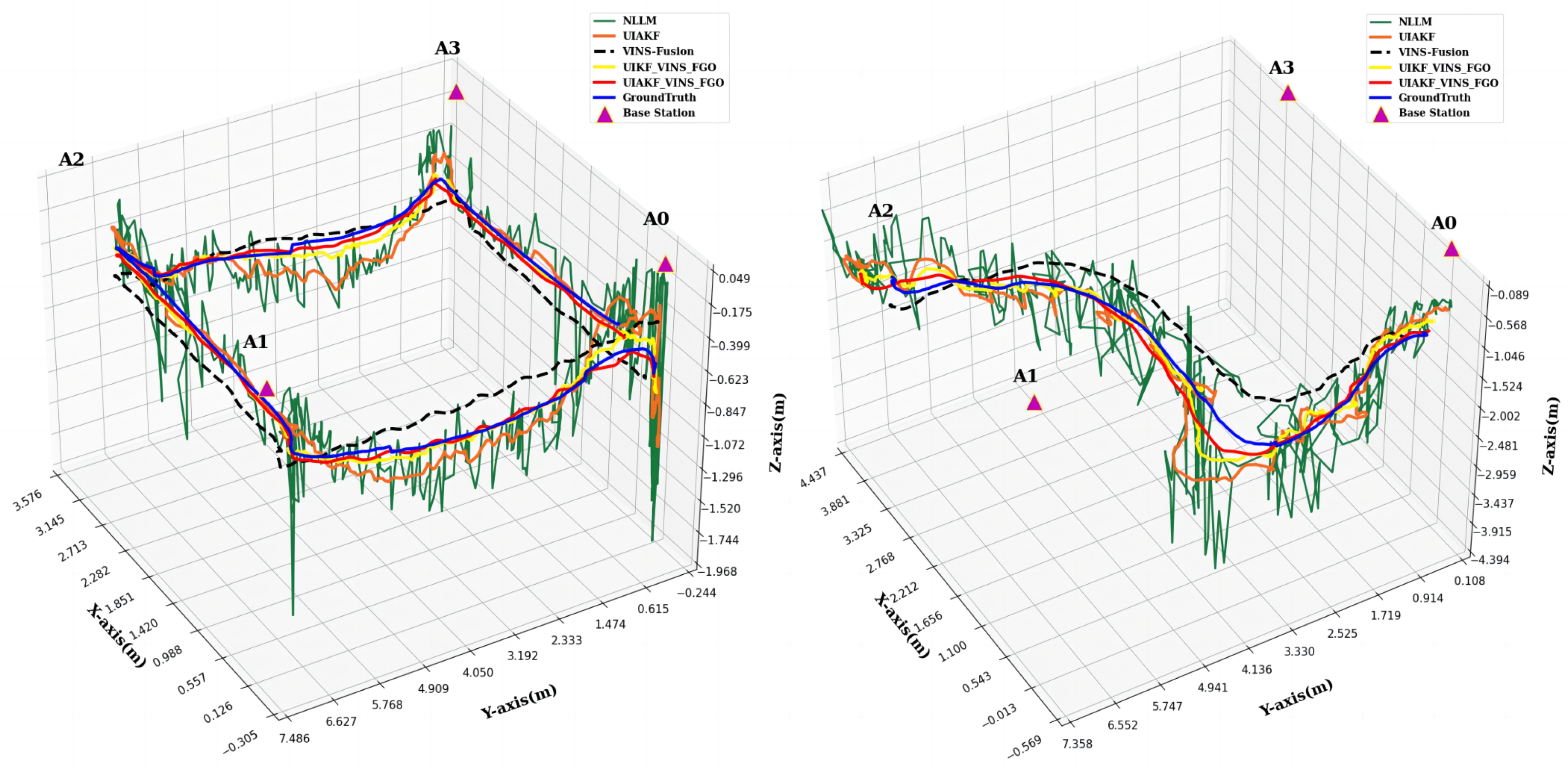
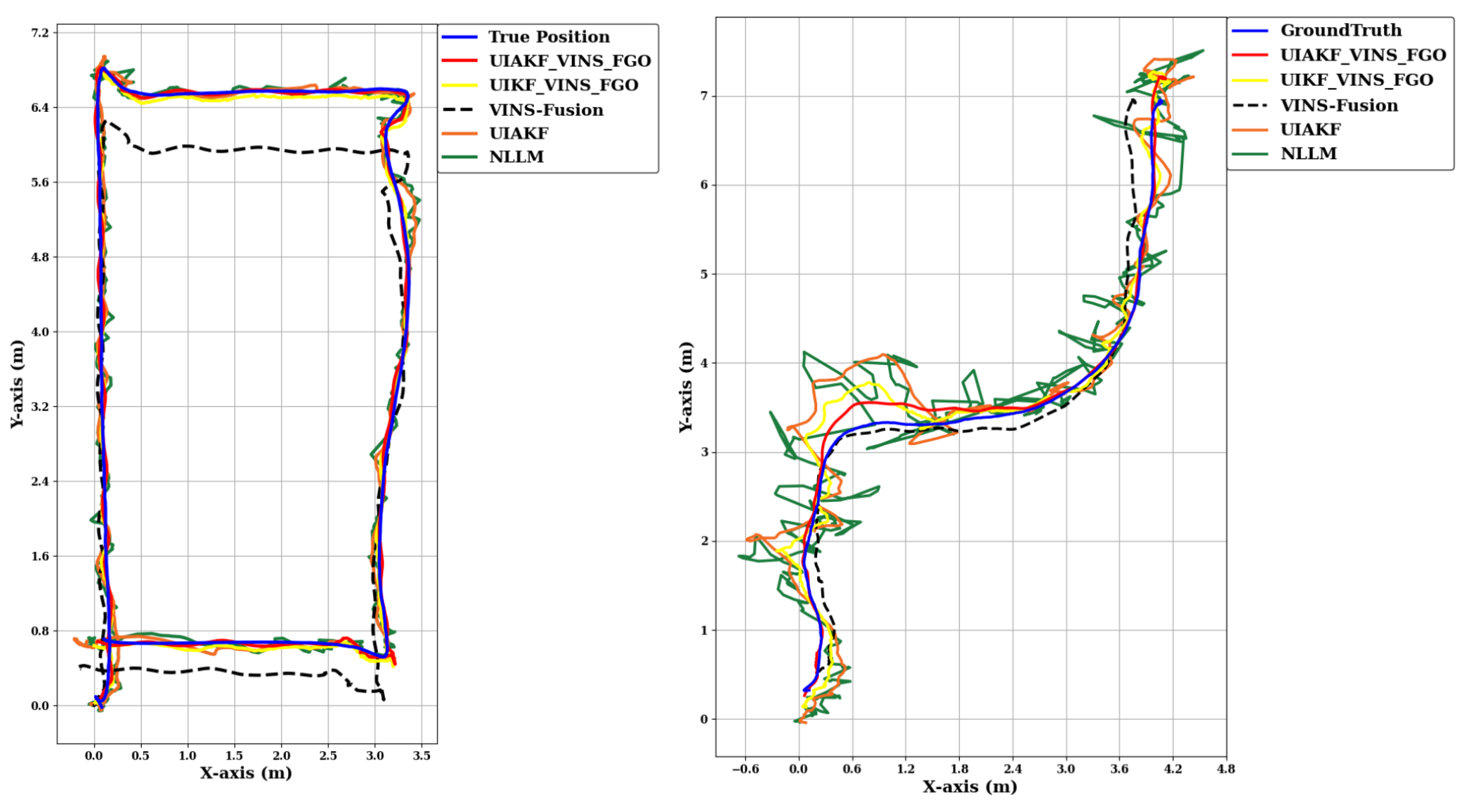
Figure 11 shows a comparison of the trajectories estimated using the different methods with the reference trajectory in 3D, and Figure 12 shows a comparison of the trajectories estimated using the different methods with the reference trajectory in 2D. Table 3 reports the positioning performance of each method.
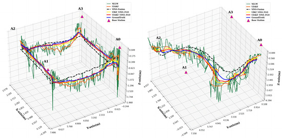
Figure 11.
LOS/NLOS trajectories of the five methods in 3D: NLLM (Green), UIAKF (Orange), VINS-Fusion (Black), UIKF-VINS-FGO (Yellow), UIAKF-VINS-FGO (Red), ground truth (Blue).
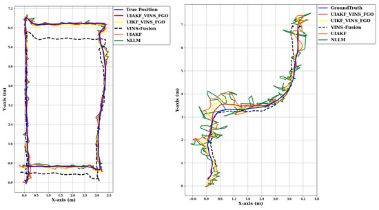
Figure 12.
LOS/NLOS trajectories of the five methods in 2D: NLLM (Green), UIAKF (Orange), VINS-Fusion (Black), UIKF-VINS-FGO (Yellow), UIAKF-VINS-FGO (Red), ground truth (Blue).
Table 3.
LOS/NLOS positioning accuracy evaluation of the LM, NLLM, UIKF, UIAKF, VINS, and UIAKF-VINS-FGO methods.
The results in Table 3 demonstrate that the UIAKF method outperforms the other three methods, which solely utilize UWB/UWB+IMU/VIO. The UIAKF method significantly improves the positioning performance of the integrated system by adjusting the measurement noise covariance matrix. This adjustment mitigates the impact of abnormal measurements on parameter estimation, particularly when NLOS or multi-path effects contaminate the direct input of UWB raw measurements. The UIAKF method achieves a reduction in RMSEs compared to NLLM of 17.33% in the X direction, 8.19% in the Y direction, and 31.8% in the plane direction.
Furthermore, despite the dissimilarities in methodology and error characteristics between VINS-Fusion and UIAKF, with VINS primarily affected by accumulated errors and UIAKF influenced by fluctuating standard deviation errors concerning the ground truth, the UIAKF method exhibits similar initial performance to VINS-Fusion but outperforms it in the long run. Notably, VINS demonstrates good performance initially but gradually deteriorates due to the increasing deviation between its estimated position and the ground truth. VINS relies on camera SLAM estimation instead of absolute calculations based on observation data. In comparison to VINS-Fusion, UIAKF achieves reductions in RMSEs of 6.9% in the X direction, 68.2% in the Y direction, and 65.8% in the z direction.
However, when employing the FGO method (UIAKF-VINS-FGO), which assigns equal weights to measurements of varying qualities, the positioning accuracy is better than single or dual sensor approaches (VINS-Fusion or UIAKF methods). Even compared to the non-adaptive version (UIKF-VINS-FGO), both algorithms perform excellently in LOS scenes, with errors below 10 cm for all three axes. UIAKF-VINS-FGO shows a clear advantage in NLOS scenes, achieving RMSE reductions of 37.09% in the X direction, 31.9% in the Y direction, and 19.08% in the Z direction. Additionally, using a threshold of ±0.2 m to define availability based on the temporal correlation between measurements and redundant system measurements. It achieves 100% availability, indicating all measurement errors are below the threshold, significantly outperforming the UIKF_VINS_FGO (91.17%), UIAKF methods (77.02%) and VINS-Fusion (52.033%). Even in the NLOS scene, UIAKF-VINS-FGO maintains the highest performance with an availability of 89.2%, compared to 73.37% for UIKF_VINS_FGO, 42.21% for UIAKF, and 57.02% for VINS-Fusion.
The proposed method (UIAKF-VINS-FGO) clearly achieves the best results in both the adaptive Kalman filtering-based integrated framework and the FGO-based integrated framework when comparing the five integrated positioning methods that combine UWB/IMU and visual SLAM. This method utilizes AKF-filtered UWB+IMU localization signals as input, particularly AKF’s dynamic adjustment of the weight of NLOS/LOS measurements in integrated systems, significantly enhancing the positioning performance of the UWB/IMU systems, and proposes an NLOS identification and correction to minimize outliers. Finally, the integrated system employs FGO-based fusion with VIO. These findings provide valuable insights for researchers and practitioners aiming to improve the accuracy of integrated positioning solutions.
6. Conclusions
An integrated UWB/IMU visual SLAM system offers an effective solution for precise positioning in GNSS-denied environments. However, UWB NLOS errors can significantly impact the accuracy and effectiveness of the integrated system. We employ several key strategies to address this challenge and improve fusion performance.
Firstly, the study focuses on comparing RSSI and EOP factors for UWB NLOS identification and exclusion, ensuring stringent control over the data quality of system inputs. This helps in effectively managing the influence of NLOS errors on the integrated system.
Secondly, the calculated NLOS factor, denoted as , is incorporated into the Levenberg–Marquardt method. The confidence level of each anchor distance error function is adjusted accordingly. This step aids in refining the measurements and contributes to more accurate positioning results.
Furthermore, we propose an NLOS correction method using the AKF model for areas with poor shading. The calculated NLOS factor also modifies the measurement covariance matrix, directly influencing the adjustment of the Kalman gain matrix. By increasing the number of measurements, the integrated system maintains high accuracy and robustness.
Lastly, FGO-based UWB/IMU and visual SLAM integrated systems are designed. Dynamic positioning experiments were conducted to evaluate the system’s performance. The results demonstrate the effectiveness of the proposed methods.
The corrected measurements constructed using the Levenberg–Marquardt method outperform OLS and GN with a single sensor. The UIKF/UIAKF methods, which utilize dual sensors (UWB and IMU) and incorporate the corrected measurements, achieve satisfactory results. The RMSE in the plane direction is reduced to 0.185 m and 0.1546 m, respectively. The availability of errors below 0.2 m reaches 68.58% and 77.02% in LOS scenarios. Even in NLOS scenarios, these methods show a 10–26% improvement compared to a single UWB sensor (NLLM). This validates the effectiveness of the proposed NLOS correction method and the AKF model.
The UIAKF-VINS-FGO method, which leverages both the AKF-based model and the FGO-based model, outperforms using either model individually. This approach achieves optimal positioning accuracy and robustness, with RMSEs of 0.0224 m, 0.0218 m, and 0.0192 m in the X, Y, and plane directions for LOS scenarios and 0.095 m, 0.1178 m, and 0.2112 m for NLOS scenarios. The method demonstrates 100% availability in LOS scenarios and 89.2% availability overall, highlighting its superiority.
Future work will focus on integrating the existing system with point cloud or image feedback. This will help detect obstacles and shaded areas, enabling the system to adapt and enhance the accuracy and robustness of the positioning system in highly dynamic and degrading environments. The incorporation of RSSI and EOP factors, which are not always sensitive or responsive, will further contribute to system performance improvements.
Author Contributions
Conceptualization, J.L. and H.K.C.; methodology, J.L.; software, J.L. and S.W.; formal analysis, J.L. and S.W.; data collection, J.L., B.M. and J.H.; writing—original draft preparation, J.L. and S.W.; writing—review and editing, J.L., S.W. and H.K.C.; supervision, H.K.C.; funding acquisition, H.K.C. All authors have read and agreed to the published version of the manuscript.
Funding
This research was supported in part by the project P23-0089 of the Hong Polytechnic University, and the project ECF120/2021 of the Environment and Conservation Fund.
Data Availability Statement
No new data were created or analyzed in this study. Data sharing is not applicable to this article.
Conflicts of Interest
The authors declare no conflict of interest.
References
- Mur-Artal, R.; Tardós, J.D. ORB-SLAM2: An Open-Source SLAM System for Monocular, Stereo, and RGB-D Cameras. IEEE Trans. Robot. 2017, 33, 1255–1262. [Google Scholar] [CrossRef]
- Geneva, P.; Eckenhoff, K.; Lee, W.; Yang, Y.; Huang, G. OpenVINS: A Research Platform for Visual-Inertial Estimation. In Proceedings of the 2020 IEEE International Conference on Robotics and Automation (ICRA), Paris, France, 31 May–31 August 2020; pp. 4666–4672. [Google Scholar] [CrossRef]
- Qin, T.; Li, P.; Shen, S. VINS-Mono: A Robust and Versatile Monocular Visual-Inertial State Estimator. IEEE Trans. Robot. 2018, 34, 1004–1020. [Google Scholar] [CrossRef]
- Zhuang, Y.; El-Sheimy, N. Tightly-Coupled Integration of WiFi and MEMS Sensors on Handheld Devices for Indoor Pedestrian Navigation. IEEE Sens. J. 2016, 16, 224–234. [Google Scholar] [CrossRef]
- Qin, T.; Cao, S.; Pan, J.; Shen, S. A General Optimization-based Framework for Global Pose Estimation with Multiple Sensors. arXiv 2019, arXiv:1901.03642. [Google Scholar]
- Gomez-Ojeda, R.; Moreno, F.A.; Zuñiga-Noël, D.; Scaramuzza, D.; Gonzalez-Jimenez, J. PL-SLAM: A Stereo SLAM System Through the Combination of Points and Line Segments. IEEE Trans. Robot. 2019, 35, 734–746. [Google Scholar] [CrossRef]
- Li, S.; Hedley, M.; Bengston, K.; Humphrey, D.; Johnson, M.; Ni, W. Passive Localization of Standard WiFi Devices. IEEE Syst. J. 2019, 13, 3929–3932. [Google Scholar] [CrossRef]
- Hu, S.; He, K.; Yang, X.; Peng, S. Bluetooth Fingerprint based Indoor Localization using Bi-LSTM. In Proceedings of the 2022 31st Wireless and Optical Communications Conference (WOCC), Shenzhen, China, 11–12 August 2022; pp. 161–165. [Google Scholar] [CrossRef]
- Watthanawisuth, N.; Tuantranont, A.; Kerdcharoen, T. Design of mobile robot for real world application in path planning using ZigBee localization. In Proceedings of the 2014 14th International Conference on Control, Automation and Systems (ICCAS 2014), Gyeonggi-do, Republic of Korea, 22–25 October 2014; pp. 1600–1603. [Google Scholar] [CrossRef]
- Sun, W.; Xue, M.; Yu, H.; Tang, H.; Lin, A. Augmentation of Fingerprints for Indoor WiFi Localization Based on Gaussian Process Regression. IEEE Trans. Veh. Technol. 2018, 67, 10896–10905. [Google Scholar] [CrossRef]
- Zhang, M.; Jia, J.; Chen, J.; Deng, Y.; Wang, X.; Aghvami, A.H. Indoor Localization Fusing WiFi With Smartphone Inertial Sensors Using LSTM Networks. IEEE Internet Things J. 2021, 8, 13608–13623. [Google Scholar] [CrossRef]
- Silva, B.; Pang, Z.; Åkerberg, J.; Neander, J.; Hancke, G. Experimental study of UWB-based high precision localization for industrial applications. In Proceedings of the 2014 IEEE International Conference on Ultra-WideBand (ICUWB), Paris, France, 1–3 September 2014; pp. 280–285. [Google Scholar] [CrossRef]
- Chan, Y.; Ho, K. A simple and efficient estimator for hyperbolic location. IEEE Trans. Signal Process. 1994, 42, 1905–1915. [Google Scholar] [CrossRef]
- Liu, Y.; Zhu, X.; Bo, X.; Yang, Z.; Zhao, Z. Ultra-wideband high precision positioning system based on SDS-TWR algorithm. In Proceedings of the 2021 International Applied Computational Electromagnetics Society (ACES-China) Symposium, Chengdu, China, 28–31 July 2021; pp. 1–2. [Google Scholar] [CrossRef]
- Hol, J.D.; Dijkstra, F.; Luinge, H.; Schon, T.B. Tightly coupled UWB/IMU pose estimation. In Proceedings of the 2009 IEEE International Conference on Ultra-Wideband, Vancouver, BC, Canada, 9–11 September 2009; pp. 688–692. [Google Scholar] [CrossRef]
- Dwek, N.; Birem, M.; Geebelen, K.; Hostens, E.; Mishra, A.; Steckel, J.; Yudanto, R. Improving the Accuracy and Robustness of Ultra-Wideband Localization Through Sensor Fusion and Outlier Detection. IEEE Robot. Autom. Lett. 2020, 5, 32–39. [Google Scholar] [CrossRef]
- Wen, K.; Yu, K.; Li, Y.; Zhang, S.; Zhang, W. A New Quaternion Kalman Filter Based Foot-Mounted IMU and UWB Tightly-Coupled Method for Indoor Pedestrian Navigation. IEEE Trans. Veh. Technol. 2020, 69, 4340–4352. [Google Scholar] [CrossRef]
- Chen, Z.; Xu, A.; Sui, X.; Wang, C.; Wang, S.; Gao, J.; Shi, Z. Improved-UWB/LiDAR-SLAM Tightly Coupled Positioning System with NLOS Identification Using a LiDAR Point Cloud in GNSS-Denied Environments. Remote Sens. 2022, 14, 1380. [Google Scholar] [CrossRef]
- Zeng, Q.; Liu, D.; Lv, C. UWB/Binocular VO Fusion Algorithm Based on Adaptive Kalman Filter. Sensors 2019, 19, 4044. [Google Scholar] [CrossRef] [PubMed]
- Nguyen, T.H.; Nguyen, T.M.; Xie, L. Range-Focused Fusion of Camera-IMU-UWB for Accurate and Drift-Reduced Localization. IEEE Robot. Autom. Lett. 2021, 6, 1678–1685. [Google Scholar] [CrossRef]
- Yang, B.; Li, J.; Zhang, H. UVIP: Robust UWB aided Visual-Inertial Positioning System for Complex Indoor Environments. In Proceedings of the 2021 IEEE International Conference on Robotics and Automation (ICRA), Xi’an, China, 30 May–5 June 2021; pp. 5454–5460. [Google Scholar] [CrossRef]
- Ding, L.; Zhu, X.; Zhou, T.; Wang, Y.; Jie, Y.; Su, Y. Research on UWB-Based Indoor Ranging Positioning Technolog and a Method to Improve Accuracy. In Proceedings of the 2018 IEEE Region Ten Symposium (Tensymp), Sydney, NSW, Australia, 4–6 July 2018; pp. 69–73. [Google Scholar] [CrossRef]
- Mazraani, R.; Saez, M.; Govoni, L.; Knobloch, D. Experimental results of a combined TDOA/TOF technique for UWB based localization systems. In Proceedings of the 2017 IEEE International Conference on Communications Workshops (ICC Workshops), Paris, France, 21–25 May 2017; pp. 1043–1048. [Google Scholar] [CrossRef]
- Gu, Y.; Yang, B. Clock Compensation Two-Way Ranging (CC-TWR) Based on Ultra-Wideband Communication. In Proceedings of the 2018 Eighth International Conference on Instrumentation & Measurement, Computer, Communication and Control (IMCCC), Harbin, China, 19–21 July 2018; pp. 1145–1150. [Google Scholar] [CrossRef]
- Cheung, K.; So, H.; Ma, W.K.; Chan, Y. Least squares algorithms for time-of-arrival-based mobile location. IEEE Trans. Signal Process. 2004, 52, 1121–1130. [Google Scholar] [CrossRef]
- Malyavej, V.; Udomthanatheera, P. RSSI/IMU sensor fusion-based localization using unscented Kalman filter. In Proceedings of the The 20th Asia-Pacific Conference on Communication (APCC2014), Pattaya, Thailand, 1–3 October 2014; pp. 227–232. [Google Scholar] [CrossRef]
- Fakharian, A.; Gustafsson, T.; Mehrfam, M. Adaptive Kalman filtering based navigation: An IMU/GPS integration approach. In Proceedings of the 2011 International Conference on Networking, Sensing and Control, Delft, The Netherlands, 11–13 April 2011; pp. 181–185. [Google Scholar] [CrossRef]
- Tardif, J.P.; George, M.; Laverne, M.; Kelly, A.; Stentz, A. A new approach to vision-aided inertial navigation. In Proceedings of the 2010 IEEE/RSJ International Conference on Intelligent Robots and Systems, Taipei, Taiwan, 18–22 October 2010; pp. 4161–4168. [Google Scholar] [CrossRef]
- Lee, Y.; Lim, D. Vision/UWB/IMU sensor fusion based localization using an extended Kalman filter. In Proceedings of the 2019 IEEE Eurasia Conference on IOT, Communication and Engineering (ECICE), Yunlin, Taiwan, 3–6 October 2019; pp. 401–403. [Google Scholar] [CrossRef]
- Zhang, R.; Fu, D.; Chen, G.; Dong, L.; Wang, X.; Tian, M. Research on UWB-Based Data Fusion Positioning Method. In Proceedings of the 2022 28th International Conference on Mechatronics and Machine Vision in Practice (M2VIP), Nanjing, China, 16–18 November 2022; pp. 1–6. [Google Scholar] [CrossRef]
- Sabatelli, S.; Galgani, M.; Fanucci, L.; Rocchi, A. A double stage Kalman filter for sensor fusion and orientation tracking in 9D IMU. In Proceedings of the 2012 IEEE Sensors Applications Symposium Proceedings, Brescia, Italy, 7–9 February 2012; pp. 1–5. [Google Scholar] [CrossRef]
- Wymeersch, H.; Marano, S.; Gifford, W.M.; Win, M.Z. A Machine Learning Approach to Ranging Error Mitigation for UWB Localization. IEEE Trans. Commun. 2012, 60, 1719–1728. [Google Scholar] [CrossRef]
- Maranò, S.; Gifford, W.M.; Wymeersch, H.; Win, M.Z. NLOS identification and mitigation for localization based on UWB experimental data. IEEE J. Sel. Areas Commun. 2010, 28, 1026–1035. [Google Scholar] [CrossRef]
- Decawave. Dw1000 Metrics for Estimation of Non Line of Sight Operating Conditions; Technical Report aps013 Part 3 Application Note; Decawave: Dublin, Ireland, 2016. [Google Scholar]
- Qin, C.; Ye, H.; Pranata, C.E.; Han, J.; Zhang, S.; Liu, M. LINS: A Lidar-Inertial State Estimator for Robust and Efficient Navigation. In Proceedings of the 2020 IEEE International Conference on Robotics and Automation (ICRA), Paris, France, 31 May–31 August 2020; pp. 8899–8906. [Google Scholar] [CrossRef]

Disclaimer/Publisher’s Note: The statements, opinions and data contained in all publications are solely those of the individual author(s) and contributor(s) and not of MDPI and/or the editor(s). MDPI and/or the editor(s) disclaim responsibility for any injury to people or property resulting from any ideas, methods, instructions or products referred to in the content. |
© 2024 by the authors. Licensee MDPI, Basel, Switzerland. This article is an open access article distributed under the terms and conditions of the Creative Commons Attribution (CC BY) license (https://creativecommons.org/licenses/by/4.0/).