Abstract
The availability of a higher resolution fine spectral bandwidth in hyperspectral images (HSI) makes it easier to identify objects of interest in them. The inclusion of noise into the resulting collection of images is a limitation of HSI and has an adverse effect on post-processing and data interpretation. Denoising HSI data is thus necessary for the effective execution of post-processing activities like image categorization and spectral unmixing. Most of the existing models cannot handle many forms of noise simultaneously. When it comes to compression, available compression models face the problems of increased processing time and lower accuracy. To overcome the existing limitations, an image denoising model using an adaptive fusion network is proposed. The denoised output is then processed through a compression model which uses an optimized deep learning technique called "chaotic Chebyshev artificial hummingbird optimization algorithm-based bidirectional gated recurrent unit" (CCAO-BiGRU). All the proposed models were tested in Python and evaluated using the Indian Pines, Washington DC Mall and CAVE datasets. The proposed model underwent qualitative and quantitative analysis and showed a PSNR value of 82 in the case of Indian Pines and 78.4 for the Washington DC Mall dataset at a compression rate of 10. The study proved that the proposed model provides the knowledge about complex nonlinear mapping between noise-free and noisy HSI for obtaining the denoised images and also results in high-quality compressed output.
1. Introduction
Hyperspectral imaging (HSI) creates hundreds of tiny spectral bands using specialized sensors and a large portion of the electromagnetic spectrum [1], which may be used to analyze data about objects and landscapes. HSI methods have grown rapidly with the development of remote sensing techniques. They typically cover the visible to infrared response range and offer more common spectral data than the other types of images for improved material component characterization. By capturing reflections from hundreds of distinct electromagnetic spectrum bands, a hyperspectral image may be created [2,3]. The target’s detection efficiency and ability to blend in with the background can be significantly enhanced by incorporating the difference between the target and background in high-dimensional space into the evaluation system for camouflage efficacy [4,5] using HSI technology.
Hyperspectral remote sensing (HSRS) has been one of these remote sensing technologies that has grown steadily due to its effectiveness. Typically, HSRS equipment is operated from an aerial platform [6,7]. Following the capture of the image, a cube of data (hypercube) including spectral and spatial data emerges. The resolution along with the number of bands in the image make up the data cube’s dimensions [8]. A vector of reflections within each electromagnetic band corresponds to each pixel within a hyperspectral image. This vector also conveys a spectral characteristic for each pixel within the hypercube [9]. In order to create a hyperspectral cube, one can use one of four techniques: spectral scanning, spatial–spectral scanning, snapshot hyperspectral imaging or spatial scanning [10]. However, because of thermal electronics and dark current, HSI is quickly impacted by undesirable components like noise [11] such as impulse noise, Gaussian noise and sparse noise. These inevitable noise corruptions affect the visual quality of the images. The task of removing the HSI noise [12] has become a very relevant research topic in recent years. HSI compression involves taking an input to reduce the volume of data to be transmitted. In particular, compression [13] reduces the dimensionality in a way that enables the perfect reconstruction of the original scenes. Deep learning network-based compression [14] methods are seen as very useful due to their learning abilities and capacity for noise reduction. Some of the models showing HSI denoising [15] and compression are discussed below. Kong, X. et al. [16] presented a novel tensor-based HSI denoising approach by fully identifying the intrinsic structures of the clean HSI and the noise. Specifically, the HSI is first divided into local overlapping full-band patches, then the nonlocal similar patches in each group are unfolded and stacked into a new third order tensor. This method is designed to model the spatial–spectral nonlocal self-similarity and global spatial–spectral smoothness simultaneously. This work concentrated more on spectral–spatial smoothing than on noise suppression. Y.Q. Zhao et al. [17] proposed a HSI denoising method by jointly utilizing the global and local redundancy and correlation (RAC) in spatial/spectral domains. First, sparse coding is exploited to model the global RAC in the spatial domain and local RAC in the spectral domain. Noise can be removed by sparse approximated data with a learned dictionary. This work faced a major disadvantage of poor denoising performance at stronger noise levels.
Zhao, S et al. [18] explained a spatial–spectral interactive restoration (SSIR) framework by utilizing the complementarity of model-based and data-driven methods. Specifically, a deep learning-based denoising module that includes both convolutional neural networks (CNN) and Swin Transformer (TF) blocks is described. Though the analysis showed better results, the performance of the model is limited to specific types of data. Wang, P et al. [19] proposed a denoising method for HSI based on deep learning and a total variation (TV) prior. The method minimizes the first-order moment distance between the deep prior of a fast and flexible denoising convolutional neural network (FFDNet) and the enhanced 3D TV (E3DTV) prior, obtaining dual priors that complement and reinforce each other’s advantages. The work demonstrated significant advantages compared to existing methods in quantitative and qualitative analysis and effectively enhanced the quality of HSIs. The work lacked detailed analysis of more quantitative metrics. Accessible model-based approaches depend significantly on carefully selected priors, computationally intensive iterative optimization, and meticulous hyperparameter adjustment in order to produce effective models [20,21]. The visual quality of the HSI is impacted by this noise, which also reduces precision in band selection and classification [22,23]. Mohan et al. [24] proposed a new and successful methodology for denoising, compressing and reconstructing HSI. For denoising, the SqueezeNet model is trained on noisy images and tested in BGU-ICVL dataset. The denoised images were delivered into the tunable spectral filter (TSF) algorithm for compression. The compressed images were passed into dense attention net (DAN) for reconstruction by reverse dual level prediction operation. However, the model’s performance is not particularly spectacular. No proper tuning of hyperparameters and increased training time for compression were the major limitations of this model.
Peng et al. [25] suggested an enhanced 3D TV (E-3DTV) regularization term used for image compression and denoising. E-3DTV can determine sparsity based on subspace support on gradient maps along all bands in an HSI. The algorithm was tested on the Indian Pines dataset which naturally produces the correlation and difference between all of these bands, which is how they accurately showed the insightful configurations of an HSI. Large HSI images were not compressed properly using this model. An alternate method for HSI compression was presented by Deng et al. [26] using a generative neural network (GNN), which derives the probability distribution for the actual data using random latent coding. The complexity of the GNN determines the compression ratio and the well-trained network serves as a representation of the HSI. However, the model takes a lot of time and its overall performance due to GNN is assigned to a limited set of points only.
In order to integrate a convolutional neural network (CNN) with a transformer for hyperspectral image (HSI) denoising, Pang et al. [27] developed a novel deep neural network called TRQ3DNet. Two different branches, namely 3D quasi-recurrent blocks and U-former blocks, were used in this network. The initial version was built on a 3D quasi-recurrent block that included convolution and a quasi-recurrent pooling functioning, which assisted in extracting both local as well as global spatial correlations throughout the spectrum. The U-former block is present in the second branch and is used to take use of the global spatial characteristics. However, compared to other models, the validation approach is poor and the model required more time to execute. A spectrum signal compressor utilizing the deep convolutional autoencoder (SSCNet) was created by La Grassa et al. [28], which also examined the learning process and evaluated the compression and spectral signal reconstruction. However, while using this technique, the image characteristics will be lost. H. Pan et al. [29] studied denoising using adaptive fusion network where they designed a coattention fusion module to adaptively collect informative features from multiple scales, and thereby enhance the differential learning capability for denoising.
The detailed review of related works pointed out that the existing denoising models struggle to include the contextual information while preserving the spectral and spatial information. Image details from different scales could not ensure flexible exchange of information. Also, the existing denoising techniques have limitations due to the variations in data acquisition methods, resulting in local distortion of HSIs. The discussed traditional HSI compression algorithms consider the characteristics of HSI in all aspects, but due to the iterative methods used, the computational complexity is high and the compression quality is poor. To solve the aforementioned issues, we propose an image denoising model using an adaptive fusion network and a compression model which uses an optimized deep learning technique called "chaotic Chebyshev artificial hummingbird optimization algorithm-based bidirectional gated recurrent unit."
The major contributions of the work are as follows:
- Creating an effective framework for HSI denoising using an improved adaptive fusion network which helps to learn the complex nonlinear mapping between noise-free and noisy HSI for obtaining the denoised images.
- Presenting a model to compress the denoised image using the chaotic Chebyshev artificial hummingbird optimization algorithm-based bidirectional gated recurrent unit (CCAO-BiGRU) technique. The hyperparameters in the model have been tuned by the optimization algorithm.
- Extending evaluations of the proposed study in terms of quantitative and qualitative analysis to prove the performance compared to the other existing state-of-the-arts methods.
2. Materials and Methods
2.1. Simulation Setup and HSI Data Sets
The experimentation used three different benchmark HSI datasets. The first one is the Indian Pines dataset, captured by an airborne visible/infrared imaging spectrometer (AVIRIS) over the agricultural area of the Indian Pine test site, which is in north-western Indiana. It has 220 spectral imaging bands, 16 classes and a spectral range of 0.4 m to 2.5 m. The second dataset used is the Washington DC Mall dataset which was collected by the hyperspectral digital imagery collection experiment (HYDICE) over the urban region Washington DC Mall in 1995. It has 210 bands, 7 classes and spectral range of 0.4 m to 2.4 m. The third dataset used is CAVE, captured by Apogee ALTA U260. It consists of 32 varied scenes. The images have a spatial resolution of 512 × 512 pixels composed of 31 bands in the 400 mm to 700 mm wavelength range in intervals of 10 nm. The entire implementation of this model was performed using the Python simulation environment. The dataset description is given as follows [30] (Table 1).

Table 1.
Dataset description.
2.2. Proposed Method
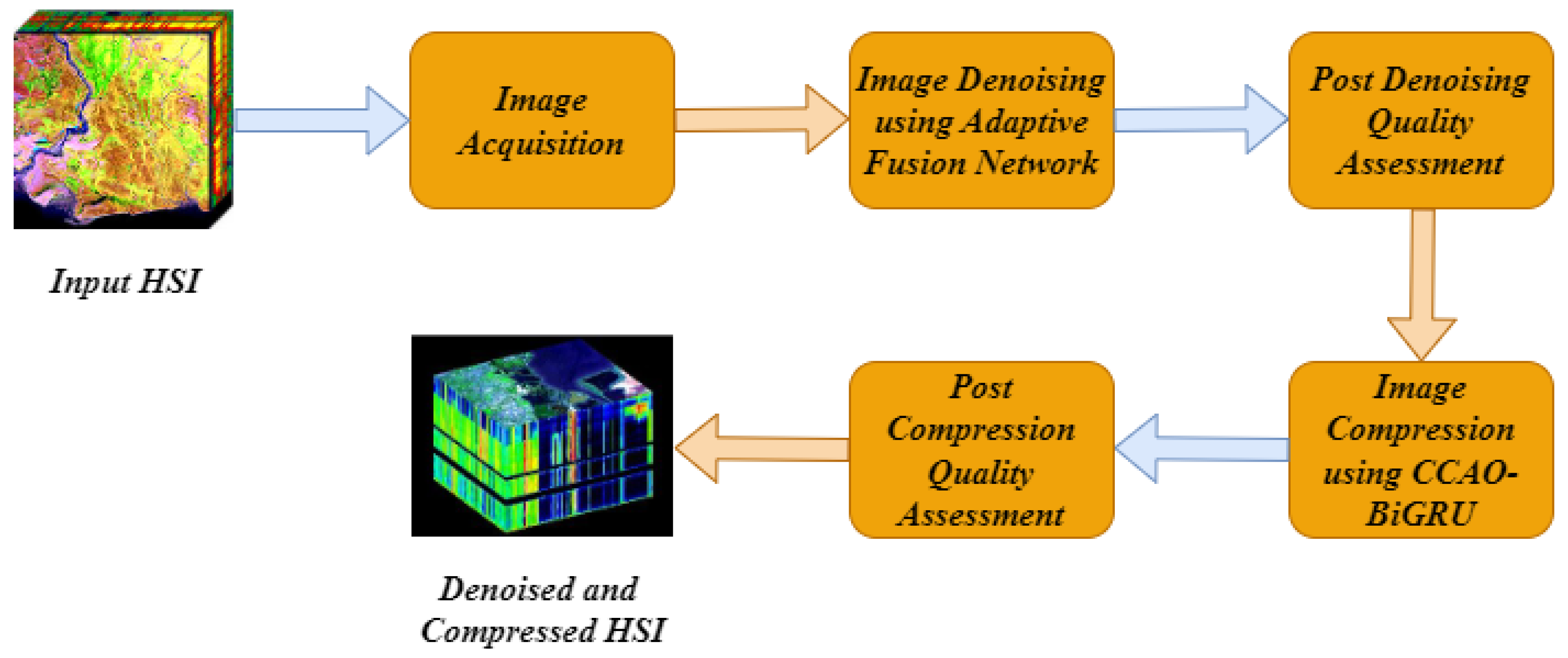
In the proposed method, the denoising and compression of HSI is modeled in the plan to create an effective model to obtain high-quality results compared to existing algorithms. The first stage after the acquisition is image denoising using improved adaptive fusion network. The denoised image is processed with compression in the next stage, and the chaotic Chebyshev artificial hummingbird optimization algorithm-based bidirectional gated recurrent unit is used to compress the HSI images. The proposed model is shown in the following Figure 1.

Figure 1.
Block diagram of proposed model.
2.2.1. Image Denoising
In the proposed model, different types of noise such as impulse noise, Gaussian noise, deadline noise, complex noise, stripes noise and mixed noise with a combination of Gaussian and impulse noise are applied to the input images. The improved adaptive fusion network [22] is used to remove noise from the HSI images. This network includes sublayers namely initial layer, coarse fusion network, fine fusion network and noise reconstruction. These four stages are combined together to identify the noisy images. By subtracting the noisy images from the observation data, noise-free data is generated.
Initial Layer and Coarse Fusion Network
The original HSI image is given to the initial layer of image denoising model as input. Initially, the images are downsampled into 1/2 and 1/4 scales with the help of Gaussian kernels. Here, multiple parallel convolutions are used to extract shallow features and deep features are then collected by the coarse fusion network. The fusion of the different scale information through several parallel adaptive instance (AIN) modules is performed by this layer. There are two main steps for designing a coarse fusion attention network. In the first step, the receptive field can be equipped by multiscale structures to capture more contents. In the second stage, the transfer of basic structure from low resolution feature maps to high resolution feature maps is carried out by the AIN module. This can be constructed by the AIN normalization technique, which is an efficient and compact model. The normalized feature maps can be performed by AIN normalization by taking input . Here, the width and height of the feature map are represented by X and K. The number of channels can be denoted by D. The downscale features should be identified. The current feature and downscale features are taken as inputs for AIN normalization. At first, the downscale features are converted into the size of by transposed convolution so as to have same dimensions of k. The parameters of affine transform from the transformed are calculated for each pixel (shift and scale ) by using contextual semantic information in downscale features. Each feature map is channel-wise normalized and pixel-wise affine transformed. At position (p,q,d), the updated values in the feature map are mathematically expressed as in Equation (1).
Here, the mean of k in channel d is denoted by , the standard deviation of the features in channel d is represented by . The can be mathematically calculated using Equation (2).
where is mathematically expressed as in Equation (3).
Here, the generated pixel-wise parameters from are noted as and which can handle spatially variant noise in images adaptively. The application of the convolutional layer is performed in , and for transferring feature information, the residual connection is used more effectively.
Fine Fusion Network
The coarse fusion network output is passed to the fine fusion network as input and multiple scale information refining is performed. The collection of multiscale information is passed into deep networks. Exchanging information across parallel multiresolution sub-networks is performed to conduct repeated multiscale fusion. The coattention fusion module is created to adaptively focus attention on informative features from multiple scales and improve the differential learning capability of network for image denoising. The fine fusion network initialized with multiscale features is represented as . Here, the spatial resolution index is denoted by s. The feature is represented as in the second layer. Each single feature representation is mathematically expressed in the following Equation (4).
Here, the coattention fusion module is denoted by DB and the transform function is denoted by . The identity connection can be obtained by input and output with the same resolution. The feature maps from multiple scales in the same size are passed into the coattention fusion module after transformation. The coattention fusion module contains two stages, namely concatenation and split, and fusion and self-calibration. In the first one, the trainable weights for feature fusion can be generated by receiving multiscale features in the coattention fusion module. The input features , and are with size of . The concatenation operation on three features can be mathematically expressed in the following Equation (5).
Here, the concatenation operation can be denoted by . The channel-wise details along spatial dimensions of are computed by global average pooling. The compact feature is generated by downsampling the convolutional layer. The feature v is passed into three parallel upsampling layers and provided with three feature descriptors, , and , with dimension . The three attention activation vectors , and are applied to the softmax function , and . In the fusion and self-calibration stage, three attention activation function vectors are developed. The input features are recalibrated using them as represented in the following Equation (6).
The architecture of the improved adaptive fusion network is shown in Figure 2.
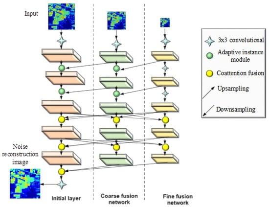
Figure 2.
Architecture of the improved adaptive fusion network.
The self-calibration module is used to correct and combine the features, which is represented in Equation (7).
Here, the self-calibrated convolution is denoted by . After fusion, the fused feature maps are operated with filters to improve the feature representation ability by self calibration convolution. This module transfers input features into firm descriptors and develops a set of three weights to construct channel-wise dependence.
Noise Reconstruction
The multiscale features are combined together by coattention module at the end of previous network. Then the residual noise images is learned. From the observation , the noise-free image is evaluated by subtracting . The optimization of network and reconstruction loss can be performed by loss which is mathematically expressed as in the Equation (8).
Here, the estimated noise-free HSI is denoted by and the real noise-free HSI is represented by P. The direction differences in spatial and spectral dimensions can give additional complementary support for denoising. The global gradient regularizer to describe the details of is expressed mathematically in Equation (9).
Here, gradient operators along horizontal, vertical, and spectral directions are denoted by , , and and the total loss function is mentioned in Equation (10).
Here, the weight parameter of is denoted by and is set to 0.01 to balance the loss terms.
2.2.2. Image Compression
The HSI image compression is performed using the chaotic Chebyshev artificial hummingbird optimization algorithm-based bidirectional gated recurrent unit (CCAO-BiGRU). The denoised image is directly given as input to the compression model.
Chaotic Chebyshev Artificial Hummingbird Optimization Algorithm-Based Bidirectional Gated Recurrent Unit
GRU is used to solve vanishing gradient problems in RNNs (recurrent neural networks). The reset gate and update gate are included in the GRU cell model. The activation gates depend on present and prior input. The hidden layers and input vectors in GRU cell are represented by and from the time slices m, implies the candidate of hidden state. The reset gate for m parts identifies the preceding data and the update gate updates the hidden state with current HSI images. These parameters are represented in Equations (11)–(14).
Here, the hyperbolic tangent and sigmoid function is denoted by and . The matrix multiplication and Hadamard product is represented by and *. The concatenation of two vectors and the weighted matrix learned by the GRU model are represented by , and , respectively.
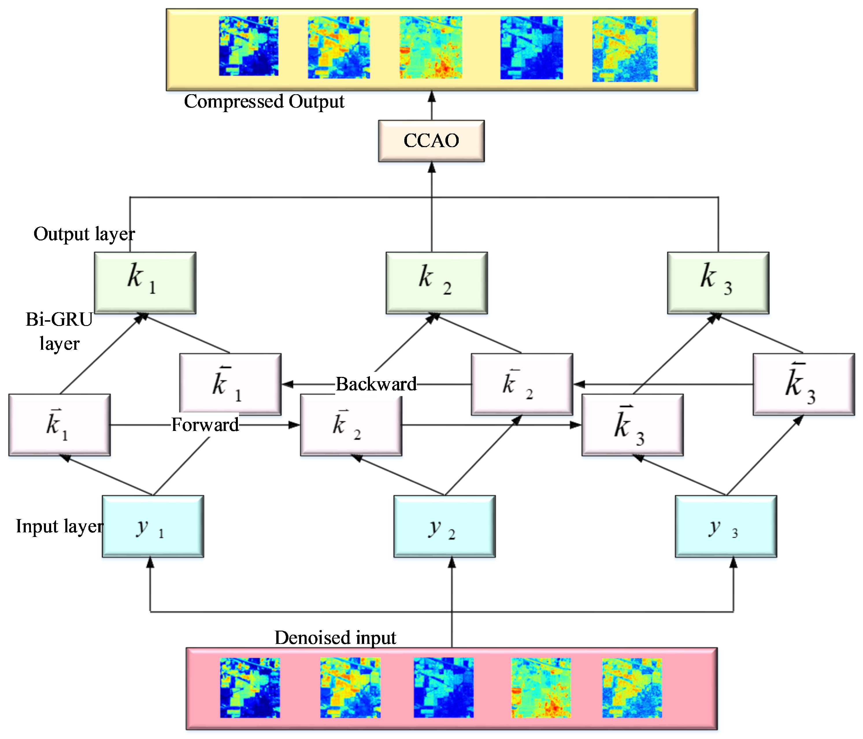
The GRU model [31] can read the data in only one direction. So, in order to increase data transmission, BiGRU layers have been added. The BiGRU model is used to improve the transfer of data in both forward and backward directions. The hidden layer contains two units with same input and connects with same output. The BiGRU forward and backward direction is denoted in Equation (15).
Here, the forward gated recurrent unit is denoted by and backward gated recurrent unit is denoted by . The image can be compressed by the BiGRU model and after image compression, it is passed in to artificial hummingbird optimization to receive the optimal output. The artificial hummingbird is a new metaheuristic algorithm that has the ability to fly and provide intelligent feeding methods of hummingbirds. There are three types of flight skills such as diagonal, axial and omnidirectional. These skills are employed in foraging strategies. Next, three different strategies are employed, such as territorial foraging, guided foraging, and migratory foraging. The architecture of the CCAO-BiGRU model is shown in Figure 3. The mathematical equation of the artificial hummingbird algorithm is described with the initial population of Z hummingbirds out of individuals as shown in Equation (16).
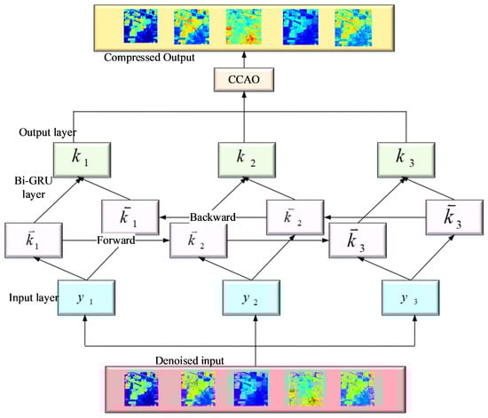
Figure 3.
Architecture of the CCAO-BiGRU model.
Here, the upper and lower bounds for C dimension are represented by E and V. The random vector in the range of [0, 1] is denoted by s. The visited table of food sources is represented in the following Equation (17).
Here, the value of becomes null for p = q, and becomes zero at . Here, p stands for hummingbird visiting food sources q.
In guided foraging, three flight directions such as diagonal, omnidirectional and axial flight are utilized. The BiGRU preserves the spatial dimension of the original image which helps to minimize the compression error. Also, the fine tuning of BiGRU using the proposed CCAO algorithm compresses the image more efficiently using the best global solution. This is accomplished through the balanced exploration and exploitation phase.
This CCAO-BiGRU model helps to compress the denoised images obtained from the improved adaptive fusion network phase. The image compression leads to provide a reduced size of the image without removing any quality of the images. After compressing the images, the quality of the image can be enhanced by the CCAO deep learning-based optimization algorithm. The exploration and exploitation phase in this algorithm is utilized to obtain better output. The loss function of the network model can be optimized through the integration of the hybrid chaotic Chebyshev artificial hummingbird optimization algorithm. A set of weights is applied to the network model to produce the high-quality compressed images. These weights sometimes create loss functions that lead to reduce the compressed image quality. This optimization algorithm is used to tune the hyperparameters in the model by reducing the loss function. Thus, by using the hybrid optimization model, optimal output can be produced with an enhanced quality of compressed images by updating the positions of the chaotic Chebyshev function in the artificial hummingbird algorithm. Thus, the compressed image quality can be further improved by integrating the optimization algorithm. The pseudocode for CCAO is represented in the following Table 2.
Table 2.
Pseudocode for CCAO algorithm.
2.3. Performance Analysis
Several performance metrics are analysed, which are described in the following section.
2.3.1. PSNR
PSNR is used to evaluate the quality between compressed images and original images. It is mathematically expressed in the following Equation (18).
where shows the number of spectral bands, shows the maximum pixel value of the th band, indicates the mean square error (MSE) between the processed and original image of the th band.
2.3.2. SSIM
It is used to calculate connection between two images and the mathematically represented as in the following Equation (19).
and are the mean or average values of the images p and q, and are the variances of p and q, and are the constants set to 0.0001 and 0.0009.
2.3.3. SAM
SAM compares test image spectra to a known reference spectra using spectral angle and this method is not sensitive to illumination. The mathematical expression is given below as in Equation (20).
indicates the dot product between the noisy and denoised spectra and , indicates the binary norm.
2.3.4. RAE
The performance of the predictive model is evaluated by the RAE parameter and is expressed using the following Equation (21).
indicates spectral band count, and show the HSI spatial resolution and and are the points at the ith spectral band with coordinates .
2.3.5. Compression Ratio (CR)
It is described as the ratio of the original image size to the compressed image size, as given in Equation (22).
3. Results
This section presents the results of the various stages of proposed method. Section 2.3 explains the metrics used for performance evaluation and the results are displayed as follows. The results of the proposed method have also been analysed by comparing with the existing methodologies and described in the following section.
3.1. Evaluation of Indian Pines Hyperspectral Dataset
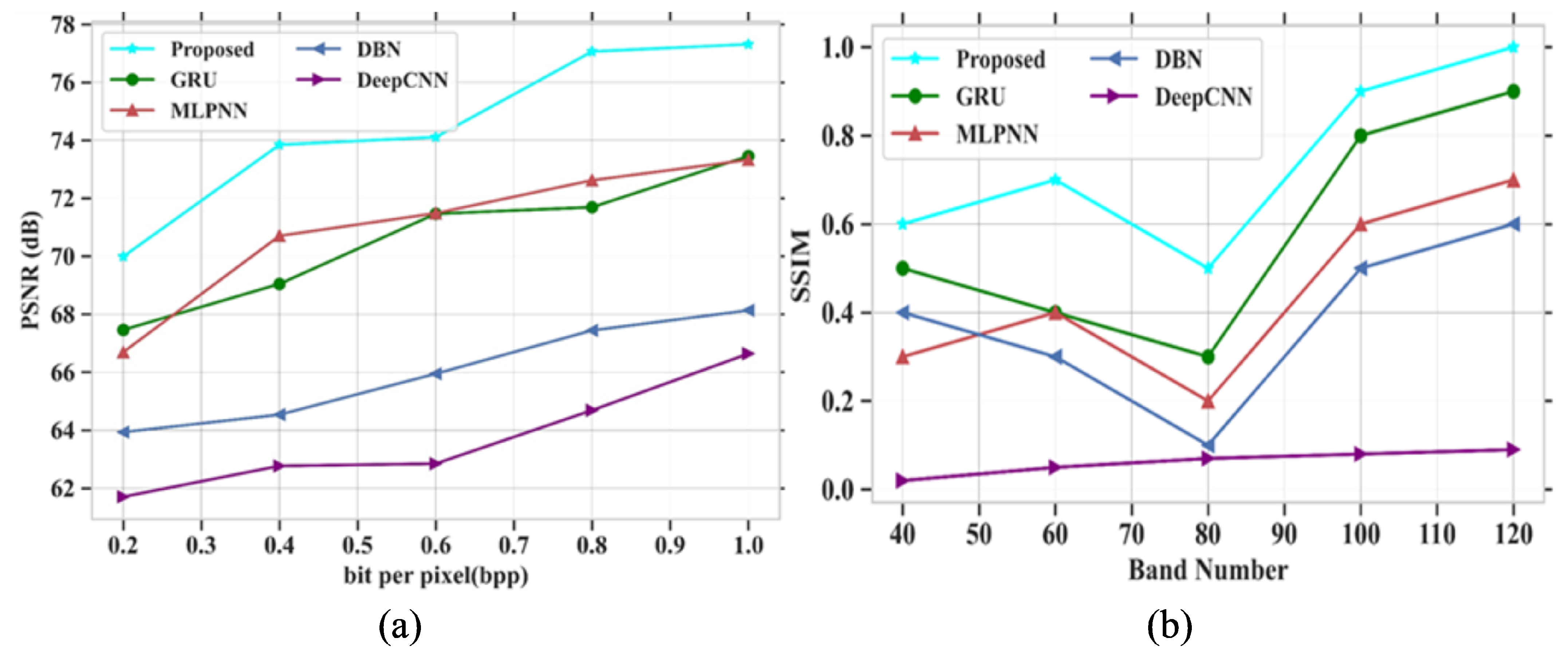
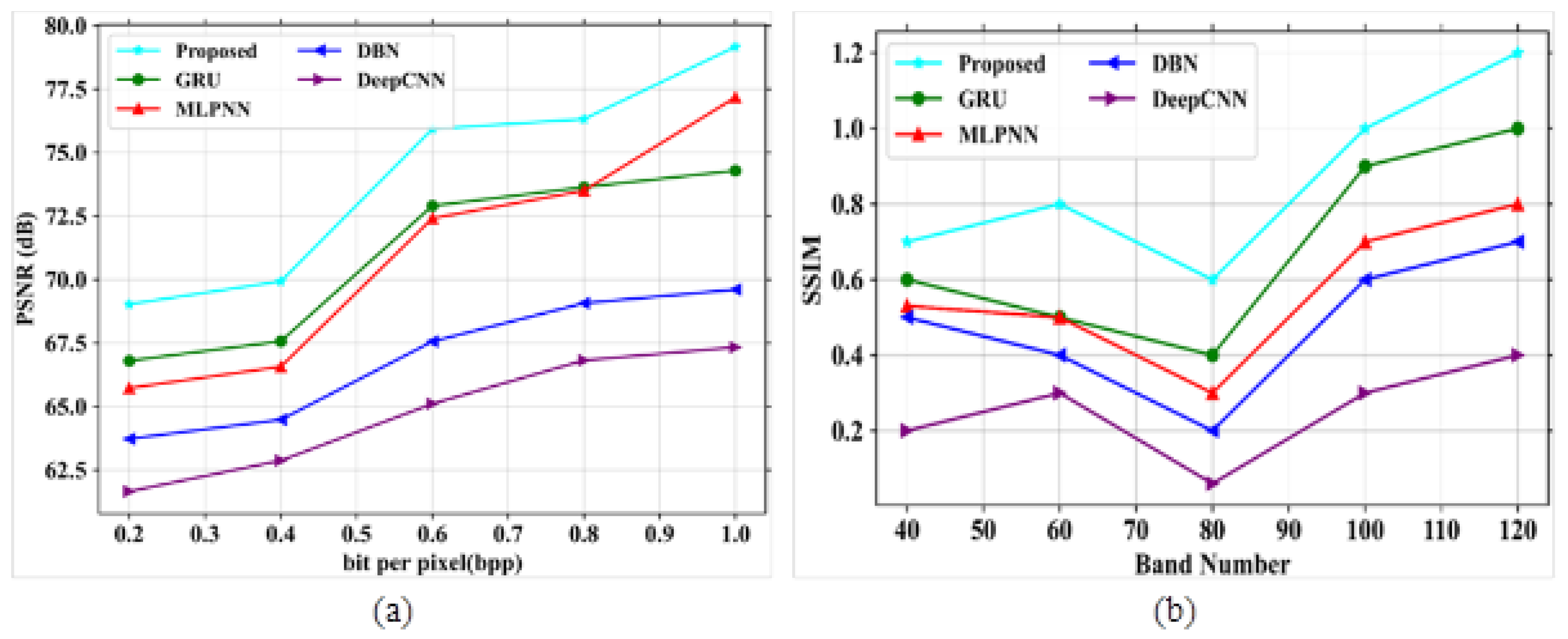
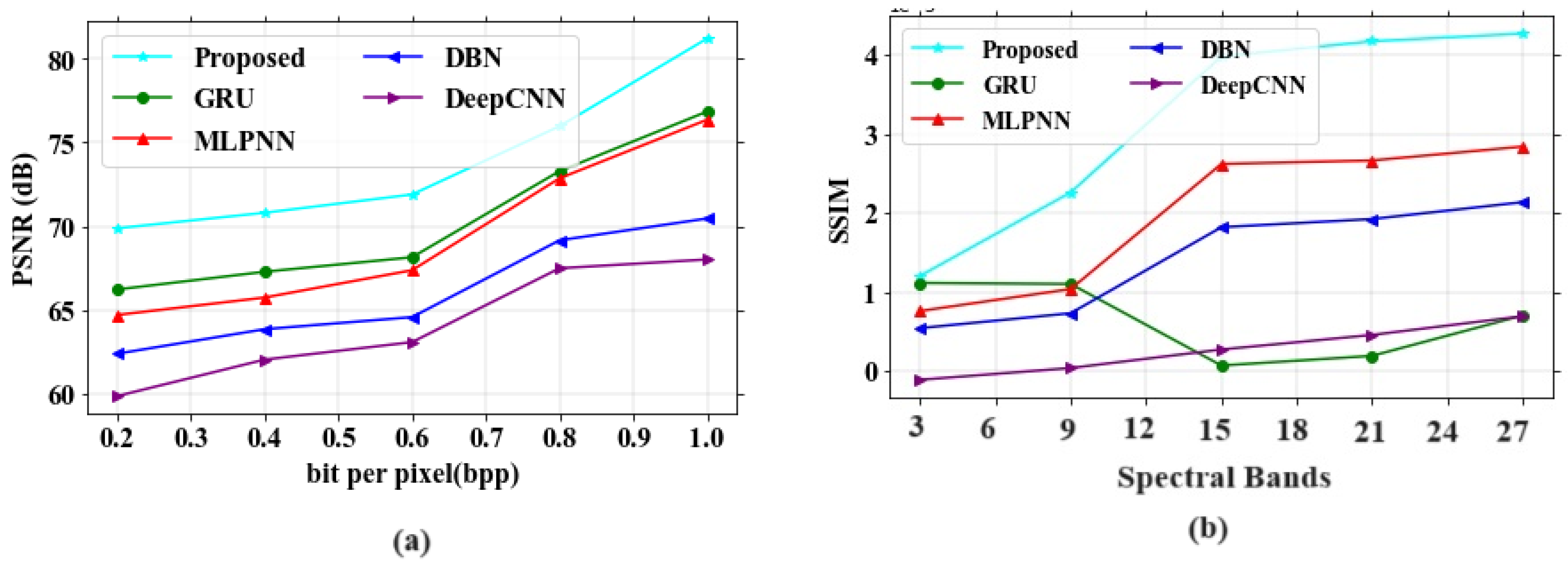
To analyze the proposed model, PSNR and SSIM are compared with different existing models like GRU, MLPNN, DBN and DeepCNN [32] using the Indian Pines hyperspectral dataset. Figure 4a,b depict the analysis of PSNR and SSIM parameters for existing and proposed models. The performance analysis with values for PSNR and SSIM is represented in Table 3.
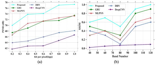
Figure 4.
Performance outcomes (a) PSNR vs. bit per pixel; (b) SSIM vs. band number.
Table 3.
PSNR and SSIM analysis.
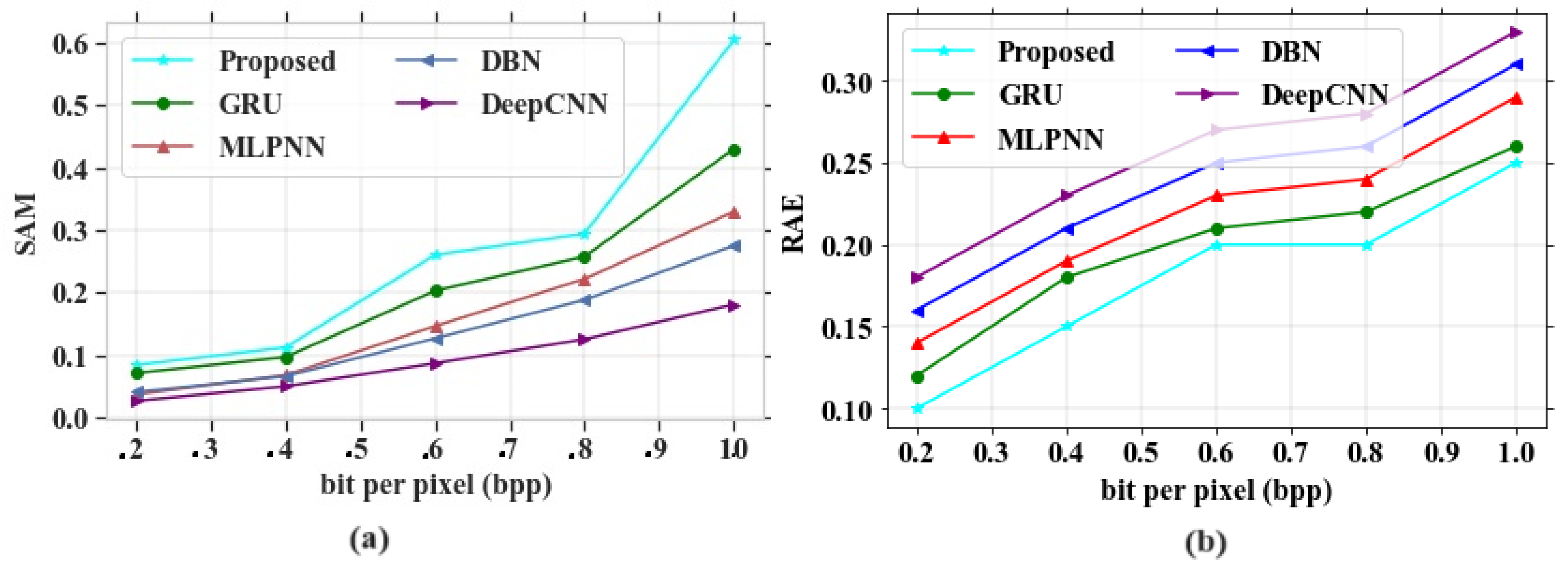
In Figure 4a, the existing models such as GRU, MLPNN, DBN and DeepCNN attained PSNR values of 73.45 dB, 73.32 dB, 68.13 dB and 66.63 dB at a bpp value of 1.0. If the bpp value is high, then the PSNR value also increases based on model performances. The proposed model obtained a PSNR value of 77.31 dB at a bpp value of 1. The proposed model gained higher PSNR values than other existing models. Figure 4b depicts the analysis of SSIM parameters against the band number. The existing models GRU, MLPNN, DBN and DeepCNN gained SSIM values of 0.9, 0.7, 0.6 and 0.09 at the number of band of 120, respectively. Finally, at the band number at 120, the proposed model obtained a SSIM value of 1.0. Figure 5 represents the analysis of SAM and RAE for different proposed and existing models. The comparison table for SAM and RAE is given in Table 4.
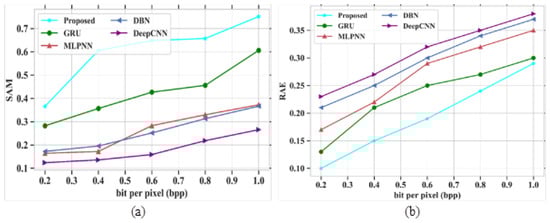
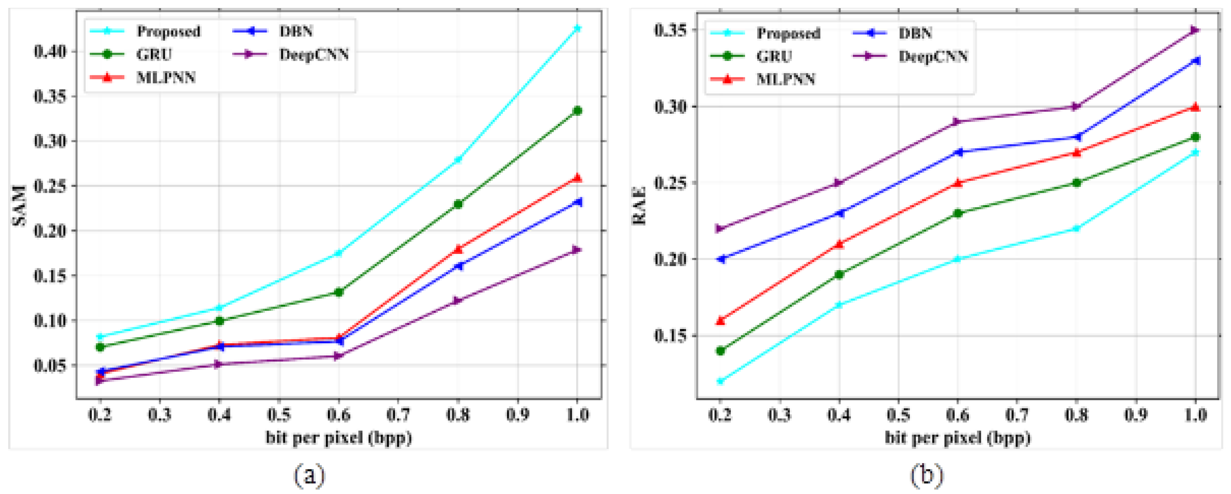
Figure 5.
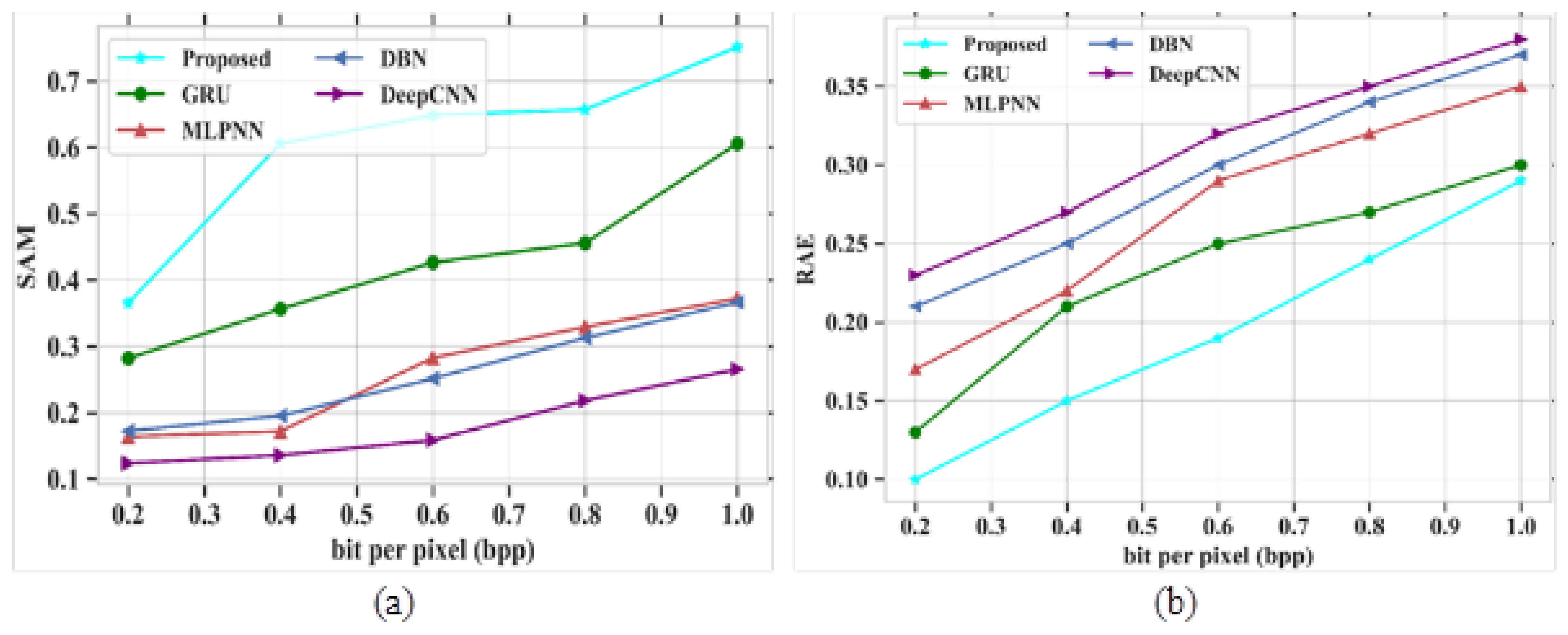
Performance evaluation (a) SAM vs. bit per pixels; (b) RAE vs. bit per pixels.
Table 4.
SAM and RAE analysis.
Figure 5a depicts the performance outcomes of the SAM parameter for the proposed model, which is compared with different existing models based on bpp range. Some of the existing models, like GRU, MLPNN, DBN and DeepCNN, obtained values of 0.6, 0.36, 0.32 and 0.6 at a bpp value of 1.0, respectively. The proposed model obtained a value of 0.75 at a bpp value of 1.0. In this analysis, the proposed model gives higher performances than other models. Figure 5b signifies the evaluation of the RAE parameter for proposed and existing models. The methods such as GRU, MLPNN, DBN and DeepCNN attained RAE values of 0.3, 0.35, 0.37 and 0.38 at a bpp of 1.0. The proposed model shows fewer errors and it gives a RAE value of 0.29 at a bpp value of 1.0. As the proposed model gives better results than the other existing models, it is proved to be an efficient technique for HSI compression.
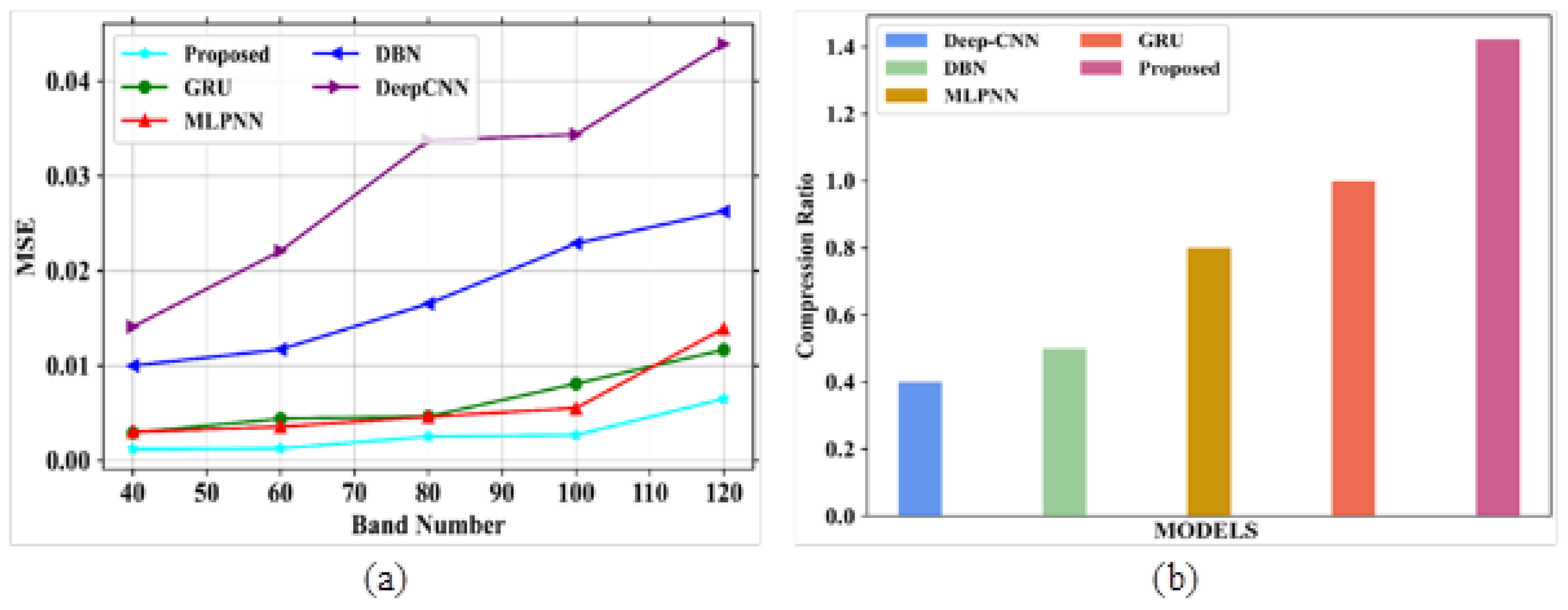
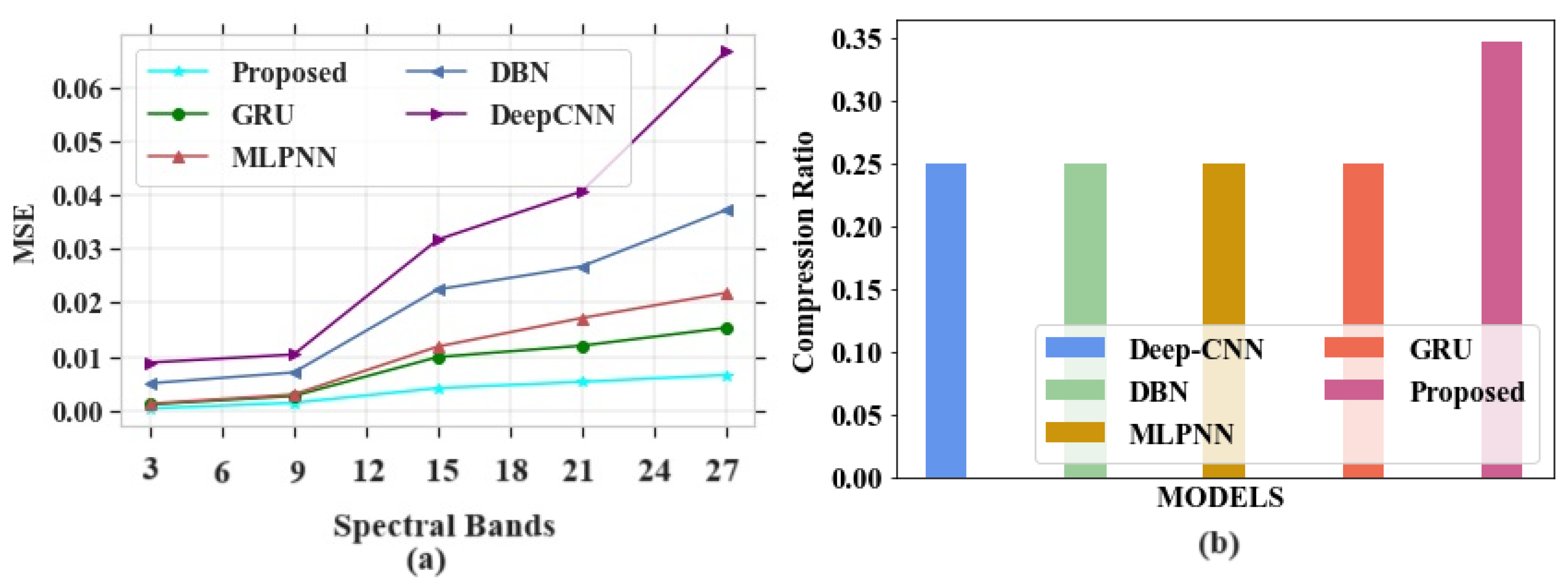
Figure 6a,b signifies the analysis of MSE and CR for different existing and proposed models. Table 5 depicts the comparison of MSE and CR.
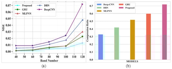
Figure 6.
Performance outcomes (a) MSE vs. spectral bands; (b) compression ratio (CR).
Table 5.
MSE vs. band number and compression ratio comparison.
Figure 6a depicts the performance evaluation of MSE for proposed and existing models. The existing models like GRU, MLPNN, DBN and DeepCNN attained MSE values of 0.022, 0.03, 047 and 0.071 at a band number 120, respectively. The proposed model shows an MSE value of 0.013 at the same band number. From this comparison analysis, the proposed model succeeded in giving a lower error rate compared to existing models. Figure 6b signifies the analysis of CR for proposed and existing models. The existing models, such as GRU, MLPNN, DBN and DeepCNN, gained CR levels of 0.6, 0.52, 0.42 and 0.33, respectively.The proposed model attained a CR of 0.72. In this analysis, the proposed model gives higher CR values than other models without compromising the quality of the images.
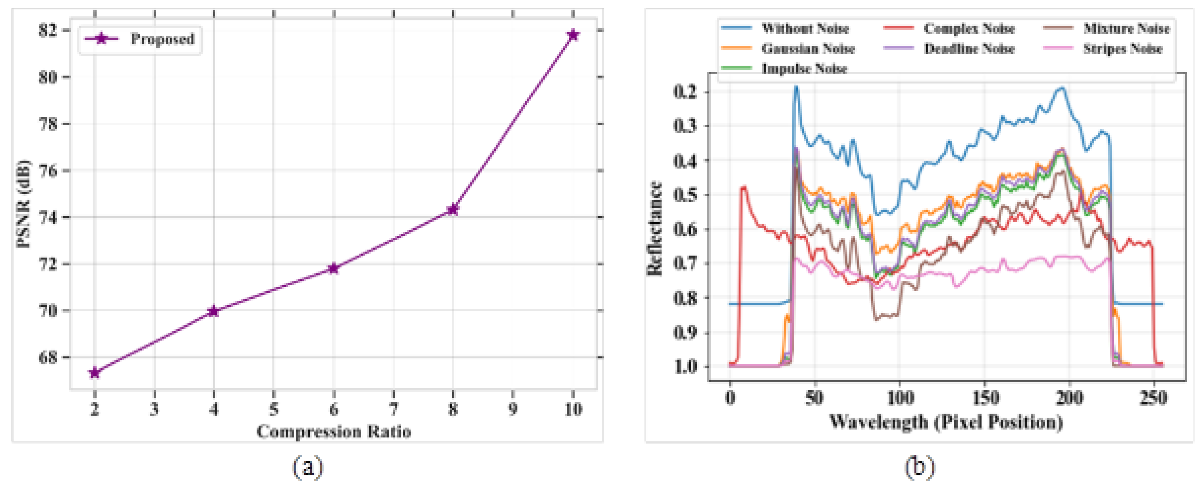
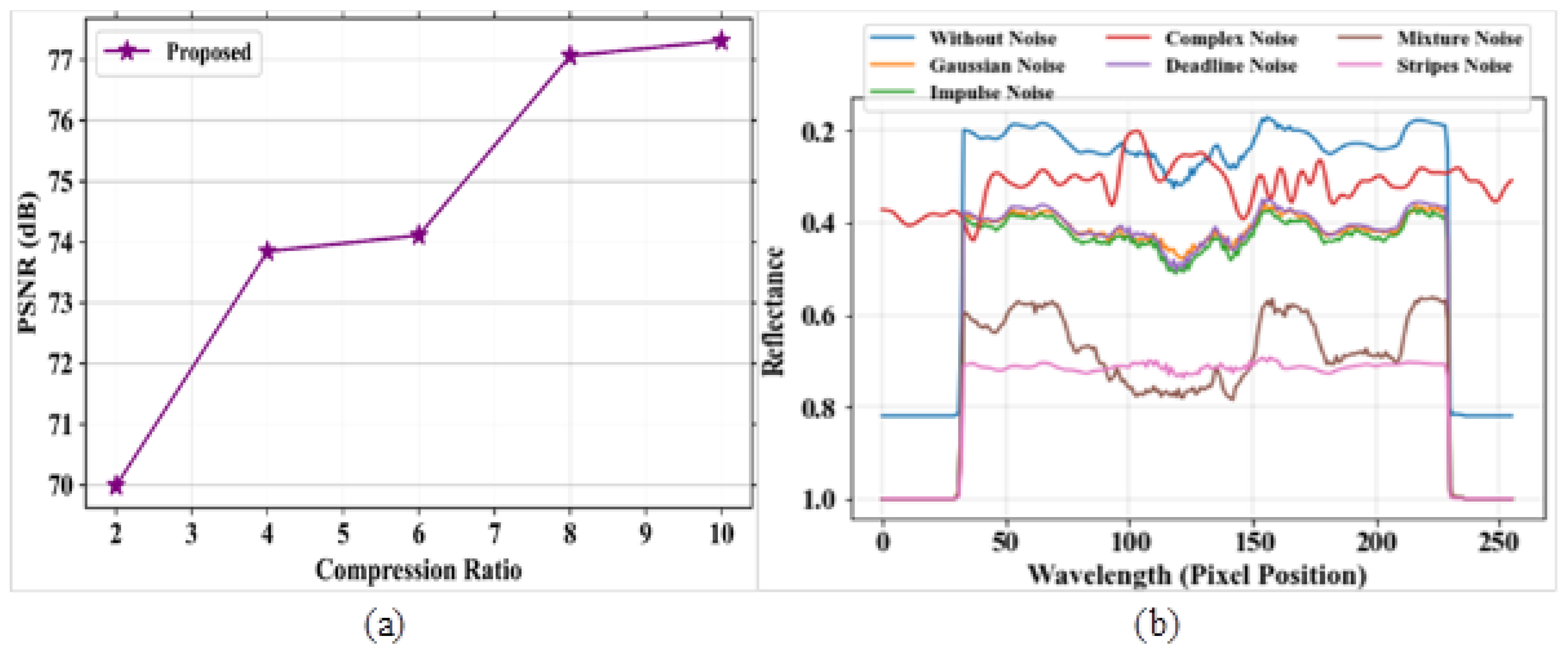
Figure 7a,b signifies the outcome of PSNR for the proposed model and reflectance graphs for different types of noise. The comparison table for PSNR analysis based on the compression ratio is represented in Table 6. Figure 7a represents the analysis of the PSNR parameter for the proposed model based on compression ratio. The PSNR value is evaluated for a compressed image to measure the image quality. The PSNR increases with the increase in compression ratio. The proposed model obtained a high PSNR value of 82 dB at a compression ratio of 10. Figure 7b depicts the analysis of the reflectance value versus different noises, such as complex noise, Gaussian noise, mixture noise, deadline noise, stripes noise, and impulse noise. The reflectance value is high at the lower wavelength level.
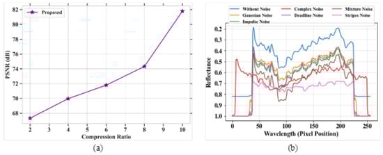
Figure 7.
Performance outcomes (a) PSNR vs. compression ratio; (b) reflectance vs. pixel position.
Table 6.
Performance evaluation of PSNR with CR.
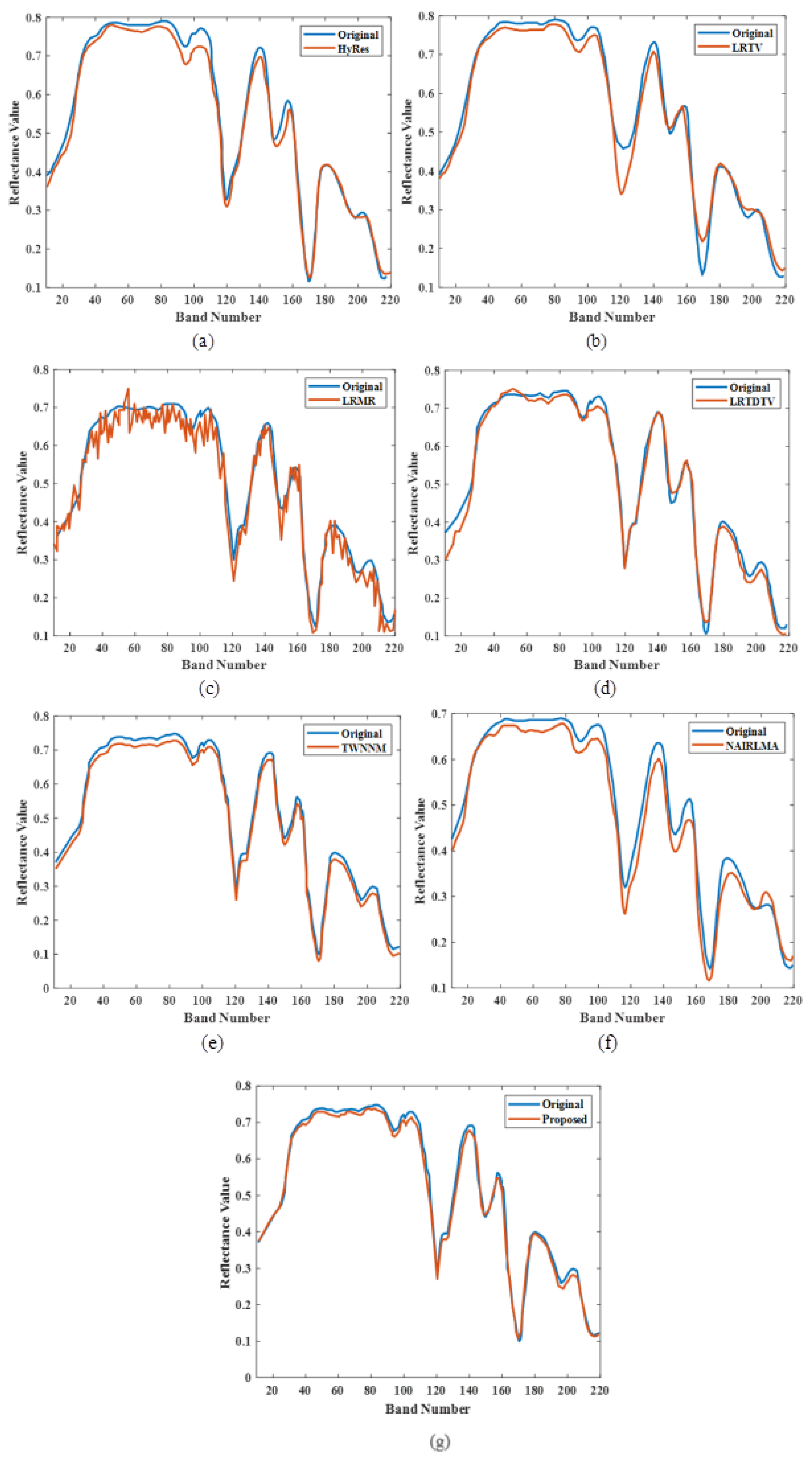
Figure 8a–g [16] shows the analysis of the spectral reflectance curve for the proposed model and existing models, based on the number of bands. Figure 8a–g, represents the analysis of spectral reflection. Here, the original spectral reflectance curve is denoted in blue, and the orange curve represents the denoised spectral reflectance. The spectral reflectance is analysed for several existing models, such as TV-regularized low-rank matrix factorization (LRTV), low-rank matrix recovery (LRMR), automatic hyperspectral image restoration (HyRes), noise-adjusted iterative low-rank matrix approximation (NAILRMA), tensor-weighted nuclear norm minimization (TWNNM), and total variation regularized low-rank tensor decomposition (LRTDTV), as well as for the proposed study. Thus, the proposed model shows the best results compared to all other methods.
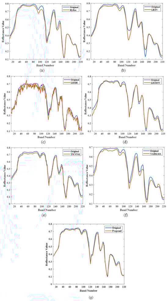
Figure 8.
Performance outcomes of spectral reflection.
3.2. Evaluation of Washington DC Mall Dataset
The performance analysis for different parameters have been performed and are described in the following section. Figure 9a,b signifies the analysis of PSNR and SSIM. The performance comparison is represented in Table 7.
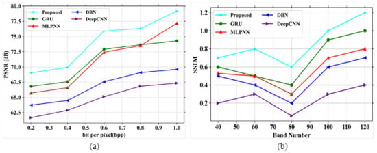
Figure 9.
Performance outcomes (a) PSNR vs. bpp; (b) SSIM vs. band number.
Table 7.
Showing PSNR vs. bpp and SSIM vs. band number.
In Figure 9a, the existing models like GRU, MLPNN, DBN, and DeepCNN obtained values of 74.29 dB, 77.17, 69.6 dB and 67.33 dB at 1.0 bpp, respectively. The proposed model gained a value of 79.16 dB at 1.0 bpp. In Figure 9b, the existing models obtained SSIM values of 1, 0.8, 0.7 and 0.4 for a band number 120, respectively. The proposed model showed a SSIM value of 1.2 for the same band number. Figure 10a,b depict the analysis of SAM and RAE for the proposed and existing models, as shown in Table 8.
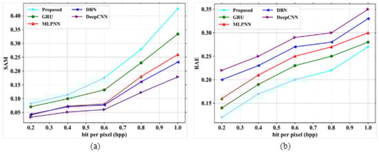
Figure 10.
Performance outcomes (a) SAM vs. bpp; (b) RAE vs. bpp.
Table 8.
Comparison table for SAM vs. bpp and RAE vs. bpp.
In Figure 10a, the existing models such as GRU, MLPNN, DBN and DeepCNN obtained SAM values of 0.317, 0.282, 0.256 and 0.202 based on bpp range at 1.0, respectively. The suggested model can attain the highest value of 0.35 at bpp 1.0. In Figure 10b, the existing models gained RAE values of 0.28, 0.3, 0.33 and 0.35 at a bpp of 1.0, respectively. The proposed model showed a very low RAE value of 0.27 at the same bpp. Figure 11a,b depict the performance outcomes of MSE and compression ratio.
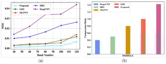
Figure 11.
Performance evaluation (a) MSE vs. band number; (b) compression ratio.
The comparison table for MSE vs. band number and compression ratio is represented in Table 9.
Table 9.
MSE vs. band number and compression ratio.
In Figure 11a, the existing models obtained the following values: GRU obtained 0.011, MLPNN attained a value of 0.0139, DBN obtained an MSE value of 0.026, and DeepCNN attained a value of 0.043, all at band number 120. The proposed model could attain an MSE value of 0.0065 at the same band number. In Figure 11b, GRU, MLPNN, DBN and DeepCNN attained CR values of 0.8, 0.5, 0.4 and 0.3, respectively whereas the proposed model obtained a CR of 1. Figure 12a,b depict the analysis of PSNR based on compression ratio and reflectance curve for different noises. The comparison table for PSNR analysis based on compression ratio is represented in Table 10.
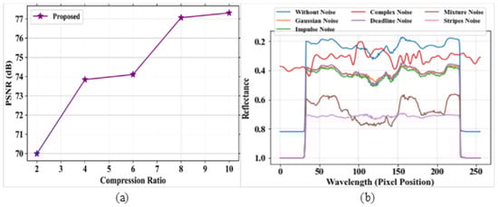
Figure 12.
Performance outcomes (a) PSNR vs. compression ratio; (b) reflectance vs. pixel position.
Table 10.
Performance evaluation of PSNR vs. CR.
3.3. Evaluation of CAVE Dataset
The performance analysis for different parameters have been performed and are described in the following section. Figure 13a,b signifies the analysis of PSNR and SSIM. The performance comparison is represented in Table 11.
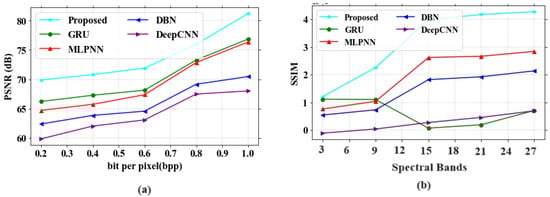
Figure 13.
Performance outcomes (a) PSNR vs. bpp; (b) SSIM vs. band number.
Table 11.
Showing PSNR vs. bpp and SSIM vs. band number.
In Figure 13a, the existing models like GRU, MLPNN, DBN and DeepCNN obtained values of 76.29 dB, 75.17, 71.39 dB and 69.33 dB at 1.0 bpp, respectively. The proposed model gained a value of 81.16 dB at 1.0 bpp. In Figure 13b, the existing models obtained SSIM values of 0.8, 2.9, 2.1 and 0.7, respectively, for a band number 27. The proposed model showed a SSIM value of 4.2 for the same band number.
Figure 14a,b depict the analysis of SAM and RAE for proposed and existing models as shown in in Table 12.
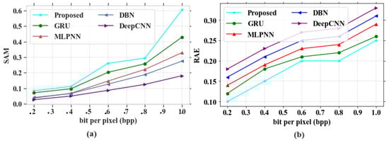
Figure 14.
Performance outcomes (a) SAM vs. bpp; (b) RAE vs. bpp.
Table 12.
Comparison table for SAM vs. bpp and RAE vs. bpp.
In Figure 14a, the existing models such as GRU, MLPNN, DBN and DeepCNN obtained SAM values of 0.42, 0.32, 0.28 and 0.18 based on a bpp range at 1.0, respectively. The suggested model can attain the highest value of 0.59 at bpp 1.0. In Figure 14b, the existing models gained RAE values of 0.26, 0.29, 0.31 and 0.33 at a bpp of 1.0, respectively. The proposed model showed a very low RAE value of 0.25 at the same bpp.
Figure 15a,b depict the performance outcomes of MSE and compression ratio. The comparison table for MSE vs. spectral bands and compression ratio is represented in Table 13.
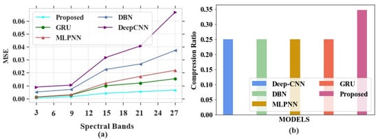
Figure 15.
Performance evaluation (a) MSE vs. spectral bands; (b) compression ratio.
Table 13.
MSE vs. spectral bands and compression ratio.
In Figure 15a, the existing models obtained the following MSE values: GRU obtained an MSE of 0.023, MLPNN attained a value of 0.021, DBN obtained an MSE value of 0.039, and DeepCNN attained a value of 0.063 at a band number of 27. The proposed model could attain an MSE value of 0.0085 at the same band number. In Figure 15b GRU, MLPNN, DBN and DeepCNN attained CR values of 0.27, 0.24, 0.26 and 0.25, respectively, whereas the proposed model obtained a CR of 0.35.
3.4. Ablation Experiments
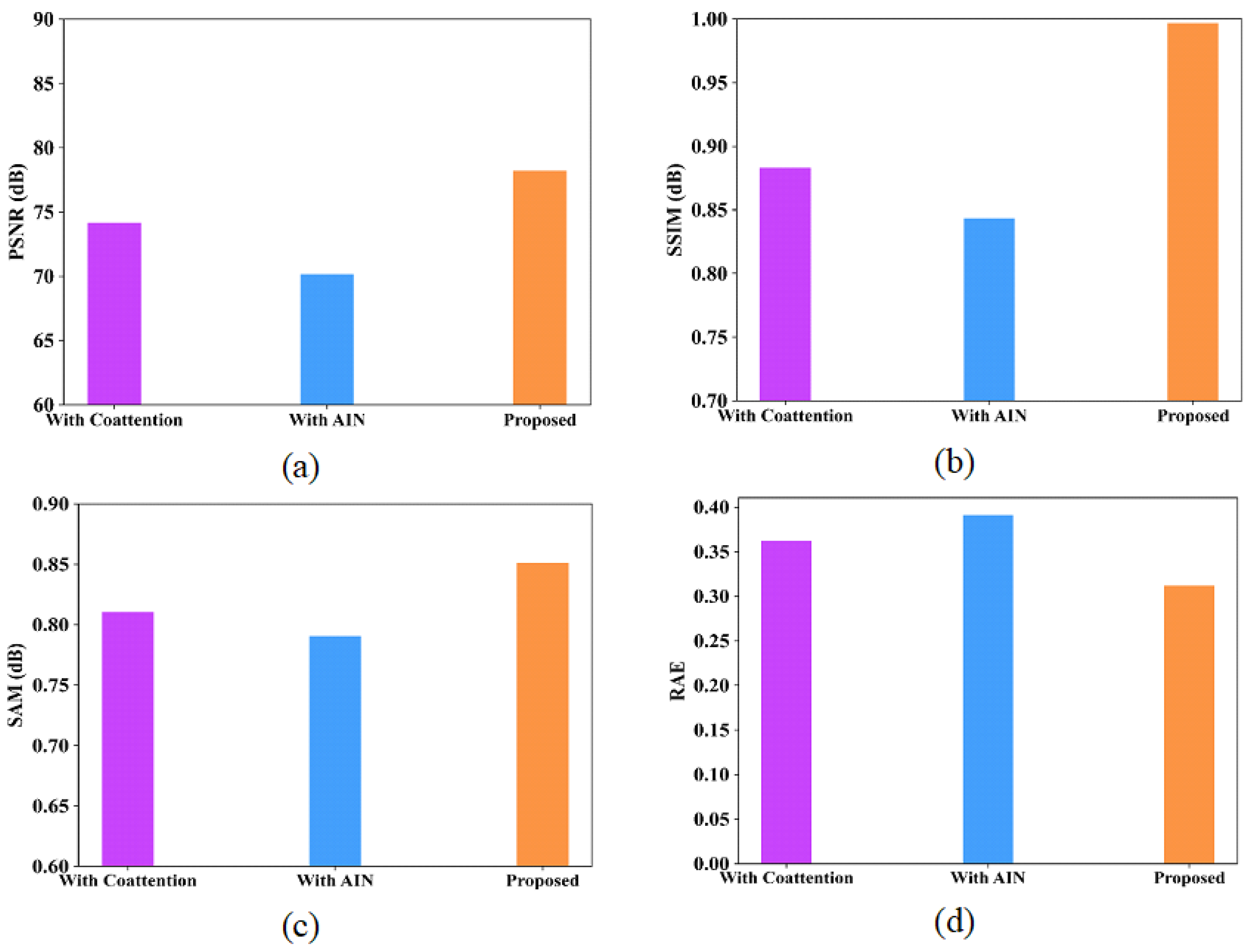
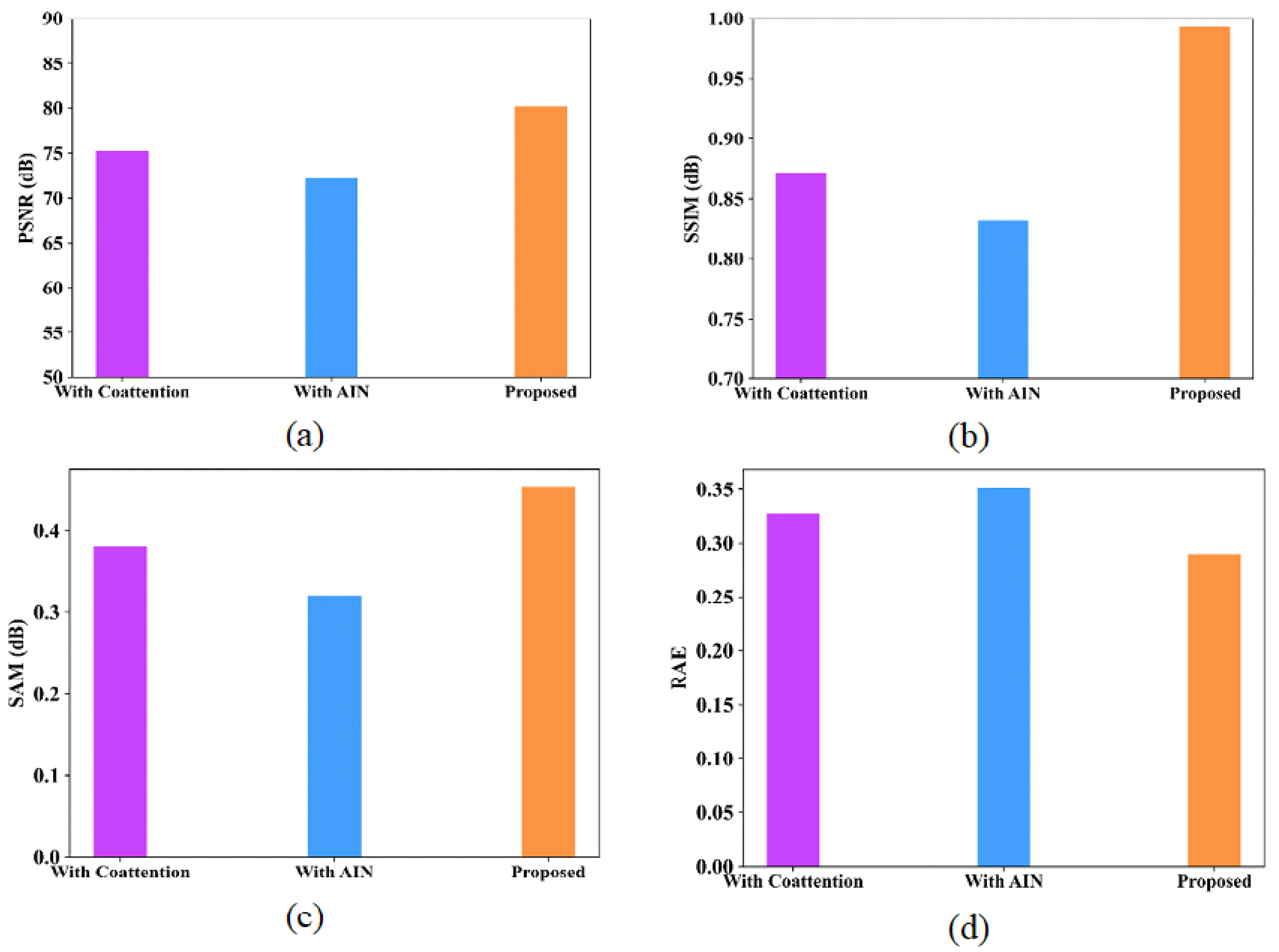
Ablation experiments are analyzed for the proposed model to provide deeper analysis in terms of various metrics like PSNR, SSIM, SAM and RAE. Table 14 and Table 15 represent the ablation study of the proposed model using the Indian Pines and Washington DC Mall datasets. Figure 16 and Figure 17 show the performance analysis of proposed model with coattention and AIN modules for the Indian Pines dataset and Washington DC Mall dataset, respectively.
Table 14.
Ablation study for the Indian Pines dataset.
Table 15.
Ablation study for Washington DC Mall dataset.
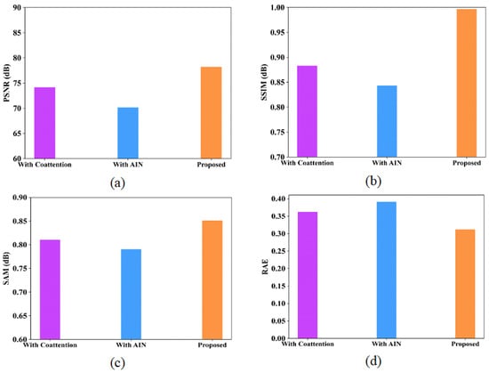
Figure 16.
Performance analysis of proposed model with coattention and with AIN (a) PSNR; (b) SSIM; (c) SAM; (d) RAE for Indian Pines dataset.
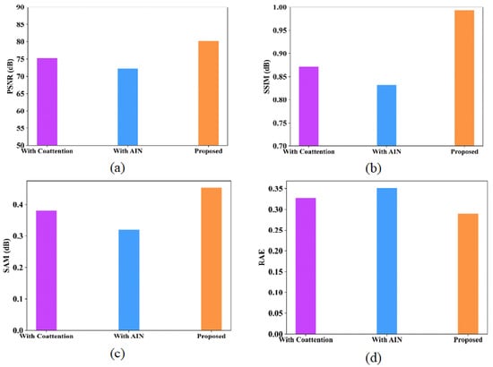
Figure 17.
Performance analysis of proposed model with coattention and with AIN (a) PSNR; (b) SSIM; (c) SAM; (d) RAE for Washington DC Mall dataset.
3.5. Computational Complexity
The computational complexity of the proposed model and existing models for the Indian Pines dataset and Washington DC Mall dataset is analysed in Table 16. The results are graphically represented for the Indian Pines dataset in Figure 18a and for the Washington DC Mall dataset in Figure 18b. The processing time is considerably lower for the proposed model.
Table 16.
Showing the comparison of computational complexity of proposed model with existing models for the Indian Pines and Washington DC Mall datasets.
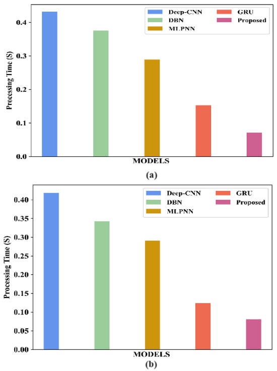
Figure 18.
Comparison of computational complexity of proposed model with existing models for (a) the Indian Pines dataset; (b) the Washington DC Mall dataset.
3.6. Visual Analysis
In this analysis, some of the sample input images are taken and their application on the proposed model is analysed qualitatively.
3.6.1. Sample Outcomes for Proposed Models Using Indian Pines Hyperspectral Dataset
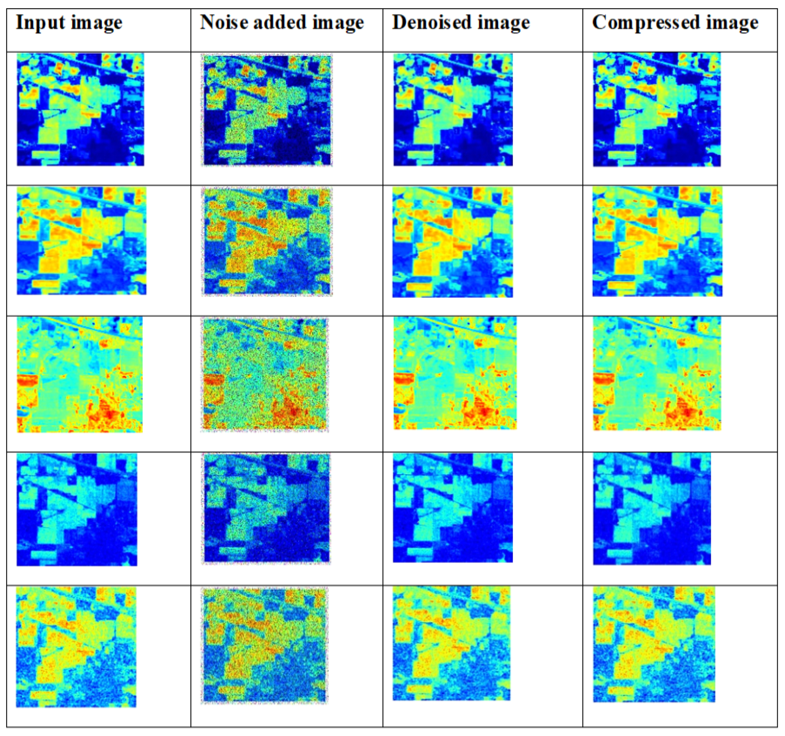
Some of the sample denoised and compressed output images for the Indian Pines hyperspectral dataset are shown in in Figure 19.
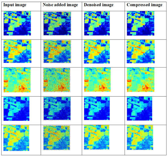
Figure 19.
Samples of input images, denoised images and compressed images for the Indian Pines HSI dataset.
The sample input images are collected from the Indian Pines hyperspectral dataset, which are denoised and compressed by the proposed model. The image denoising was performed by the improved adaptive fusion network, and image compression was performed by CCAO-BiGRU.
3.6.2. Sample Compression Outcomes for Different Noises Using Indian Pines Hyperspectral Dataset
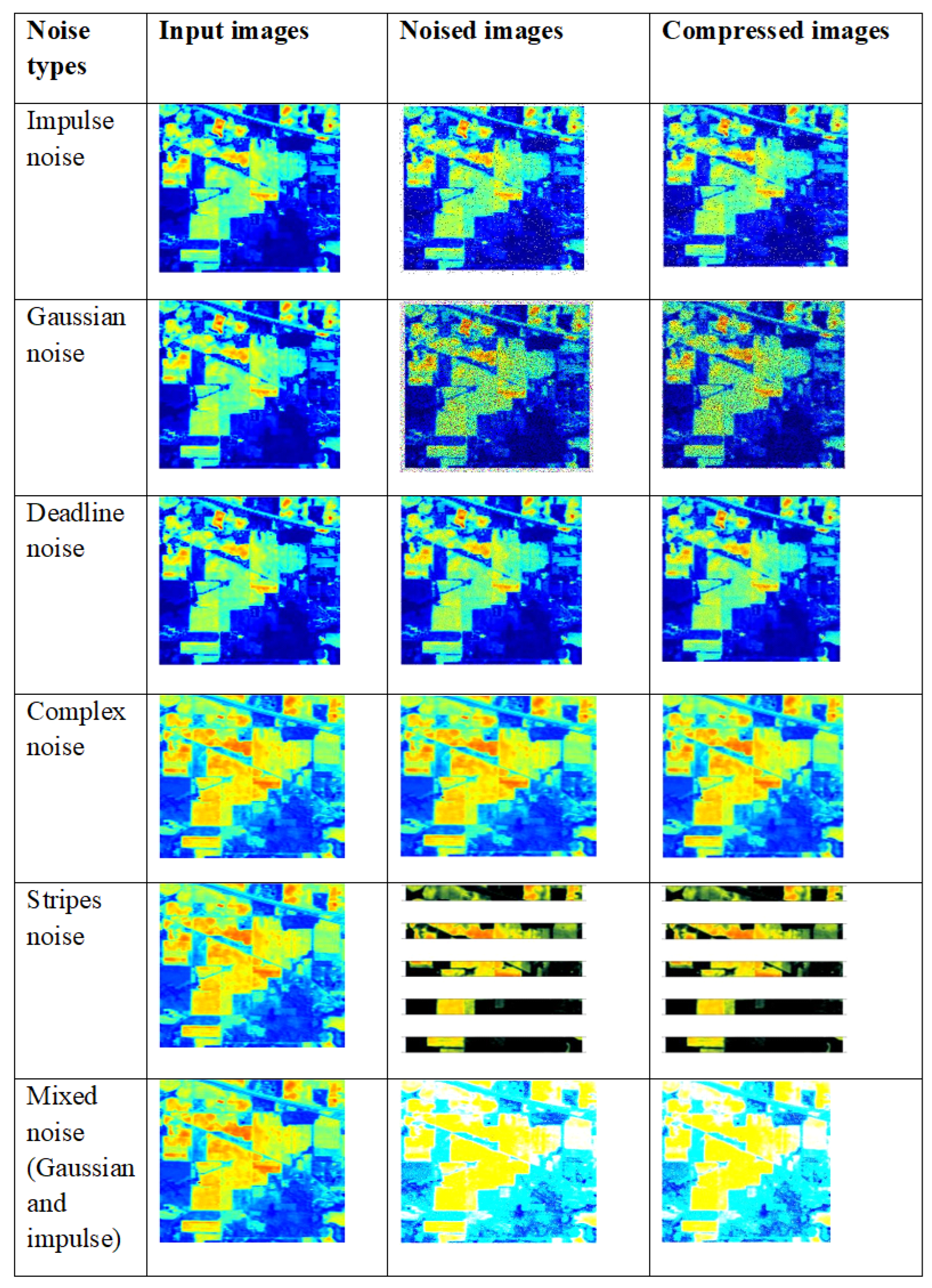
Various types of noises are applied to the input images, such as impulse noise, Gaussian noise, deadline noise, complex noise, stripes noise and mixed noise. The resultant denoised and compressed images are shown in Figure 20.

Figure 20.
Compressed output with various types of noise applied to input images using the Indian Pines hyperspectral dataset.
3.6.3. Sample Outcomes for Proposed Models Using Washington DC Mall Dataset
Some of the sample denoised and compressed output images for Indian Pines Washington DC Mall hyperspectral dataset are shown in in Figure 21.
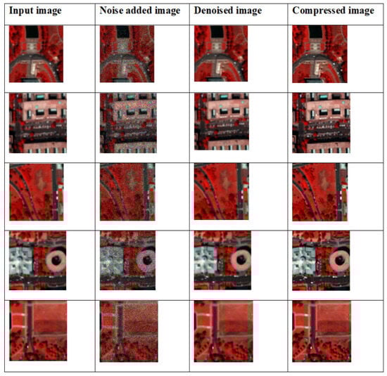
Figure 21.
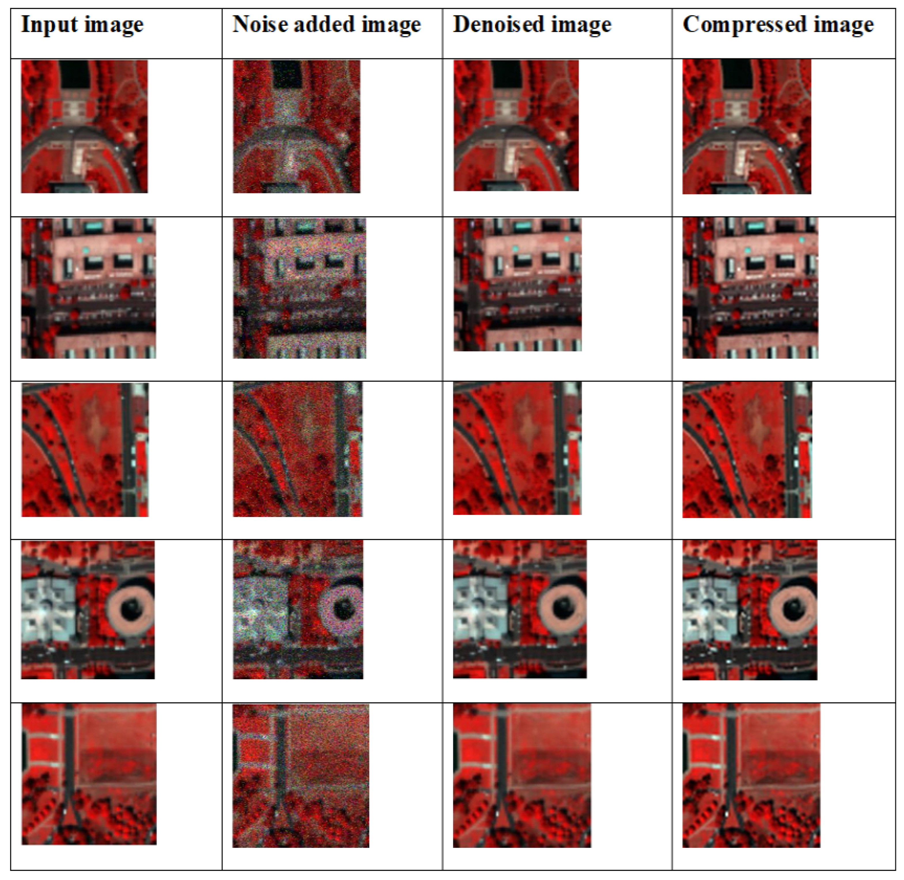
Samples of input images, denoised images and compressed images for the Washington DC Mall HSI dataset.
The sample input images are collected from the Washington DC Mall hyperspectral dataset, which are denoised and compressed by the proposed model. The image denoising was performed by the improved adaptive fusion network, and image compression was performed by CCAO-BiGRU.
3.6.4. Sample Compression Outcomes for Different Noises Using Washington DC Mall Hyperspectral Dataset
Various types of noises [33] are applied to the input images, such as impulse noise, Gaussian noise, deadline noise, complex noise, stripes noise and mixed noise. The resultant denoised and compressed images are shown in Figure 22.
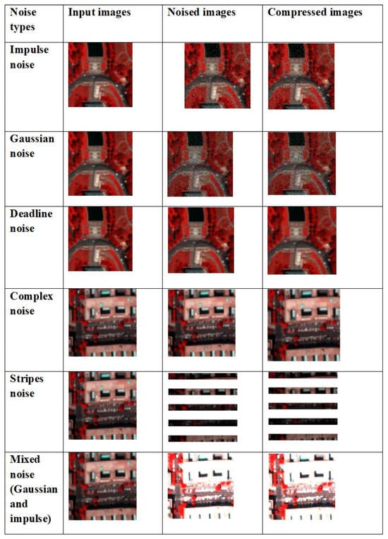
Figure 22.
Compressed output with various types of noise applied to input images using the Washington DC Mall hyperspectral dataset.
4. Discussion
The major aim of this research work is to denoise and compress the HSI images [34,35] with less processing time and without compromising the image quality. Here, several performance metrics are analysed for proposed and existing models. Taking the results of quantitative and qualitative analyses [36] into consideration, it can be shown that the proposed study provides better results. The two datasets, namely the Indian Pines dataset and Washington DC Mall dataset, were considered for the study. In the first stage, the input images were passed through an improved adaptive fusion network for noise removal. After denoising, the images were compressed with the CCAO-BiGRU model without reducing the quality of images [37,38]. Several drawbacks were noticed in the existing techniques, such as poor accuracy in image compression, improper compression of large size images, and the loss of important characteristics of images after compression. The proposed model obtained a PSNR value of 77.31 dB, a SAM of 0.7, a RAE of 0.29 at bpp 1.0, a SSIM of 1, an MSE at 0.013 at band number 120, a CR of 0.72, and the PSNR value based on a compression ratio at 10 is 82 for the Indian Pines dataset. For the Washington DC Mall dataset, the following values were obtained: PSNR of 79.16 dB, SAM of 0.35, RAE of 0.27 at bpp 1.0, SSIM of 1.2, MSE of 0.0065 at band number 120, CR of 1, and the PSNR value based on a compression ratio of 10 is 78.4. The proposed model obtained better values of PSNR, SAM, SSIR and RAE for both the datasets. It also gave a good plot of PSNR vs. CR curve which gives the impression of it being a better compression model. In addition, visual analysis also provided good results, which in turn proves the quality of the developed model. The proposed algorithm is compared with different existing methods in terms of quantitative metrics and it showed that the proposed model performs better compared to the existing models. The performance accuracy of the proposed work indicates that this can be utilized for mineral mapping as well as for agricultural applications. The PSNR values in [39] can be further improved using a different activation function.
5. Conclusions
In this study, a novel image denoising and compression technique based on a deep learning model is proposed to retain the overall quality of an image without limiting the compression ratio. Here, three datasets, namely the Indian Pines dataset, the Washington DC Mall dataset, and the CAVE dataset were considered for the study. In the first stage, an improved adaptive fusion network is used to remove undesirable noise from the images. In the second stage, the denoised image is passed into the compression phase. In the compression stage, the images are compressed without compromising the quality using the CCAO-BiGRU model. The performance metrics, such as PSNR, SSIM, MSE, CR, RAE and spectral reflectance curve for various types of noise were analysed for the proposed and existing models. From these analyses, we proved that the proposed model is a better system compared to the existing models. In future research, the replacement of the activation function in the proposed model (ReLU and sigmoid) with generalized divisive normalization (GDN) can be performed to improve the PSNR value further. Additionally, the proposed algorithm can be tested using real-time data.
Author Contributions
Conceptualization, A.J.; methodology, A.J.; software, D.M.; validation, A.J.; formal analysis, D.M. and S.R.; resources, D.M.; writing—original draft, D.M.; writing—review and editing, A.J.; supervision, A.J. and S.R.; project administration, S.R. All authors have read and agreed to the published version of the manuscript.
Funding
This research received no external funding.
Data Availability Statement
Data are contained within the article.
Conflicts of Interest
The authors declare no conflicts of interest.
References
- Vargas, H.; Ramírez, J.; Pinilla, S.; Torre, J.I.M. Multi-Sensor Image Feature Fusion via Subspace-Based Approach Using ℓ1-Gradient Regularization. IEEE J. Sel. Top. Signal Process. 2023, 17, 525–537. [Google Scholar] [CrossRef]
- Wang, W.; den Brinker, A.C. Modified RGB Cameras for Infrared Remote-PPG. IEEE Trans. Biomed. Eng. 2020, 67, 2893–2904. [Google Scholar] [CrossRef]
- Schmitt, B.; Souidi, Z.; Duquesnoy, F.; Donzé, F.V. From RGB camera to hyperspectral imaging: A breakthrough in Neolithic rock painting analysis. Herit. Sci. 2023, 11, 91. [Google Scholar] [CrossRef]
- Zhao, D.; Liu, S.; Yang, X.; Ma, Y.; Zhang, B.; Chu, W. Research on Camouflage Recognition in Simulated Operational Environment Based on Hyperspectral Imaging Technology. J. Spectrosc. 2021, 2021, 6629661. [Google Scholar] [CrossRef]
- Rajesh, C.B.; Manohar Kumar, C.V.S.S.; Jha, S.S.; Ramachandran, K.I. In-situ and airborne hyperspectral data for detecting agricultural activities in a dense forest landscape. Data Brief 2023, 50, 109510. [Google Scholar] [CrossRef]
- Hasan, N.; Hasan, K.M.; Islam, M.T.; Siddique, S. Investigation of Minerals Using Hyperspectral Satellite Imagery in Bangladesh. arXiv 2022, arXiv:2212.04468. [Google Scholar]
- Xu, Y.; Du, B.; Zhang, L.; Cerra, D.; Pato, M.; Carmona, E.; Prasad, S.; Yokoya, N.; Hänsch, R.; Le Saux, B. Advanced Multi-Sensor Optical Remote Sensing for Urban Land Use and Land Cover Classification: Outcome of the 2018 IEEE GRSS Data Fusion Contest. IEEE J. Sel. Top. Appl. Earth Obs. Remote. Sens. 2019, 12, 1709–1724. [Google Scholar] [CrossRef]
- Liu, J.; Zhang, K.; Wu, S.; Shi, H.; Zhao, Y.; Sun, Y.; Zhuang, H.; Fu, E. An Investigation of a Multidimensional CNN Combined with an Attention Mechanism Model to Resolve Small-Sample Problems in Hyperspectral Image Classification. Remote Sens. 2022, 14, 785. [Google Scholar] [CrossRef]
- Shaikh, M.S.; Jaferzadeh, K.; Thörnberg, B.; Casselgren, J. Calibration of a Hyper-Spectral Imaging System Using a Low-Cost Reference. Sensors 2021, 21, 3738. [Google Scholar] [CrossRef] [PubMed]
- Monakhova, K.; Yanny, K.; Aggarwal, N.; Waller, L. Spectral DiffuserCam: Lensless snapshot hyperspectral imaging with a spectral filter array. Optica 2020, 7, 1298–1307. [Google Scholar] [CrossRef]
- Fu, G.; Xiong, F.; Tao, S.; Lu, J.; Zhou, J.; Qian, Y. Learning a Model-Based Deep Hyperspectral Denoiser from a Single Noisy Hyperspectral Image. In Proceedings of the 2021 IEEE International Geoscience and Remote Sensing Symposium (IGARSS), Brussels, Belgium, 11–16 July 2021; pp. 4131–4134. [Google Scholar]
- Rasti, B.; Scheunders, P.; Ghamisi, P.; Licciardi, G.; Chanussot, J. Noise Reduction in Hyperspectral Imagery: Overview and Application. Remote Sens. 2018, 10, 482. [Google Scholar] [CrossRef]
- Hernández-Cabronero, M.; Portell, J.; Blanes, I.; Serra-Sagristà, J. High-Performance Lossless Compression of Hyperspectral Remote Sensing Scenes Based on Spectral Decorrelation. Remote Sens. 2020, 12, 2955. [Google Scholar] [CrossRef]
- Afrin, A.; Mamun, M.A. A Comprehensive Review of Deep Learning Methods for Hyperspectral Image Compression. In Proceedings of the 3rd International Conference on Advancement in Electrical and Electronic Engineering (ICAEEE), Gazipur, Bangladesh, 25–27 April 2024; pp. 1–6. [Google Scholar] [CrossRef]
- Zhang, J.; Cai, Z.; Chen, F.; Zeng, D. Hyperspectral Image Denoising via Adversarial Learning. Remote Sens. 2022, 14, 1790. [Google Scholar] [CrossRef]
- Kong, X.; Zhao, Y.; Xue, J.; Chan, J.C.W.; Ren, Z.; Huang, H.; Zang, J. Hyperspectral Image Denoising Based on Nonlocal Low-Rank and TV Regularization. Remote Sens. 2020, 12, 1956. [Google Scholar] [CrossRef]
- Zhao, Y.Q.; Yang, J. Hyperspectral Image Denoising via Sparse Representation and Low-Rank Constraint. IEEE Trans. Geosci. Remote. Sens. 2015, 53, 296–308. [Google Scholar] [CrossRef]
- Zhao, S.; Zhu, X.; Liu, D.; Xu, F.; Wang, Y.; Lin, L.; Chen, X.; Yuan, Q. A hyperspectral image denoising method based on land cover spectral autocorrelation. Int. J. Appl. Earth Obs. Geoinf. 2023, 123, 103481. [Google Scholar] [CrossRef]
- Wang, P.; Sun, T.; Chen, Y.; Ge, L.; Wang, X.; Wang, L. Hyperspectral Image Denoising Based on Deep and Total Variation Priors. Remote Sens. 2024, 16, 2071. [Google Scholar] [CrossRef]
- Rizki, Z.; Ottens, M. Model-based optimization approaches for pressure-driven membrane systems. Sep. Purif. Technol. 2023, 315, 123682. [Google Scholar] [CrossRef]
- Wu, W.; Weng, J.; Zhang, P.; Wang, X.; Yang, W.; Jiang, J. URetinex-Net: Retinex-based Deep Unfolding Network for Low-light Image Enhancement. In Proceedings of the 2022 IEEE/CVF Conference on Computer Vision and Pattern Recognition (CVPR), New Orleans, LA, USA, 18–24 June 2022; pp. 5891–5900. [Google Scholar]
- Xie, W.; Li, Y.; Lei, J.; Yang, J.; Chang, C.-I.; Li, Z. Hyperspectral Band Selection for Spectral–Spatial Anomaly Detection. IEEE Trans. Geosci. Remote. Sens. 2020, 58, 3426–3436. [Google Scholar] [CrossRef]
- Wang, J.; Gao, F.; Dong, J.; Du, Q. Adaptive DropBlock-Enhanced Generative Adversarial Networks for Hyperspectral Image Classification. IEEE Trans. Geosci. Remote. Sens. 2021, 59, 5040–5053. [Google Scholar] [CrossRef]
- Mohan, D.; Aravinth, J.; Rajendran, S. Reconstruction of Compressed Hyperspectral Image Using SqueezeNet Coupled Dense Attentional Net. Remote Sens. 2023, 15, 2734. [Google Scholar] [CrossRef]
- Peng, J.; Xie, Q.; Zhao, Q.; Wang, Y.; Yee, L.; Meng, D. Enhanced 3DTV Regularization and Its Applications on HSI Denoising and Compressed Sensing. IEEE Trans. Image Process. 2020, 29, 7889–7903. [Google Scholar] [CrossRef]
- Deng, C.; Cen, Y.; Zhang, L. Learning-Based Hyperspectral Imagery Compression through Generative Neural Networks. Remote Sens. 2020, 12, 3657. [Google Scholar] [CrossRef]
- Pang, L.; Gu, W.; Cao, X. TRQ3DNet: A 3D Quasi-Recurrent and Transformer Based Network for Hyperspectral Image Denoising. Remote Sens. 2022, 14, 4598. [Google Scholar] [CrossRef]
- La Grassa, R.; Re, C.; Cremonese, G.; Gallo, I. Hyperspectral Data Compression Using Fully Convolutional Autoencoder. Remote Sens. 2022, 14, 2472. [Google Scholar] [CrossRef]
- Pan, H.; Gao, F.; Dong, J.; Du, Q. Multiscale Adaptive Fusion Network for Hyperspectral Image Denoising. IEEE J. Sel. Top. Appl. Earth Obs. Remote. Sens. 2023, 16, 3045–3059. [Google Scholar] [CrossRef]
- Mishu, S.Z.; Ahmed, B.; Hossain, M.A.; Uddin, M.P. Effective subspace detection based on the measurement of both the spectral and spatial information for hyperspectral image classification. Int. J. Remote. Sens. 2020, 41, 7541–7564. [Google Scholar] [CrossRef]
- Li, J.; Xing, H.; Ao, Z.; Wang, H.; Liu, W.; Zhang, A. Convolution-Transformer Adaptive Fusion Network for Hyperspectral Image Classification. Appl. Sci. 2023, 13, 492. [Google Scholar] [CrossRef]
- Toderici, G.; Vincent, D.; Johnston, N.; Jin Hwang, S.; Minnen, D.; Shor, J.; Covell, M. Full resolution image compression with recurrent neural networks. In Proceedings of the IEEE Conference on Computer Vision and Pattern Recognition, Honolulu, HI, USA, 21–26 July 2017; pp. 5306–5314. [Google Scholar]
- Jacob, N.V.; Sowmya, V.; Soman, K.P. Effect of denoising on hyperspectral image classification using deep networks and kernel methods. J. Intell. Fuzzy Syst. 2019, 36, 2067–2073. [Google Scholar] [CrossRef]
- Deng, Y.-J.; Yang, M.-L.; Li, H.-C.; Long, C.-F.; Fang, K.; Du, Q. Feature Dimensionality Reduction with L2,p-Norm-Based Robust Embedding Regression for Classification of Hyperspectral Images. IEEE Trans. Geosci. Remote. Sens. 2024, 62, 5509314. [Google Scholar] [CrossRef]
- Deng, Y.-J.; Li, H.-C.; Tan, S.-Q.; Hou, J.; Du, Q.; Plaza, A. t-Linear Tensor Subspace Learning for Robust Feature Extraction of Hyperspectral Images. IEEE Trans. Geosci. Remote. Sens. 2023, 61, 5501015. [Google Scholar] [CrossRef]
- Xie, T.; Li, S.; Fang, L.; Liu, L. Tensor Completion via Nonlocal Low-Rank Regularization. IEEE Trans. Cybern. 2019, 49, 2344–2354. [Google Scholar] [CrossRef]
- An, R.; Samiappan, S.; Kavitha, K.R. Flower pollination optimization based hyperspectral band selection using modified wavelet Gabor deep filter neural network. Infrared Phys. Technol. 2024, 138, 105215. [Google Scholar] [CrossRef]
- Polamuri, V.G.; Poornima, A.R.; Sandeep, K.S. Optimal hyperspectral band selection using robust multi-verse optimization algorithm. Multimed. Tools Appl. 2023, 82, 14663–14687. [Google Scholar]
- Wei, X.; Xiao, J.; Gong, Y. Blind Hyperspectral Image Denoising with Degradation Information Learning. Remote Sens. 2023, 15, 490. [Google Scholar] [CrossRef]


Disclaimer/Publisher’s Note: The statements, opinions and data contained in all publications are solely those of the individual author(s) and contributor(s) and not of MDPI and/or the editor(s). MDPI and/or the editor(s) disclaim responsibility for any injury to people or property resulting from any ideas, methods, instructions or products referred to in the content. |
© 2024 by the authors. Licensee MDPI, Basel, Switzerland. This article is an open access article distributed under the terms and conditions of the Creative Commons Attribution (CC BY) license (https://creativecommons.org/licenses/by/4.0/).