Enhanced Tailings Dam Beach Line Indicator Observation and Stability Numerical Analysis: An Approach Integrating UAV Photogrammetry and CNNs

Abstract

Tailings ponds are recognized as significant sources of potential man-made debris flow and major environmental disasters. Recent frequent tailings dam failures and growing trends in fine tailings outputs underscore the critical need for innovative monitoring and safety management techniques. Here, we propose an approach that integrates UAV photogrammetry with convolutional neural networks (CNNs) to extract beach line indicators (BLIs) and conduct enhanced dam safety evaluations. The significance of real 3D geometry construction in numerical analysis is investigated. The results demonstrate that the optimized You Only Look At CoefficienTs (YOLACT) model outperforms in recognizing the beach boundary line, achieving a mean Intersection over Union (mIoU) of 72.63% and a mean Pixel Accuracy (mPA) of 76.2%. This approach shows promise for future integration with autonomously charging UAVs, enabling comprehensive coverage and automated monitoring of BLIs. Additionally, the anti-slide and seepage stability evaluations are impacted by the geometry shape and water condition configuration. The proposed approach provides more conservative seepage calculations, suggesting that simplified 2D modeling may underestimate tailings dam stability, potentially affecting dam designs and regulatory decisions. Multiple numerical methods are suggested for cross-validation. This approach is crucial for balancing safety regulations with economic feasibility, helping to prevent excessive and unsustainable burdens on enterprises and advancing towards the goal of zero harm to people and the environment in tailings management.

1. Introduction

Tailings ponds are essential facilities in mining production, which are designed to store the unwanted solid and liquid waste residues generated from ore crushing and processing. These ponds are widely recognized as potential sources of man-made debris flow and major environmental disasters [1,2,3,4]. The World Information Service on Energy (WISE) database, which has chronicled major tailings dam failures from 1960 to 2024, has reported 151 substantial accidents resulting in over 2600 fatalities [5,6]. The released tailings, often containing heavy metals and harmful processing chemicals, have also caused both immediate and long-lasting environmental impacts [7,8,9]. For instance, in January 2019, the Feijão I tailings dam failure in Brazil released $1.2\times {10}^7$ m³ of tailings, leading to at least 259 deaths. In November 2015, the Fundão dam failure in Brazil released $3.2\times {10}^7$ m³ of tailings, resulting in at least 17 fatalities and polluting 663 km of river. And in August 2014, the Mount Polly tailings dam failure in Canada released $2.44\times {10}^7$ m³ of tailings and wastewater into nearby lakes and rivers, sparked widespread public concern, and heightened anxiety regarding the integrity of local aquatic ecosystems, including rivers, lakes, and fish habitats. In response to these incidents, the Global Industry Standard on Tailings Management, initiated in 2020 by the International Council on Mining and Metals (ICMM) and the United Nations Environment Programme (UNEP), advocates for a tailings management vision of zero tolerance toward human fatalities and zero harm to people and the environment.

In hindsight, there were signs before all tailings dam failures to date. Rigorous safety monitoring is globally recognized and implemented as an essential strategy for mitigating the risk of tailings dam failures [10,11,12]. Taking China as an example: it is notable that the country annually generates in over 1 billion tons of tailings and boasts ownership of 4919 registered tailings ponds. Despite this substantial volume, China has demonstrated marked advancements in the prevention of dam failures over the last decade [13]. Regulations in China mandate the construction of monitoring systems for various parameters, including dam displacement, phreatic line depth, beach width, beach slope, precipitation, water level, the displacement of geological landslides near the tailings pond area, and video surveillance of important areas. The monitoring of beach line indicators (BLIs), which includes the beach width and slope index between the embankment crest and the decant pond, has received significant attention from researchers and industry. It is specified that the measurement section for the beach width should be oriented perpendicular to the dam axis, and the minimum measured value should be used as the representative beach width. A wider beach typically indicates a lower phreatic line and a higher safety factor. In China, tailings ponds are categorized into five grades based on their capacity and dam height, with regulatory minimum beach widths set at 40 m, 50 m, 70 m, 100 m, and 150 m, respectively. The beach slope is integral to the dispersion and sedimentation of tailings, the efficiency of the consolidation drainage, and the operations of flood discharge systems [14,15]. These BLIs serve as proxies for the phreatic line depth and the flood prevention capabilities. They are influenced by various factors, including the constant changing tailings pond geometry, rainfall, wind, and tailings slurry fluidity [14,15,16,17]. Insufficient control over BLIs, particularly inadequate beach width, presents a significant risk of heightened water levels and overtopping or seepage dam failures [18,19]. The increasing prevalence of fine particle tailings in the industry poses additional challenges in terms of permeability and dam stability, underscoring the importance of BLIs monitoring [20,21].

Various methodologies are employed for monitoring BLIs [22], as illustrated in Figure 1. The visual identification method (Figure 1a) utilizes signs placed at regular intervals along the beach (e.g., every 50 m or 100 m). It is prone to inaccuracies and can only provide specific cross-section data. Thus, the comprehensive status of the beach area cannot be captured. Advanced adaptations of this method by Hu et al. [23] involved calibrating the camera’s inherent parameters to enhance measurement accuracy, while Yang et al. [24] employed the Mask R-CNN algorithm for real-time and automated video analysis. The radar level gauge method (Figure 1b) estimates the beach slope by using preset elevation measuring points and spacing between gauges to calculate the slope $\theta$. Although providing detailed data, this method is resource-intensive, requiring frequent recalibration to prevent gauge submersion due to accumulating tailings, thus increasing operational costs. The laser ranging method (Figure 1c) involves a laser device at the dam crest that measures the irradiated laser beam angle $\alpha$ and the distance l to the decant pond boundary. Then, the beach slope $\theta$ and width w can be calculated based on the height difference $\mathsf{\Delta }h$ between the laser beam $h_{LB}$ and measured decant pond water level $h_{decant}$. This method is restricted by the laser range and also typically captures only a single cross-sectional view, which may not represent the shortest beach width. The seepage backcalculation method (Figure 1d) involves placing piezometers beneath the beach section to determine the phreatic line depths. Subsequently, the relationship $l_{beach}=F\left(h_{decant}\right)$ is employed to derive both the beach slope $\theta$ and width w from the measured beach crest height $h_{BC}$ and decant pond water level $h_{decant}$. This method primarily reflects BLIs along the phreatic line, only providing a single cross-sectional view. Lastly, the constant slope estimation method assumes a uniform beach slope to approximate BLIs using measured elevations at the beach crest and decant pond water level. While straightforward and applicable in smaller ponds, this assumption can significantly distort the accuracy of the actual beach width observed, leading to potential miscalculations in safety assessments.

Unmanned Aerial Vehicles (UAVs) are increasingly utilized in the mining industry due to their portability, high precision, and cost-effectiveness [25,26,27]. These attributes render UAVs especially beneficial for capturing high-definition imagery of tailings ponds, which are areas often characterized by challenging terrain, inaccessible areas, and minimal vegetation. Furthermore, UAVs enable the precise acquisition of detailed surface elevations through advanced photogrammetry techniques, demonstrating substantial potential for applications within the tailings pond monitoring. However, the current deployment is predominantly limited to basic UAV video inspections of environment [28]. A notable deficiency exists in the development of data processing methodologies that align with the monitoring indicators required by regulatory standards. Similar to the monitoring indicators for tailings pond BLIs, Convolutional Neural Networks (CNNs) have demonstrated superior recognition performance compared to traditional machine learning methods in extracting features such as landslides and open-pit mining areas from aerial imagery [29], particularly due to the difficulty posed by similar background colors, such as tailings and decant pond area. Ghorbanzadeh et al. [30] compared the performance of Artificial Neural Networks (ANNs), Support Vector Machines (SVMs), Random Forest (RF) machine learning methods, and CNNs in the landslide disaster field. The results showed that CNNs achieved the best mIOU result of 78.26%, which is at least 20% higher than traditional machine learning methods. In the application area of open-pit mining area recognition, Hu et al. [31] indicated that CNN methods achieved an accuracy rate of 91.18%, which is a 6.6% improvement over SVMs. Wang et al. [32] improved the model’s generalization ability through an enhanced Mask R-CNN and compared its performance with Maximum Likelihood and SVM methods in open-pit mining area recognition. The results showed that the improved Mask R-CNN model had the best performance in Pixel Accuracy (PA), Kappa, and Missing Alarm, with values of 0.9718, 0.8251, and 0.0862, respectively. Meanwhile, it is crucial to timely evaluate the safety of tailings ponds based on monitoring data to ensure their safe operation [33]. The prerequisite for accurately assessing the safety posture is to ensure the reliability and comprehensiveness of the monitoring data. Therefore, this study proposes an innovative approach that combines UAV photogrammetry (UAVP) with CNNs to effectively extract the critical BLIs, providing input parameters and precise geometric model to enhance numerical simulations of dam stability and seepage evaluation. A case study was carried out to demonstrate the efficacy of this approach. Designed to substantially enhance safety monitoring and risk assessment practices within tailings pond management, this approach aims to bridge the gap between current capabilities and regulatory requirements, thereby improving the reliability and efficiency of tailings management.

2. Methods

2.1. Unmanned Aerial Vehicle Photogrammetry (UAVP)

UAVP involves the meticulous planning and execution of flights, which are specifically tailored to capture high-resolution imagery of tailings ponds and the surrounding landscapes. This process commences with the strategic formulation of flight paths that optimize image overlap and altitude, ensuring comprehensive area coverage. Upon completion of the flights, the captured images are processed using photogrammetry software. High-quality Digital Orthophoto Maps (DOMs) and Digital Surface Models (DSMs) are produced through such processing. These outputs provide visual and topographical data, which are pivotal for the BLIs observation and numerical simulation improvement.

2.2. Optimized CNNs Used for BLIs Observation

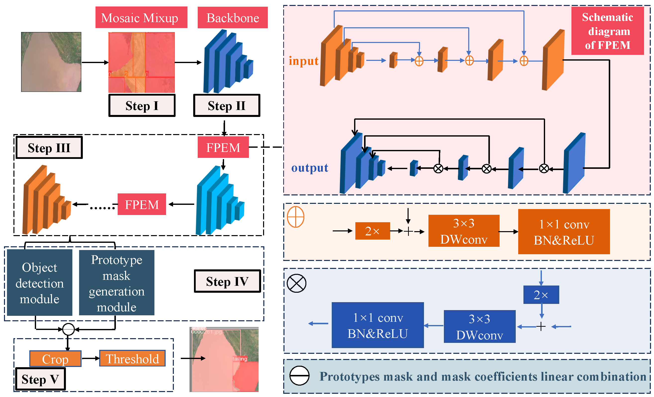
2.2.1. Optimized YOLACT Model

The You Only Look At CoefficienTs (YOLACT) model, developed by the University of California [34], is a streamlined, fully convolutional network designed for real-time instance segmentation. It demonstrated a mean Average Precision (mAP) of 29.8 on the MS COCO dataset, achieving processing speeds of 33.5 frames per second on a single Titan Xp GPU. This rate of performance is significantly faster than many prior competitive methods. To further improve the detection capabilities of the YOLACT model for tailings pond BLIs observation, this study introduces the following optimizations.

Optimization I: The original loss function, Intersection over Union (IoU), is revised to Generalized IoU (GIoU). The traditional IoU loss function results in a zero loss when the predicted bounding box does not intersect with the actual box, thereby providing no gradient for training and hindering the neural network’s learning progression. GIoU rectifies this by integrating the concept of the smallest enclosing rectangle that encompasses both the predicted and actual bounding boxes. This optimization not only resolves the issue of vanishing gradients in cases of non-overlapping boxes but also boosts the accuracy and response speed of the model.

$$IOU={\displaystyle \frac{\left|A\cap B\right|}{\left|A\cup B\right|}}$$

(1)

$$lossIOU=1-IOU$$

(2)

$$GIOU=IOU-{\displaystyle \frac{\left|C-A\cap B\right|}{\left|C\right|}}$$

(3)

Here, A refers to the predicted bounding box, representing the dimensions and position of the predicted area. B denotes the true bounding box, indicating the actual measured area. And C is the smallest rectangle covering both A and B.

Optimization II: The original Feature Pyramid Network (FPN), used for feature extraction, has been supplanted by an advanced Feature Pyramid Extraction Module (FPEM). The FPEM integrates cascading modules that enhance feature amalgamation across varied scales, substantially enlarging the feature receptive field. It also employs distinct, computationally efficient convolutions. This novel configuration decreases the computational load to approximately one-fifth of the original FPN demands [35].

Optimization III: A novel data augmentation technique, termed Mosaic Mixup, has been incorporated to bolster the model’s robustness. This approach enhances the robustness by cropping and stitching images, thus effectively expanding the training dataset.

The workflow of the optimized YOLACT model is delineated in Figure 2 and involves the following steps. Step I: The dataset is input into the Mosaic Mixup data augmentation module to amplify data diversity. Step II: The enhanced dataset is then fed into the backbone network, which performs the initial feature extraction. Step III: The FPEM is utilized to amalgamate multiscale features derived from the backbone network. Step IV: The process splits into two parallel task branches. One branch is tasked with generating a prototype mask that encapsulates the entire image. The other branch undertakes object detection, calculating candidate bounding box confidence scores, anchor box positions, and mask coefficients. Step V: Matrix multiplication is applied between the prototype masks and mask coefficients to construct instance masks for the actual objects in the image. Masks that do not pertain to the tailings category are excised beyond the boundary to refine and clarify the boundary image. These steps elucidate the comprehensive procedures in the optimized YOLACT model’s data processing and feature extraction phases, underscoring substantial advancements in segmentation accuracy and processing efficiency.

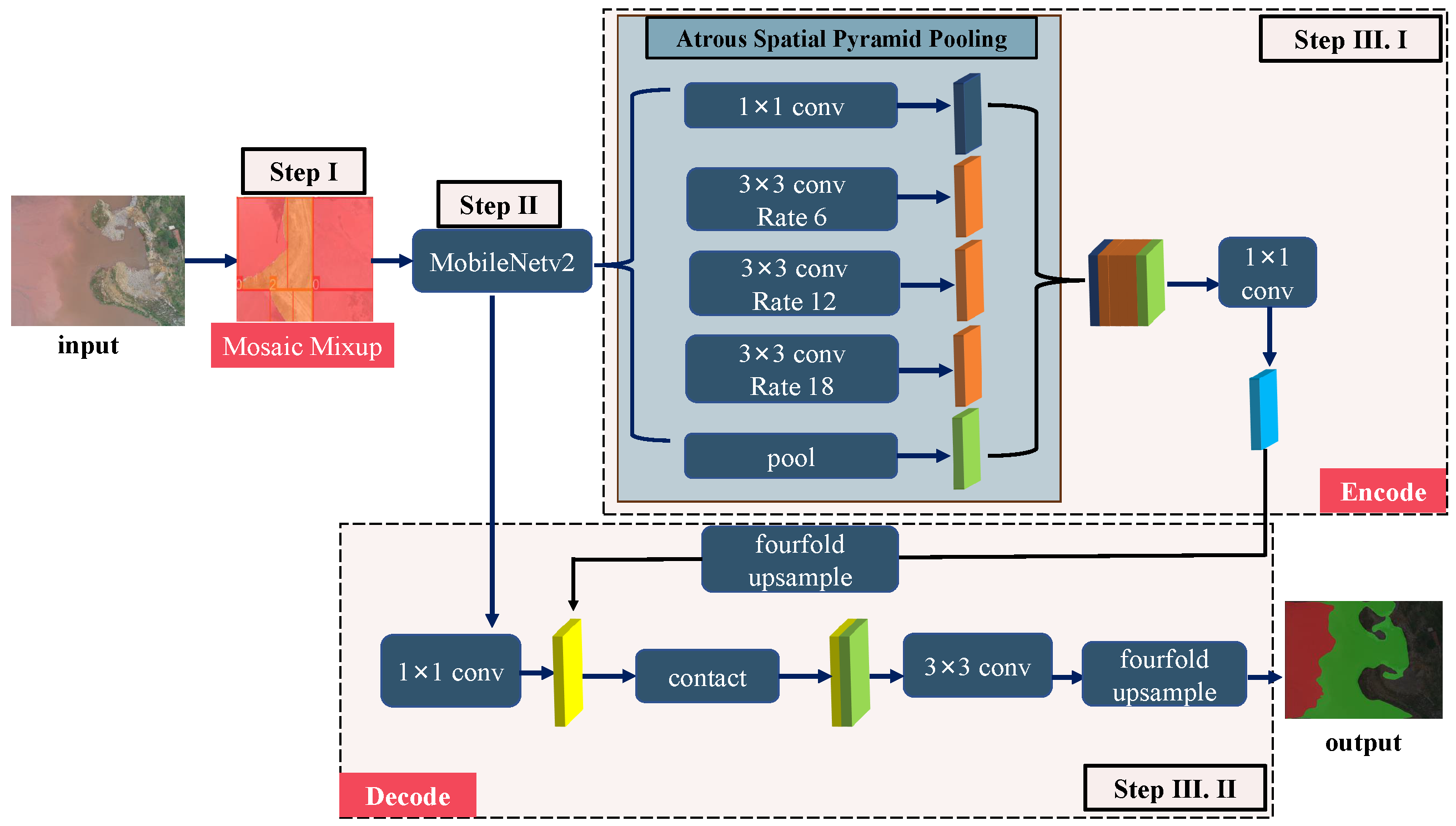
2.2.2. Optimized DeepLabV3+ Model

The DeepLabV3+ model, a state-of-the-art semantic segmentation framework developed by Google [36], has been subjected the following optimizations to enhance its computation speed and robustness.

Optimization I: The original backbone network, Xception, has been supplanted by MobileNetv2. This modification preserves the model’s accuracy while considerably reducing its computational complexity, rendering it more suitable for applications with limited resource availability.

Optimization II: Data augmentation techniques, notably Mosaic Mixup, have been integrated to enrich the training dataset. This expansion enhances the model’s robustness, enabling it to more effectively handle diverse input scenarios.

The architecture of the DeepLabV3+ model comprises distinct encoding and decoding components. The model’s workflow, illustrated in Figure 3, includes the following steps.

Step I: The dataset undergoes data augmentation via Mosaic Mixup, enhancing the variety and complexity of the training data.

Step II: Images are processed through the MobileNetv2 backbone network for feature extraction. This network generates two layers of features—one deep and one shallow—capturing different levels of semantic information that are crucial for nuanced image understanding.

Step III.I: The deep features are channeled into the Atrous Spatial Pyramid Pooling (ASPP) module. This innovative module is equipped with one 1 × 1 convolution and three atrous convolutions with dilation rates of 6, 12, and 18, alongside a global average pooling layer. The collected features from these operations are concatenated and subjected to an additional 1 × 1 convolution to standardize the feature channels, preparing them for subsequent processing stages.

Step III.II: During the decoding phase, the shallow features are refined using a 1 × 1 convolution to enhance the feature map clarity. These refined features are amalgamated with the concatenated deep features from the encoding stage. Following this integration, a 3 × 3 convolution is applied to bolster feature integration. The resulting data are then upsampled to the original image dimensions, enabling precise pixel-level predictions for classifying each pixel, thereby culminating the segmentation process.

2.3. Tailings Dam Stability Evaluation Methods

The safety factor for the anti-sliding stability of tailings dam slopes is defined as the ratio of the resistance against sliding along a presumed sliding surface to the sliding force. The current Tailings Dam Safety Regulations of China recommend employing simplified methodologies such as the Bishop method for these calculations. The anti-sliding stability for both initial and accumulated dams is evaluated based on the physical and mechanical characteristics of the dam materials and their foundations.

In this study, the simplified Bishop method is used to calculate the two-dimensional (2D) slope stability. It is based on the principle of limit equilibrium, assuming a circular sliding surface and discretizing this surface into individual soil strips. It considers the normal forces between these strips while omitting the tangential forces, thus simplifying the computation of the slope stability coefficient. The stability coefficient is defined as the ratio of the maximum resisting moment to the maximum driving moment. The formula for iterative calculations in the simplified Bishop method is as follows:

$$K={\displaystyle \frac{{\sum }_{i=1}^n\frac{1}{m_{ai}}\left(c_i{b}_{i}cos{\alpha }_i+W_{i}tan{\phi }_i\right)}{{\sum }_{i=1}^n{W}_{i}sin{\alpha }_i}}$$

(4)

$$m_{ai}=cos{\alpha }_i+{\displaystyle \frac{sin{\alpha }_{i}tan{\phi }_i}{K}}$$

(5)

Here, K denotes the stability coefficient. $W_i$ is the weight of the soil strips (kg). $c_i$ represents the cohesion (kN). ${\phi }_i$ is the internal friction angle (°). ${\alpha }_i$ refers to the normal angle (°). And $b_i$ indicates the sliding surface length (m).

For 3D slope stability, the Strength Reduction Method (SRM) [37] is utilized. The SRM involves diminishing the shear strength parameters (c, $\phi$) of the rock and soil mass using reduction factors. The stability analysis is conducted following these adjustments. The reduction factors are incrementally increased through iteration until a critical failure state is achieved. The corresponding reduction factor at which the failure occurs is designated as the safety factor.

$$c_m={\displaystyle \frac{c}{F_{\tau }}}$$

(6)

$${\phi }_m=\arctan \left(\tan \phi /F_{\tau }\right)$$

(7)

Here, c and $\phi$ represent the original cohesion (kPa) and internal friction angle (°), respectively. $c_m$ and ${\phi }_m$ denote the reduced cohesion (kPa) and friction angle (°). And $F_{\tau }$ signifies the reduction factor.

Importantly, the numerical model construction and condition setting have a decisive influence on the safety evaluation outcomes. Despite this, common engineering practices often default to using either design-based conditions or monitor a minimal beach width to model the initial water level conditions, employing simplified 2D or pseudo-three-dimensional (P-3D) models. The reliability of these approaches warrants further examination.

2.4. Tailings Pond Seepage Evaluation Method

Tailings pond seepage evaluation is also required by regulations to assess their operational safety, helping to ascertain both stability and environmental risks associated with potential seepage during design and operational phases [38]. Reliable seepage modeling requires understanding how water migrates through tailings, whether in a saturated or unsaturated state, governed by Darcy’s Law. This law states that water flow through a porous medium is proportional to the hydraulic gradient.

The mathematical framework for seepage under steady-state conditions in three dimensions is captured by the following differential equation:

$${\displaystyle \frac{\partial }{{\partial }_x}}\left(k_x{\displaystyle \frac{\partial }{{\partial }_x}}\right)+{\displaystyle \frac{\partial }{{\partial }_y}}\left(k_y{\displaystyle \frac{\partial }{{\partial }_y}}\right)+{\displaystyle \frac{\partial }{{\partial }_z}}\left(k_z{\displaystyle \frac{\partial }{{\partial }_z}}\right)=0$$

(8)

For unsteady seepage, the differential equation is expanded to include time dependence:

$${\displaystyle \frac{\partial }{\partial x}}\left(k_x{\displaystyle \frac{\partial }{\partial x}}\right)+{\displaystyle \frac{\partial }{\partial y}}\left(k_y{\displaystyle \frac{\partial h}{\partial y}}\right)+{\displaystyle \frac{\partial }{\partial z}}\left(k_z{\displaystyle \frac{\partial h}{\partial z}}\right)={\mathrm{S}}_{\mathrm{s}}{\displaystyle \frac{\partial h}{\partial t}}$$

(9)

Here, h represents the hydraulic head function, $k_x$, $k_y$, and $k_z$ denote the permeability coefficients along the respective axes, and $S_S$ is the specific storage coefficient.

The boundary conditions for modeling 3D steady-state seepage under varied physical scenarios are classified into three types.

The first type ${\mathsf{\Gamma }}_1$ represents known boundary heads. The second type ${\mathsf{\Gamma }}_2$ represents impermeable or zero-flux boundaries. The third type ${\mathsf{\Gamma }}_3$ represents boundaries with rainfall infiltration:

$$h|{\mathsf{\Gamma }}_1=h\left(x,y,z\right)$$

(10)

$$k_x{\displaystyle \frac{\partial h}{\partial x}}cos\left(n,x\right)+k_y{\displaystyle \frac{\partial h}{\partial y}}cos\left(n,y\right)+k_z{\displaystyle \frac{\partial h}{\partial z}}cos\left(n,z\right)|{\mathsf{\Gamma }}_2\ge 0$$

(11)

$$k_{rx}{\displaystyle \frac{\partial h}{\partial x}}cos\left(n,x\right)+k_{ry}{\displaystyle \frac{\partial h}{\partial y}}cos\left(n,y\right)+k_{rz}{\displaystyle \frac{\partial h}{\partial z}}\cos \left(n,z\right)|{\mathsf{\Gamma }}_3=q_n$$

(12)

Here, $h(x,y,z)$ is the known pressure head, and n is the outward normal at ${\mathsf{\Gamma }}_2$. $k_{rx}$, $k_{ry}$, and $k_{rz}$ are the relative permeabilities in the x, y, and z directions. And $q_n$ is the infiltration flow rate.

Finite Element Analysis (FEA) is employed to tackle these boundary conditions within a numerical setup effectively. FEA utilizes the variational principle to equivalently transform the boundary value problem presented by the seepage differential equation, enabling the determination of the hydraulic head at each nodal element in the mesh.

3. Case Study

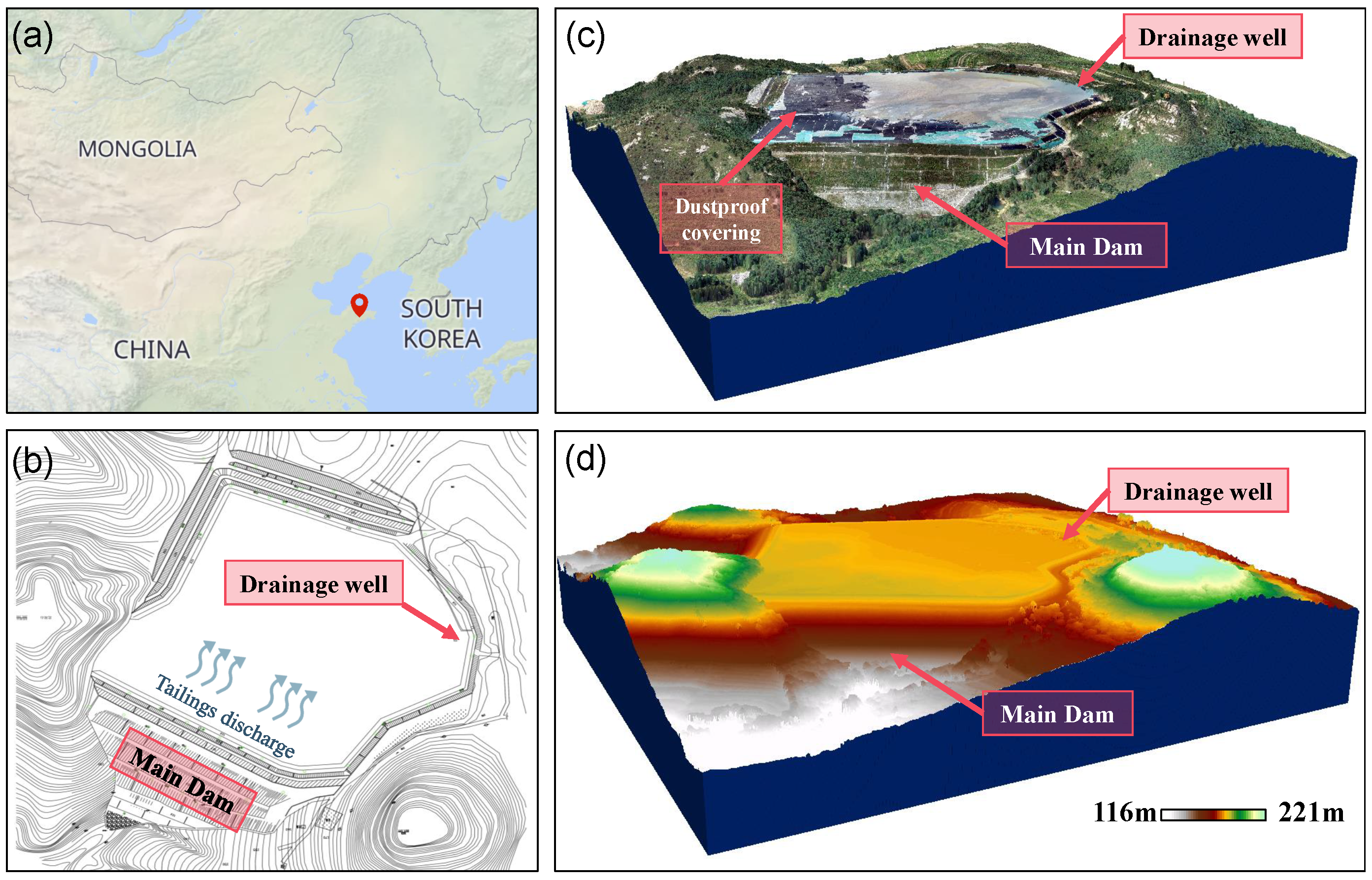
3.1. Engineering Background

The tailings pond in the case study is situated in Shandong Province, which is the leading gold-producing region in China, with an annual output exceeding 140 tons. The starter dam is designed with a height of 12 m and an outer slope ratio of 1:2. It is constructed as a rolled stone dam with anti-filtration measures implemented on the inner slope to enhance safety. The embankments, constructed using the economical but less safe upstream method, have a height of 3 m each, an outer slope ratio of 1:2.5, and a top width of 4.5 m. The dam, reaching a total height of 54 m, has a final storage capacity of $2.021\times {10}^6$ m³.

The flood discharge system comprises a drainage well, drainage culverts, and a water recovery system. Beach width monitoring is performed by measuring the embankment crest elevation and decant water level via radar level gauges—based on the assumption of a constant beach slope.

The DJI Matrice 350 RTK quadcopter drone equipped with a Zenmuse P1 full-frame camera was used in this study. The surveying was executed with flight routes arranged in a “cross” pattern to optimize coverage. The planned heading and lateral overlaps were 70% and 80%, respectively, at a flight altitude of 120 m, achieving a Ground Sampling Distance (GSD) of 1.5 cm/pixel. A total of 1739 images were collected. These images were then processed to produce a high-resolution DOM and DSM, as presented in Figure 4.

The two-dimensional (2D), pseudo-three-dimensional (P-3D) and real three-dimensional (R-3D) models were constructed, as shown in Figure 5, based on the engineering background of the case study. The minimum beach width and the CNN’s automatically identified BLIs were used as the input parameters to facilitate comparative analyses of the dam anti-sliding stability. The physical and mechanical properties of the geotechnical layers within the tailings pond are outlined in

Table 1. Parameters of physical and mechanical properties of the geotechnical layers.

Geotechnical Material	Unit Weight $\mathit{\gamma }$ (kN/m3)	Cohesion C (kPa)	Internal Friction Angle Φ (°)	Permeability Coefficient K (m/s)
Foundation
Highly Weathered Granite	22	0	41	-
Starter dam
Compacted Rolled Stone Dam	21	0	36	$1.0\times {10}^{-3}$
Upstream embankments
Compacted Soil and Rock Dam	20.5	1	37	$3.5\times {10}^{-5}$
Tailings Layer
Tailings Sand	19.2	6.4	30	$5.5\times {10}^{-7}$
Tailings Soil	18.5	13.7	26.4	$5.09\times {10}^{-7}$

.

3.2. Research Procedure

(1) UAV Survey

The DOM and DSM of the tailings pond and its surrounding environment are generated from UAV surveys and photogrammetry processing.

(2) Dataset Preparation

A dataset comprising 600 images of tailings ponds is assembled using ArcGIS 10.2 software. Then, the dataset is expanded to 6000 images using the Mosaic Mixup data augmentation module. These images are meticulously annotated using precise tools to ensure accurate labeling. The dataset is divided into training (90%) and testing (10%) subsets to facilitate the development and validation of CNN models.

(3) Model Training and Evaluation

The optimized YOLACT and DeepLabV3+ models are trained separately with the prepared dataset to extract beach and water areas. The performance of these models is evaluated and compared against manual annotated results to ascertain the more effective model.

(4) Beach Boundary Line Extraction

Deploy the identified superior CNN model to extract the boundary line between the beach and decant pond from the UAVP-generated DOM.

(5) Beach Width Measurement

The distance between the water boundary and the embankment crest is determined by connected component extraction using MATLAB R2018b software. It is then converted into actual measurement by scaling with the grid pixel size to determine the shortest beach width.

(6) Beach Slope Measurement

Beach slopes are determined based on the elevation changes observed in multiple profiles drawn on the DSM. The average beach slope is then calculated.

(7) Tailings Dam Stability and Seepage Evaluation

Based on the DSM data and the extracted BLIs, three comparative tailings dam stability evaluation models are developed. Model A (2D model): Utilize the minimum beach width as the water level condition, as shown in Figure 5a. Model B (P-3D model): Extend the 2D profiles fitting with the water level condition, as shown in Figure 5b. Model C (R-3D model): Using the UAVP-generated DSM and the extracted water level condition, as shown in Figure 5c. Then, compare and analyze the outcomes of dam stability and seepage analyses delivered by these models.

3.3. Model Training and Recognition Results

The mean Intersection over Union (MIoU) and mean Pixel Accuracy (mPA) serve as pivotal quantitative metrics for evaluating segmentation models. The MIoU quantifies the overlap between the predicted and true labels as a ratio of their intersection to the union, while the mPA calculates the average pixel accuracy across each categorically identified segment. A higher MIoU indicates better model accuracy, and a higher mPA reflects greater precision. Employing these metrics, the optimized DeepLabV3+ model achieved an MIoU of 63.41% and an mPA of 67.3%. Despite these metrics, the model’s generalization capabilities remain constrained. As illustrated in Figure 6a1,a2, the tailings pond UAV images exhibit low color contrast between the beach and water, posing challenges in boundary delineation. In its prediction phase, DeepLabV3+ utilizes bilinear upsampling of feature maps by a factor of 16, which could result in the loss of critical detail and negatively impact the accuracy of recognition.

Conversely, the optimized YOLACT model demonstrated enhanced performance, achieving an MIoU of 72.63% and an mPA of 76.2%. This model incorporates an FPEM structure that adeptly fuses feature maps from various scales, significantly expanding the receptive field. This design ameliorates the detail loss associated with downsampling and boosts the model’s overall recognition capability.

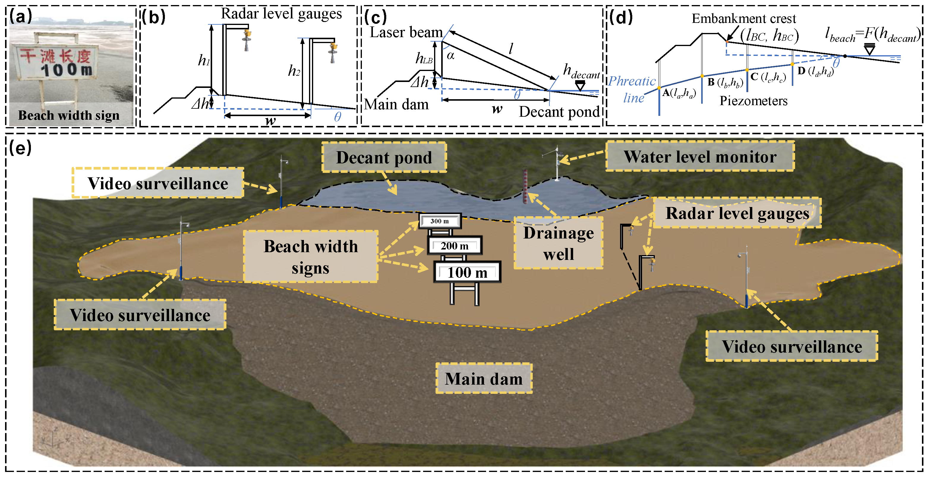
3.4. Measurement of Beach Width and Slope

Utilizing the optimized YOLACT model, the contours delineating the beach interface and the boundary edge of the decant pond were extracted from the UAVP-generated DOM, as shown in Figure 7. The methodology for automatically determining the minimum beach width involves a series of raster computations. Initially, the high-resolution orthophoto is aligned with the DSM, restoring the positional accuracy lost during the image recognition phase. This aligned image is then subjected to binary classification. Areas representing waterlines and dam lines are assigned a binary value of 0 (black), while all other regions are set to 1 (white). Connected component analysis is applied to identify and categorize the grids associated with the waterlines and dam lines. Through iterative analysis of these categories, the minimum distance between these features was calculated to be 127.53 m. Recording the Z coordinates of the endpoints at this distance, the shortest linear distance is then scaled by the pixel size of 1.5. By incorporating this calculation with the elevation data, the spatial shortest beach width was computed to be 191.31 m.

Observations of the beach slope must be arranged with at least two sections every 100 m, and the spacing between measurement points should not exceed 10∼20 m according to the current Chinese technical regulations for the tailings pond safey monitoring. The UAVP-generated DSM can be used to extract elevation measurements for any section, offering a more efficient coverage compared to the observational methods previously discussed. With the main dam length measured at 270 m, six sections were established in accordance with the specifications, with each approximately 45 m apart, as shown in Figure 8a. These sections were then aligned with the DSM to extract the 3D coordinates of the line segments for subsequent slope calculations. The beach slope variations from section I to section VI, plotted in Figure 8b–g, demonstrate average slopes of 1.5%, 1.4%, 1.2%, 1.5%, 1.3%, and 1.6% respectively. Consequently, the calculated average beach slope for the tailings pond was determined to be 1.42%.

3.5. Tailings Dam Stability Evaluation Results

The results of tailings dam stability evaluation are presented in Figure 9, showcasing corresponding dam stability coefficients of 2.096, 3.10, 3.86, and 4.00.

The dam stability coefficient, determined using the 2D simplified Bishop method, came out to 2.096 (Figure 9a), surpassing the safety threshold mandated by current Chinese regulations, which stipulate a minimum safety factor of 1.25 for the fourth-class tailings dams in the case study. The potential sliding surface was identified within the central segment of the dam embankment, spanning an area of 228.1 m². The dam stability coefficient determined using the 2D SRM method was 3.10 (Figure 9b), indicating a 47.9% increase compared to the Bishop method. The identified potential sliding surface extends from the embankment crest to the initial dam crest, primarily located in the lower central portion, encompassing an area of 226.4 m². The stability coefficient calculated using the P-3D SRM method was 3.86 (Figure 9c), demonstrating a 24.5% increase compared to the 2D SRM method. The peak shear stress was distributed similar to the 2D SRM calculation, covering an area of 249.1 m², with a stress distribution from 83 to 200 kPa. The stability coefficient obtained from the R-3D SRM method was 4.00. Analysis of shear stress distribution along a profile perpendicular to the main dam axis reveals the primary potential sliding surface situated at the embankment’s center, with an associated potential sliding area of 230.6 m². Shear stress on the potential sliding surface varied from 117 to 183 kPa, suggesting correlation with factors such as dam geometry, beach width, and water level conditions.

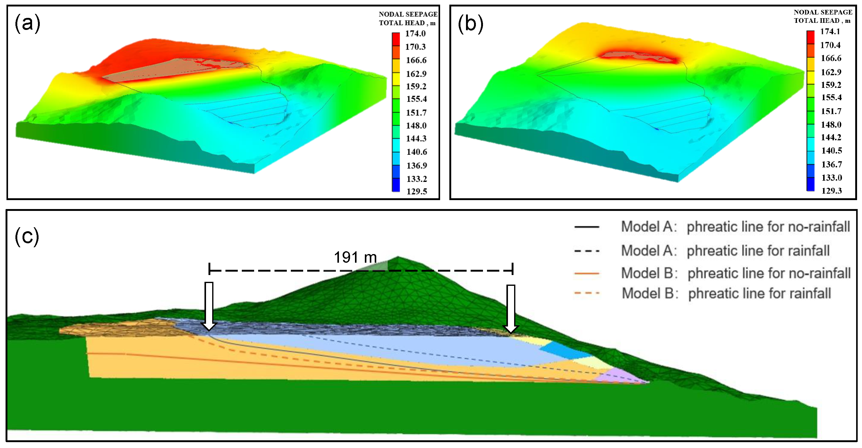
3.6. Tailings Pond Seepage Evaluation Results

This study investigates the impact of defining the beach boundary line, specifically the water level line of the decant pond, on tailings pond 3D seepage calculations. Based on the case study, the research conducted 3D seepage predictions under the scenario of 24 h rainfall, totaling 50 mm. Two comparive 3D seepage calculation models were established based on the UAVP-generated DSM. These models were initialized with water levels set at the minimum beach width condition (Model A) and the actual beach boundary line condition, as depicted in Figure 7 extracted by the optimized YOLACT (Model B).

The computational results are illustrated in Figure 10, indicating that the peak total head value for Model A occurred upstream of the shortest beach line, exhibiting a uniform, gradual decrease perpendicular to the dam axis downstream. Conversely, for Model B, the peak total head value was situated at the decant pond, gradually decreasing downstream along the accurately extracted beach boundary. These variations stem from the disparate initial water level conditions. Figure 10c demonstrates the phreatic line variations along the section perpendicular to the main dam axis under both rainfall and non-rainfall conditions. In the absence of rainfall, noticeable differences in the phreatic line depth between Models A and B were observed. Model A’s phreatic line reached a position 191 m directly from the dam crest, whereas in Model B, the phreatic line did not reach the beach surface in the shown section. During rainfall conditions, Model B’s predicted phreatic line was lower than that of Model A, even surpassing Model A’s phreatic line under non-rainfall conditions.

The phreatic line is a critical indicator for assessing the safety of tailings ponds. Tailings particles below the phreatic line are in a saturated state. When the phreatic line rises, the shear strength of the tailings material decreases due to the effect of seepage water, reducing the sliding resistance of the slope and increasing the sliding force, thereby leading to a decline in stability. Wang et al. [39] demonstrated that a 1-m increase in the phreatic line height can result in a stability decrease of 0.05 or more. According to the Chinese ”Safety Regulations for Tailings Ponds” (GB 39496-2020) [40], for tailings dams with heights below 30 m, the phreatic line depth should be maintained at more than 2 m. The central cross-section of the dam as a typical profile was selected for analysis. In Models A and B, under both non-rainfall and rainfall conditions, the maximum depths of the phreatic line were 8.66, 4.55, 8.67, and 8.66 m, respectively, which comply with safety regulations. The Model B results indicate higher seepage stability, while the Model A results are more conservative.

4. Discussion

4.1. CNN Models Identification Performances and Future Improvements

Comparative analyses reveal that the YOLACT model, with its advanced feature integration strategy, substantially outperformed DeepLabV3+ in the segmentation of the tailings beach and decant pond. These findings underscore the YOLACT model’s superior ability to manage the intricate segmentation tasks essential for the accurate delineation of environmental scenes, such as those encountered in monitoring tailings ponds. However, due to the scarcity of available data, the training dataset primarily consists of satellite and UAV imagery obtained from iron or gold tailings ponds. Tailings ponds manifest diverse reflection image characteristics influenced by various factors such as the ore type, weather conditions, lighting conditions, and optical sensors [41]. To mitigate this variability, we propose the creation of tailored image training sets specific to the individual tailings ponds designated for UAV surveillance. This strategy is intended to optimize the CNNs’ performance in identifying and delineating BLIs. Moreover, the integration of multispectral, InSAR, or other multisource remote sensing data can enrich the information sources for BLIs monitoring [42,43].

Compared to conventional methods shown in Figure 1, the proposed approach delineated the boundary line between the decant pond and the beach in a “planar” format rather than a “line measurement” format. This transition could increase the data density by one dimension. The “planar” format enables more reliable calculation of the minimum beach width. Additionally, the actual beach area extracted provides crucial inputs for constructing more accurate numerical models for dam stability and seepage calculations, thereby enhancing the reliability of safety evaluation.

In terms of analyzing the beach slope, this method allows for the extraction of elevation data from any desired section on the DSM data, offering greater flexibility in calculating beach slope. It generated high-resolution slope variation curves, as illustrated in Figure 8, which more precisely depict the true undulations of the beach surface.

Looking forward, integrating the proposed approach with automatic charging and data transmission UAV station technology could significantly advance the autonomous collection of comprehensive monitoring data. The beach area, dam height, dam cracks, subsidence, storage capacity, and surrounding environment of the tailings pond can be obtained by UAVs [44,45,46]. These advancements would not only enhance the intelligence and observational capabilities, but they would also reduce manual work intensity within tailings management practices.

4.2. Impacts of Model Geometry on Tailings Dam Stability Evaluation

The R-3D model depicted the tailings dam body’s geometry as an inverted trapezoid, with significant shear stress concentration observed at the trapezoidal long base’s midpoint. In contrast, shear stress on the lateral sides, corresponding to the dam abutments, were comparatively lower. This disparity underscores the necessity of employing R-3D modeling techniques in dam safety coefficient calculations. As Wu et al. [47,48] demonstrated in the field of landslide research that the three-dimensional geometric shape of the dam body has a significant impact on the stability analysis results. Furthermore, tailings dams, often constructed in valleys, may have their stability analysis results influenced by the surrounding valley geometry [49]. These factors underscore the importance of conducting 3D dam stability analysis based on UAV aerial surveys.

The simplified Bishop method solely accounts for inter-slice normal forces—fulfilling vertical force balance and overall moment equilibrium—and its computational process is relatively straightforward, thus making it widely applicable in engineering practices [50]. In contrast, the SRM comprehensively addresses static equilibrium, strain compatibility, and the non-linear stress–strain relationship of soil masses. Its application extends to calculating dams with complex topography and geology, unrestricted by dam geometry, boundary conditions, or material heterogeneity. When determining safety factors, there is no need to assume the potential sliding surface or perform slice divisions. Instead, the program automatically determines the sliding surface, locating sliding failure within regions characterized by shear strain increments, plastic strains, or abrupt displacement changes [51,52].

The 2D computational approach demonstrates significant efficiency, facilitating seamless integration with online safety monitoring systems by incorporating variables such as water level monitoring, thus enabling real-time dynamic assessment of tailings dam stability coefficients. It is crucial to acknowledge that 2D methods may potentially underestimate actual dam stability and are most suitable for dams characterized by regular geometries and uniform geological conditions [53]. The P-3D method partially incorporates 3D effects and is particularly suitable for stability analyses characterized by significant length-to-height ratios. Despite the prolonged duration required for establishing 3D stability calculations using the SRM, the computational duration remained about 10 min, wherein the time investment is fully justifiable for engineering design assessments or validating alterations at this magnitude. Furthermore, the rapid advancement of high-performance computing devices is anticipated to mitigate any adverse effects on computational efficiency associated with 3D calculations. Addressing the complexity and non-linearity inherent in dam stability evaluation, Fu et al. [54] have introduced a method leveraging big data and CNNs. This approach utilizes actual and synthetic dam slope data to provide generate training and testing samples for CNNs, enhancing the speed and applicability of CNN-based assessments in practical engineering.

4.3. Impact of Discrepancies in Dam Stability Results on Decision Making

In terms of stability coefficient reliability, Brown and Gillani [55] have identified frequent errors in tailings dam stability evaluation, which can lead to significant overestimations or underestimations of safety coefficients, potentially masking real risks or resulting in overly conservative designs. Ferreira de Souza [56] noted that a 10% variation in dam stability evaluation can significantly influence design acceptance criteria, advocating for a cautious application of stability calculation methods and recommending the use of multiple methods for cross-validation.

According to the case study, employing the 2D SRM for dam stability calculations yielded 24.5% higher stability coefficient results compared to the simplified Bishop method. And the R-3D SRM delivered a stability coefficient that is 29% and 3.63% higher than the 2D SRM modeling. This disparity implies that the simplified 2D calculations may underestimate dam stability due to model simplification [53]. This variation reflects the actual morphology of the tailings dam area, dam body geometry, surrounding environment, as well as the configurations of beach line boundaries, all of which significantly impact dam stability calculations [57,58,59].

Higher stability coefficients could mitigate regulatory pressures on mining companies while reducing the margin of error in safety evaluation. Regulatory authorities should strive to balance setting minimum stability coefficients that ensure adequate error margins while promoting sustainable mining approaches. Excessively stringent regulations may force companies to overinvest in dam construction, heightening construction difficulties and unsustainable costs, which could detract from investments in safety operations, monitoring system maintenance, and environmental protection, ultimately undermining the overall safety management of tailings ponds.

The approach of 3D numerical analysis is recommended for complex terrains and dam shapes, variable geological conditions, and tailings ponds that pose significant potential disaster risks. It is advisable to conduct UAVP 3D modeling and numerical calculations and to perform staged dam stability analyses following each embankment completion. Moreover, employing various stability evaluation methods for cross-validation and conducting parameter sensitivity analysis are crucial to ensuring both the safety and economic viability of tailings pond designs [60].

This study underscores the importance of BLIs UAV observation and topographic parameters in validating and calibrating numerical models. By integrating actual monitoring data with advanced calculation methods such as the SRM, the dam stability can be more accurately assessed, providing a scientific basis for the design and safety management of tailings ponds.

4.4. Impacts of Model Geometry and Water Level Conditions on Seepage Simulation

The phreatic line, often metaphorically described as the “lifeline” of a tailings pond, marks the highest level within the dam body where water seeps or percolates. This line effectively delineates the saturated zone, which is characterized by tailings pores fully filled with water, from the unsaturated zone above, which contains both air and water within the tailings pores. A lower phreatic line signifies reduced water pressure within the dam, decreasing both the likelihood and intensity of seepage through the dam body. Consequently, with a lower phreatic line, the section of the dam above this line experiences less saturation, enhancing its stability [33,61]. The phreatic line is primarily determined through sensor measurements of pore water pressure, as illustrated in Figure 1d. Predicting the phreatic line depth under rainfall conditions through numerical seepage simulation is an essential part of the safety evaluation and validation process for tailings facilities [62].

The 3D numerical seepage simulation results highlight the critical role of model geometry and water level condition setup. Simplified water level conditions may underestimate the seepage stability under rainfall conditions due to the unique geometries of each tailings pond, thereby imposing undue burdens on operational and safety oversight.

Frequent false alarms can erode the credibility of tailings pond safety monitoring and early warning systems, increase unnecessary workloads and emergency response costs, and lessen the vigilance and responsiveness of management personnel [63]. In this case study, the modeling calculations based on actual waterline conditions observed using the optimized YOLACT model are more conservative and recommended for onsite 3D seepage evaluation. This method helps reduce false alarms, streamline superfluous safety management expenditures, and enhance the reliability and effectiveness of tailings safety management.

Furthermore, the duration of 3D seepage calculations depends on model complexity and computing hardware capabilities. The current simulation required 3915 s and could predict phreatic line parameters 24 h after potential rainfall events. Incorporating the proposed automated BLI extraction method, it is expected to facilitate more robust 3D seepage evaluation and strengthen the credibility of safety forecasts and early warning mechanisms during rainfall events.

5. Conclusions

This study utilized a UAVP to generate a DOM and DSM of a tailings pond and its surrounding environment. CNNs were used for the automated identification of tailings pond BLIs. Significant enhancements were implemented to optimize the YOLACT model, including the adoption of the GIoU to improve accuracy in scenarios where bounding boxes do not overlap and an advanced FPEM that replaced the original FPN, reducing computational demands and enhancing feature integration across scales. For the DeepLabV3+ model, the backbone network was upgraded to MobileNetv2 to decrease computational complexity while retaining accuracy, and Mosaic Mixup data augmentation was implemented to boost robustness and effectiveness in handling varied inputs. The performance outcomes of the optimized YOLACT and DeepLabV3+ models were then evaluated. The minimum beach width was extracted using raster computation to ascertain it. And the beach slope was determined by extracting elevation profiles from the DSM raster. Finally, comparative analyses highlighted the advantages of constructing a R-3D model over commonly used 2D or P-3D models for the tailings dam anti-sliding stability and 3D seepage calculations. The proposed approach enables the reproduction of complex geometries and heterogeneous material properties of the dam structure, which is crucial for ensuring the safety and economic efficiency of tailings pond designs.

The main conclusions are as follows:

(1) Compared to the optimized DeepLabV3+ model, the optimized YOLACT model more effectively identified the boundaries between tailings beach and decant pond water, achieving an mIoU value of 72.63% and an mPA value of 76.2%.This approach, leveraging UAVP and CNNs, holds promise for future integration with automated charging and data transmission UAV station technology, thereby enhancing the dynamic observation of beach width and slope for more reliable tailings pond safety monitoring.

(2) The anti-slide stability of tailings dams can exhibit disparities contingent upon geometric restitution and water level condition configurations. The case study suggests that 2D calculations using the simplified Bishop method and minimal beach width conditions may incline towards understimating the dam stability. Conversely, 3D numerical modeling, enhanced by actual BLIs conditions extracted from the proposed approach, proves suitable for stability evaluation of critical tailings dams, which often feature complex terrain, varied dam body geometries, diverse geological conditions, and a heightened potential for severe disaster consequences.

(3) The configuration of the water level condition, particularly the beach width parameter, significantly impacted the outcomes of 3D seepage simulations. Results based on actual waterline conditions extracted by the optimized YOLACT model are more conservative and, therefore, recommended for onsite seepage evaluation in engineering practices. These methods help diminish the frequency of false alarms and are anticipated to bolster the credibility of early warning alerts.

(4) With the trend of large-scale fine tailings outputs and embankment construction, the paramount objective should be to realize the tailings management vision of zero harm to people and the environment. This necessitates advancing beyond existing tailings dam safety management practices by deploying various safety monitoring devices, including UAVs, employing multiple safety assessment calculation methods for cross-validation, and conducting parameter sensitivity analysis studies. Regulatory authorities must establish standards and regulations based on scientific evidence to avoid overestimating or underestimating the stability of tailings dams, thereby ensuring the promotion of safety and sustainable tailings pond designs.

References

1. Cornwall, W. A dam big problem. Science 2020, 369, 906–909. [Google Scholar] [CrossRef] [PubMed]
2. Wu, F.; Liu, Y.; Qu, G.; Xie, R. High value-added resource treatment of antimony tailings: Preparation of high-strength lightweight foam concrete materials. Process Saf. Environ. Prot. 2022, 166, 269–278. [Google Scholar] [CrossRef]
3. Aswathi, T.S.; Jakka, R.S. Seismic analysis of hybrid tailings dams: Insights into stability and responses. Bull. Eng. Geol. Environ. 2024, 83, 56. [Google Scholar] [CrossRef]
4. Ma, C.; Guo, X.; Yang, C.; Zhang, C.; Ma, L.; Li, X. Velocity field and outflow discharge behavior in overtopping dam-break of an iron mine tailings dam: A model test. Bull. Eng. Geol. Environ. 2024, 83. [Google Scholar] [CrossRef]
5. WISE Uranium Project. Chronology of Major Tailings Dam Failures. Available online: https://www.wise-uranium.org/mdaf.html (accessed on 5 February 2024).
6. Islam, K.; Murakami, S. Global-scale impact analysis of mine tailings dam failures: 1915–2020. Glob. Environ. Chang.-Hum. Policy Dimens. 2021, 70, 102361. [Google Scholar] [CrossRef]
7. Hudson-Edwards, K.A.; Kemp, D.; Torres-Cruz, L.A.; Macklin, M.G.; Brewer, P.A.; Owen, J.R.; Franks, D.M.; Marquis, E.; Thomas, C.J. Tailings storage facilities, failures and disaster risk. Nat. Rev. Earth Environ. 2024, 1–19. [Google Scholar] [CrossRef]
8. Chen, Y.; Jing, X.; Wei, Z.; Wang, M. Physical and numerical modeling of the hypothetical tailings dam breach runout and mitigation with a slurry-resisting barrier. Bull. Eng. Geol. Environ. 2023, 82, 265. [Google Scholar] [CrossRef]
9. Zhuang, Y.; Jin, K.; Cheng, Q.; Xing, A.; Luo, H. Experimental and numerical investigations of a catastrophic tailings dam break in Daye, Hubei, China. Bull. Eng. Geol. Environ. 2022, 81, 9. [Google Scholar] [CrossRef]
10. Clarkson, L.; Williams, D. Critical review of tailings dam monitoring best practice. Int. J. Mining, Reclam. Environ. 2020, 34, 119–148. [Google Scholar] [CrossRef]
11. Ruan, S.; Han, S.; Lu, C.; Gu, Q. Proactive control model for safety prediction in tailing dam management: Applying graph depth learning optimization. Process Saf. Environ. Prot. 2023, 172, 329–340. [Google Scholar] [CrossRef]
12. Rana, N.M.; Delaney, K.B.; Evans, S.G.; Deane, E.; Small, A.; Adria, D.A.M.; Mcdougall, S.; Ghahramani, N.; Take, W.A. Application of Sentinel-1 InSAR to monitor tailings dams and predict geotechnical instability: Practical considerations based on case study insights. Bull. Eng. Geol. Environ. 2024, 83, 204. [Google Scholar] [CrossRef]
13. Du, C.; Niu, B.; Yi, F.; Liang, L. Model test of a geogrid-reinforced tailing accumulation dam. Bull. Eng. Geol. Environ. 2022, 81, 474. [Google Scholar] [CrossRef]
14. Jewell, R. Putting beach slope prediction into perspective. J. South. Afr. Inst. Min. Metall. 2012, 112, 927–932. [Google Scholar]
15. Li, A.L. Tailings Subaerial and Subaqueous Deposition and Beach Slope Modeling. J. Geotech. Geoenvironmental Eng. 2015, 141, 04014089. [Google Scholar] [CrossRef]
16. Jeong, Y.; Kim, K. A case study: Determination of the optimal tailings beach distance as a guideline for safe water management in an upstream TSF. Min. Metall. Explor. 2020, 37, 141–151. [Google Scholar] [CrossRef]
17. Justo, J.L.; Morales-Esteban, A.; Justo, E.; Jimenez-Cantizano, F.A.; Durand, P.; Vazquez-Boza, M. The dry closure of the Almagrera tailings dam: Detailed modelling, monitoring results and environmental aspects. Bull. Eng. Geol. Environ. 2019, 78, 3175–3189. [Google Scholar] [CrossRef]
18. Hu, W.; Xin, C.; Li, Y.; Zheng, Y.; Van Asch, T.; McSaveney, M. Instrumented flume tests on the failure and fluidization of tailings dams induced by rainfall infiltration. Eng. Geol. 2021, 294, 106401. [Google Scholar] [CrossRef]
19. Franco, L.M.; La Terra, E.F.; Panetto, L.P.; Fontes, S.L. Integrated application of geophysical methods in Earth dam monitoring. Bull. Eng. Geol. Environ. 2024, 83, 62. [Google Scholar] [CrossRef]
20. Long, D.; Li, C.; Hu, Y.; Li, J.; Wang, Y. Investigation on the Prevention and Treatment Measures of Seepage Failure of the Fine-Grained Tailings Dam: A Case of Iron Tailings Reservoir in China. Min. Metall. Explor. 2024, 41, 875–887. [Google Scholar] [CrossRef]
21. Hudson-Edwards, K. Tackling mine wastes. Science 2016, 352, 288–290. [Google Scholar] [CrossRef]
22. Yuan, Z.; Yang, X.; Zhang, D.; Zhou, H.; Zhang, X. A new method for online monitoring on beach width of tailings pond. J. Saf. Sci. Technol. 2014, 10, 71–75. [Google Scholar]
23. Hu, J.; Hu, S.; Kang, F.; Zhang, J. Real-time dry beach length monitoring for tailings dams based on visual measurement. Math. Probl. Eng. 2013, 2013, 935371. [Google Scholar] [CrossRef]
24. Yang, J.; Sun, Y.; Li, Q.; Qian, Z. Measure dry beach length of tailings pond using deep learning algorithm. In Proceedings of the 2019 International Conference on Robotics, Intelligent Control and Artificial Intelligence, Shanghai, China, 20–22 September 2019; pp. 503–508. [Google Scholar]
25. Park, S.; Choi, Y. Applications of unmanned aerial vehicles in mining from exploration to reclamation: A review. Minerals 2020, 10, 663. [Google Scholar] [CrossRef]
26. Yao, H.; Qin, R.; Chen, X. Unmanned aerial vehicle for remote sensing applications—A review. Remote Sens. 2019, 11, 1443. [Google Scholar] [CrossRef]
27. Johansen, K.; Erskine, P.D.; McCabe, M.F. Using Unmanned Aerial Vehicles to assess the rehabilitation performance of open cut coal mines. J. Clean. Prod. 2019, 209, 819–833. [Google Scholar] [CrossRef]
28. Siikanen, S.; Savolainen, M.; Karinen, A.; Puputti, J.; Kauppinen, T.; Uusitalo, S.; Paavola, M. Drone-based near-infrared multispectral and hyperspectral imaging in monitoring structural changes in mine tailing ponds. In Proceedings of the Thermosense: Thermal Infrared Applications XLIV, SPIE, Orlando, FL, USA, 3–7 April 2022; Volume 12109, pp. 58–64. [Google Scholar]
29. Ma, Z.; Mei, G.; Xu, N. Generative deep learning for data generation in natural hazard analysis: Motivations, advances, challenges, and opportunities. Artif. Intell. Rev. 2024, 57, 160. [Google Scholar] [CrossRef]
30. Ghorbanzadeh, O.; Blaschke, T.; Gholamnia, K.; Meena, S.R.; Tiede, D.; Aryal, J. Evaluation of different machine learning methods and deep-learning convolutional neural networks for landslide detection. Remote Sens. 2019, 11, 196. [Google Scholar] [CrossRef]
31. Hu, N.; Chen, T.; Zhen, N.; Niu, R. Object-oriented open pit extraction based on convolutional neural network. Remote Sens. Technol. Appl. 2021, 36, 265–274. [Google Scholar]
32. Wang, C.; Chang, L.; Zhao, L.; Niu, R. Automatic identification and dynamic monitoring of open-pit mines based on improved mask R-CNN and transfer learning. Remote Sens. 2020, 12, 3474. [Google Scholar] [CrossRef]
33. Dong, K.; Yang, D.; Yan, J.; Sheng, J.; Mi, Z.; Lu, X.; Peng, X. Anomaly identification of monitoring data and safety evaluation method of tailings dam. Front. Earth Sci. 2022, 10, 1016458. [Google Scholar] [CrossRef]
34. Bolya, D.; Zhou, C.; Xiao, F.; Lee, Y.J. Yolact: Real-time instance segmentation. In Proceedings of the IEEE/CVF International Conference on Computer Vision, Seoul, Republic of Korea, 27 October–2 November 2019; pp. 9157–9166. [Google Scholar]
35. Wang, W.; Xie, E.; Song, X.; Zang, Y.; Wang, W.; Lu, T.; Yu, G.; Shen, C. Efficient and accurate arbitrary-shaped text detection with pixel aggregation network. In Proceedings of the IEEE/CVF International Conference on Computer Vision, Seoul, Republic of Korea, 27 October–2 November 2019; pp. 8440–8449. [Google Scholar]
36. Chen, L.C.; Zhu, Y.; Papandreou, G.; Schroff, F.; Adam, H. Encoder-decoder with atrous separable convolution for semantic image segmentation. In Proceedings of the European Conference on Computer Vision (ECCV), Munich, Germany, 8–14 September 2018; pp. 801–818. [Google Scholar]
37. Matsui, T.; San, K.C. Finite element slope stability analysis by shear strength reduction technique. Soils Found. 1992, 32, 59–70. [Google Scholar] [CrossRef]
38. Hu, S.; Chen, Y.; Liu, W.; Zhou, S.; Hu, R. Effect of seepage control on stability of a tailings dam during its staged construction with a stepwise-coupled hydro-mechanical model. Int. J. Min. Reclam. Environ. 2015, 29, 125–140. [Google Scholar] [CrossRef]
39. Wang, F.Y.; Dong, L.J.; Xu, Z.S. Phreatic line predicted method-based SVM for stability analysis of tailing dam. Appl. Mech. Mater. 2011, 44, 3398–3402. [Google Scholar] [CrossRef]
40. GB 39496-2020; Tailings Dam Safety Regulations of China. National Mine Safety Administration: Beijing, China, 2020.
41. Li, Q.; Chen, Z.; Zhang, B.; Li, B.; Lu, K.; Lu, L.; Guo, H. Detection of Tailings Dams Using High-Resolution Satellite Imagery and a Single Shot Multibox Detector in the Jing-Jin-Ji Region, China. Remote Sens. 2020, 12, 2626. [Google Scholar] [CrossRef]
42. Cao, Y.; Bao, N.s.; Zhou, B.; Gu, X.w.; Liu, S.j.; Yu, M.l. Research on Remote Sensing Inversion Method of Surface Moisture Content of Iron Tailings Based on Measured Spectra and Domestic Gaofen-5 Hyperspectral High -Resolution Satellites. Spectrosc. Spectr. Anal. 2023, 43, 1225–1233. [Google Scholar] [CrossRef]
43. Yan, Y.; Yu, H.; Wang, Y. Alarming a tailings dam failure with a joint analysis of InSAR-derived surface deformation and SAR-derived moisture content. Remote Sens. Environ. 2024, 300, 113910. [Google Scholar] [CrossRef]
44. Rauhala, A.; Tuomela, A.; Davids, C.; Rossi, P.M. UAV remote sensing surveillance of a mine tailings impoundment in sub-arctic conditions. Remote Sens. 2017, 9, 1318. [Google Scholar] [CrossRef]
45. Zhang, H.; Li, Q.; Wang, J.; Fu, B.; Duan, Z.; Zhao, Z. Application of Space-Sky-Earth Integration Technology with UAVs in Risk Identification of Tailings Ponds. Drones 2023, 7, 222. [Google Scholar] [CrossRef]
46. Shahmoradi, J.; Talebi, E.; Roghanchi, P.; Hassanalian, M. A Comprehensive Review of Applications of Drone Technology in the Mining Industry. Drones 2020, 4, 34. [Google Scholar] [CrossRef]
47. Wu, H.; Nian, T.K.; Chen, G.Q.; Zhao, W.; Li, D.Y. Laboratory-scale investigation of the 3-D geometry of landslide dams in a U-shaped valley. Eng. Geol. 2020, 265, 105428. [Google Scholar] [CrossRef]
48. Wu, H.; Nian, T.k.; Shan, Z.g.; Li, D.y.; Guo, X.s.; Jiang, X.g. Rapid prediction models for 3D geometry of landslide dam considering the damming process. J. Mt. Sci. 2023, 20, 928–942. [Google Scholar] [CrossRef]
49. Chugh, A.K. Influence of valley geometry on stability of an earth dam. Can. Geotech. J. 2014, 51, 1207–1217. [Google Scholar] [CrossRef]
50. Kumar, S.; Choudhary, S.S.; Burman, A. Recent advances in 3D slope stability analysis: A detailed review. Model. Earth Syst. Environ. 2023, 9, 1445–1462. [Google Scholar] [CrossRef]
51. Albataineh, N. Slope Stability Analysis Using 2D and 3D Methods. Master’s Thesis, University of Akron, Akron, OH, USA, 2006. [Google Scholar]
52. Xu, B.; Wang, Y. Stability analysis of the Lingshan gold mine tailings dam under conditions of a raised dam height. Bull. Eng. Geol. Environ. 2015, 74, 151–161. [Google Scholar] [CrossRef]
53. Ho, I.H. Parametric studies of slope stability analyses using three-dimensional finite element technique: Geometric effect. J. GeoEngineering 2014, 9, 33–43. [Google Scholar]
54. Fu, Y.; Lin, M.; Zhang, Y.; Chen, G.; Liu, Y. Slope stability analysis based on big data and convolutional neural network. Front. Struct. Civ. Eng. 2022, 16, 882–895. [Google Scholar] [CrossRef]
55. Brown, B.; Gillani, I. Common errors in the slope stability analyses of tailings dams. In Proceedings of the APSSIM 2016: Proceedings of the First Asia Pacific Slope Stability in Mining Conference. Australian Centre for Geomechanics, Brisbane, Australia, 6–8 September 2016; pp. 545–556. [Google Scholar]
56. Ferreira de Souza, M. Comparison of the Safety Factors for Slope Stability Using the Limit Equilibrium Method and the Shear Strength Reduction Technique. Ph.D Thesis, The University of Utah, Salt Lake City, UT, USA, 2018. [Google Scholar]
57. Kelesoglu, M. The evaluation of three-dimensional effects on slope stability by the strength reduction method. KSCE J. Civ. Eng. 2016, 20, 229–242. [Google Scholar] [CrossRef]
58. de Kooker, L.; Ferentinou, M.; Musonda, I.; Esmaeili, K. Investigation of the stability of a fly ash pond facility using 2D and 3D slope stability analysis. Min. Metall. Explor. 2024, 41, 659–668. [Google Scholar] [CrossRef]
59. Slingerland, N.; Zhang, F.; Beier, N. Sustainable design of tailings dams using geotechnical and geomorphic analysis. CIM J. 2022, 13, 1–15. [Google Scholar] [CrossRef]
60. Wei, W.; Cheng, Y.M.; Li, L. Three-dimensional slope failure analysis by the strength reduction and limit equilibrium methods. Comput. Geotech. 2009, 36, 70–80. [Google Scholar] [CrossRef]
61. Wang, G.; Tian, S.; Hu, B.; Kong, X.; Chen, J. An experimental study on tailings deposition characteristics and variation of tailings dam saturation line. Geomech. Eng. 2020, 23, 85–92. [Google Scholar] [CrossRef]
62. Zhang, H.; Shen, Z.; Liu, D.; Xu, L.; Gan, L.; Long, Y. A Suggested Equivalent Method for a Drainage Structure to Analyze Seepage in Tailings Dam. Materials 2022, 15, 7154. [Google Scholar] [CrossRef] [PubMed]
63. Nocentini, N.; Medici, C.; Barbadori, F.; Gatto, A.; Franceschini, R.; del Soldato, M.; Rosi, A.; Segoni, S. Optimization of rainfall thresholds for landslide early warning through false alarm reduction and a multi-source validation. Landslides 2024, 21, 557–571. [Google Scholar] [CrossRef]
Figure 1. Diagram illustrating common BLIs monitoring methods. (a) Equidistant beach width sign placed along the beach section used for the visual identification method. (b) The radar level gauge method, illustrating its setup and data collection technique. (c) The laser ranging method, illustrating the device setup at the dam crest, the measurement of the irradiated laser beam angle α , and the distance l to the decant pond boundary. (d) The seepage backcalculation method, illustrating the placement of piezometers and the principle for calculating the BLIs. (e) Arrangement layout of the tailings pond BLIs monitoring devices.
Remotesensing 16 03264 g001
Figure 2. Optimized YOLACT model workflow. Here, “+” denotes elementwise addition, “2×” indicates twice linear upsampling,“DWconv” stands for depthwise convolution, and “BN” refers to batch normalization.
Remotesensing 16 03264 g002
Figure 3. Optimized DeepLabV3+ model workflow.
Remotesensing 16 03264 g003
Figure 4. Information and UAV aerial survey results of the tailings pond in the case study. (a) Geographical location. (b) Structural composition. (c,d) UAV aerial survey Digital Orthophoto Map (DOM) texture and Digital Surface Model (DSM) topographic results.
Remotesensing 16 03264 g004
Figure 5. Computational models of tailings dam stability analyses. (a) Two-dimensional (2D) model. (b) Pseudo-three-dimensional (P-3D) model that extends the 2D profiles fitting with water level conditions. (c) Real three-dimensional (R-3D) model that incorporates actual BLIs conditions identified from the proposed approach.
Remotesensing 16 03264 g005
Figure 6. Comparison of automated recognition results. (a1a4) Original images. (b1b4) Manually annotated results. (c1c4) Recognition results of optimized DeepLabV3+. (d1d4) Recognition results of optimized YOLACT.
Remotesensing 16 03264 g006
Figure 7. The extracted contours delineating the beach interface and the boundary edge of the decant pond using the optimized YOLACT model.
Remotesensing 16 03264 g007
Figure 8. Beach slope observation results. (a) Equidistant beach slope calculation sections. (bg): Beach slope values extracted from DSM from section I to section VI plotted against the distance from the embankment crest.
Remotesensing 16 03264 g008
Figure 9. Results of dam stability evaluation. (a) 2D model, dam stability coefficient 2.096 (simplified Bishop method). (b) 2D model, dam stability coefficient 3.10 (SRM method). (c) P-3D model that extended the 2D profiles fitting with the minimum beach width condition, dam stability coefficient 3.86 (SRM method). (d) R-3D model based on actual BLIs condition extracted from the proposed approach, dam stability coefficient 4.00 (SRM method).
Remotesensing 16 03264 g009
Figure 10. Results of the tailings pond seepage analyses. (a) Model A, with water levels set at the minimum beach width condition. (b) Model B, with water levels set at the actual beach boundary line condition and extracted using the optimized YOLACT. (c) Comparison of the simulated seepage phreatic lines for Models A and B under various rainfall scenarios.
Remotesensing 16 03264 g010