


A Novel Chirp-Z Transform Algorithm for Multi-Receiver Synthetic Aperture Sonar Based on Range Frequency Division
 , ,
, ,
Abstract
:1. Introduction
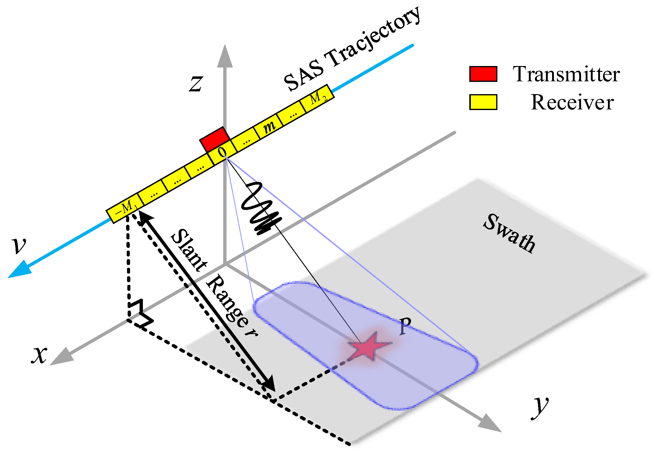
2. The Multi-Receiver SAS’s Model
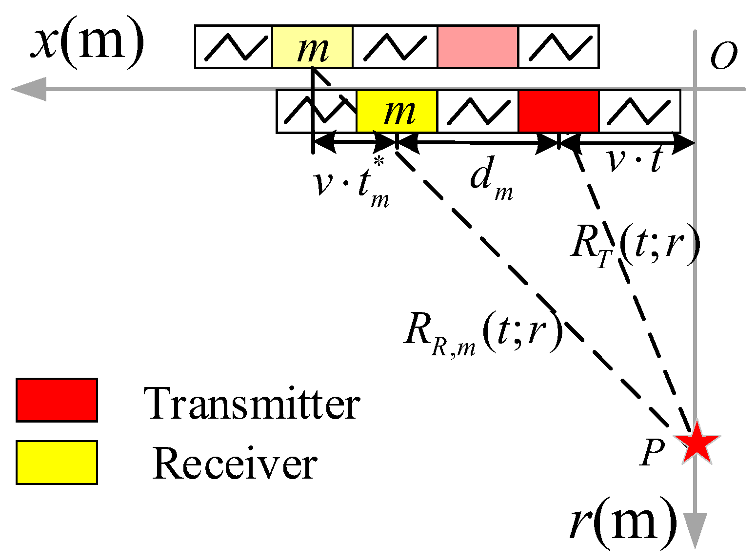
2.1. The Accurate Range History
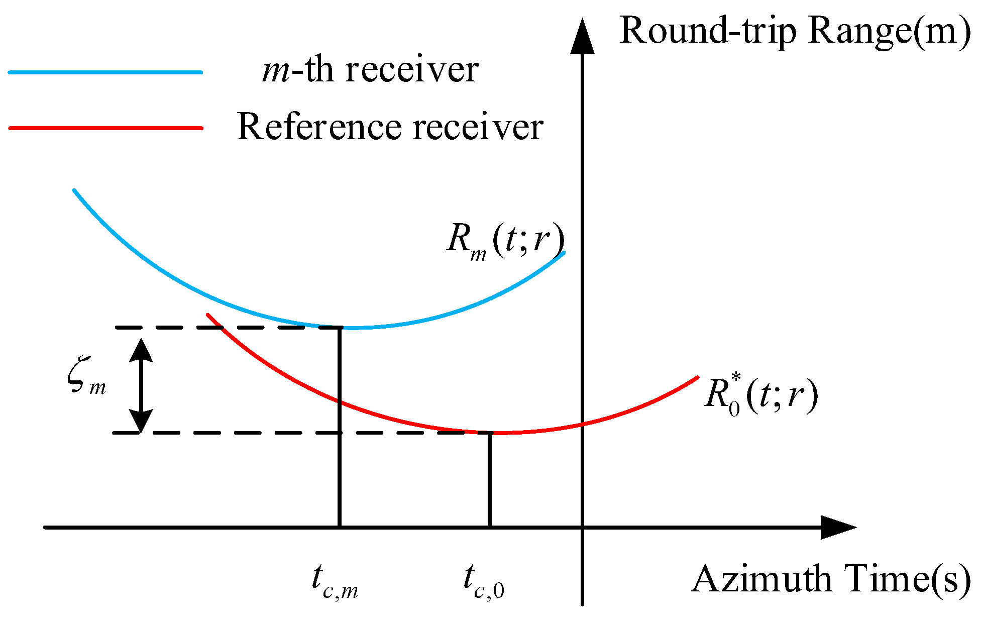
2.2. The Range History Shifting Method
2.3. Derivation of the PTRS
3. The Subblock–Subband CZT Algorithm
3.1. Monostatic Conversion
3.2. Range Time Domain Subblocks
3.3. Range Frequency Domain Subbands
3.4. The CZT Algorithm
4. Simulation and Experimental Results
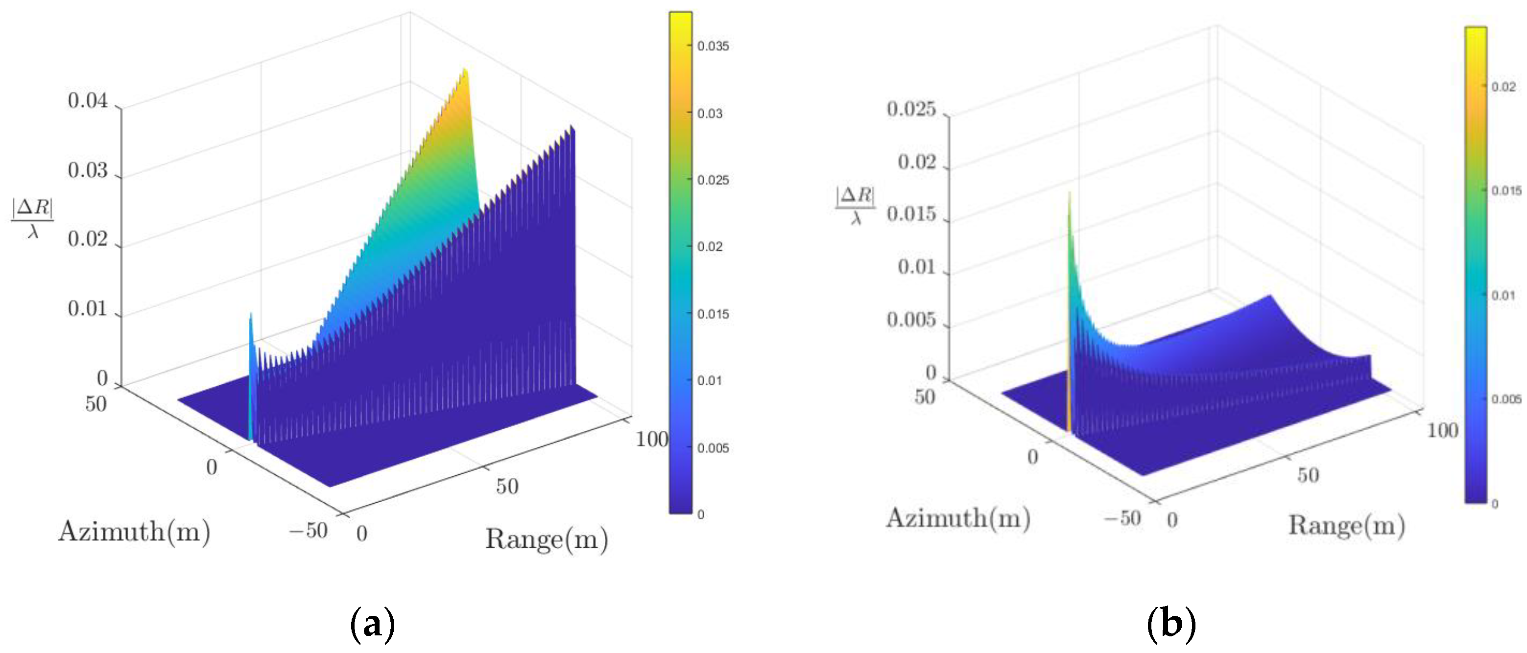
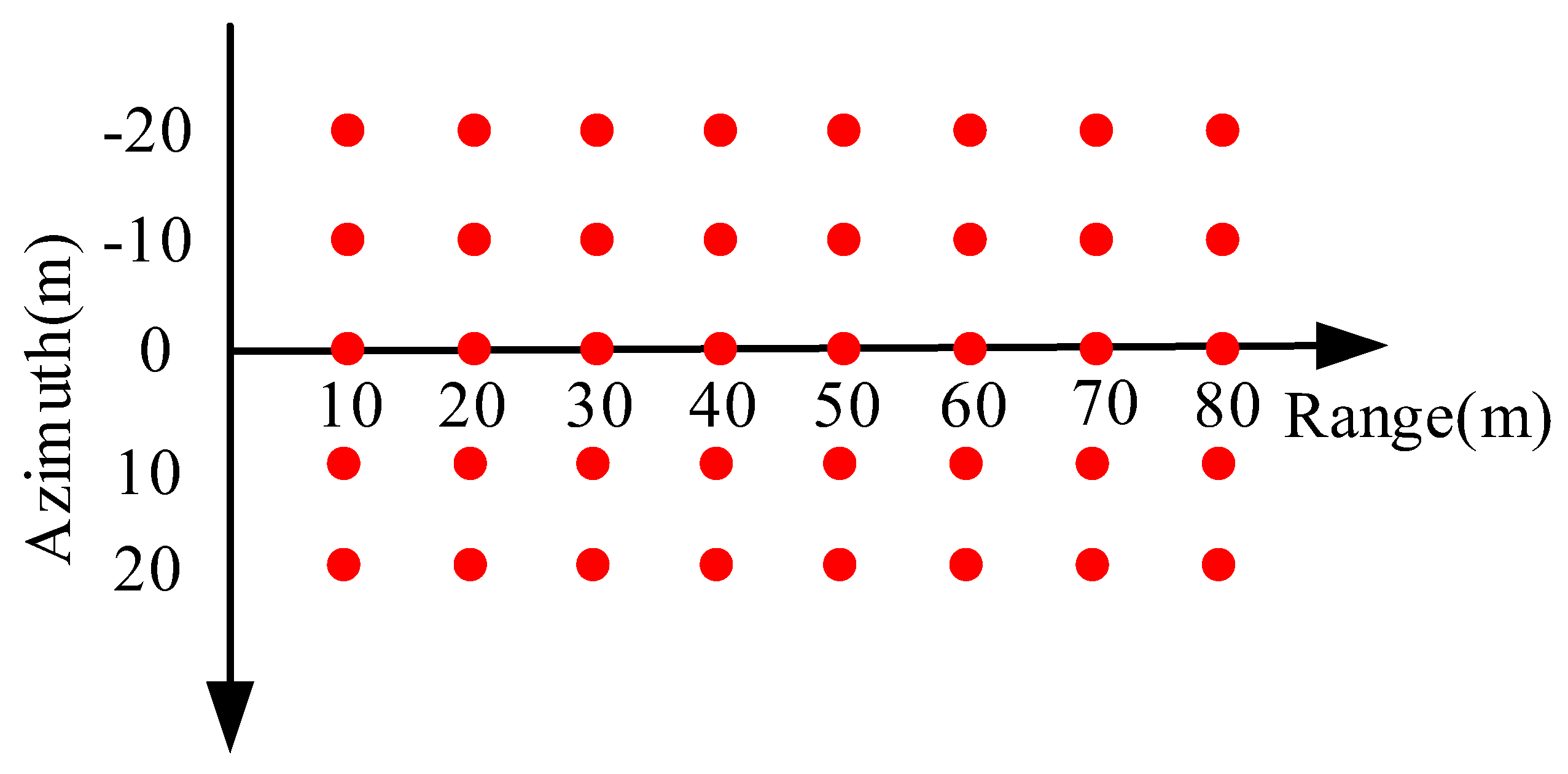
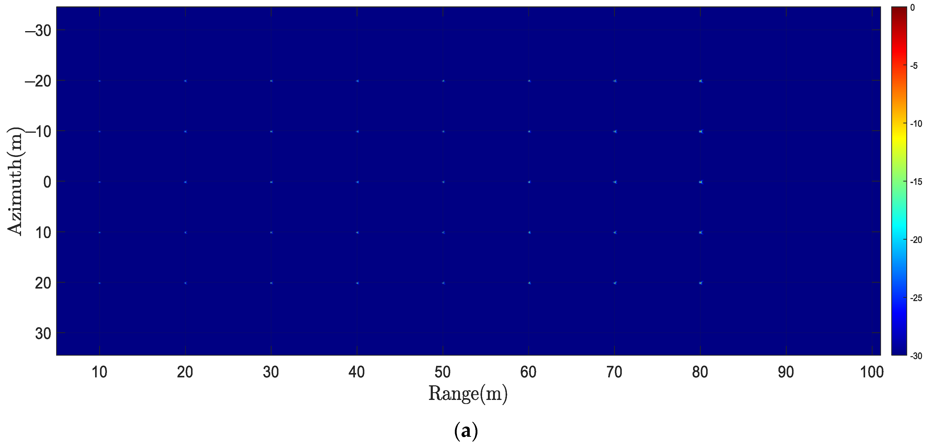
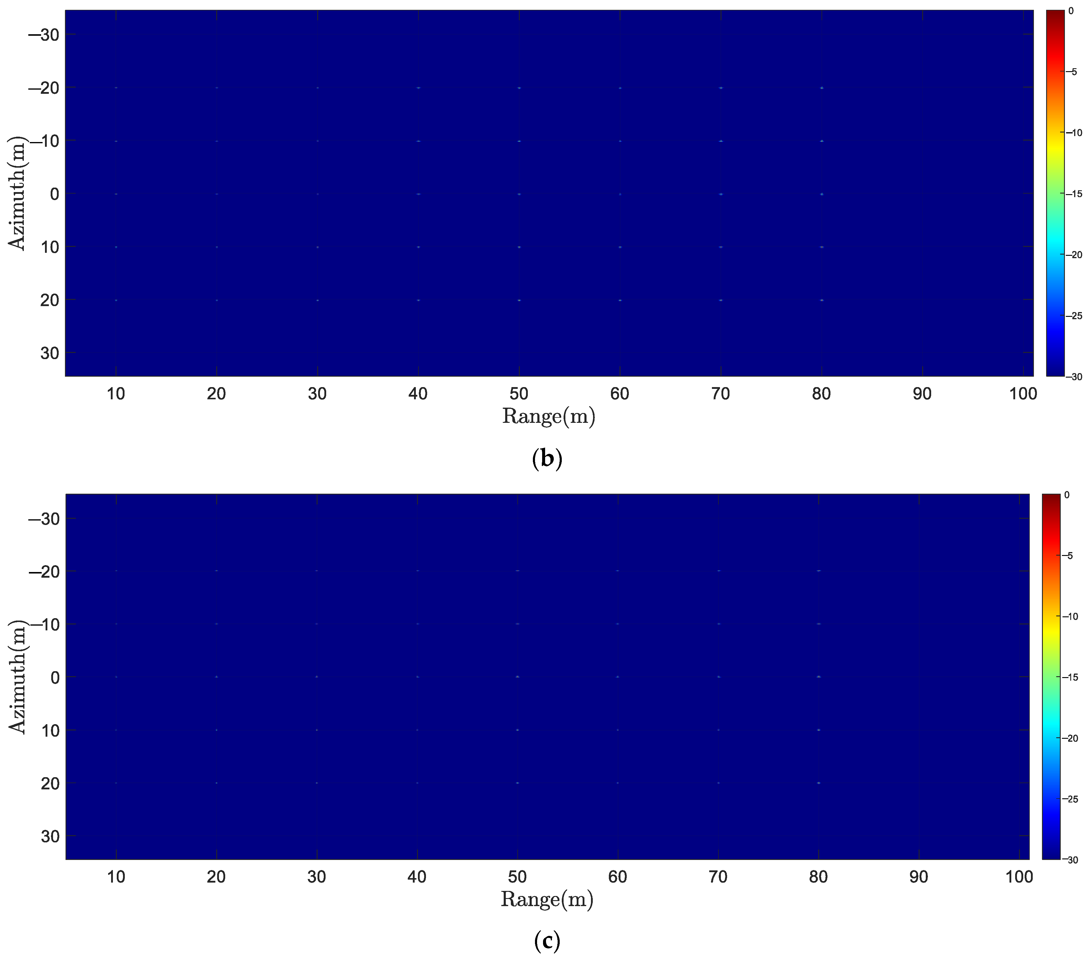
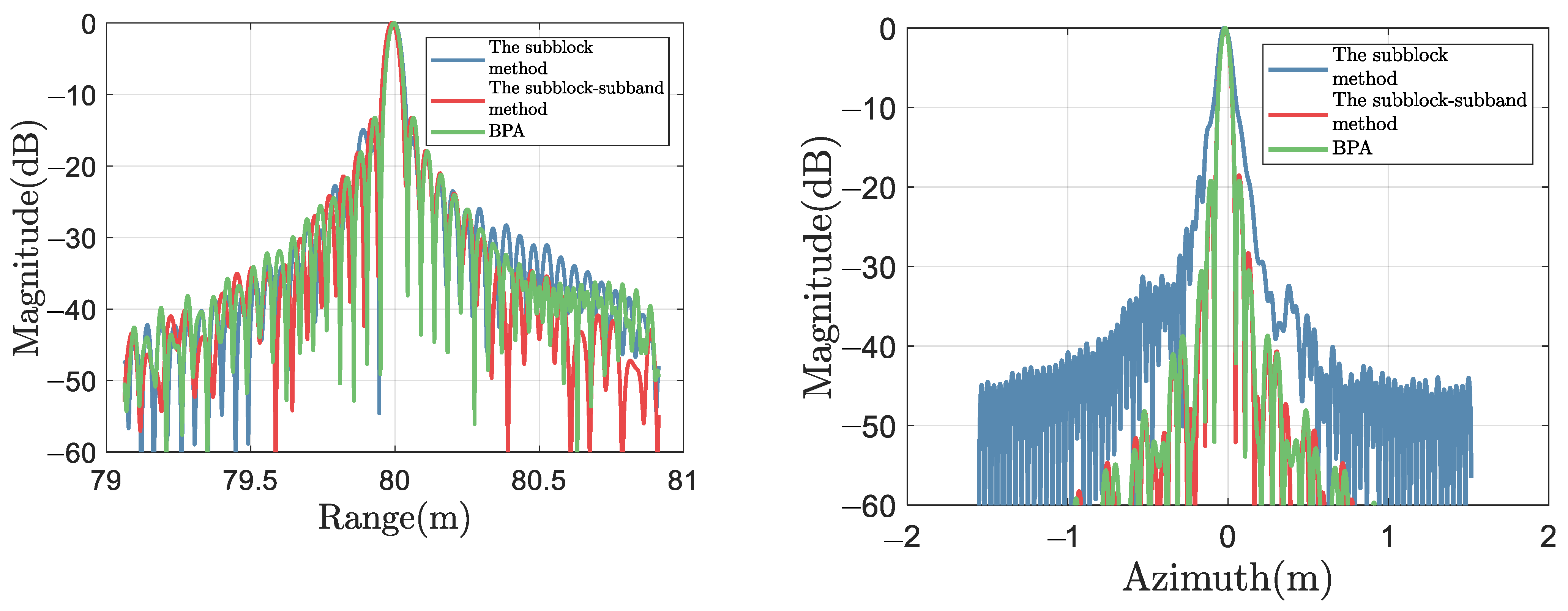
4.1. Computer Simulation
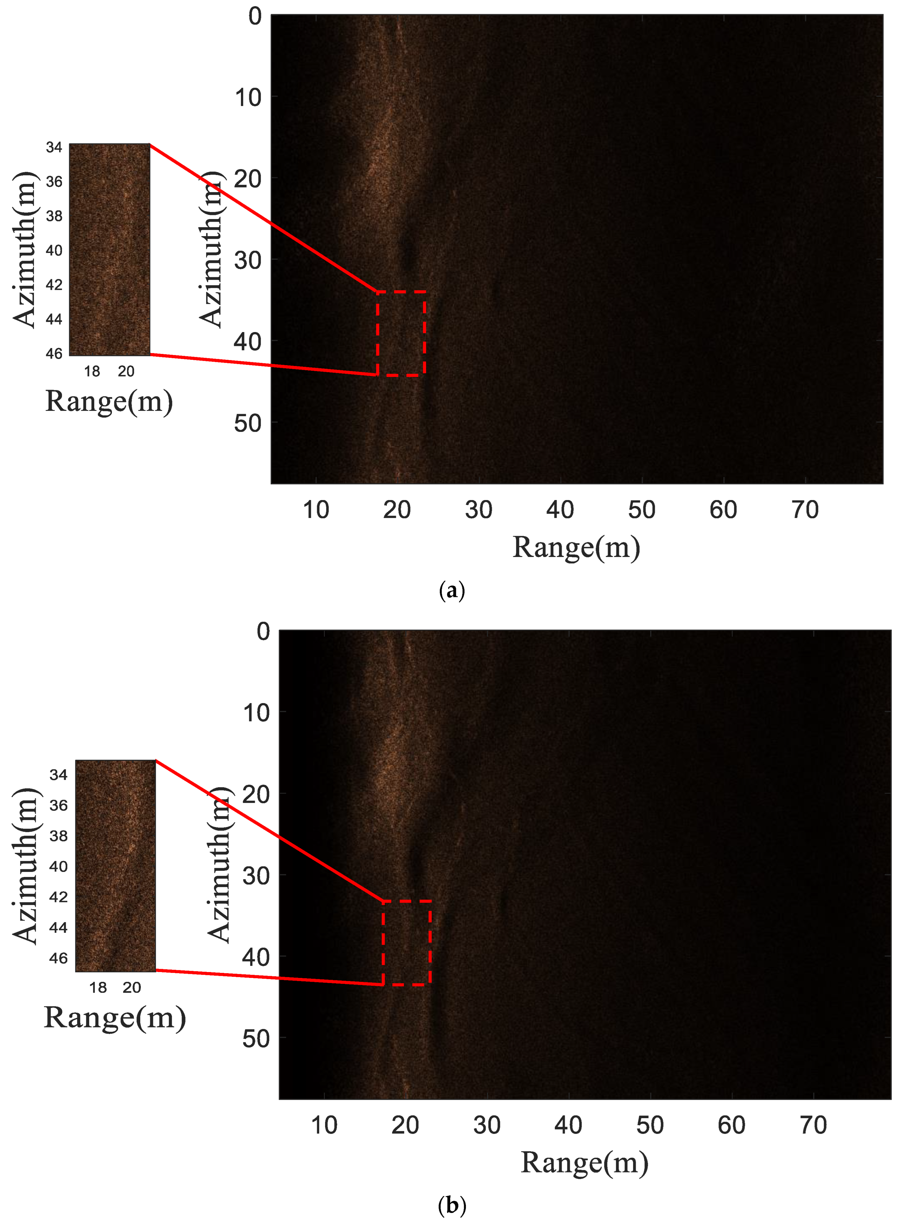
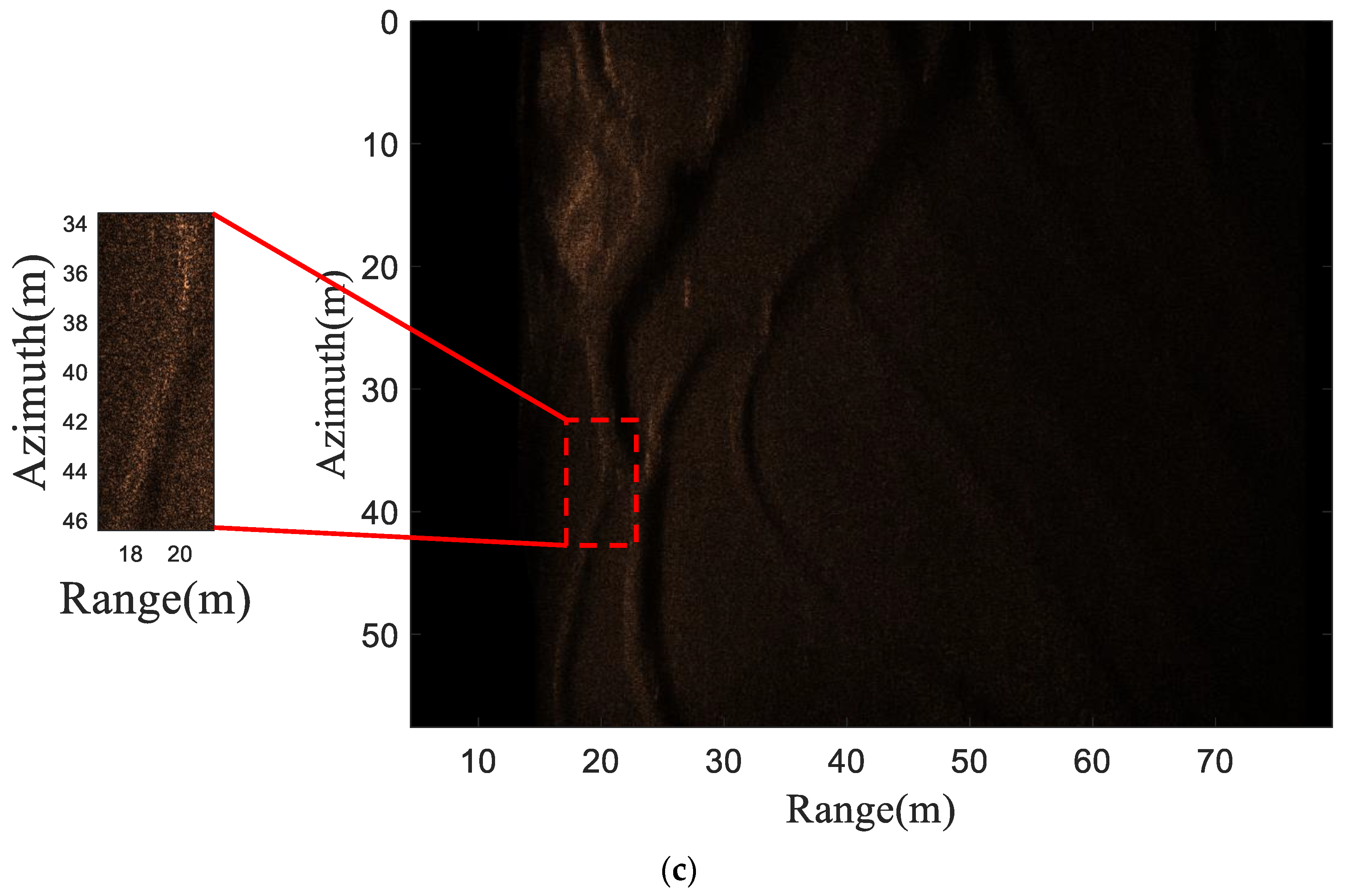
4.2. Real Data Processing
5. Conclusions
Author Contributions
Funding
Data Availability Statement
Acknowledgments
Conflicts of Interest
References
- Putney, A.; Chang, E.; Chatham, R.; Marx, D.; Nelson, M.; Warman, L.K. Synthetic aperture sonar-the modern method of underwater remote sensing. In Proceedings of the IEEE Aerospace Conference Proceedings, Big Sky, MT, USA, 10–17 March 2001. [Google Scholar]
- Marx, D.; Nelson, M.; Chang, E.; Gillespie, W.; Putney, A.; Warman, K. An introduction to synthetic aperture sonar. In Proceedings of the Proceedings of the Tenth IEEE Workshop on Statistical Signal and Array Processing, Manor, PA, USA, 14–16 August 2000. [Google Scholar]
- Xu, J.; Tang, J.-S.; Zhang, C.-H. Multi-aperture Synthetic Aperture Sonar lmaging Algorithm. Signal Process. 2003, 19, 157–160. [Google Scholar] [CrossRef]
- Bruce, M.P. A processing requirement and resolution capability comparison of side-scan and synthetic-aperture sonars. IEEE J. Ocean. Eng. 1992, 17, 106–117. [Google Scholar] [CrossRef]
- Huang, P.; Yang, P.-X. Synthetic aperture imagery for high-resolution imaging sonar. Front. Mar. Sci. 2022, 9, 1049761. [Google Scholar] [CrossRef]
- Zhang, J.-F.; Cheng, G.-L.; Tang, J.-S.; Xie, Z.-M.; Wu, H.-R. A Novel Imaging Algorithm for Wide-Beam Multiple-Receiver Synthetic Aperture Sonar Systems. Remote Sens. 2023, 15, 3745. [Google Scholar] [CrossRef]
- Zhang, X.-B.; Yang, P.-X.; Wang, Y.-M.; Shen, W.-Y.; Yang, J.-C.; Wang, J.-F.; Ye, K.; Zhou, M.-Z.; Sun, H.-X. A Novel Multireceiver SAS RD Processor. IEEE Trans. Geosci. Remote Sens. 2024, 62, 4203611. [Google Scholar] [CrossRef]
- Wu, H.-R.; Zhou, F.-Y.; Xie, Z.-M.; Tang, J.-S.; Zhong, H.-P.; Zhang, J.-F. Two-Dimensional Space-Variant Motion Compensation Algorithm for Multi-Hydrophone Synthetic Aperture Sonar Based on Sub-Beam Compensation. Remote Sens. 2024, 16, 2144. [Google Scholar] [CrossRef]
- Zhang, X.-B. An efficient method for the simulation of multireceiver SAS raw signal. Multimed. Tools Appl. 2024, 83, 37351–37368. [Google Scholar] [CrossRef]
- Sternlicht, D.D.; Femandez, J.E.; Holtzapple, R.; Kucik, D.P.; Montgomery, T.C.; Loeffler, C.M. Advanced sonar technologies for autonomous mine countermeasures. In Proceedings of the OCEANS’11 MTS/IEEE KONA, Waikoloa, HI, USA, 19–22 September 2011. [Google Scholar]
- Fossum, T.G.; Sæbø, T.O.; Langli, B.; Callow, H.; Hansen, R.E. HISAS 1030—High resolution interferometric synthetic aperture sonar. In Proceedings of the Canadian Hydrographic Conference and National Surveyors Conference, Victoria, BC, Canada, 6–7 May 2008. [Google Scholar]
- Zhang, P.; Tang, J.-S.; Zhong, H.-P.; Ning, M.-Q.; Liu, D.-D.; Wu, K. Self-Trained Target Detection of Radar and Sonar Images Using Automatic Deep Learning. IEEE Trans. Geosci. Remote Sens. 2022, 60, 4701914. [Google Scholar] [CrossRef]
- Hagen, P.E.; Hansen, R.; Fossum, T.; Langli, B. Development of High-Resolution Synthetic Aperture Sonar for Demanding AUV Applications. In Proceedings of the 9th Unmanned Underwater Vehicle Showcase, Southampton, UK, 26–27 September 2007. [Google Scholar]
- Zhang, X.; Dai, X.; Yang, B. Fast imaging algorithm for the multiple receiver synthetic aperture sonars. IET Radar Sonar Navig. 2018, 12, 1276–1284. [Google Scholar] [CrossRef]
- Piper, J.E.; Commander, K.W.; Thorsos, E.I.; Williams, K.L. Detection of buried targets using a synthetic aperture sonar. IEEE J. Ocean. Eng. 2002, 27, 495–504. [Google Scholar] [CrossRef]
- Larsen, L.J.; Wilby, A.; Stewart, C. Deep ocean survey and search using synthetic aperture sonar. In Proceedings of the OCEANS 2010 MTS/IEEE SEATTLE, Washington, DC, USA, 20–23 September 2010. [Google Scholar]
- Chatillon, J.; Adams, A.E.; Lawlor, M.A.; Zakharia, M.E. SAMI: A low-frequency prototype for mapping and imaging of the seabed by means of synthetic aperture. IEEE J. Ocean. Eng. 1999, 24, 4–15. [Google Scholar] [CrossRef]
- Neto, A.A.; Rodrigues, G.P.; Alvarenga, I.D. Seabed Mapping with HISAS Sonar For Decommissioning Projects High-Resolution Surveying for Decom Planning. Available online: https://api.semanticscholar.org/CorpusID:49237309 (accessed on 25 June 2024).
- Charlot, D.; Couade, M.; Marty, B.; Fabre, M.N.; Alain, P.; Delbecke, J.; Laquet, T.; Chemisky, B.; Mosca, F.; Bouhier, M.E.; et al. The Synthetic Aperture Mapping Sonar SAMS150 onboard UlyX AUV 6000m: An advanced solution for simultaneous detection and identification of deep-sea features. In Proceedings of the OCEANS 2023, Limerick, Ireland, 5–8 June 2023. [Google Scholar]
- Zhang, X.-B.; Yang, P.-X.; Sun, M. Experiment results of a novel sub-bottom profiler using synthetic aperture technique. Curr. Sci. 2022, 122, 461–464. [Google Scholar] [CrossRef]
- Li, Z.-L.; Yu, Y.-X. Overview of deep water acoustics. Chin. Sci. Bull. 2022, 67, 125–134. [Google Scholar] [CrossRef]
- Dai, W. Research on the Characteristics of Underwater Acoustic Channels and the Propagation Characteristics of Signals in Them. Ship Electron. Eng. 2023, 43, 200–204. [Google Scholar] [CrossRef]
- Shannon, C.E. Communication in the Presence of Noise. Proc. Proc. IRE 1949, 37, 10–21. [Google Scholar] [CrossRef]
- Moreira, A.; Prats-Iraola, P.; Nannini, M.; Martín-del-Campo-Becerra, G.D.; Pardini, M.; Papathanassiou, K.; Reigber, A. Spaceborne Multi-Baseline Synthetic Aperture Radar (SAR) Imaging. In Proceedings of the IEEE International Geoscience and Remote Sensing Symposium, Pasadena, CA, USA, 16–21 July 2023. [Google Scholar]
- Zhang, X.-B.; Tan, C.; Ying, W.-W. Imaging Algorithm for Multireceiver Synthetic Aperture Sonar. J. Electr. Eng. Technol. 2019, 14, 471–478. [Google Scholar] [CrossRef]
- Zhang, X.-B.; Chen, X.-H.; Wu, Q. Influence of the stop-and-hop assumption on synthetic aperture sonar imagery. In Proceedings of the 2017 IEEE 17th International Conference on Communication Technology (ICCT), Chengdu, China, 27–30 October 2017. [Google Scholar]
- Liang, Z.; Fu, X.; Lv, X. New Channel Errors Estimation Method for Multichannel SAR Based on Virtual Calibration Source. Remote Sens. 2021, 13, 3625. [Google Scholar] [CrossRef]
- Lv, Y.-N.; Shang, M.-Y.; Zhong, L.-H.; Qiu, X.-L.; Ding, C.-B. A Novel Imaging Scheme of Squint Multichannel SAR: First Result of GF-3 Satellite. Remote Sens. 2022, 14, 3962. [Google Scholar] [CrossRef]
- Yang, H.-L.; Zhang, S.; Tang, J.-S. Study on Simulation of Multiple-receiver Synthetic Aperture Sonar Imagery Based on Wide Swath. J. Syst. Simul. 2011, 23, 1424–1428. [Google Scholar] [CrossRef]
- Zhang, X.-B.; Liu, Y.-Q.; Deng, X.-Y. Influence of Phase Centre Approximation Error on SAS Imagery. In Proceedings of the 2021 IEEE 6th International Conference on Computer and Communication Systems (ICCCS), Chengdu, China, 23–26 April 2021. [Google Scholar]
- Zhang, X.-B.; Tang, J.-S.; Zhang, S.; Bai, S.-X.; Zhong, H.-P. Four-order Polynomial Based Range-Doppler Algorithm for Multi-receiver Synhetic Aperture Sonar. J. Electron. Inf. Technol. 2014, 36, 1592–1598. [Google Scholar] [CrossRef]
- Neo, Y.L.; Wong, F.; Cumming, I.G. A Two-Dimensional Spectrum for Bistatic SAR Processing Using Series Reversion. IEEE Geosci. Remote Sens. Lett. 2007, 4, 93–96. [Google Scholar] [CrossRef]
- Wu, H.-R.; Jin-Song, T.; Zhong, H.-P.; Yi-Shuo, T. Multi-aperture range-Doppler imaging algorithm based on spectrumofseries reversion. J. Huazhong Univ. Sci. Technol. (Nat. Sci. Ed.) 2018, 46, 6. [Google Scholar] [CrossRef]
- Zhang, X.-B.; Ying, W.-W.; Liu, Y.-Q.; Deng, X.-Y. Processing Multireceiver SAS Data Based on the PTRS Linearization. In Proceedings of the 2021 IEEE International Geoscience and Remote Sensing Symposium IGARSS, Brussels, Belgium, 11–16 July 2021. [Google Scholar]
- Zhang, X.-B.; Yang, P.-X.; Sun, H.-X. Frequency-domain multireceiver synthetic aperture sonar imagery with Chebyshev polynomials. Electron. Lett. 2022, 58, 995–998. [Google Scholar] [CrossRef]
- Zhang, X.-B.; Yang, P.-X.; Dai, X.-T. Focusing Multireceiver SAS Data Based on the Fourth-Order Legendre Expansion. Circuits Syst. Signal Process. 2019, 38, 2607–2629. [Google Scholar] [CrossRef]
- Wang, R.; Loffeld, O.; Ul-Ann, Q.; Nies, H.; Ortiz, A.M.; Samarah, A. A Bistatic Point Target Reference Spectrum for General Bistatic SAR Processing. IEEE Geosci. Remote Sens. Lett. 2008, 5, 517–521. [Google Scholar] [CrossRef]
- Zhang, X.-B.; Wu, H.-R.; Sun, H.-X.; Ying, W.-W. Multireceiver SAS Imagery Based on Monostatic Conversion. IEEE J. Sel. Top. Appl. Earth Obs. Remote Sens. 2021, 14, 10835–10853. [Google Scholar] [CrossRef]
- Wu, J.-J.; Li, Z.-Y.; Huang, Y.-L.; Yang, J.-Y.; Liu, Q.-H. An Omega-K Algorithm for Translational Invariant Bistatic SAR Based on Generalized Loffeld’s Bistatic Formula. IEEE Trans. Geosci. Remote Sens. 2014, 52, 6699–6714. [Google Scholar]
- Zhang, X.-B.; Yang, P.-X.; Wang, Y.-M.; Shen, W.-Y.; Yang, J.-C.; Ye, K.; Zhou, M.-Z.; Sun, H.-X. LBF-Based CS Algorithm for Multireceiver SAS. IEEE Geosci. Remote Sens. Lett. 2024, 21, 1502505. [Google Scholar] [CrossRef]
- Cumming, I.G.; Wong, F.H. Digital Processing of Synthetic ApertureRadar Data: Algorithms and Implementation; Artech House Inc.: Norwood, OH, USA, 2004. [Google Scholar]
- Zhang, X.-B.; Yang, P.-X.; Sun, H.-X. An omega-k algorithm for multireceiver synthetic aperture sonar. Electron. Lett. 2023, 13, e12859. [Google Scholar] [CrossRef]
- Tan, C.; Zhang, X.-B.; Yang, P.-X.; Sun, M. A Novel Sub-Bottom Profiler and Signal Processor. Sensors 2019, 19, 5052. [Google Scholar] [CrossRef]
- Zhang, X.-B.; Wang, Y.-M.; Yang, J.-C.; Shen, W.-Y.; Sun, H.-X. Range-Doppler Imaging Algorithm for Multireceiver Synthetic Aperture Sonar. J. Electron. Inf. Technol. 2022, 44, 2104–2110. [Google Scholar] [CrossRef]
- Zhu, J.-H.; Xie, Z.; Jiang, N.; Song, Y.-P.; Han, S.-D.; Liu, W.-J.; Huang, X.-T. Delay-Doppler Map Shaping through Oversampled Complementary Sets for High-Speed Target Detection. Remote Sens. 2024, 16, 2898. [Google Scholar] [CrossRef]
- Runge, H.; Bamler, R. A Novel High Precision SAR Focussing Algorithm Based On Chirp Scaling. In Proceedings of the 12th Annual International Geoscience and Remote Sensing Symposium, Houston, TX, USA, 26–29 May 1992. [Google Scholar]
- Raney, R.K.; Runge, H.; Bamler, R.; Cumming, I.G.; Wong, F.H. Precision SAR processing using chirp scaling. IEEE Trans. Geosci. Remote Sens. 1994, 32, 786–799. [Google Scholar] [CrossRef]
- Ma, M.-B.; Tang, J.-S.; Zhong, H.-P.; Wu, H.-R. Multireceiver Synthetic Aperture Sonar Chirp Scaling Algorithm Considering Intrapulse Doppler Shift. IEEE J. Ocean. Eng. 2022, 47, 433–444. [Google Scholar] [CrossRef]
- Yang, P.-X. An imaging algorithm for high-resolution imaging sonar system. Multimed. Tools Appl. 2024, 83, 31957–31973. [Google Scholar] [CrossRef]
- Davidson, G.W.; Cumming, I.G.; Ito, M.R. A chirp scaling approach for processing squint mode SAR data. IEEE Trans. Aerosp. Electron. Syst. 1996, 32, 121–133. [Google Scholar] [CrossRef]
- Zhang, X.-B.; Yang, P.-X.; Feng, X.; Sun, H.-X. Efficient imaging method for multireceiver SAS. IET Radar Sonar Navig. 2022, 16, 1470–1483. [Google Scholar] [CrossRef]
- Li, C.; Zhang, H.; Deng, Y.-K. Focus Improvement of Airborne High-Squint Bistatic SAR Data Using Modified Azimuth NLCS Algorithm Based on Lagrange Inversion Theorem. Remote Sens. 2021, 13, 1916. [Google Scholar] [CrossRef]
- Loffeld, O.; Hein, A.; Schneider, F. SAR focusing: Scaled inverse Fourier transformation and chirp scaling. In Proceedings of the IEEE International Geoscience and Remote Sensing Symposium, Seattle, WA, USA, 6–10 July 1998. [Google Scholar]
- Wei, W.; Zhu, D.-Y.; Wu, D. Wavenumber Domain Algorithm Based on the Principle of Chirp Scaling for SAR Imaging. J. Radars 2020, 9, 9. [Google Scholar] [CrossRef]
- Wu, Y.-J.; Huang, Y. Inverse Scaled Fourier Transformation Algorithmfor Squint Mode SAR lmaging. Signal Process. 2010, 26, 4. [Google Scholar]
- Ma, M.-B.; Tang, J.-S.; Wu, H.-R.; Zhang, P.; Ning, M.-Q. CZT Algorithm for the Doppler Scale Signal Model of Multireceiver SAS Based on Shear Theorem. IEEE Trans. Geosci. Remote Sens. 2023, 61, 5201412. [Google Scholar] [CrossRef]
- Ma, M.-B.; Jin-Song, T.; Zhong, H.-P. CZT Algorithm for Multiple-Receiver Synthetic Aperture Sonar. IEEE Access 2020, 8, 1902–1909. [Google Scholar] [CrossRef]
- Ma, M.-B.; Jin-Song, T.; Zhong, H.-P.; Tian, Z. CZT Algorithm for Multiple-receiver Synthetic Aperture Sonar. J. Huazhong Univ. Sci. Technol. (Nat. Sci. Ed.) 2019, 47, 6. [Google Scholar] [CrossRef]
- Franceschetti, G.; Lanari, R.; Marzouk, E.S. A new two-dimensional squint mode SAR processor. IEEE Trans. Aerosp. Electron. Syst. 1996, 32, 854–863. [Google Scholar] [CrossRef]
- Zhang, X.-B.; Yang, P.-X. An Improved Imaging Algorithm for Multi-Receiver SAS System with Wide-Bandwidth Signal. Remote Sens. 2021, 13, 5008. [Google Scholar] [CrossRef]
- Zhang, S.; Jin-Song, T.; Ming, C.; Sheng-Xiang, B. Development and sea trial of interferometric synthetic aperture sonar. Tech. Acoust. 2012, 31, 167–173. [Google Scholar] [CrossRef]
- Raney, R.K. A New And Fundamental Fourier Transform Pair. In Proceedings of the IGARSS ‘92 International Geoscience and Remote Sensing Symposium, Houston, TX, USA, 26–29 May 1992. [Google Scholar]
- Chen, J.-L. Study on Signal Modeling and Imaging Algorithm for Airborne/Spaceborne SAR with Nonlinear Trajectory. Ph.D. Thesis, Xidian University, Xi’an, China, 2018. [Google Scholar]
- Rabiner, L.R.; Schafer, R.W.; Rader, C.M. The chirp z-transform algorithm and its application. Bell Syst. Tech. J. 1969, 48, 1249–1292. [Google Scholar] [CrossRef]
- Bluestein, L. A linear filtering approach to the computation of discrete Fourier transform. IEEE Trans. Audio Electroacoust. 1970, 18, 451–455. [Google Scholar] [CrossRef]
- Zhang, X.-B.; Tang, J.-S.; Wang, F.; Bai, S.-X.; Liu, D.-D. Accurate back projection imaging algorithm for multi-receiverSAS in engineering application. J. Nav. Univ. Eng. 2014, 26, 5. [Google Scholar] [CrossRef]
- Zhang, X.-B.; Yang, P.-X. Back Projection Algorithm for Multi-Receiver Synthetic Aperture Sonar Based on Two Interpolators. J. Mar. Sci. Eng. 2022, 10, 718. [Google Scholar] [CrossRef]
- Zhu, J.-H.; Song, Y.-p.; Jiang, N.; Xie, Z.; Fan, C.-Y.; Huang, X.-T. Enhanced Doppler Resolution and Sidelobe Suppression Performance for Golay Complementary Waveforms. Remote Sens. 2023, 15, 2452. [Google Scholar] [CrossRef]
- Shi, J.-C.; Yu, S.-X. The Analysis of the Error in Sampling. Pet. Instrum. 1995, 9, 154–159. [Google Scholar]


| Parameters | Values |
|---|---|
| Carrier Frequency | 28 kHz |
| Chirp Bandwidth | 16 kHz |
| Pulse duration | 4 ms |
| PRI | 0.15 s |
| Transmitter Size | 0.102 m |
| Receiver Size | 0.0765 m |
| Number of Receivers | 9 |
| SAS Platform Velocity | 2.3 m/s |
| Swath | [5 m, 100 m] |
| Point Targets | Methods | Range Cross-Section | Azimuth Cross-Section | ||||
|---|---|---|---|---|---|---|---|
| PSLR (dB) | ISLR (dB) | IRW (cm) | PSLR (dB) | ISLR (dB) | IRW (cm) | ||
| P1 (0 m, 20 m) | The subblock CZT method | −13.14 | −10.71 | 4.80 | −14.44 | −13.10 | 5.50 |
| The subblock–subband CZT method | −13.17 | −10.42 | 4.76 | −17.42 | −18.94 | 5.74 | |
| BPA | −13.27 | −10.49 | 4.75 | −19.2 | −18.88 | 5.77 | |
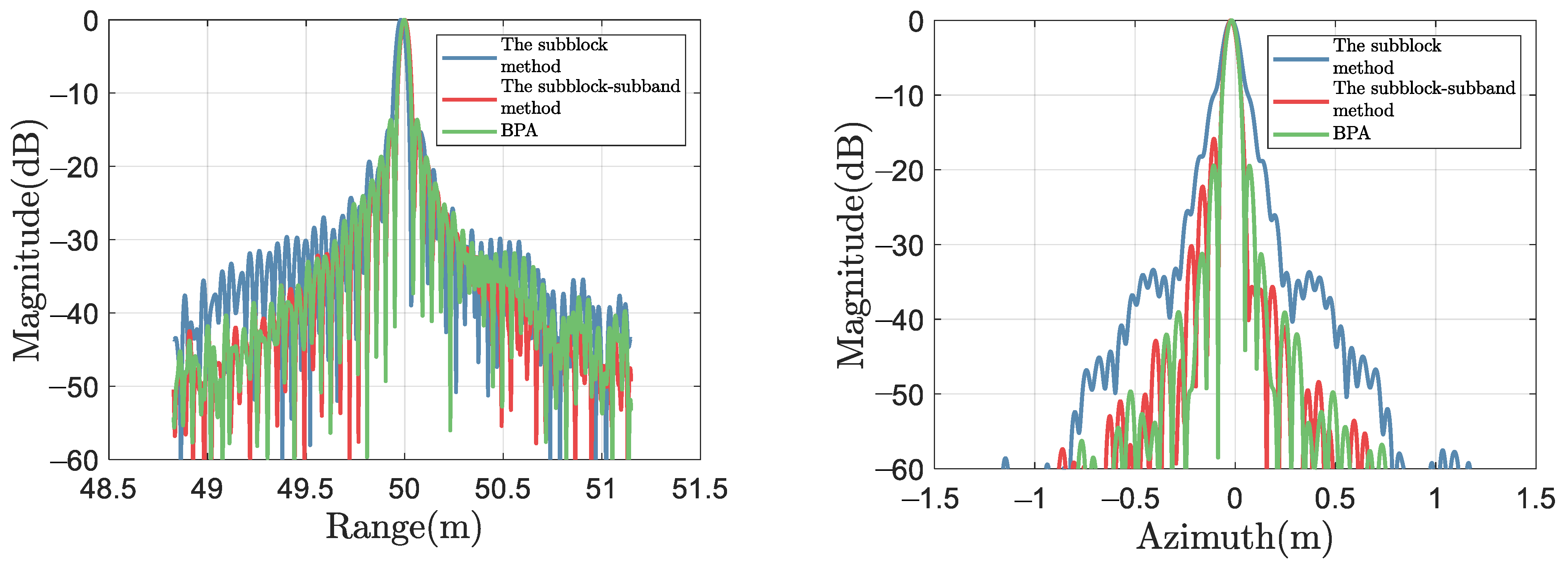
| P2 (0 m, 50 m) | The subblock CZT method | −15.07 | −8.58 | 5.09 | −18.21 | −18.33 | 7.63 |
| The subblock–subband CZT method | −13.17 | −9.7 | 4.89 | −17.87 | −17.91 | 5.61 | |
| BPA | −13.16 | −9.6 | 4.71 | −19.43 | −19.14 | 5.53 | |
| P3 (0 m, 80 m) | The subblock CZT method | −16.06 | −8.62 | 5.03 | −18.53 | −18.03 | 7.41 |
| The subblock–subband CZT method | −13.23 | −9.41 | 4.84 | −18.74 | −19.03 | 5.52 | |
| BPA | −13.23 | −9.43 | 4.78 | −19.21 | −18.87 | 5.54 | |
Disclaimer/Publisher’s Note: The statements, opinions and data contained in all publications are solely those of the individual author(s) and contributor(s) and not of MDPI and/or the editor(s). MDPI and/or the editor(s) disclaim responsibility for any injury to people or property resulting from any ideas, methods, instructions or products referred to in the content. |
© 2024 by the authors. Licensee MDPI, Basel, Switzerland. This article is an open access article distributed under the terms and conditions of the Creative Commons Attribution (CC BY) license (https://creativecommons.org/licenses/by/4.0/).
Share and Cite
Ning, M.; Zhong, H.; Tang, J.; Wu, H.; Zhang, J.; Zhang, P.; Ma, M. A Novel Chirp-Z Transform Algorithm for Multi-Receiver Synthetic Aperture Sonar Based on Range Frequency Division. Remote Sens. 2024, 16, 3265. https://doi.org/10.3390/rs16173265
Ning M, Zhong H, Tang J, Wu H, Zhang J, Zhang P, Ma M. A Novel Chirp-Z Transform Algorithm for Multi-Receiver Synthetic Aperture Sonar Based on Range Frequency Division. Remote Sensing. 2024; 16(17):3265. https://doi.org/10.3390/rs16173265
Chicago/Turabian StyleNing, Mingqiang, Heping Zhong, Jinsong Tang, Haoran Wu, Jiafeng Zhang, Peng Zhang, and Mengbo Ma. 2024. "A Novel Chirp-Z Transform Algorithm for Multi-Receiver Synthetic Aperture Sonar Based on Range Frequency Division" Remote Sensing 16, no. 17: 3265. https://doi.org/10.3390/rs16173265