The Impact of the Expansion and Contraction of China Cities on Carbon Emissions, 2002–2021, Evidence from Integrated Nighttime Light Data and City Attributes

Abstract

Exploring the impact of urbanization on carbon emissions is crucial for formulating effective emission reduction policies. Using nighttime light data and attribute data from 68 Chinese cities (2002–2021), this paper develops an urban development evaluation system with the entropy method. The Lasso method is employed to select key factors affecting carbon emissions, and hierarchical regression models are utilized to analyze these factors across different city types. The results show the following: (1) The extraction of built-up areas using integrated nighttime light data yields an overall accuracy ranging from 70.90% to 98.87%, reflecting high precision. (2) Expanding cities have predominated over the past two decades, indicating a continued upward trend in urbanization in China. (3) Urban development is influenced by internal characteristics and geographic location: contracting cities are mainly inland heavy industrial centers, while expanding cities are located in economically advanced coastal regions. Additionally, it is also impacted by the growth of surrounding cities, exemplified by the imbalance between central cities and their peripheries within metropolitan areas. (4) The expansion of built-up areas is a significant factor affecting carbon emissions across all city types. For expanding cities, managing population growth and promoting tertiary sector development are recommended, while contracting cities should focus on judicious economic planning and virescence area protection.

1. Introduction

Urbanization refers to the process of transitioning rural populations to urban lifestyles. It is characterized by increases in urban population, the expansion of built-up urban areas, the creation of landscapes and urban environments, and changes in social structures and lifestyles [1]. Nearly 4% of the global land has been urbanized, with over 50% of the population living in urban areas [2]. The report from the C40 Cities Climate Leadership Group states that urban areas generate more than four-fifths of global greenhouse gas emissions. The total emissions from urban areas are increasing at an annual rate of 1.8% [3]. With the rapid advancement of urbanization, substantial energy consumption has led to a rise in carbon emissions. Numerous studies have confirmed that the impact of urbanization on carbon emissions is both profound and enduring [4,5].

However, the mechanisms of the impact of urbanization on carbon emissions remain unclear at the theoretical level. Three predominant conclusions have been drawn regarding the relationship between carbon emissions and urbanization: (1) The relationship between carbon emissions and urbanization is positively correlated [6,7,8], and this correlation may be either unidirectional or bidirectional [9,10]. (2) The relationship between carbon emissions and urbanization is negatively correlated [11]. (3) The relationship between carbon emissions and urbanization exhibits an inverted U-shaped curve [12], and this relationship changes with the progress of urbanization [13].

Existing research indicates that the impact of urbanization on carbon emissions exhibits spatial heterogeneity depending on the region. In the United Kingdom and France, there is a clear negative correlation between the urbanization rate and carbon emissions, with increasing urbanization associated with decreasing carbon emissions. In contrast, in Japan and the United States, total carbon emissions initially increase with rising urbanization rates until reaching a turning point, after which they begin to decline as urbanization continues [14,15]. Quantitative studies suggest that in developing countries, a 1% increase in the urbanization rate is associated with approximately a 0.9% increase in carbon emissions [16]. Carbon emissions are observed to peak and decline when the urbanization rate reaches about 75% [17].

The urbanization of China began late, and its urbanization rate remains lower. There is still a significant positive correlation between carbon emissions and urbanization rate [14]. Additionally, China is one of the world’s largest carbon emitters. China has announced a reduction in carbon intensity by over 60% from 2005 levels by 2030. Carbon removals and emissions must be balanced by 2060 [18,19,20,21]. Studying the relationship between urban development and carbon emissions in Chinese cities can offer useful insights for global carbon reduction efforts and support goals for reaching the carbon peak and carbon neutrality. Moreover, with the large number of cities in China and the variety of urbanization types, examining this relationship can help manage differences in urban development and provide a basis for guiding cities towards high-quality, low-carbon, and sustainable growth.

Urbanization is related to population migration, changes in land use, and changes in production methods; therefore, its impact on carbon emissions is multifaceted [22,23]. Existing research suggests that changes in urban population structure and increased population density are direct factors affecting carbon emissions [23,24]. The rise in consumption levels in urban areas, coupled with an increased demand for energy, contributes to an increase in carbon emissions [25,26]. In the latter phases of industrialization, the refinement of industrial structures and technological advancements serve as instrumental factors in managing the escalation of carbon emissions [27,28]. The transformation of the economic structure has enabled the service industry to drive carbon emissions more than other industries [29]. Additionally, the expansion of urban construction land can influence carbon emissions by altering aspects such as urban transportation and green spaces [30,31,32]. In addition, some research indicates that the impact of urbanization on carbon emissions results from the interplay of multiple factors. For instance, economic development can improve education levels, which in turn affects public awareness and perceptions of carbon emissions [33,34]. Therefore, in order to study the relationship between carbon emissions and urbanization, it is necessary to analyze it from multiple perspectives.

Conventional data are subject to long update cycles and other limitations, making it difficult to examine the spatiotemporal characteristics of urbanization over a long time series. Compared with traditional methods, remote sensing technology has timeliness and wide spatial coverage. As a remote sensing data source that captures and records faint light radiation from the Earth’s surface at night in real-time, nighttime light (NTL) data can reflect human activities accurately to some extent [35]. NTL observations have proven to be effective in tracking light sources generated by human activities. This capability aids in assessing the spatiotemporal changes in socio-economic activities and urbanization processes [36,37]. Numerous studies have used NTL data to reveal the external features of cities, such as extracting city boundaries [38] and detecting city centers and their spatial structures [39]. At the same time, NTL data have the advantages of a large scale and long time series, and are widely used to display the spatiotemporal dynamic changes of cities or urban agglomerations [40,41]. Therefore, combining nighttime light data with statistical data can not only obtain indicators of urban socio-economic changes, but also obtain long-term urban morphological structural characteristics, which is conducive to jointly analyzing the key factors affecting carbon emissions from both inside and outside the city.

This study uses multi-temporal built-up area data and nighttime light (NTL) data as sources to propose a method for integrating remote sensing data with statistical data into an urbanization development assessment system. The aim is to investigate the key factors influencing carbon emissions under different urbanization development models and to expand the understanding of the mechanisms through which urbanization impacts carbon emissions. We have three objectives:(1) to integrate two types of nighttime light data to get a long time series data set of the built-up areas of Chinese cities; (2) to establish an urban development evaluation system and classify cities according to their development status; and (3) to exam the similarities and differences in the factors affecting carbon emissions in different types of cities.

2. Materials and Methods

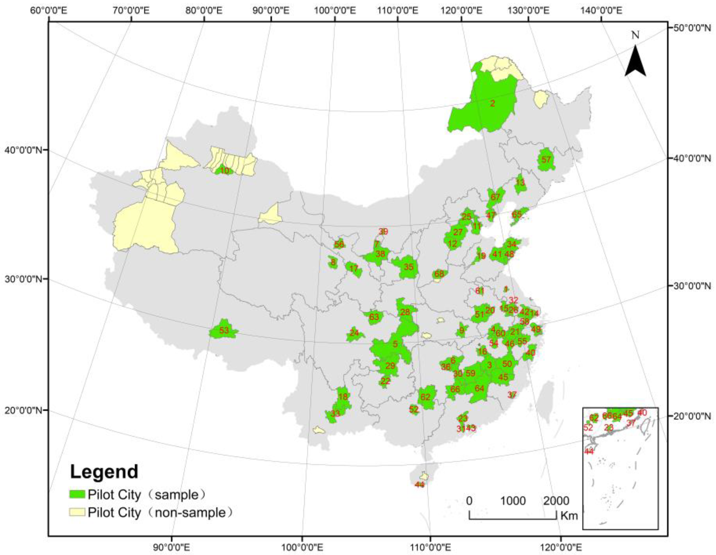
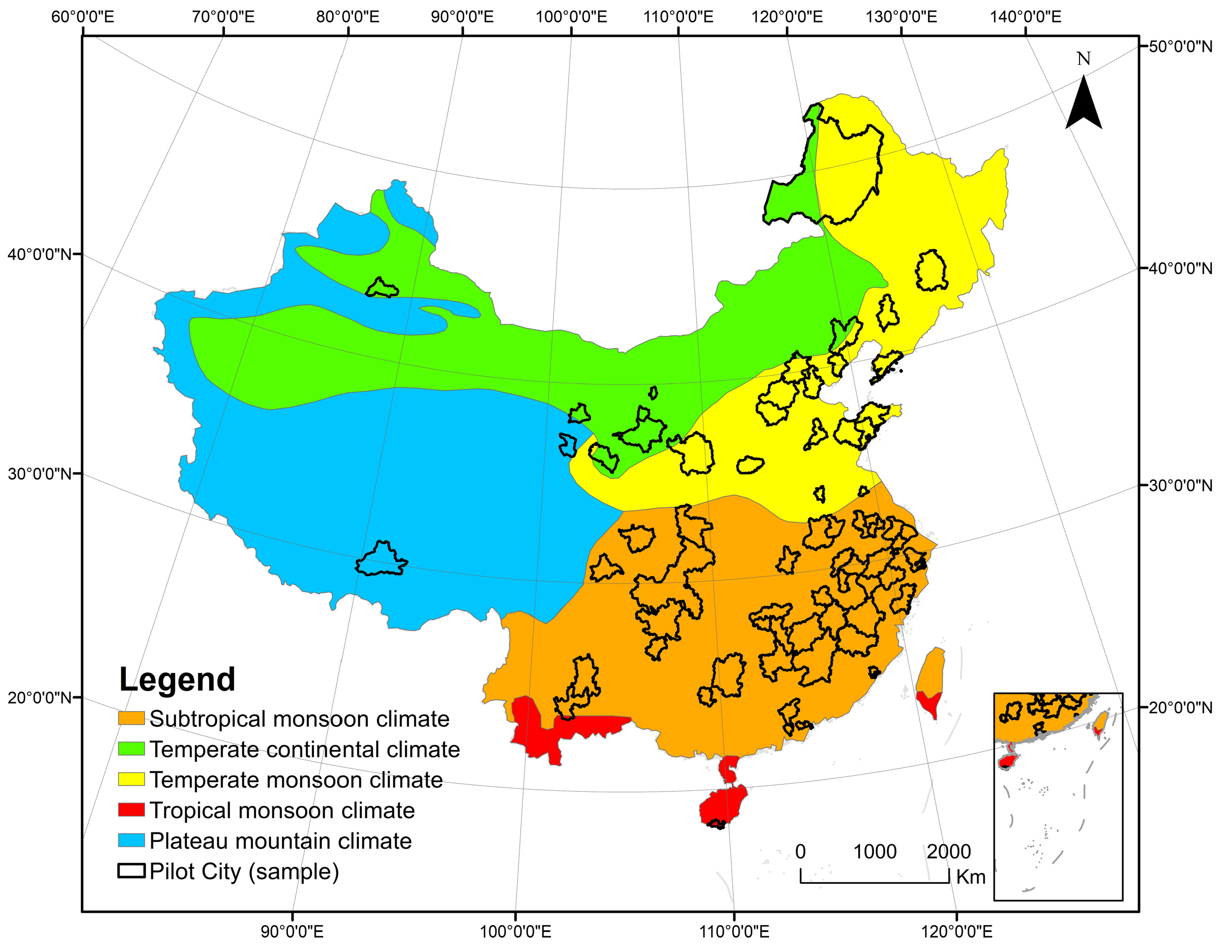
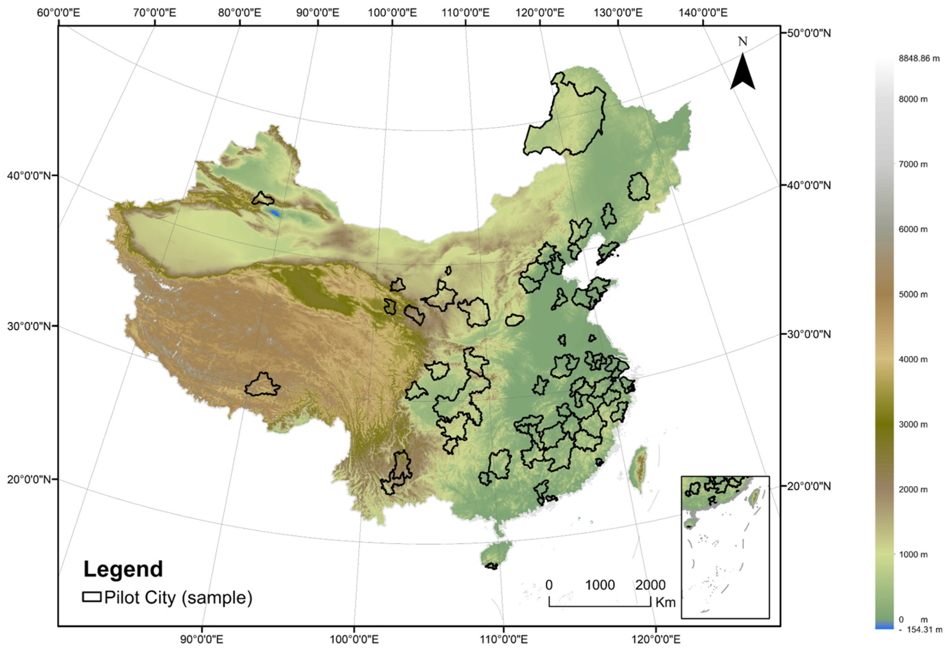
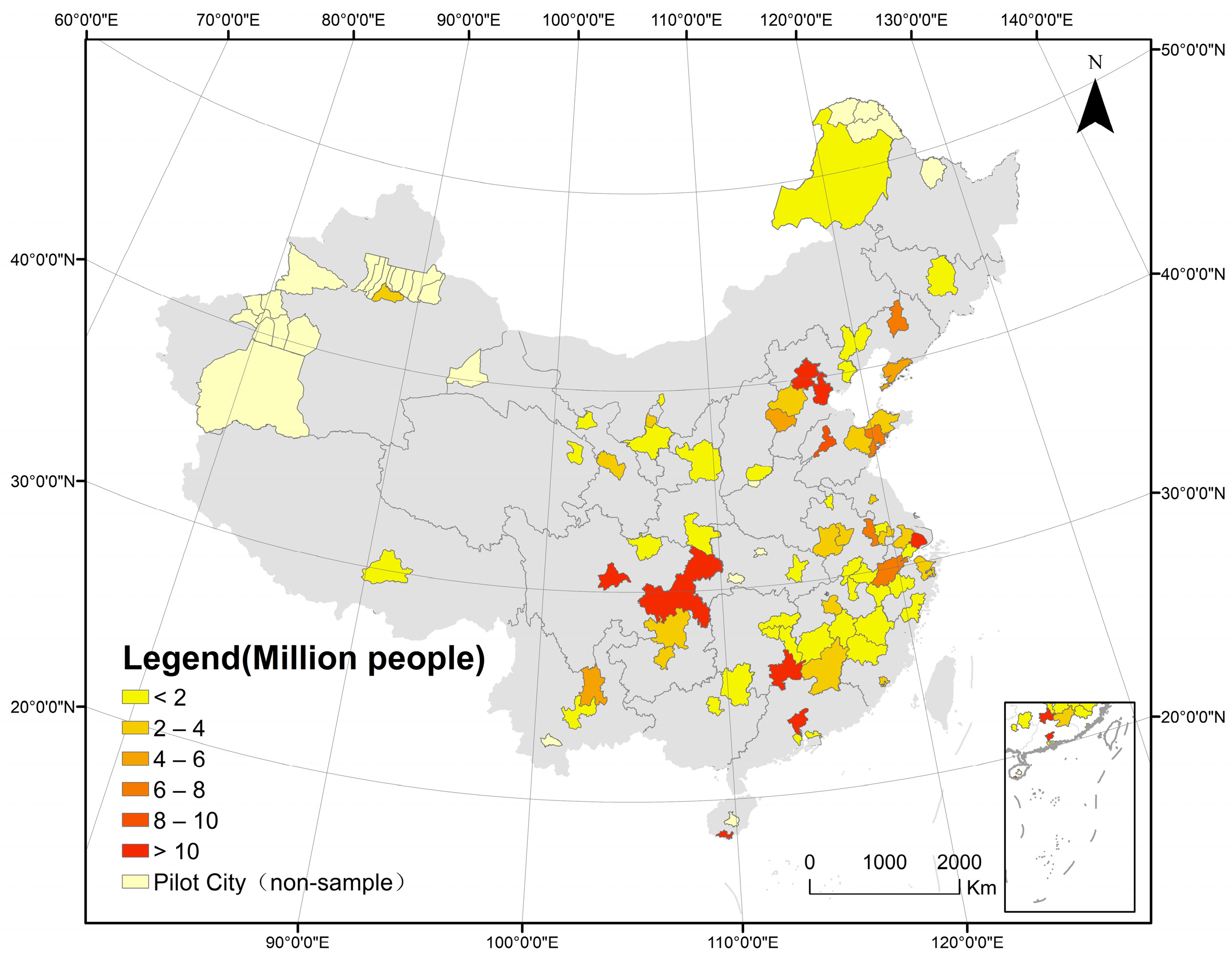
2.1. Study Area

In order to promote sustainable development and fulfill international environmental responsibilities, China established three batches of urban low-carbon pilot projects including 81 cities from 2010 to 2020 to undertake low-carbon initiatives (Figure 1). The data in some cities are incomplete, so this paper selects 68 of them as the focus of research. The city and its corresponding serial number can be found in Appendix A,

Table A1. 68 sample cities selected for this paper.

Number	City	Number	City	Number	City
1	Huai’an	24	Chengdu	47	Qinhuangdao
2	Hulun Buir	25	Beijing	48	Qingdao
3	Fuzhou	26	Changzhou	49	Ningbo
4	Chizhou	27	Baoding	50	Nanping
5	Chongqing	28	Ankang	51	Lu’an
6	Changsha	29	Zunyi	52	Liuzhou
7	Yinchuan	30	Zhuzhou	53	Lhasa
8	Xining	31	Zhongshan	54	Jingdezhen
9	Wuhan	32	Zhenjiang	55	Jinhua
10	Urumqi	33	Yuxi	56	Jinchang
11	Tianjin	34	Yantai	57	Jilin
12	Shijiazhuang	35	Yan’an	58	Jiaxing
13	Shenyang	36	Xiangtan	59	Ji’an
14	Shanghai	37	Xiamen	60	Huangshan
15	Nanjing	38	Wuzhong	61	Huaibei
16	Nanchang	39	Wuhai	62	Guilin
17	Lanzhou	40	Wenzhou	63	Guangyuan
18	Kunming	41	Weifang	64	Ganzhou
19	Jinan	42	Suzhou	65	Dalian
20	Hefei	43	Shenzhen	66	Chenzhou
21	Hangzhou	44	Sanya	67	Chaoyang
22	Guiyang	45	Sanming	68	Jincheng
23	Guangzhou	46	Quzhou

.

From a geographical perspective, these pilot cities span across China, ranging from the Greater Khingan Range in the north to Sanya in Hainan Province in the south. They encompass five distinct climate types: temperate continental climate, temperate monsoon climate, subtropical monsoon climate, tropical monsoon climate, and plateau mountain climate (Figure 2). At the same time, the topography of low-carbon pilot cities is quite varied. In the eastern plain regions, these cities are often grouped together, while in the central and western plateau regions, they are more spread out (Figure 3).

From a social perspective, the 81 pilot cities encompass China’s four major economic zones: the Beijing–Tianjin–Hebei region, the Yangtze River Delta, the Pearl River Delta, and the Chengdu–Chongqing urban agglomeration. The varying functions and development timelines of these city clusters result in differences in their levels of development. Additionally, there are notable disparities in their scales and functions, including traditional industrial cities such as Wuhai and Zhuzhou, as well as economically open regions such as Shenzhen and Xiamen. Figure 4 and Figure 5 reveal significant differences in economic and population scales among the cities. For example, cities like Shanghai and Beijing are densely populated and economically advanced, while cities such as Urumqi and Lhasa are sparsely populated and less economically developed.

The diverse distribution of low-carbon pilot cities facilitates the development of tailored policies, addressing the specific needs of different types of cities. The last batch of pilot cities was initiated late, resulting in limited research focused on these cities as study areas. Using these pilot cities as samples not only meets the requirement for diversity in the study area but also provides valuable insights for developing effective low-carbon policies in China.

2.2. Data Sources

There are two types of widely used nighttime light data. The DMSP/OLS nighttime light data are provided by the National Geophysical Data Center (NGDC) of the National Oceanic and Atmospheric Administration (NOAA). The dataset, available for download, includes 34 images spanning from 1992 to 2013, with a spatial resolution of approximately 1 km and grayscale levels ranging from 0 to 63. DMSP/OLS data from 2002 to 2013 are utilized in this experiment.

The National Polar-orbiting Partnership (NPP) satellite is a new-generation Earth observation system operated by the United States, developed collaboratively by the National Aeronautics and Space Administration (NASA), the National Oceanic and Atmospheric Administration (NOAA), and the U.S. Air Force. The satellite provides monthly data with a spatial resolution of 500 m, available from 2012 onwards. This study utilizes monthly NPP-VIIRS data from 2012 to 2021, which are aggregated into annual datasets.

Specifically, DMSP/OLS data from 2012 and 2013, along with NPP-VIIRS data, are used to integrate the two types of nighttime light data.

The MODIS land cover type product MCD12Q1 is selected for the accuracy evaluation of built-up area extraction. MCD12Q1 is a MODIS land cover type product that provides an annual global distribution of land cover types with a resolution of 500 m. The data are used for the accuracy assessment of built-up area extraction. This paper extracts the built-up areas of the pilot cities from 2002 to 2021. To ensure the validity of the accuracy assessment, MODIS data from 2010 and 2020 are selected for the validation process.

The carbon emission data at the city level used in this study are from the China Emission Accounts and Datasets (CEADs). CEADs have compiled carbon accounting inventories covering China and other developing countries, with the aim of establishing a cross-validated multi-scale carbon emissions accounting methodology, and creating a regionally and locally unified, detailed carbon accounting data platform [42,43,44]. CEADs provide a carbon emission inventory for Chinese cities from 1997 to 2019. Because the data before 2006 are incomplete, data from 2006 to 2019 are used to analyze the factors influencing carbon emissions.

The urban statistical data and energy data are sourced from the China Urban Statistical Yearbook (2002–2021) and the China Energy Statistical Yearbook (2002–2021).

The information of the data used in this paper is shown in

Table 1. Research data and their sources.

Dataset	Data	Source
DMSP/OLS nighttime light data	2002–2013	https://eogdata.mines.edu/products/vnl/ (accessed on 1 September 2023)
NPP-VIIRS nighttime light data	2012–2021
The MODIS land cover type product MCD12Q1	2010, 2020	https://ladsweb.modaps.eosdis.nasa.gov
The China Emission Accounts and Datasets (CEADs)	2006–2019	https://www.ceads.net.cn/
The urban statistical data and energy data	2002–2021	http://www.stats.gov.cn/

.

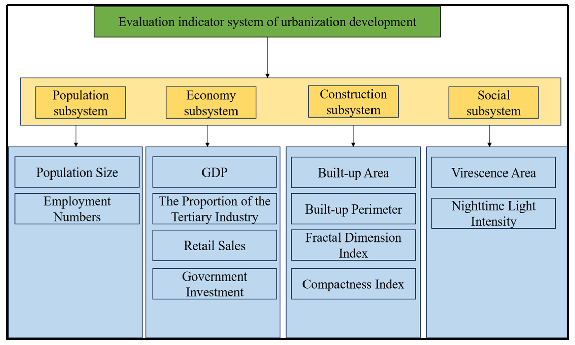
2.3. Urban Development Evaluation System

Different dimensions of urbanization have varying influences on the carbon emissions of urban ecosystems. Currently, most scholars believe that urbanization development can be subdivided into population, economic, social, land, and ecological urbanization [45,46]. Some scholars have also described the complexity of urbanization from the perspectives of population, building structure, and greenness [47]. Based on the existing research, this paper establishes an evaluation system for urbanization development composed of a population subsystem, economic subsystem, construction subsystem, and society subsystem. The primary indicator of the evaluation system is the overall score of urban development. Population, economy, urban construction, and society subsystems constitute the secondary indicators of the evaluation system. Each subsystem contains 2–4 tertiary indicators. Figure 6 shows the composition of the urbanization development evaluation system. The following is an explanation of the selection of indicators.

Two indicators are selected to form a population subsystem: population size (PS) and employment numbers (ENs). GDP, the proportion of the tertiary industry (PTI), retail sales (RSs) and government investment (GI) are chosen to represent the economy subsystem. For the social subsystem, virescence area (VA) represents the environmental evaluation factor and night light intensity (NLI) is selected as the human activity evaluation factor.

The built-up area (BA) and built-up perimeter (BP) regions are obtained after integrating two types of nighttime light data. The Fractal Dimension Index (FDI) and Compactness Index (CI) are also calculated. These four metrics are used to construct a development subsystem. The CI is usually used to reflect the shape characteristics of a region. The FDI can reflect the tortuosity and complexity of the shape.

The formulas for FDI and CI are as follows [48]:

$$FDI=2\ln (P/4)/\ln A$$

(1)

$$CI=2\sqrt{\pi A}/P$$

(2)

$P$ represents the perimeter of the built-up area, and $A$ represents the area of the built-up area.

The multi-index evaluation method is used to establish an urban development evaluation system, which combines various indicators by measuring the impact of each one on the city, thereby forming an evaluation system. Firstly, this paper employs the normalization of evaluation indicators to eliminate the influence of different units and dimensions among various indicators. The standardized data results lie within the range of [0, 1]. To ensure the universality of the evaluation system, this study employs the objective weighting method known as the entropy method to determine the weights of the evaluation indicators. After establishing the evaluation system, a 5-year cycle is adopted to calculate the rate of change in urban scores. Based on this rate of change, cities are classified into three categories: contracting city ($C<-0.1$), stable city $(-0.1<C<0.1)$, and expanding city $(C>0.1)$.

The process of establishing the urbanization development evaluation system is shown in

Table 2. The process of establishing the urbanization development evaluation system.

Method	Step	Formula	Meaning
Min–Max Normalization		$X_{it}=(X-X_{t_{\min }})/(X_{t_{\max }}-X_{t_{\min }})$	$X_{it}$$\mathrm{is} \mathrm{the} \mathrm{standardized} \mathrm{data} \mathrm{for} \mathrm{city} i$$\mathrm{year} t$. $X_{t_{\min }}$$\mathrm{and} X_{t_{\max }}$ is the minimum and maximum values in the data of 68 cities in year t.
Information Entropy Method	$\mathrm{The} \mathrm{proportion} \mathrm{of} \mathrm{city} i$$\mathrm{indicator} j$ to all cities	$y_{ij}=x_{ij}/{\displaystyle \sum _{i,j}^r{x}_{ij}}$	$X_{ij}$$\mathrm{is} \mathrm{the} \mathrm{standardized} \mathrm{data} \mathrm{for} \mathrm{city} i$$\mathrm{indicator} j$. $y_{ij}$$\mathrm{is} \mathrm{the} \mathrm{weight} \mathrm{of} \mathrm{indicator} j$$\mathrm{in} \mathrm{city} i$. $e_{ij}$$\mathrm{is} \mathrm{the} \mathrm{entropy} \mathrm{value} \mathrm{of} \mathrm{indicator} j.$ $r$ is the number of sample cities. $m$$\mathrm{is} \mathrm{the} \mathrm{number} \mathrm{of} \mathrm{indicators}.$ $E_i \mathrm{is} \mathrm{the} \mathrm{score} \mathrm{of} \mathrm{city} i$.
	$\mathrm{Entropy}\mathrm{value}\mathrm{of}\mathrm{indicator}j$	$e_j=-(1/\ln r)\times {\displaystyle \sum _{i=1}^r{y}_{ij}\times \ln y_{ij}}$
	$\mathrm{Information}\mathrm{utility}\mathrm{value}\mathrm{of}\mathrm{the}\mathrm{entropy}\mathrm{value}\mathrm{of}\mathrm{indicator}j$	$d_j=1-e_j$
	$\mathrm{Weight}\mathrm{of}\mathrm{indicator}j$	$w_j=d_j/{\displaystyle \sum _{j=1}^m{d}_j}$
	$\mathrm{Score} \mathrm{for} \mathrm{the} \mathrm{development} \mathrm{of} \mathrm{city} i$	$E_i={\displaystyle \sum _{j=1}^m{w}_j\times x_{ij}}$
Urban development change rate		$C_{it}=(E_{i{t}_1}-E_{i{t}_0})/E_{i{t}_0}$	$C_{it}$$\mathrm{is} \mathrm{the} \mathrm{change} \mathrm{rate} \mathrm{of} \mathrm{period} t$$\mathrm{in} \mathrm{city} i$. $E_{i{t}_0} \mathrm{and} E_{i{t}_1} \mathrm{are} \mathrm{the} \mathrm{scores} \mathrm{of} \mathrm{city} i \mathrm{in} \mathrm{the} \mathrm{early} \mathrm{and} \mathrm{late} \mathrm{stages} \mathrm{of} \mathrm{period} t.$

[49].

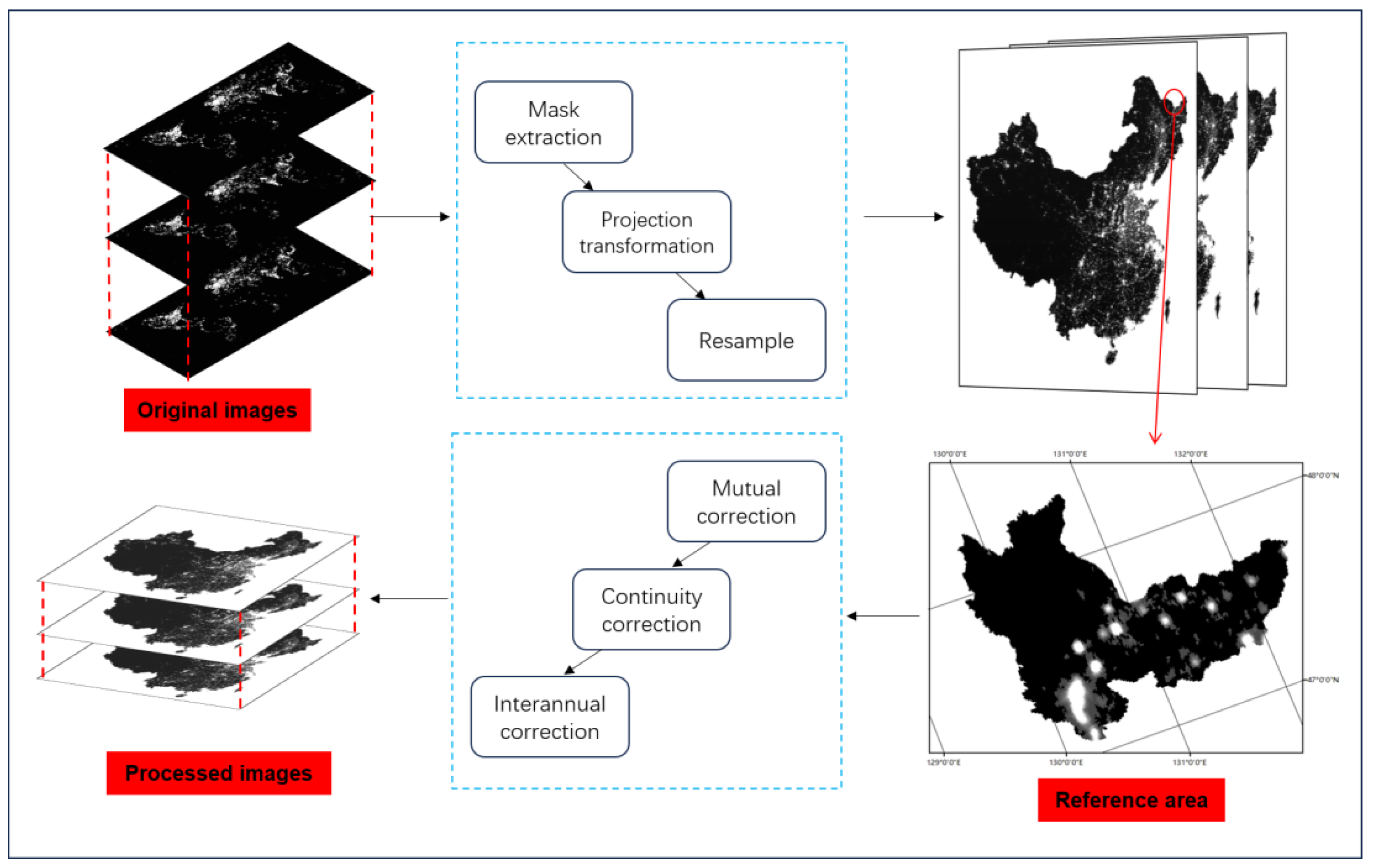
2.4. Using Nighttime Light Images to Extract Built-Up Areas

The radiometric performance and detection capabilities of different sensors on the DMSP satellites vary, leading to certain limitations in the DMSP/OLS data. Therefore, the first step involves preprocessing the DMSP/OLS data, as illustrated in Figure 7. Firstly, the imagery is extracted using Chinese vector data as a boundary. The extracted image is then converted to the Albers projection and resampled to a resolution of 1 km. As the data are sourced from multiple satellites, it is necessary to minimize differences among the data through mutual calibration. Generally, Hegang City in Heilongjiang is used as the reference area, and the F162006 image is used as the reference image. This is used to establish correspondences between the other 33 images and the reference image. The mutually corrected images still have discontinuity problems, so the images need to be further corrected for continuity. In a long time series of DMSP/OLS data, bright pixel values in the image from the previous year may become non-bright values or exhibit different DN values at the same location in the image from the subsequent year. To address this unusual fluctuation, it is necessary to conduct an interannual correction on the pixels after the continuity correction. The preprocessing process of DMSP/OLS data is shown in

Table 3. Calculation for mutual correction, continuity correction, and interannual correction.

Step	Formula	Meaning
Mutual correction	$D{N}_{cal}=a\times D{N}^2+b\times DN+c$	$DN$$\mathrm{is} \mathrm{the} \mathrm{DN} \mathrm{value} \mathrm{of} \mathrm{the} \mathrm{pixel} \mathrm{to} \mathrm{be} \mathrm{corrected}.$ $D{N}_{cal} \mathrm{is} \mathrm{the} \mathrm{DN} \mathrm{value} \mathrm{of} \mathrm{the} \mathrm{pixel} \mathrm{after} \mathrm{correction}.$ a, b, c are the parameters obtained from quadratic regression.
Continuity correction	$D{N}_{(n,i)}=\left\{\begin{array}{l}0\hspace{1em}\hspace{1em}\hspace{1em}\hspace{1em}\hspace{1em}\hspace{1em}\hspace{1em}\hspace{1em}D{N}_{(n,i)}^a=0 and D{N}_{(n,i)}^b=0\hfill \\ (D{N}_{(n,i)}^a+D{N}_{(n,i)}^b)/2 Others\hfill \end{array}\right.$	$D{N}_{(n,i)}$$\mathrm{is} \mathrm{the} \mathrm{DN} \mathrm{value} \mathrm{of} \mathrm{pixel} i$$\mathrm{in} \mathrm{the} \mathrm{corrected} \mathrm{image} \mathrm{of} \mathrm{year} n$. $D{N}_{(n,i)}^a$$\mathrm{and} D{N}_{(n,i)}^b$$\mathrm{are} \mathrm{the} \mathrm{DN} \mathrm{value} \mathrm{of} \mathrm{pixel} i$$\mathrm{in} \mathrm{the} \mathrm{original} \mathrm{image} \mathrm{acquired} \mathrm{by} \mathrm{different} \mathrm{sensors} \mathrm{in} \mathrm{the} \mathrm{year} n$.
Interannual correction	$D{N}_{(n,i)}=\left\{\begin{array}{l}0\hspace{1em}\hspace{1em}\hspace{1em}\hspace{1em}\hspace{1em}D{N}_{(n+1,i)}=0\hfill \\ D{N}_{(n-1,i)}\hspace{1em}\hspace{1em} D{N}_{(n+1,i)}>0 and D{N}_{(n-1,i)}>D{N}_{(n,i)}\hfill \\ D{N}_{(n,i)}\hspace{1em}\hspace{1em} Others\hfill \end{array}\right.$	$D{N}_{(n-1,i)}, D{N}_{(n,i)}, D{N}_{(n+1,i)} \mathrm{are} \mathrm{the} \mathrm{DN} \mathrm{value} \mathrm{of} \mathrm{pixel} i \mathrm{of} \mathrm{the} \mathrm{original} \mathrm{data}. \mathrm{from} \mathrm{the} \mathrm{same} \mathrm{year}’\mathrm{s} \mathrm{image} \mathrm{after} \mathrm{mutual} \mathrm{correction} \mathrm{and} \mathrm{continuity} \mathrm{correction} \mathrm{in} \mathrm{the} n-1, n, n+1$ years.

[50].

The next step involves processing the NPP-VIIRS data.

The average values of data for each year from 2013 to 2021 are calculated, the annual data are synthesized, and the images are resampled to 1 km. NPP-VIIRS images contain a significant amount of faint light, and unlike DMSP/OLS data, there is no saturation effect in NPP-VIIRS data, with significant fluctuations in DN values. In order to make the NPP-VIIRS data and the DMSP/OLS data comparable, the noise and outliers of the NPP-VIIRS data need to be eliminated. Current research mostly uses 0.3 as the threshold and assigns pixels with a DN value less than 0.3 μW/(cm²·sr) in the image to 0, effectively eliminating noise [51]. As for the removal of outliers, it is usually assumed that the DN values for other cities will not exceed those of Beijing, Shanghai, Guangzhou, and Shenzhen [52]. Therefore, the maximum pixel values for these four cities in the corresponding years are recorded, and this maximum value is used as the threshold. Pixels exceeding this threshold are assigned a threshold value.

To obtain a long-term sequence of nighttime light images, NPP-VIIRS data and DMSP/OLS data need to be integrated. DMSP/OLS and NPP-VIIRS both released images for 2013. Therefore, a function relationship between the DN values of the two types of images for 2013 is established. By fitting the optimal curve, the paper explores the correlation between the two datasets, facilitating the integration of NPP-VIIRS and DMSP/OLS data.

Using the DN value range of 0–63 from DMSP/OLS data as a mask (excluding pixel values of 1 and 2), the pixel values at corresponding positions are extracted from NPP-VIIRS data. These values undergo a logarithmic transformation, and the average is calculated. Different functions are then applied for fitting (

Table 4. Fitting results of DMSP/OLS data and NPP-VIIRS data.

Fit Method	Formula	Meaning	R-Squared (R2)
Exponential function	$y=9.81e^{0.8419x}$	$y \mathrm{is} \mathrm{the} \mathrm{DN} \mathrm{value} \mathrm{of} \mathrm{DMSP}/\mathrm{OLS} \mathrm{images}.$ x is the corresponding DN value of NPP/VIIRS images	0.8200
Linear function	$y=22.524x+3.9871$		0.9830
Logarithmic function	$y=15.577\ln x+33.829$		0.7510
Power function	$y=28.078x^{0.6963}$		0.9836

). The results show that the power function provides the best fit.

This paper uses the mutation detection method to extract built-up areas. Real urban areas should maintain the integrity of their geometric shapes. The larger the light value, the greater the probability of belonging to an urban area. As the segmentation threshold increases, the polygon patches representing urban built-up areas gradually become smaller along the edges. When the segmentation threshold reaches a point, the polygon patches no longer shrink along the edges. Instead, they break and split from the inside into many smaller polygon patches, causing a sudden increase in the perimeter of the polygon representing the urban built-up area. This point is considered the threshold for extracting the urban built-up area [53].

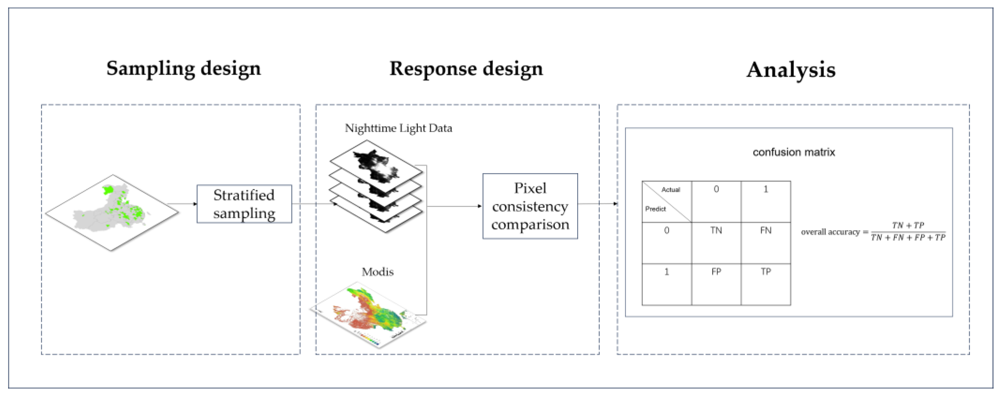
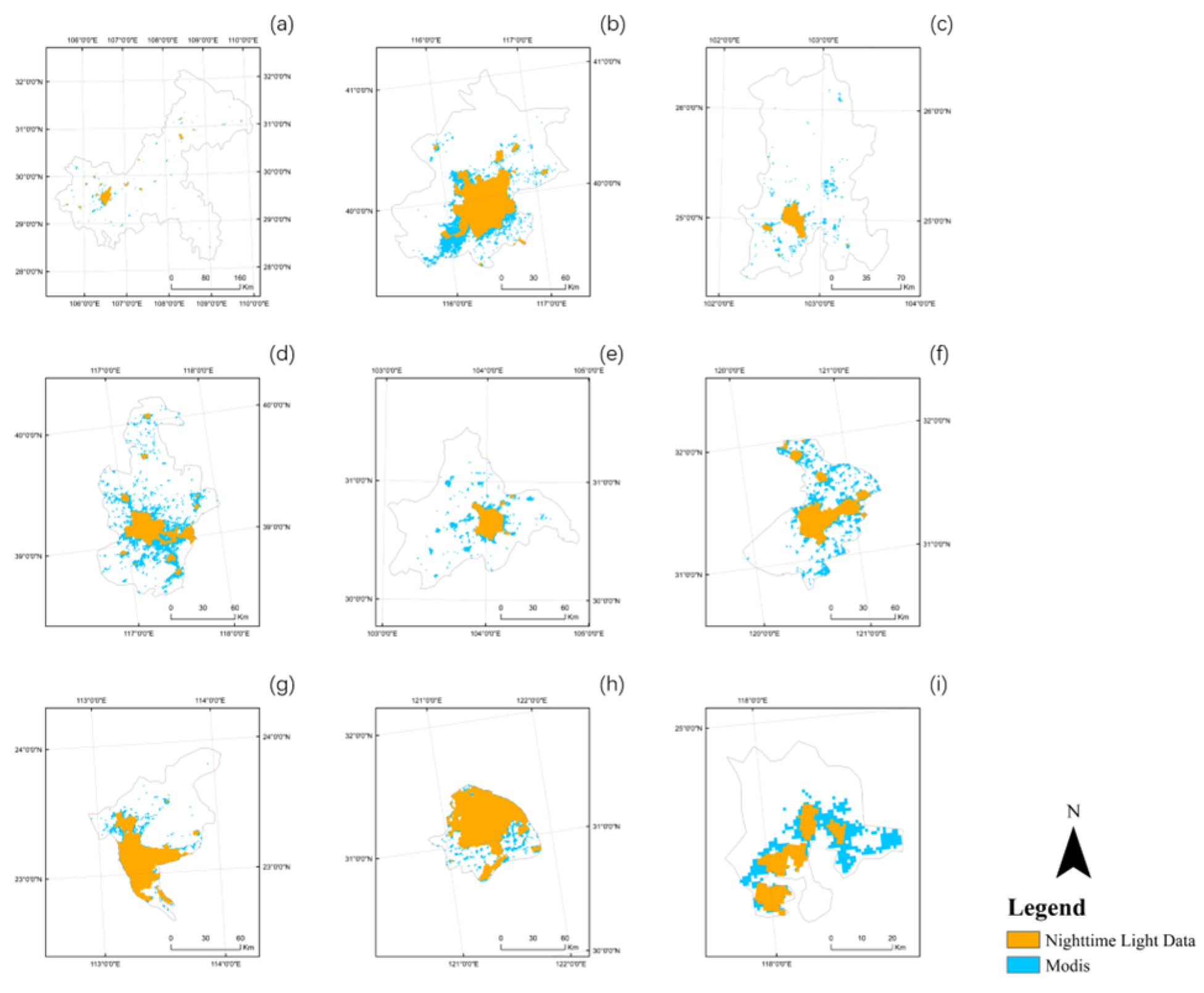
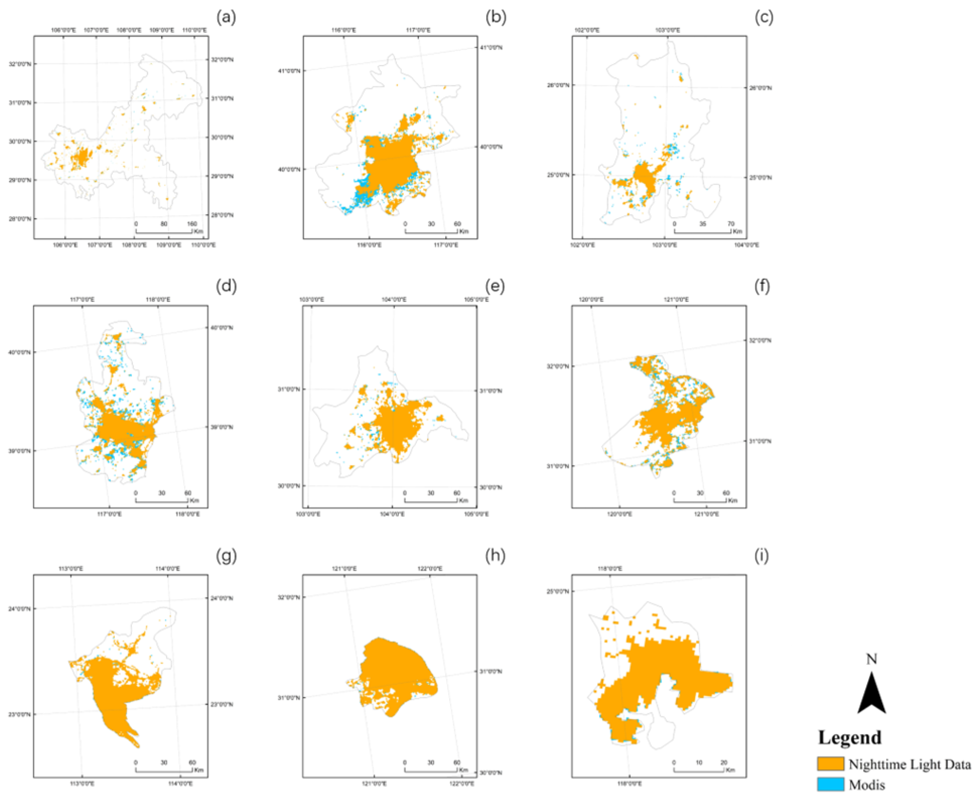
2.5. Validation for Urban Built-Up Area Extraction Results

According to the framework proposed by Olofsson et al., the good practice recommendations for assessing accuracy comprise three components: sampling design, response design, and analysis [54]. After extracting the built-up areas, this paper evaluates the accuracy of the results following the process (Figure 8).

For sampling design, simple random, stratified, and systematic sampling methods are commonly used in research [55]. Stratified random sampling is a probability sampling design that is relatively easy to implement and is widely used in the field of remote sensing for accuracy assessment [56]. In this study, a stratified sampling method is employed, categorizing 68 cities into three classes based on their area: large, medium, and small. Sampling is conducted within each category, resulting in the selection of nine cities for accuracy assessment. The nine cities selected are Chongqing, Beijing, and Kunming (large); Tianjin, Chengdu, and Suzhou (medium); and Guangzhou, Shanghai, and Xiamen (small).

For response design, the MCD12Q1 products of MODIS in 2010 and 2020 are used to as the reference data; these data are of a high quality and come from one of the most widely used land cover datasets globally. In this paper, the land cover class is selected and labeled as a built-up area from the MCD12Q1 product, and its consistency is compared with the built-up area pixels extracted in our study on a per-pixel basis.

For the analysis, the confusion matrix is used in this paper. The confusion matrix is a cross-tabulation method used to compare the class labels assigned by the remote sensing classification with the reference data for the sample sites, and it plays a central role in accuracy assessment [57]. The main diagonal of the confusion matrix displays correctly classified instances, while the off-diagonal elements represent misclassifications. The proportion of correctly classified pixels to the total number of pixels is referred to as the overall accuracy. A higher value indicates better classification performance [50]. In this study, the overall accuracy is used as a metric to evaluate the built-up area extraction results.

2.6. Methods for Factors Influencing Carbon Emissions

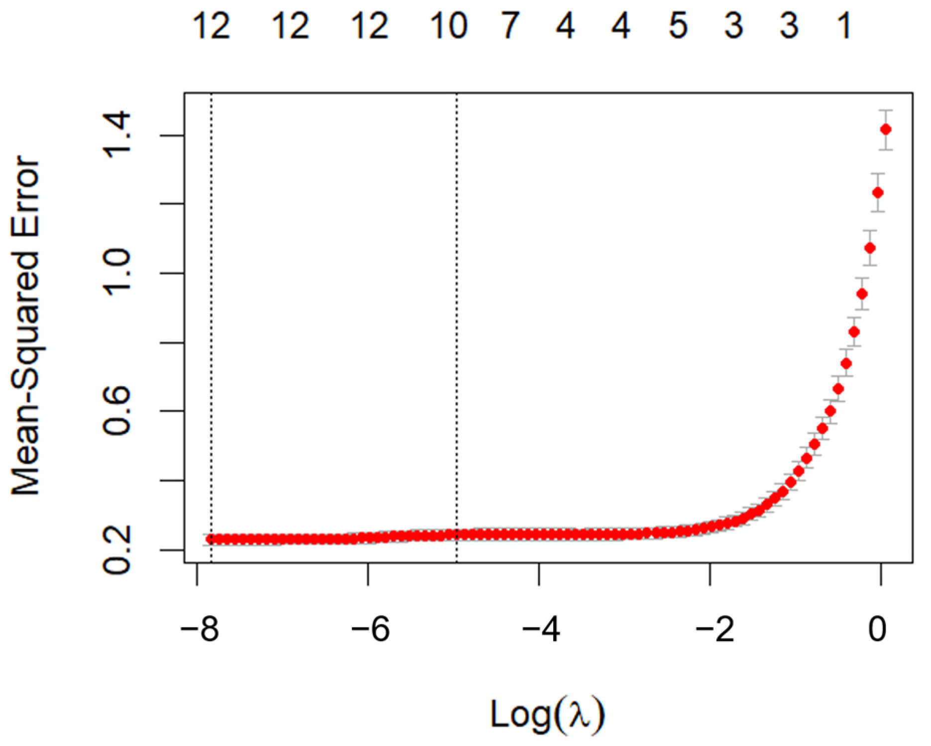
Based on the urban evaluation system established in the previous section, this article divides 68 cities into expansion and contraction types, selects socio-economic data related to carbon dioxide emissions (

Table 5. Data on factors influencing carbon emissions in low-carbon pilot cities.

ID	Meaning	Abbreviations
Y	Carbon emission	CE
X1	Population size	PS
X2	Employment numbers	EN
X3	GDP	GDP
X4	The proportion of tertiary industry	PTI
X5	Retail sales	RS
X6	Government investment	GI
X7	Built-up area	BA
X8	Built-up perimeter	BP
X9	Fractal dimension	FDI
X10	Compactness index	CI
X11	Virescence area	VA
X12	Nighttime light intensity	NLI

), and proposes a method to discuss the similarities and differences of carbon emission factors among different types of cities.

2.6.1. Lasso

In order to comprehensively consider influencing factors and increase the model’s interpretability, a large number of variables are usually chosen to be included in the model in research. However, as the number of variables increase, multicollinearity and variable autocorrelation will occur, which will reduce the accuracy of the model. The Lasso method is widely used to select variables. The Lasso method adds a penalty term to the model and adjusts it to affect the coefficients of the model. In this process, the coefficients of some insignificant variables will gradually approach 0. By deleting these variables, variable screening can be achieved. The specific implementation process is as follows [58]:

$Y$ is the dependent variable, $X$ is the independent variable, and the observed values of sample data are $(X, Y)$. The following linear relationship can be established between them. $\beta$ is the regression coefficient and $\epsilon$ is the random disturbance term.

$$Y=X\beta +\epsilon$$

(3)

To select significant variables, it is necessary to perform Lasso estimation on the unknown parameter $\beta$ in the above model. The estimated value of β must satisfy the minimum value of the following formula. $\lambda {\displaystyle \sum _{j=1}^p\left|{\beta }_j\right|}$ represents the penalty term. $\lambda \ge 0$ is an adjustment parameter, indicating the intensity of punishment. As $\lambda$ becomes larger, the penalty will increase, the selection of variables will become stricter, and some insignificant variables will be eliminated.

$${\widehat{\beta }}_{lasso}=\arg \min (||Y-X\beta |{|}^2+\lambda {\displaystyle \sum _{j=1}^P\left|{\beta }_j\right|)=RSS+}\lambda {\displaystyle \sum _{j=1}^P\left|{\beta }_j\right|}$$

(4)

Usually, the Lasso cross-validation (LassoCV) method can be used to adjust the values of the parameter $\lambda$. By selecting a range of $\lambda$ values, calculating the corresponding cross-validation errors, and choosing the parameter with the minimum CV error, the optimal tuning parameter value is determined. This article uses the K-fold cross validation method to select λ. The K-fold cross validation method divides the initial observation dataset into roughly identical K sub samples, selecting one as the validation set each time and the remaining K − 1 as the training set. The training is repeated K times, and the entire process will result in K test errors $MS{E}_1$,$MS{E}_2$, …, $MS{E}_i$.The cross validation error is as follows:

$$C{V}_{\left(K\right)}={\displaystyle \frac{1}{K}}{\displaystyle \sum _{i=1}^{K}MS{E}_i}$$

(5)

2.6.2. Hierarchical Regression Model

When analyzing the factors affecting carbon emissions, this article uses the hierarchical regression model. The hierarchical regression model is an effective method for analyzing the degree of influence of variables on dependent variables, as well as studying the relationship between different variables and dependent variables by analyzing the R-squared changes when variables are added at different levels [59,60].

$$\left\{\begin{array}{l}{Y}_{n,m}={\mathrm{\alpha }}_0+{\mathrm{\alpha }}_n{X}_{n,m}+{\epsilon }_i\\ Y_{n+1,m}={\mathrm{\alpha }}_0+{\mathrm{\alpha }}_n{X}_{n,m}+{\mathrm{\alpha }}_{n+1}{X}_{n+1,m}+{\epsilon }_i\\ Y_{n+2,m}={\mathrm{\alpha }}_0+{\mathrm{\alpha }}_n{X}_{n,m}+{\mathrm{\alpha }}_{n+1}{X}_{n+1,m}+{\mathrm{\alpha }}_{n+2}{X}_{n+2,m}+{\epsilon }_i\end{array}\right.$$

(6)

$Y_i$ is the carbon emissions of city $i$. ${\mathrm{\alpha }}_i$ is the regression coefficient for variable $X_i$. ${\epsilon }_i$ is the error term. $n$ and $m$ represent the number of regression steps and the type of city in hierarchical regression model, respectively. With the steps increasing by one, one more variable was added in the step $n+i$. The variables with significance and with a change in the R-square value were selected as independent variables to construct the specific regression model for this type of city.

3. Results

3.1. Extraction of Built-Up Areas

After extracting the boundaries of built-up areas, sample cities are selected, including Chengdu and Chongqing, and an accuracy assessment is conducted. The overall accuracy of urban area extraction ranges from a maximum of 98.87% to a minimum of 70.90% (

Table 6. The overall accuracy calculated during the accuracy assessment.

Number	City	Time	Overall Accuracy
(a)	Chongqing	2010	90.22%
		2020	88.76%
(b)	Beijing	2010	98.87%
		2020	97.27%
(c)	Kunming	2010	97.27%
		2020	95.05%
(d)	Tianjin	2010	85.53%
		2020	85.82%
(e)	Chengdu	2010	94.49%
		2020	86.18%
(f)	Suzhou	2010	82.73%
		2020	80.73%
(g)	Guangzhou	2010	89.12%
		2020	71.49%
(h)	Shanghai	2010	82.08%
		2020	71.49%
(i)	Xiamen	2010	79.33%
		2020	70.90%

). Therefore, it can be concluded that the extraction results using integrated nighttime light images meets the experimental requirements. Figure 9 and Figure 10 show a comparison of the built-up areas extracted from MODIS data and nighttime light data.

3.2. Result of Establishment of Urban Development Evaluation System

According to the urban development evaluation system established, with a time interval of 5 years, the subsystem scores and overall development scores for 68 cities are calculated and categorized. Next, the results are discussed in sequence based on the overall development of the 68 cities, followed by the development of the four subsystems: population, economy, construction, and society.

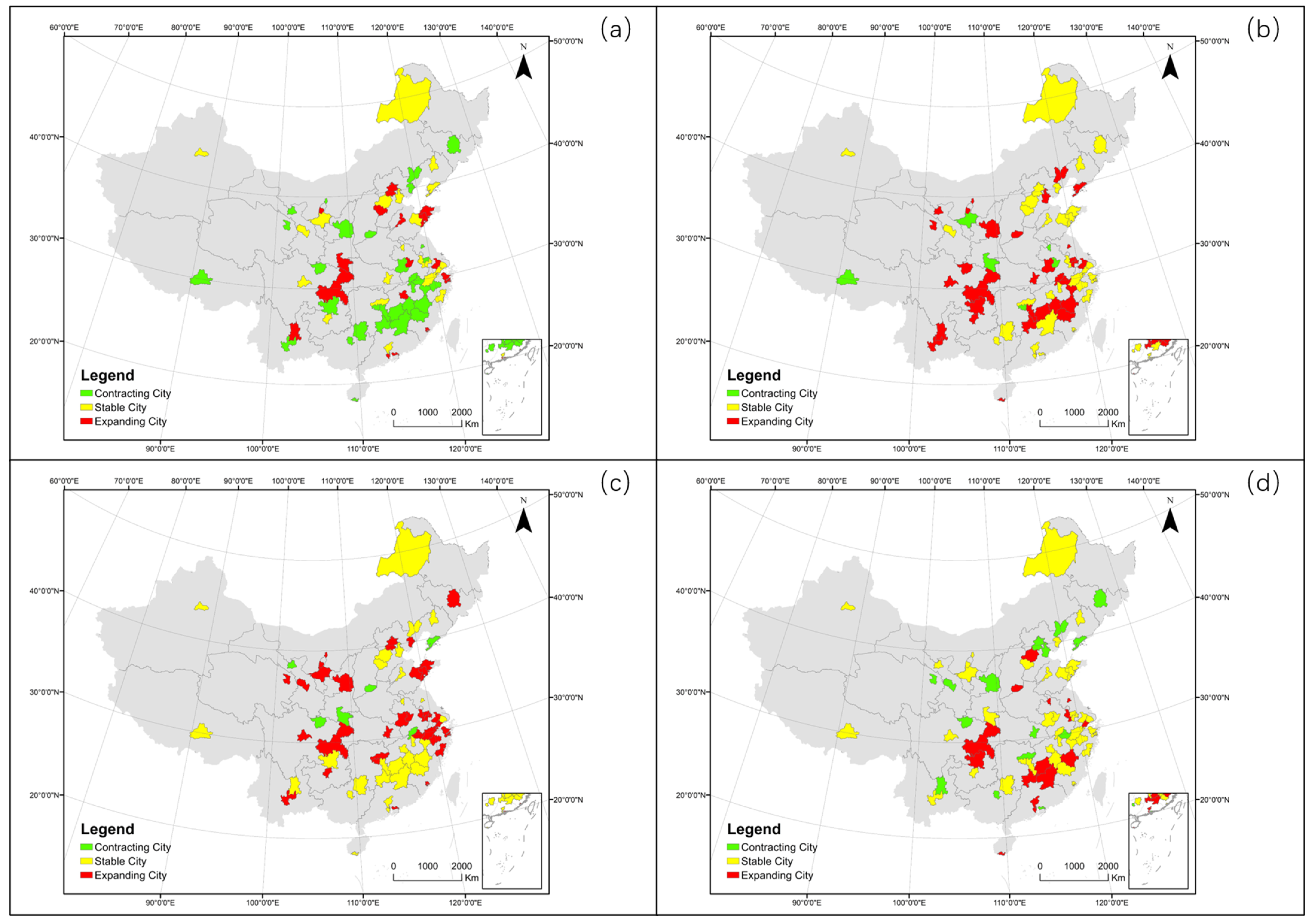
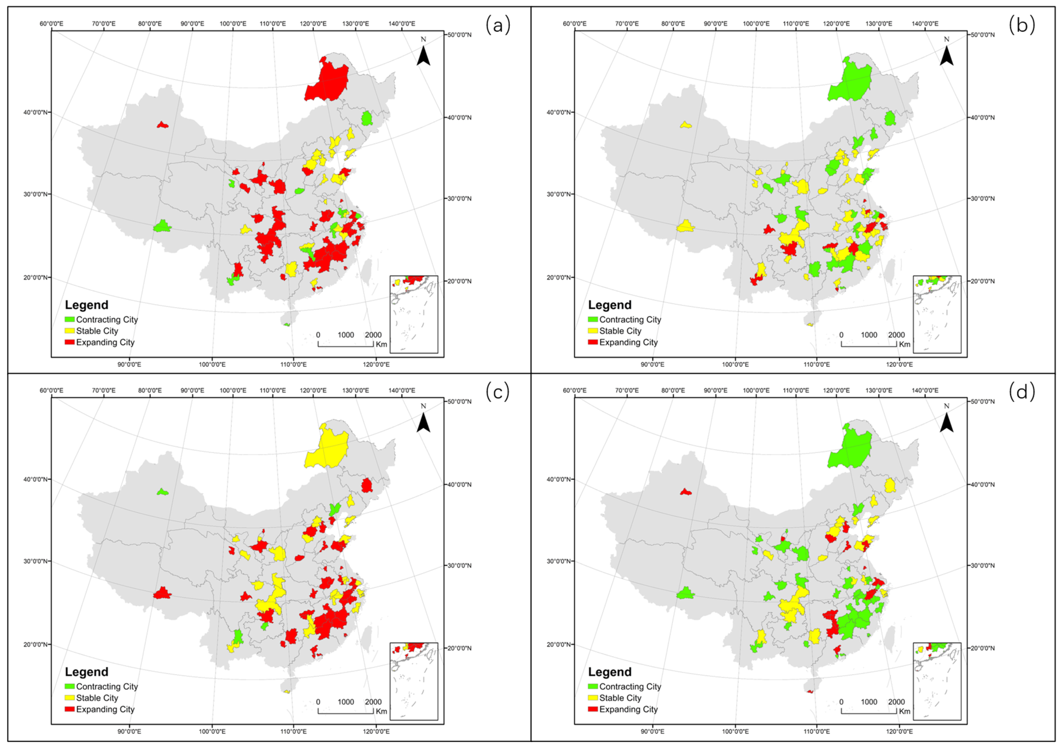
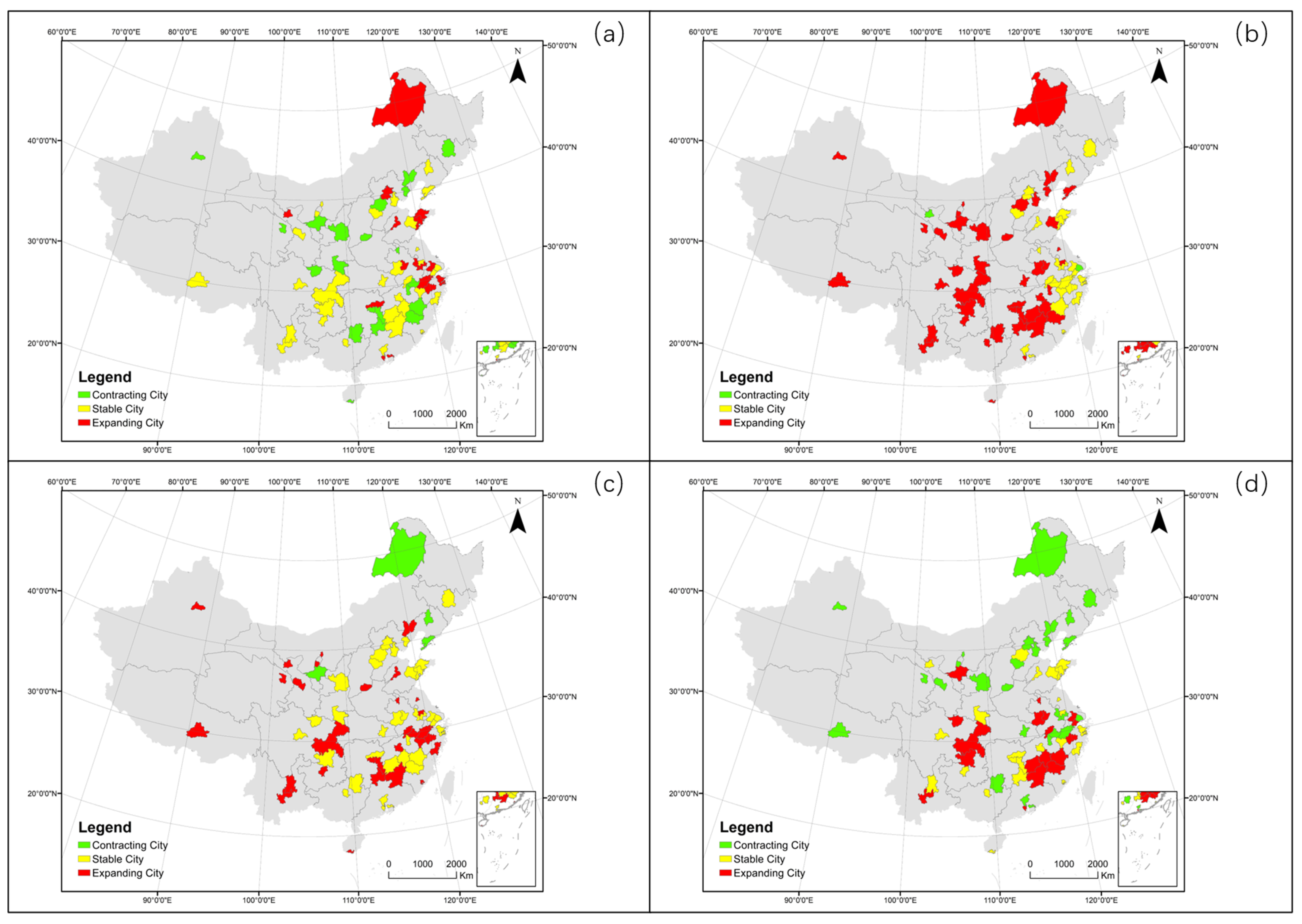
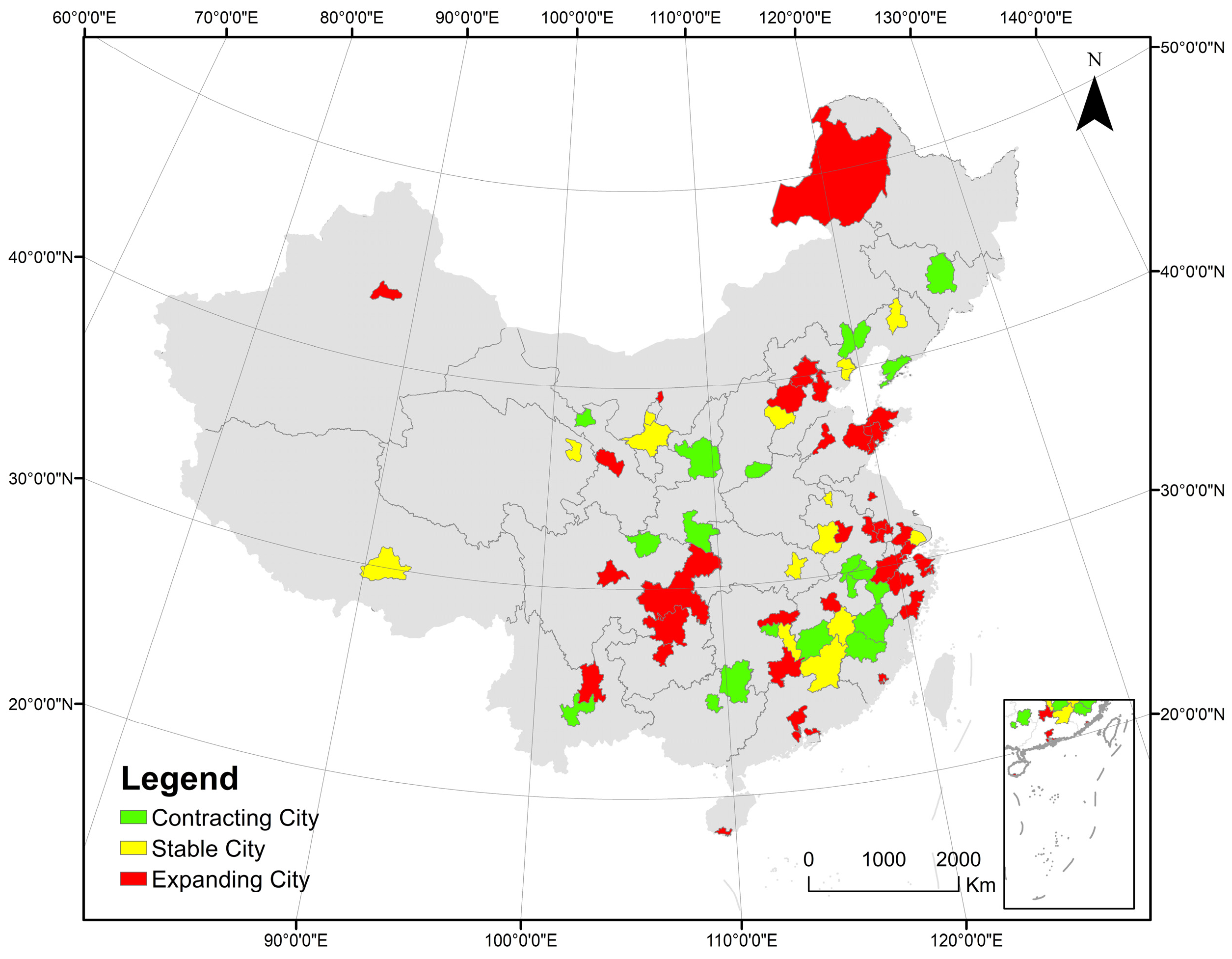
3.2.1. Overall Development of the 68 Cities

This section presents the overall development trends of 68 cities from 2002 to 2021.

Table 7. The number of cities with three development types (contracting city, stable city, and expanding city).

	2002–2006	2007–2011	2012–2016	2017–2021
Contracting City	31	6	6	15
Stable City	21	30	29	38
Expanding City	16	32	33	15

shows the number of cities of each type in four periods. In the first period (2002–2006), the development of 20 cities was stable. And in the fourth stage (2018–2021), it increased to 38. The number of expanding cities initially increases and then decreases, while it is opposite for contracting cities. In general, the development of urbanization will undergo a period of fluctuations and gradually reach a stable state.

Figure 11 shows the geographical distribution of different types of cities. Cities in the southeastern region, such as those in Jiangxi and Fujian provinces, exhibit synchronous development characteristics. Over the past 20 years, their development has undergone phases of contraction, followed by expansion and then stabilization. Some major cities, such as Beijing and Chongqing, have undergone more significant fluctuations in their development process. Meanwhile, cities in the northeastern and northwestern regions, such as Hulunbuir and Urumqi, have maintained a stable development pattern throughout the 20-year period. It can be seen that geographical location has a significant impact on urban development.

In the meantime, we classified cities based on the scores of each subsystem and counted their numbers (

Table 8. The number of three types of cities divided by subsystem scores.

		2002–2006	2007–2011	2012–2016	2017–2021
Population subsystem	Contracting City	13	22	4	35
	Stable City	18	35	25	17
	Expanding City	37	11	39	16
Economy subsystem	Contracting City	21	2	4	27
	Stable City	31	23	34	23
	Expanding City	16	43	30	18
Construction subsystem	Contracting City	49	9	21	7
	Stable City	14	20	25	35
	Expanding City	4	39	22	26
Society subsystem	Contracting City	9	14	7	25
	Stable City	15	27	5	15
	Expanding City	44	27	56	28

).

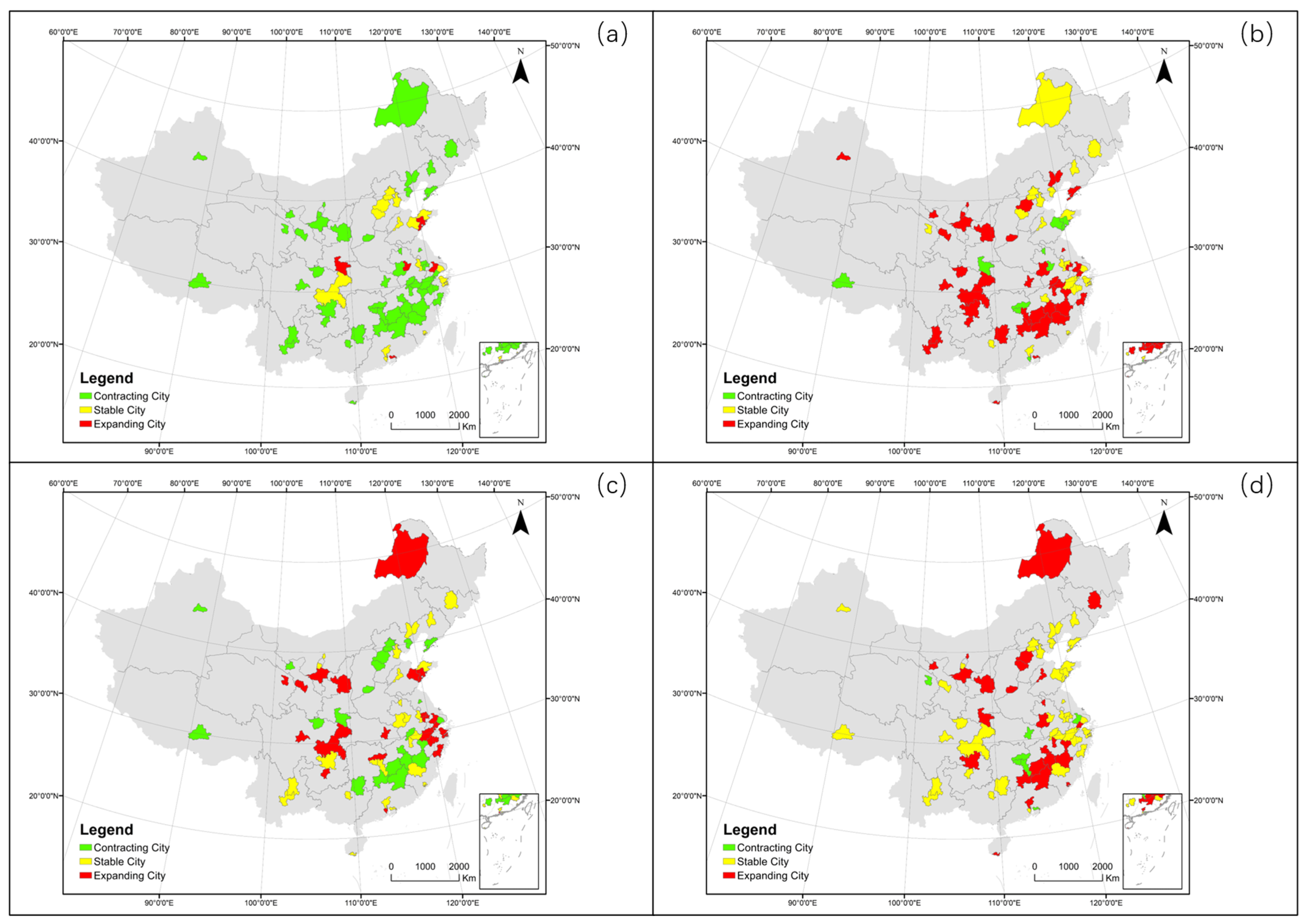
3.2.2. The Development of the Population Subsystem

This section presents the development trends of the population subsystems for 68 cities from 2002 to 2021.

Based on Figure 12, it can be observed that the population subsystem in Chinese cities exhibited an expansionary trend during the first phase (2002–2006) and the third phase (2012–2016). In contrast, a significant contraction occurred during the second phase (2007–2011) and the fourth phase (2017–2021). This indicates that the population subsystem tends to undergo a decline once it reaches a certain scale of development.

At the same time, the development of the population subsystem exhibits clear agglomeration characteristics. For example, cities in the southeastern regions, such as those in Jiangxi, Hunan, and Fujian Provinces, display similar patterns of change.

3.2.3. The Development of the Economy Subsystem

This section details the development of the economic subsystems for 68 cities from 2002 to 2021.

As shown in Figure 13, from 2002 to 2006, the cities with an expanding economic subsystem were mainly located in the coastal areas and the border areas. From 2007 to 2011, the economic subsystem of most cities underwent a concentrated expansion. After this period, cities with contracting economic subsystems were gradually concentrated northward, while expanding cities gradually moved southward. Overall, compared to cities in coastal regions, the economic subsystems of some resource-based cities in inland areas tend to be less stable, exhibiting more pronounced fluctuations between rapid economic growth and contraction.

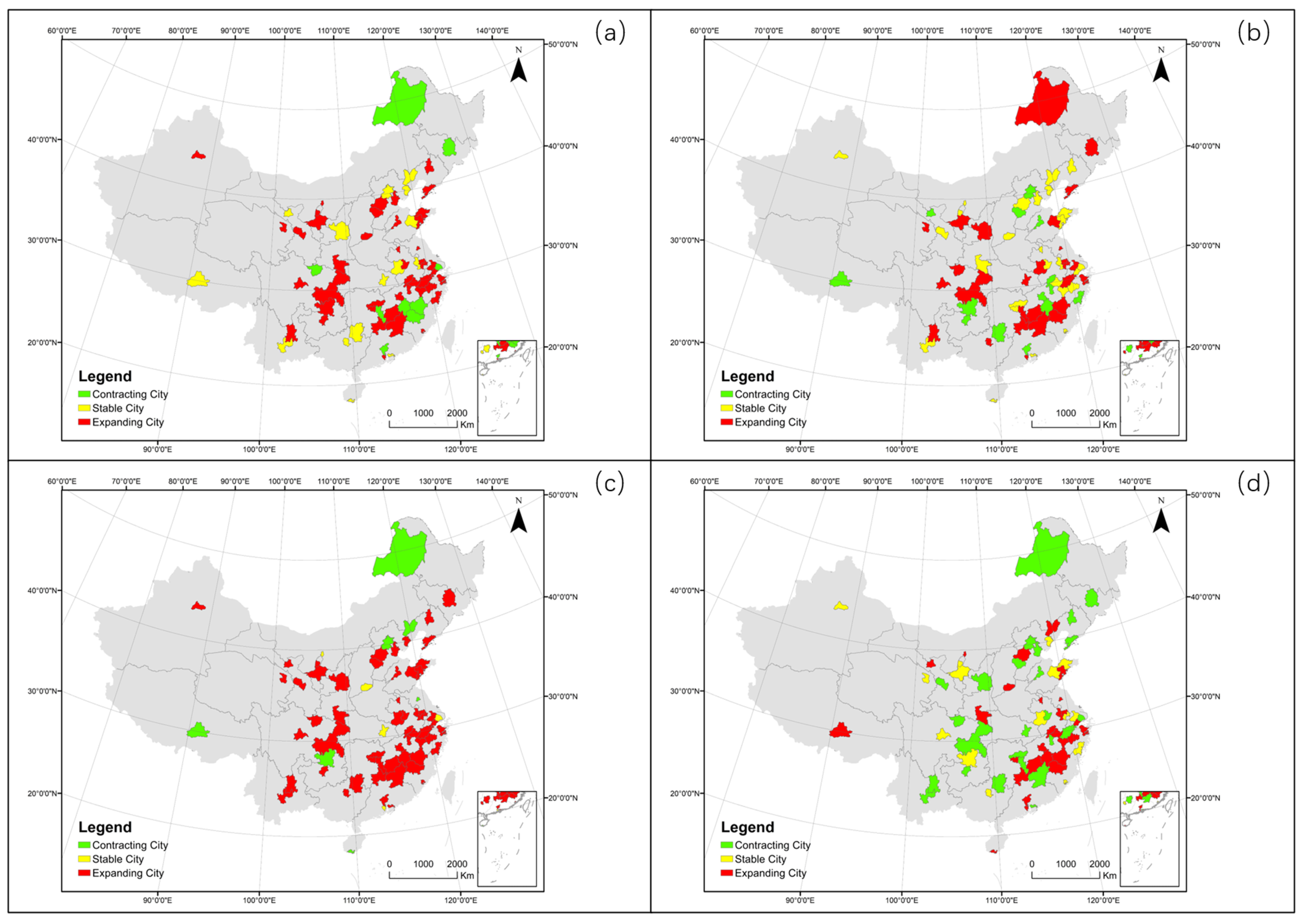
3.2.4. The Development of the Construction Subsystem

This section outlines the development of the construction subsystems across 68 cities from 2002 to 2021.

As illustrated in Figure 14, the development of the construction subsystem in Chinese cities was predominantly characterized by contraction during the first phase (2002–2006). Expansion began in the second phase (2007–2011) and subsequently approached a stable state. Overall, regions with more advanced economies tend to initiate urban construction earlier. Once the demand is met, the pace of construction gradually slows down, leading to an earlier stabilization.

3.2.5. The Development of the Society Subsystems

This section examines the development of the social subsystems for 68 cities from 2002 to 2021.

As Figure 15 shows, from 2002 to 2016, the society subsystem of the city was mainly expanding, with a number of 44, 27, and 56, respectively. In the meantime, the expanding society subsystem gradually spreads from south to north. Since 2017, the number of contracting society subsystems has begun to increase. The contracting society subsystem gradually spreads to inland areas. In general, the social subsystem of southern cities developed earlier than that of northern and western cities. The development of society subsystems in cities located in the southeast region has been in a relatively settled state of expansion.

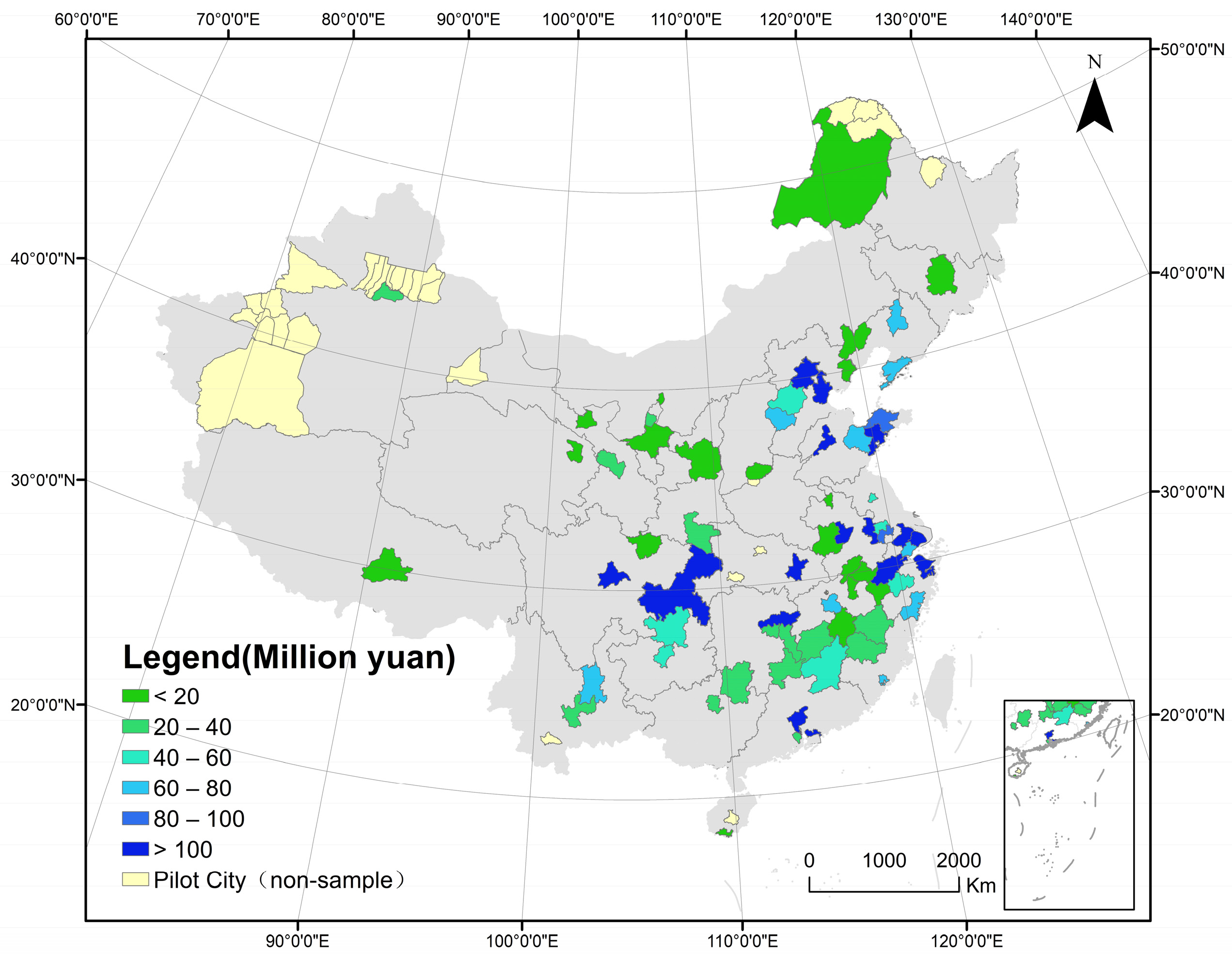
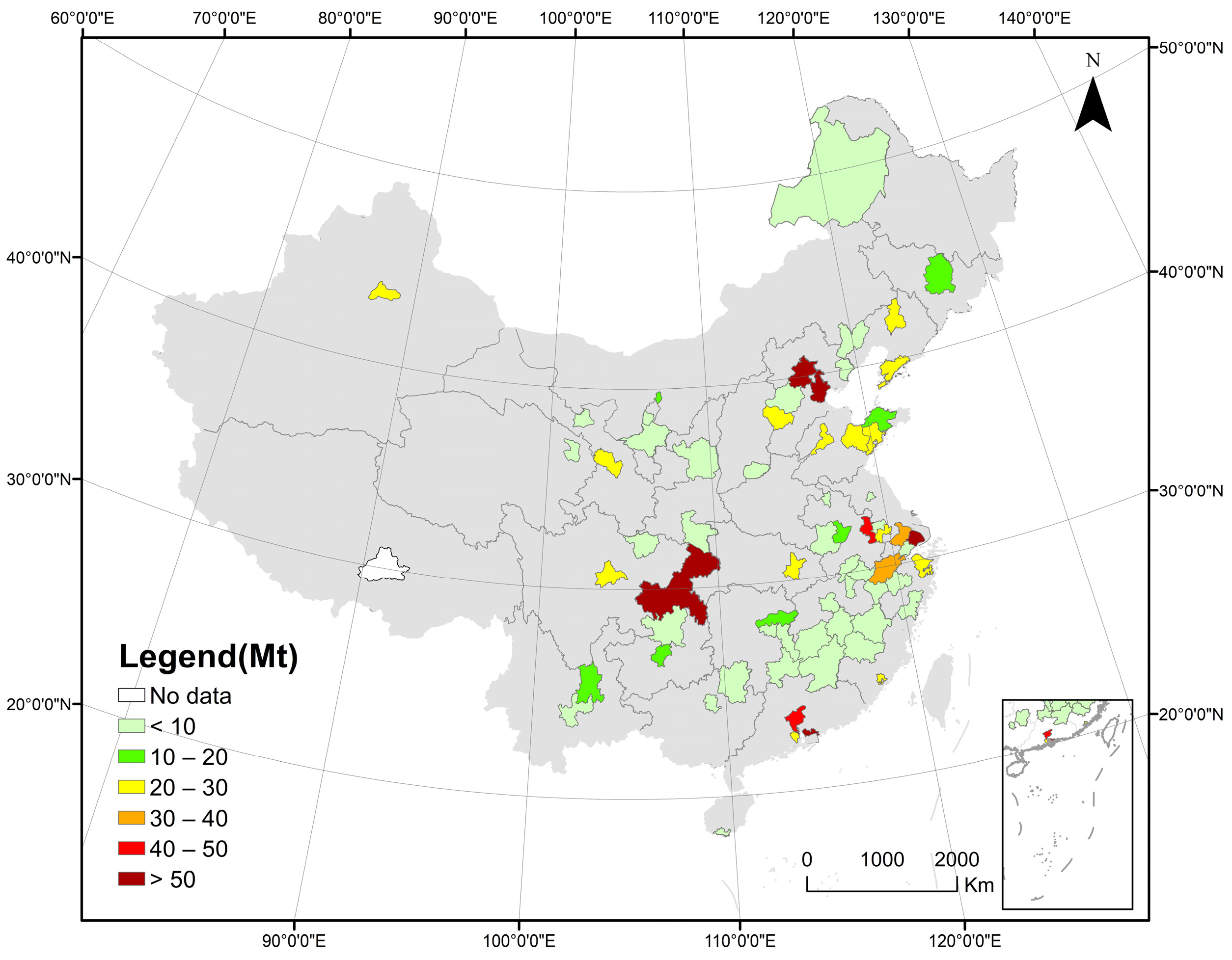
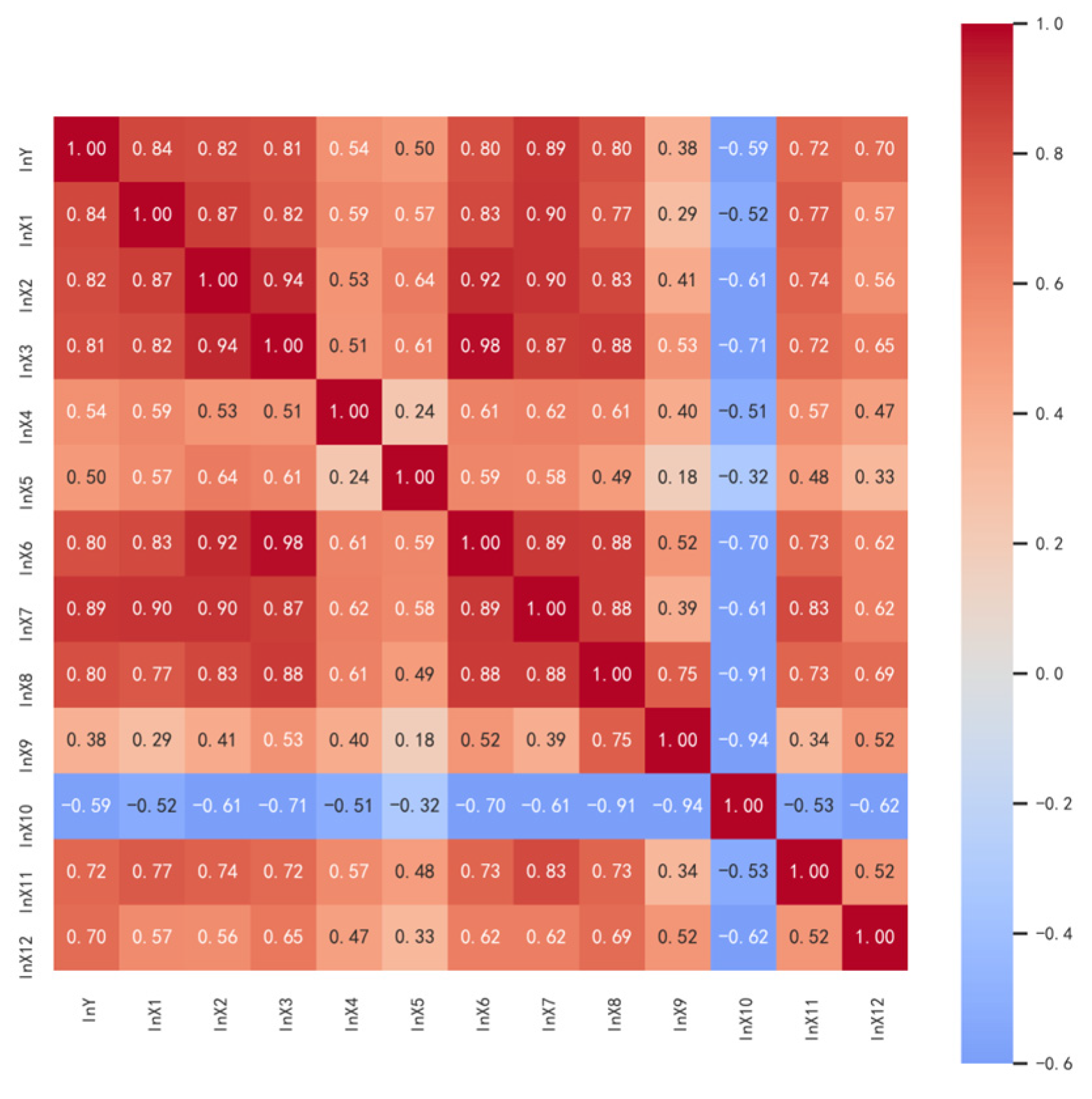
3.3. Influence Factor of CO₂

From 2006 to 2019, the average annual carbon emissions of 67 cities except Lhasa were 16.51 million tons. The spatial distribution of carbon emissions shows a characteristic of high in the east and low in the west (Figure 16). A total of 27 cities have average annual carbon emissions of less than 10 million tons (Mt). Cities with average annual carbon emissions of 10–30 Mt are mainly concentrated in the Liaodong Peninsula region. Cities with emissions exceeding 30 Mt are primarily concentrated in the eastern and southern regions, such as Suzhou, Hangzhou, Guangzhou, and Shenzhen. Additionally, four municipalities directly under the central government (Beijing, Shanghai, Chongqing, and Tianjin) have average annual carbon emissions exceeding 50 Mt.

According to the urban evaluation system established earlier, 68 cities from 2006 to 2019 were reclassified (Figure 17). A total of 19 cities are categorized as contracting cities, while 35 cities are classified as expanding cities. Contracting cities are primarily located in the central regions, such as Shanxi, Anhui, and Hunan province. Expanding cities are concentrated in the central and eastern regions, including the Beijing–Tianjin–Hebei urban agglomeration, the Chengdu–Chongqing metropolitan area, and the Yangtze River Delta urban cluster.

Before performing the regression analysis, Pearson correlation coefficients were used to measure the relationships between 12 influencing factors and carbon emissions. A correlation matrix was derived and visualized as a heatmap (Figure 18). To address potential issues arising from significant differences in carbon emissions and influencing factor data, all data were transformed using the natural logarithm to reduce variability.

The heatmap reveals that the absolute values of the correlation coefficients between carbon emissions and 12 influencing factors range from 0.39 to 0.89, indicating a high level of correlation. Additionally, the absolute values of correlation coefficients among most influencing factors are also quite high. For example, the correlation coefficient between government investment and GDP is 0.98. This suggests the presence of multicollinearity among the factors.

To assess multicollinearity, the Variance Inflation Factor (VIF) was used. Typically, a VIF value greater than 10 indicates the presence of multicollinearity. The calculation results are presented in

Table 9. Variance Inflation Factor (VIF) of factors.

Variable	VIF
X8	83.1233
X10	58.7077
X3	54.2692
X6	45.3954
X7	34.1285
X9	19.7756
X2	13.1348
X1	6.6273
X11	3.3523
X4	3.0207
X12	2.3542
X5	1.7763

. Seven variables have VIF values exceeding 10, indicating the presence of significant multicollinearity. Therefore, a further variable selection is necessary.

The Lasso method is used to reselect key factors influencing carbon emissions. When using the Lasso method to screen variables, one important step is to adjust the selection of parameter λ.

Table 10. The results of variable selection using the Lasso method.

	Df	%Dev	Lambda
1	0	0	1.062
2	1	13.49	0.9673
3	1	24.7	0.8814
…	…	…	…
53	9	83.63	0.01112
54	9	83.67	0.01013
55	9	83.69	0.00923
56	10	83.87	0.00636
57	10	83.91	0.0058
58	10	83.94	0.00528
59	11	83.97	0.00481
60	11	84.04	0.00439
61	11	84.09	0.004
62	12	84.2	0.00364
63	12	84.48	0.00276

shows the different results corresponding to different lambda values. $Df$ represents the degree of freedom of the model, and $\%Dev$ represents the degree of explanation of the residuals by the model. The larger the value, the better the fitting effect. It can be seen from the results in the table that the interpretability of the model continues to increase as $\lambda$ decreases, but its growth rate gradually slows down. Even if the $\lambda$ value keeps getting smaller and $Df$ keeps getting larger, the residual explanation ratio does not change much. Based on this, the number of independent variables in the model can be selected as 9 or 10.

To further select the optimal parameters, K-fold cross-validation is typically employed. Figure 19 shows the result of the K-fold cross-validation. The dashed line on the left represents the logarithmic value corresponding to the minimum root mean square error (RMSE), while the dashed line on the right indicates the logarithmic value at one standard deviation away from this minimum value. The numbers above the dashed lines indicate the corresponding number of variables. Generally, the solution corresponding to the right-hand dashed line is considered the optimal choice.

The selected λ is input into the Lasso cross-validation model, and the final results of variable selection are presented in

Table 11. Table of variable selection results.

Variable	Coefficient	Result
X1	0.2060	Reserve
X2	0.0444	Reserve
X3	0.0064	Reserve
X4	−0.1708	Reserve
X5	−0.0209	Reserve
X6	0.0000	Discard
X7	0.6569	Reserve
X8	0.0000	Discard
X9	0.3582	Reserve
X10	−0.0681	Reserve
X11	−0.0181	Reserve
X12	0.3143	Reserve

. The coefficients for variables X6 and X8 are zero and have been discarded, while the remaining nine variables are retained. This indicates that the retained variables have a significant impact on carbon emissions.

Next, based on the classification results presented, the similarities and differences in the factors influencing carbon emissions between expanding and contracting cities are further discussed.

Table 12. Results and analysis of hierarchical regressions in contracting cities.

	(1) lnY	(2) lnY	(3) lnY	(4) lnY	(5) lnY
lnX7	0.939 ***	0.848 ***	0.472 ***	0.696 ***	0.736 ***
	(33.677)	(32.079)	(8.034)	(7.387)	(7.804)
lnX12		0.300 ***	0.275 ***	0.290 ***	0.296 ***
		(10.015)	(8.848)	(9.413)	(9.688)
lnX1			0.429 ***	0.432 ***	0.459 ***
			(7.378)	(7.563)	(8.009)
lnX10				−0.777 ***	−0.777 **
				(−4.871)	(−4.781)
lnX4					−0.351 **
					(−2.912)
Constant	2.063 ***	1.791 ***	1.711 ***	3.163 ***	3.613 ***
	(13.438)	(12.866)	(12.406)	(7.646)	(7.646)
Observations	377	377	377	377	377
R-squared	0.752	0.803	0.826	0.828	0.837
F	240.592	136.907	97.007	77.144	63.469

*** p < 0.05, ** p < 0.1.

and

Table 13. Results and analysis of hierarchical regressions in expanding cities.

	(1) lnY	(2) lnY	(3) lnY	(4) lnY	(5) lnY
lnX7	0.949 ***	0.848 ***	0.627 ***	0.734 ***	0.543 ***
	(15.511)	(32.079)	(7.326)	(7.375)	(4.304)
lnX12		0.378 ***	0.414 ***	0.412 ***	0.519 ***
		(3.958)	(4.006)	(4.021)	(4.897)
lnX2			0.278	0.268 ***	0.373 ***
			(2.866)	(2.787)	(3.674)
lnX11				−0.104 **	−0.124 **
				(−0.258)	(−2.473)
lnX10					−1.733 ***
					(−3.006)
Constant	1.845 ***	2.048 ***	1.832 ***	1.595 ***	2.672 ***
	(7.353)	(8.270)	(7.305)	(5.821)	(6.393)
Observations	203	203	203	203	203
R-squared	0.738	0.760	0.783	0.788	0.801
F	240.592	136.907	78.558	64.720	50.016

*** p < 0.05, ** p < 0.1.

show the hierarchical regression results of two-type cities. As shown in the table, with the inclusion of additional variables, the R-squared value of the carbon emissions influence model for contracting cities reaches 0.801, while for expanding cities, it reaches 0.837. All variables in the models pass significance tests.

According to the regression results, a multiple linear regression model is established for the proportion of carbon emissions and related factors of two-type cities as follows.

$$\ln C{E}_{(contracting)}=0.543\ln BA+0.519\ln NLI+0.373\ln EN-0.124\ln VA-1.733\ln CI+2.672$$

(7)

$$\ln C{E}_{(Expanding)}=0.736\ln BA+0.296\ln NLI+0.459\ln PS-0.777\ln CI-0.531\ln PTI+3.613$$

(8)

The fitting results indicate that for both types of cities, built-up area, nighttime light intensity, and built-up area compactness are significant factors influencing carbon emissions. Specifically, built-up area and nighttime light intensity have a positive correlation with carbon emissions, while built-up area compactness has a negative correlation.

For contracting cities, employment numbers and virescence area also significantly impact carbon emissions. Employment numbers show a positive correlation, whereas green space area exhibits a negative correlation.

In expanding cities, the population size and the proportion of the tertiary sector are more influential. Population size is positively correlated with carbon emissions, while the proportion of the tertiary industry is negatively correlated with carbon emissions.

4. Discussion

4.1. Urbanization Development

Theories of urban contraction and expansion emerged in the latter half of the 20th century on a global scale. Scholars have employed changes in urban population size as the primary metric for assessing urban contraction and expansion [61,62]. With the study of urbanization processes, scholars have found that using a single indicator to evaluate urbanization processes can result in significant errors. Domestic and international research lacks a comprehensive assessment that integrates economic and social factors [63,64]. Therefore, our research offers an integrated evaluation of urban development from four dimensions—population, economy, construction, and society—extending existing theories of urban contraction and expansion.

Existing research suggests that “deindustrialization” is a primary cause of urban contraction [65]. The results of this study indicate that, over the past two decades, cities undergoing a significant contraction in China are predominantly traditional heavy industrial centers, such as Jilin, Wuhai, and Yan’an. Conversely, cities characterized by expansion are largely concentrated in regions such as the Yangtze River Delta and the Pearl River Delta, where the economy is primarily driven by the service sector and emerging industries. Additionally, the implementation of policies can have a significant impact on both urban expansion and contraction [66]. In 2008, the Chinese government proposed a policy named the Four Trillion Plan to address the global financial crisis and promote stable economic growth. Therefore, in the next five years, the economic subsystems of cities across the country will generally expand, and the direction of population subsystem expansion will also shift towards the east and south. This is also reflected in the results of this experiment. Additionally, the Beijing–Tianjin–Hebei region, the Yangtze River Delta, the Pearl River Delta, and the Chengdu–Chongqing metropolitan area, as major economic zones in China, exhibit a development pattern characterized by expansion from central cities outward. Consequently, cities situated at the center of these metropolitan areas are developed earlier and achieve stability sooner. The results of this paper also reveal that the development of urban construction subsystems follows the principle that earlier development leads to earlier stabilization. Furthermore, influenced by policies such as reform and opening-up policies, cities in the southern regions have prioritized development over those in the north, leading to an earlier expansion of the social subsystems in southern cities compared to their northern counterparts.

The expansion and contraction of cities also exhibit spatial distribution characteristics. Existing research shows that one pattern is the clustering of urban contraction and expansion; another pattern is that the expansion of central cities within metropolitan areas can induce contraction in surrounding cities [67,68]. According to the results of this paper, in southeastern China, the provinces of Jiangxi and Fujian, which share similar geographic conditions, undergo a significant interaction between their populations, leading to a flow of technology and economic activities. Within twenty years, urban development in this region has demonstrated synchronicity. This paper also indicates that, as core cities of the Chengdu–Chongqing metropolitan area, Chengdu and Chongqing attract population and resources from their surrounding areas, leading to contraction in neighboring cities such as Guangyuan, Zunyi, and Ankang.

The results of this study indicate that the expansion and contraction of cities are complex processes influenced by both the inherent attributes of cities and external factors such as policies and so on. In the meantime, these processes are closely linked to the development of surrounding cities.

4.2. Urbanization and Carbon Emissions

Current research on the relationship between urbanization and carbon emissions has explored various aspects, such as the impact of different stages of urbanization on carbon emissions and the effects of urbanization in different regions [69,70]. However, discussions on the factors influencing carbon emissions based on the expansion and contraction of urbanization are limited to smaller research scopes [71]. Therefore, the conclusions derived from this study contribute to the further development of theoretical frameworks and assist policymakers in formulating more effective carbon reduction strategies.

This study classifies 68 pilot cities into three types based on their development from 2006 to 2019 and compares the factors influencing carbon emissions in expanding and contracting cities. The results indicate that in both types of cities, an increase in built-up area and nighttime light intensity is associated with higher carbon emissions. Conversely, the compactness of the built-up area is negatively correlated with carbon emissions. Existing research suggests that urban expansion leads to an increased population, which in turn raises carbon emissions, and also results in higher energy consumption, further contributing to carbon emissions [72]. While a compact city model can reduce the residential energy consumption and the associated carbon emissions, urban expansion remains inevitable [73]. Thus, during urban development, it is crucial to avoid unchecked expansion, maintain a balance between humans and nature, and strive for optimal economic and social benefits [74,75].

In contracting cities, an increase in employment is associated with higher carbon emissions. According to previous analyses, most contracting cities in China are traditional industrial cities located in inland regions, where employment choices are predominantly industrial. In addition, the virescence area in contracting cities significantly impacts carbon emissions. Therefore, in contracting cities, it is essential to focus on environmental protection while considering industrial development, and to avoid issues such as excessive resource extraction [76].

In expanding cities, both population size and the proportion of the tertiary sector have a significant impact on carbon emissions. In China, expanding cities are largely concentrated in coastal areas, characterized by a service-oriented economy and a robust economic foundation, which attracts a substantial external population. Therefore, for expanding cities, policymakers should focus on how to balance the environmental pressures caused by the influx of the external population.

4.3. Limitations

Urbanization often leads to increased income for residents. On the one hand, higher income usually corresponds to a higher standard of living and greater consumption capacity, which can result in higher resource use and increased carbon emissions. On the other hand, higher income may also improve educational levels and enhance environmental awareness among residents [77,78]. Therefore, residents’ education and individual behavior are also crucial factors influencing carbon emissions. Future studies will aim to quantify residents’ psychological and behavioral characteristics to further explore the factors affecting carbon emissions from an individual perspective.

In constructing the urban development evaluation system, this paper chose the expansion of built-up areas as the primary indicator for the construction subsystem. Current research also incorporates additional metrics. For instance, the accessibility of urban transportation and the configuration of road networks can also serve as indicators for the progress of urbanization [79,80]. In future work, we will further refine the evaluation indicators to ensure that the evaluation system can more comprehensively assess urban development.

4.4. The Socio-Ecological Implications of the Results

From a socio-ecological perspective, the result indicates that while deindustrialized cities are undergoing an economic decline, service-oriented urban areas are seeing strong growth. This highlights the need for effective policies to support the economic transition of contracting cities, ensuring that they adapt sustainably and do not exacerbate social inequalities. Interactions between cities at the center of metropolitan areas and their surrounding cities illustrate the interconnected nature of urban development. This interconnectedness necessitates comprehensive regional planning that considers the wide-ranging impacts of expansion and contraction in central cities on surrounding areas. Policymakers should account for these dynamics to ensure equitable development across different regions.

Additionally, the study indicates that increases in built-up areas and energy consumption are key drivers of rising carbon emissions. Furthermore, issues related to population movement and environmental degradation also require significant attention. Therefore, governments should implement tailored low-carbon policies based on the development patterns and progress of different cities. For expanding cities, this involves integrating sustainable practices and resource efficiency. In contrast, contracting cities must prioritize environmental restoration and sustainable industrial practices.

Overall, this paper emphasizes the need for a multi-layered approach in urban policy development. On the one hand, a thorough understanding of the mechanisms driving urban growth can significantly enhance urban planning practices. By analyzing these mechanisms, planners can anticipate future challenges and opportunities and develop more forward-looking and adaptive policies. On the other hand, governments must consider both internal city factors and dynamic interactions with neighboring cities. Leveraging the advantages of developed cities to support surrounding areas is crucial for achieving regional balanced development. Policies that encourage inter-city cooperation and resource sharing can strengthen regional cohesion and promote sustainable urban growth.

5. Conclusions

This paper integrates two types of nighttime light data to create a long-term dataset of built-up areas in China from 2002 to 2021. Compared with MODIS land use data, the accuracy of the method exceeds 70%, demonstrating its effectiveness. By combining these data with social statistics, an evaluation system for urbanization development is established.

The analysis of urbanization development in 68 low-carbon pilot cities reveals that, over the past 20 years, most cities have undergone stable growth and are geographically concentrated. In contrast, cities with significant development fluctuations are more dispersed. These differences are influenced by internal city attributes, external policy factors, and the development of neighboring cities.

Regarding the factors influencing carbon emissions, the built-up area and nighttime light intensity exert a significant effect on carbon emissions across all city types. In contracting cities, employment numbers and virescence areas are significant, whereas, in expanding cities, population size and the proportion of the tertiary sector are more influential.

The study indicates that stable urban growth can lead to predictable carbon emissions and emphasizes the need for tailored policy approaches based on specific city characteristics. Future research should focus on longitudinal studies of urbanization trends, the impact of specific policies on development and emissions, and comparative studies in other regions to evaluate the generalizability of these findings. This paper aims to enrich our understanding of urbanization and its environmental impacts, inspiring further exploration into low-carbon development strategies and contributing to the theoretical foundations of urban studies.

References

1. Morikawa, H. Urbanization and Urban System; Damingtang Press: Hangzhou, China, 1989. [Google Scholar]
2. Liu, R.; Wang, M.; Chen, W. The influence of urbanization on organic carbon sequestration and cycling in soils of Beijing. Landsc. Urban Plan. 2018, 169, 241–249. [Google Scholar] [CrossRef]
3. Zhang, W.; Huang, B.; Luo, D. Effects of land use and transportation on carbon sources and carbon sinks: A case study in Shenzhen, China. Landsc. Urban Plan. 2014, 122, 175–185. [Google Scholar] [CrossRef]
4. Anderson, W. Urban form, energy and the environment: A review of issues, evidence and policy. Urban Stud. 1996, 33, 7–36. [Google Scholar] [CrossRef]
5. Shahbaz, M.; Sbia, R.; Hamdi, H.; Ozturk, I. Economic growth, electricity consumption, urbanization and environmental degradation relationship in United Arab Emirates. Ecol. Indic. 2014, 45, 622–631. [Google Scholar] [CrossRef]
6. Hao, Y.; Zhang, Z.-Y.; Liao, H.; Wei, Y.-M.; Wang, S. Is CO2 emission a side effect of financial development? An empirical analysis for China. Environ. Sci. Pollut. Res. 2016, 23, 21041–21057. [Google Scholar] [CrossRef]
7. Sadorsky, P. The effect of urbanization on CO2 emissions in emerging economies. Energy Econ. 2014, 41, 147–153. [Google Scholar] [CrossRef]
8. Wang, S.; Fang, C.; Guan, X.; Pang, B.; Ma, H. Urbanisation, energy consumption, and carbon dioxide emissions in China: A panel data analysis of China’s provinces. Appl. Energy 2014, 136, 738–749. [Google Scholar] [CrossRef]
9. Parikh, J.; Shukla, V. Urbanization, energy use and greenhouse effects in economic development. Glob. Environ. Chang. 1995, 5, 87–103. [Google Scholar] [CrossRef]
10. Gam, I.; Ben Rejeb, J. Electricity demand in Tunisia. Energy Policy 2012, 45, 714–720. [Google Scholar] [CrossRef]
11. Mishra, V.; Sharma, S.; Smyth, R. Are fluctuations in energy consumption per capita transitory? Evidence from a panel of Pacific Island countries. Energy Policy 2009, 37, 2318–2326. [Google Scholar] [CrossRef]
12. Martínez-Zarzoso, I.; Maruotti, A. The impact of urbanization on CO2 emissions: Evidence from developing countries. Ecol. Econ. 2011, 70, 1344–1353. [Google Scholar] [CrossRef]
13. Shafiei, S.; Salim, R.A. Non-renewable and renewable energy consumption and CO2 emissions in OECD countries: A comparative analysis. Energy Policy 2014, 66, 547–556. [Google Scholar] [CrossRef]
14. Xu, L.; Qu, J.; Li, H.; Zeng, J.; Zhang, H. Analysis and forecasting of carbon emissions from residential energy consumption in China. Ecol. Econ. 2019, 35, 19–23, 29. [Google Scholar]
15. Xue, B.; Li, C.; Liu, Z.; Geng, Y.; Xi, F. Analysis of the relationship between global carbon emissions and urbanization from 1970 to 2007. Adv. Clim. Chang. Res. 2011, 7, 423–427. [Google Scholar]
16. Cai, B.; Guo, H.; Cao, L.; Guan, D.; Bai, H. Local strategies for China’s carbon mitigation: An investigation of chinese city-level CO2 emissions. J. Clean. Prod. 2018, 178, 890–902. [Google Scholar] [CrossRef]
17. Li, H.; Qi, Y. Comparative scenarios of carbon emissions in China by 2050. Adv. Clim. Chang. Res. 2011, 7, 271–280. [Google Scholar]
18. Yang, M.; Guo, X.; Wu, L. Combined Land-Use and Transportation Demand Modeling Based on Equitableness. In Proceedings of the 2008 Workshop on Power Electronics and Intelligent Transportation System, Guangzhou, China, 2–3 August 2008; pp. 505–510. [Google Scholar] [CrossRef]
19. Dhakal, S. Urban energy use and carbon emissions from cities in China and policy implications. Energy Policy 2009, 37, 4208–4219. [Google Scholar] [CrossRef]
20. Zhang, X.-P.; Cheng, X.-M. Energy consumption, carbon emissions, and economic growth in China. Ecol. Econ. 2009, 68, 2706–2712. [Google Scholar] [CrossRef]
21. Wang, Y.; Luo, X.; Chen, W.; Zhao, M.; Wang, B. Exploring the spatial effect of urbanization on multi-sectoral CO2 emissions in China. Atmos. Pollut. Res. 2019, 10, 1610–1620. [Google Scholar] [CrossRef]
22. Pan, W. What type of mixed-use and open? A critical environmental analysis of three neighborhood types in China and insights for sustainable urban planning. Landsc. Urban Plan. 2021, 216, 104221. [Google Scholar] [CrossRef]
23. Li, H.; Peng, J.; Yanxu, L.; Yi’na, H. Urbanization impact on landscape patterns in Beijing City, China: A spatial heterogeneity perspective. Ecol. Indic. 2017, 82, 50–60. [Google Scholar] [CrossRef]
24. Liddle, B.; Lung, S. Age-structure, urbanization, and climate change in developed countries: Revisiting STIRPAT for disaggregated population and consumption-related environmental impacts. Popul. Environ. 2010, 31, 317–343. [Google Scholar] [CrossRef]
25. Qi, X.; Han, Y.; Kou, P. Population urbanization, trade openness and carbon emissions: An empirical analysis based on China. Air Qual. Atmos. Health 2020, 13, 519–528. [Google Scholar] [CrossRef]
26. Gurney, K.R.; Romero-Lankao, P.; Seto, K.C.; Hutyra, L.R.; Duren, R.; Kennedy, C.; Grimm, N.B.; Ehleringer, J.R.; Marcotullio, P.; Hughes, S.; et al. Climate change: Track urban emissions on a human scale. Nature 2015, 525, 179–181. [Google Scholar] [CrossRef] [PubMed]
27. Wang, C.-H.; Chen, N.; Chan, S.-L. A gravity model integrating high-speed rail and seismic-hazard mitigation through land-use planning: Application to California development. Habitat Int. 2017, 62, 51–61. [Google Scholar] [CrossRef]
28. Aunan, K.; Wang, S. Internal migration and urbanization in China: Impacts on population exposure to household air pollution (2000–2010). Sci. Total Environ. 2014, 481, 186–195. [Google Scholar] [CrossRef]
29. Dong, Y.; Yang, C.; Liu, X. The Exploration of China New Urbanization Theory. Urban Stud. 2017, 24, 26–34. [Google Scholar]
30. Zhou, C.; Wang, S.; Wang, J. Examining the influences of urbanization on carbon dioxide emissions in the Yangtze River Delta, China: Kuznets curve relationship. Sci. Total Environ. 2019, 675, 472–482. [Google Scholar] [CrossRef]
31. Wu, W.; Tan, W.; Wang, R.; Chen, W.Y. From quantity to quality: Effects of urban greenness on life satisfaction and social inequality. Landsc. Urban Plan. 2023, 238, 104843. [Google Scholar] [CrossRef]
32. Wang, C.; Wang, F.; Zhang, X.; Zhang, H. Influencing mechanism of energy-related carbon emissions in Xinjiang based on the input-output and structural decomposition analysis. J. Geogr. Sci. 2017, 27, 365–384. [Google Scholar] [CrossRef]
33. Baiocchi, G.; Minx, J.; Hubacek, K. The Impact of Social Factors and Consumer Behavior on Carbon Dioxide Emissions in the United Kingdom: A Regression Based on Input−Output and Geodemographic Consumer Segmentation Data. J. Ind. Ecol. 2010, 14, 50–72. [Google Scholar] [CrossRef]
34. Xu, Q.; Dong, Y.; Yang, R. Urbanization impact on carbon emissions in the Pearl River Delta region: Kuznets curve relationships. J. Clean. Prod. 2018, 180, 514–523. [Google Scholar] [CrossRef]
35. Elvidge, C.; Ziskin, D.; Baugh, K.; Tuttle, B.; Ghosh, T.; Pack, D.; Erwin, E.; Zhizhin, M. A Fifteen Year Record of Global Natural Gas Flaring Derived from Satellite Data. Energies 2009, 2, 595–622. [Google Scholar] [CrossRef]
36. Stewart, B.; Addison, D. Nighttime Lights Revisited: The Use of Nighttime Lights Data as a Proxy for Economic Variables; The World Bank Group: Washington, DC, USA, 2015. [Google Scholar] [CrossRef]
37. Yin, Z.; Li, X.; Tong, F.; Li, Z.; Jendryke, M. Mapping urban expansion using night-time light images from Luojia1-01 and International Space Station. Int. J. Remote Sens. 2020, 41, 2603–2623. [Google Scholar] [CrossRef]
38. Wang, L.; Jia, Y.; Li, X.; Gong, P. Analysing the Driving Forces and Environmental Effects of Urban Expansion by Mapping the Speed and Acceleration of Built-Up Areas in China between 1978 and 2017. Remote Sens. 2020, 12, 3929. [Google Scholar] [CrossRef]
39. Chen, Z.; Yu, B.; Song, W.; Liu, H.; Wu, Q.; Shi, K.; Wu, J. A New Approach for Detecting Urban Centers and Their Spatial Structure With Nighttime Light Remote Sensing. IEEE Trans. Geosci. Remote Sens. 2017, 55, 6305–6319. [Google Scholar] [CrossRef]
40. Ye, Y.; Yun, G.; He, Y.; Lin, R.; He, T.; Qian, Z. Spatiotemporal Characteristics of Urbanization in the Taiwan Strait Based on Nighttime Light Data from 1992 to 2020. Remote Sens. 2023, 15, 3226. [Google Scholar] [CrossRef]
41. Lu, C.; Li, L.; Lei, Y.; Ren, C.; Su, Y.; Huang, Y.; Chen, Y.; Lei, S.; Fu, W. Coupling Coordination Relationship between Urban Sprawl and Urbanization Quality in the West Taiwan Strait Urban Agglomeration, China: Observation and Analysis from DMSP/OLS Nighttime Light Imagery and Panel Data. Remote Sens. 2020, 12, 3217. [Google Scholar] [CrossRef]
42. Shan, Y.; Guan, D.; Liu, J.; Mi, Z.; Liu, Z.; Liu, J.; Schroeder, H.; Cai, B.; Chen, Y.; Shao, S.; et al. Methodology and applications of city level CO2 emission accounts in China. J. Clean. Prod. 2017, 161, 1215–1225. [Google Scholar] [CrossRef]
43. Shan, Y.; Guan, Y.; Hang, Y.; Zheng, H.; Li, Y.; Guan, D.; Li, J.; Zhou, Y.; Li, L.; Hubacek, K. City-level emission peak and drivers in China. Sci. Bull. 2022, 67, 1910–1920. [Google Scholar] [CrossRef]
44. Shan, Y.; Liu, J.; Liu, Z.; Shao, S.; Guan, D. An emissions-socioeconomic inventory of Chinese cities. Sci. Data 2019, 6, 190027. [Google Scholar] [CrossRef] [PubMed]
45. Peng, J.; Tian, L.; Liu, Y.; Zhao, M.; Hu, Y.; Wu, J. Ecosystem services response to urbanization in metropolitan areas: Thresholds identification. Sci. Total Environ. 2017, 607–608, 706–714. [Google Scholar] [CrossRef] [PubMed]
46. Friedmann, J. Four Theses in the Study of China’s Urbanization. Int. J. Urban Reg. Res. 2006, 30, 440–451. [Google Scholar] [CrossRef]
47. Tian, Y.; Tsendbazar, N.-E.; van Leeuwen, E.; Fensholt, R.; Herold, M. A global analysis of multifaceted urbanization patterns using Earth Observation data from 1975 to 2015. Landsc. Urban Plan. 2022, 219, 104316. [Google Scholar] [CrossRef]
48. Zhang, S.; Li, X.; Shi, Y. Spatial expansion of urban built-up areas in Zhengzhou based on GIS and its influencing factors. Henan Sci. 2017, 35, 1883–1888. [Google Scholar] [CrossRef]
49. Yang, X.; Liu, X.; Wang, R.; Liu, S. Evaluation of sustainable urbanization status in the Yangtze River Economic Belt. Resour. Dev. Mark. 2023, 39, 188–198. [Google Scholar]
50. Yu, M.; Guo, S.; Guan, Y.; Cai, D.; Zhang, C.; Fraedrich, K.; Liao, Z.; Zhang, X.; Tian, Z. Spatiotemporal heterogeneity analysis of yangtze river delta urban agglomeration: Evidence from nighttime light data (2001–2019). Remote Sens. 2021, 13, 1235. [Google Scholar] [CrossRef]
51. Zhao, M.; Zhou, Y.; Li, X.; Zhou, C.; Cheng, W.; Li, M.; Huang, K. Building a Series of Consistent Night-Time Light Data (1992–2018) in Southeast Asia by Integrating DMSP-OLS and NPP-VIIRS. IEEE Trans. Geosci. Remote Sens. 2020, 58, 1843–1856. [Google Scholar] [CrossRef]
52. Li, X.; Xu, H.; Chen, X.; Li, C. Potential of NPP-VIIRS Nighttime Light Imagery for Modeling the Regional Economy of China. Remote Sens. 2013, 5, 3057–3081. [Google Scholar] [CrossRef]
53. Imhoff, M. Using nighttime DMSP/OLS images of city lights to estimate the impact of urban land use on soil resources in the United States. Remote Sens. Environ. 1997, 59, 105–117. [Google Scholar] [CrossRef]
54. Olofsson, P.; Foody, G.M.; Herold, M.; Woodcock, S.V.S.C.E.; Wulder, M.A. Good practices for estimating area and assessing accuracy of land change. Remote Sens. Environ. Interdiscip. J. 2014, 148, 42–57. [Google Scholar] [CrossRef]
55. Stehman, S.V.; Selkowitz, D.J. A spatially stratified, multi-stage cluster sampling design for assessing accuracy of the alaska (USA) national land cover database (NLCD). Int. J. Remote Sens. 2010, 31, 1877–1896. [Google Scholar] [CrossRef]
56. Cakir, H.I.; Khorram, S.; Sac, N. Correspondence analysis for detecting land cover change. Remote Sens. Environ. Interdiscip. J. 2006, 102, 306–317. [Google Scholar] [CrossRef]
57. Stehman, S.V. Estimating area from an accuracy assessment error matrix. Remote Sens. Environ. 2013, 132, 202–211. [Google Scholar] [CrossRef]
58. Zhao, J.; Li, J.; Wang, P.; Hou, G. Research on the carbon peak path of Henan Province based on the Lasso-BP neural network model. Environ. Eng. 2022, 40, 151–156. [Google Scholar]
59. Chikán, A.; Czakó, E.; Kiss-Dobronyi, B.; Losonci, D. Firm competitiveness: A general model and a manufacturing application. Int. J. Prod. Econ. 2022, 243, 108316. [Google Scholar] [CrossRef]
60. Zheng, W.; Xu, X.; Wang, H. Regional logistics efficiency and performance in China along the Belt and Road Initiative: The analysis of integrated DEA and hierarchical regression with carbon constraint. J. Clean. Prod. 2020, 276, 123649. [Google Scholar] [CrossRef]
61. Joseph, S.; Jonathan, L. Greening the rust belt: A green infrastructure model for right sizing america’s shrinking cities. J. Am. Plan. Assoc. 2008, 74, 451–466. [Google Scholar]
62. Turok, I.; Mykhnenko, V. The trajectories of european cities, 1960–2005. Cities 2007, 24, 165–182. [Google Scholar] [CrossRef]
63. Wiechmann, T.; Pallagst, K.M. Urban shrinkage in Germany and the USA: A comparison of transformation patterns and local strategies. Int. J. Urban Reg. Res. 2012, 36, 261–280. [Google Scholar] [CrossRef]
64. Hollander, J.B.; Németh, J. The bounds of smart decline: A foundational theory for planning shrinking cities. Hous. Policy Debate 2011, 21, 349–367. [Google Scholar] [CrossRef]
65. Haase, A.; Rink, D.; Grossmann, K.; Bernt, M.; Mykhnenko, V. Conceptualizing urban shrinkage. Environ. Plan. A 2014, 46, 1519–1534. [Google Scholar] [CrossRef]
66. Martinez-Fernandez, C.; Audirac, I.; Sylvie, F.; Emmanuèle Cunningham-Sabot. Shrinking Cities: Urban Challenges of Globalization. Int. J. Urban Reg. Res. 2012, 36, 213–225. [Google Scholar] [CrossRef]
67. Du, Z.W.; Li, X. New phenomena of growth and contraction in the rapid urbanization of the Pearl River Delta. Acta Geogr. Sin. 2017, 72, 1800–1811. [Google Scholar]
68. Zhang, S.; Wang, C.; Wang, J.; Yao, S.; Zhang, F.; Yin, G.; Xu, X. Comprehensive measurement of urban shrinkage in China and its temporal and spatial heterogeneity. Chin. J. Popul. Resour. Environ. 2020, 30, 72–82. [Google Scholar]
69. Anser, M.K.; Alharthi, M.; Aziz, B.; Wasim, S. Impact of urbanization, economic growth, and population size on residential carbon emissions in the saarc countries. Clean Technol. Environ. Policy 2020, 22, 923–936. [Google Scholar] [CrossRef]
70. Shen, Y.; Wang, C.; Gao, C.; Ding, L. Analysis of the spatiotemporal distribution characteristics and influencing factors of carbon emissions in the Zhejiang Bay Area Economic Belt based on urbanization. J. Nat. Resour. 2020, 35, 329–342. [Google Scholar]
71. Xue, J.; Zhang, X. Research on the Evolution and Influencing Factors of Urban Carbon Emissions under the “Dual Carbon” Goal: A Case Study of the Yellow River “Several Bend” Urban Agglomeration. Frontier 2023, 125–136. [Google Scholar]
72. Liddle, B. Demographic dynamics and per capita environmental impact: Using panel regressions and household decompositions to examine population and transport. MPIDR Work. Pap. 2003, 26, 23–39. [Google Scholar] [CrossRef]
73. Chen, H.; Jia, B.; Lau, S. Sustainable urban form for Chinese compact cities: Challenges of a rapid urbanized economy. Habitat Int. 2008, 32, 28–40. [Google Scholar] [CrossRef]
74. Di Vittorio, A.V.; Simmonds, M.B.; Nico, P. Quantifying the effects of multiple land management practices, land cover change, and wildfire on the California landscape carbon budget with an empirical model. PLoS ONE 2021, 16, e0251346. [Google Scholar] [CrossRef] [PubMed]
75. Lin, Q.; Zhang, L.; Qiu, B.; Zhao, Y.; Wei, C. Spatiotemporal Analysis of Land Use Patterns on Carbon Emissions in China. Land 2021, 10, 141. [Google Scholar] [CrossRef]
76. Tao, Y.; Li, F.; Wang, R.; Zhao, D. Effects of land use and cover change on terrestrial carbon stocks in urbanized areas: A study from Changzhou, China. J. Clean. Prod. 2015, 103, 651–657. [Google Scholar] [CrossRef]
77. Wang, J.; He, A. Psychological Attribution and Policy Intervention Paths of Consumers’ Low-Carbon Consumption Behavior: An Exploratory Study Based on Grounded Theory. Nankai Bus. Rev. 2011, 14, 80–89, 99. [Google Scholar]
78. Ma, Q.; Men, Y. The Impact of Consumption Values and Social Consumption Culture on Public Low-Carbon Consumption Behavior under a Low-Carbon Background. Commer. Econ. Res. 2022, 69–73. [Google Scholar]
79. Gim, T.H.T. Analyzing the city-level effects of land use on travel time and co 2 emissions: A global mediation study of travel time. Int. J. Sustain. Transp. 2021, 16, 496–513. [Google Scholar] [CrossRef]
80. Lu, J.; Li, B.; Li, H.; Al-Barakani, A. Expansion of city scale, traffic modes, traffic congestion, and air pollution. Cities 2020, 108, 102974. [Google Scholar] [CrossRef]
Figure 1. China’s low-carbon pilot cities.
Remotesensing 16 03274 g001
Figure 2. Climatic types of low-carbon pilot cities.
Remotesensing 16 03274 g002
Figure 3. Topography of low-carbon pilot cities.
Remotesensing 16 03274 g003
Figure 4. The GDP of low-carbon pilot cities in 2021.
Remotesensing 16 03274 g004
Figure 5. The population of low-carbon pilot cities in 2021.
Remotesensing 16 03274 g005
Figure 6. The evaluation system for urbanization development.
Remotesensing 16 03274 g006
Figure 7. Preprocessing of DMSP/OLS data.
Remotesensing 16 03274 g007
Figure 8. Process for accuracy assessment of built-up area extraction using MODIS.
Remotesensing 16 03274 g008
Figure 9. Comparison of built-up area extraction results using MODIS data and nighttime light data (2010).
Remotesensing 16 03274 g009
Figure 10. Comparison of built-up area extraction results using MODIS data and nighttime light data (2020).
Remotesensing 16 03274 g010
Figure 11. Urbanization development types of 68 cities in four periods. (a) 2002–2006; (b) 2007–2011; (c) 2012–2016; (d) 2017–2021.
Remotesensing 16 03274 g011
Figure 12. Types of population subsystems of 68 cities in four periods. (a) 2002–2006; (b) 2007–2011; (c) 2012–2016; (d) 2017–2021.
Remotesensing 16 03274 g012
Figure 13. Types of economy subsystems of 68 cities in four periods. (a) 2002–2006; (b) 2007–2011; (c) 2012–2016; (d) 2017–2021.
Remotesensing 16 03274 g013
Figure 14. Types of construction subsystems of 68 cities in four periods. (a) 2002–2006; (b) 2007–2011; (c) 2012–2016; (d) 2017–2021.
Remotesensing 16 03274 g014
Figure 15. Types of society subsystems of 68 cities in four periods. (a) 2002–2006; (b) 2007–2011; (c) 2012–2016; (d) 2017–2021.
Remotesensing 16 03274 g015
Figure 16. The average annual carbon emissions from 2006 to 2019.
Remotesensing 16 03274 g016
Figure 17. Urbanization development types of 68 cities from 2006 to 2019.
Remotesensing 16 03274 g017
Figure 18. The heatmap of correlations between carbon emissions and the 12 influencing factors.
Remotesensing 16 03274 g018
Figure 19. Cross-validation error plot for the Lasso model.
Remotesensing 16 03274 g019